Optimizing Photovoltaic Generation Placement and Sizing Using Evolutionary Strategies Under Spatial Constraints

Abstract

This study presents a methodology for optimizing the placement and sizing of photovoltaic generation in power distribution networks. In addition to technical and budgetary constraints, the proposed approach incorporates georeferenced spatial restrictions to determine the optimal location and capacity of the generation units. These spatial constraints are not commonly considered in similar studies, which make them the main contribution in the proposed methodology. The proposed approach is divided into three stages and utilizes simulations in OpenDSS and QGIS, which employ optimization strategies such as the Hybrid Evolutionary Strategy and the Hybrid Genetic Algorithm. The methodology was evaluated on the IEEE 34-bus system and a real feeder. The results demonstrate the effectiveness of the proposed approach, which achieves significant reductions in system losses—14.48% for the IEEE 34-bus system and 14.08% for the real feeder—while also improving voltage profiles. These findings validate its applicability in the efficient and sustainable planning of power distribution systems.

1. Introduction

The growing demand for electricity and the need to minimize environmental impacts have driven the integration of Distributed Generation (DG) and Electric Power Distribution Systems (EPDS). The continued decline in the Levelized Cost of Energy (LCOE) has significantly enhanced the competitiveness of photovoltaic (PV) systems. According to the International Renewable Energy Agency (IRENA), the global weighted average LCOE for utility-scale solar PV dropped by 12% in 2023, reaching BRL 0.044/kWh—a 90% reduction since 2010 [1]. This cost advantage positions solar PV as a cornerstone of future energy systems. As economic factors become increasingly favorable, it is essential for PV integration models to also consider social aspects to ensure alignment between optimal technical solutions and real-world feasibility. On the other hand, beyond the technical performance of distributed generation systems, there is a crucial role for social and economic factors to play in encouraging the acceptance of a successful deployment of renewable energy technologies. As discussed in [2], social acceptance is strongly influenced by perceptions of fairness in cost and benefit distribution, access to trustworthy information, and opportunities for meaningful participation in planning processes. These elements are especially relevant in distributed generation projects, where visibility and proximity to communities amplify public scrutiny and expectations.

DG, which refers to electricity generation near consumption centers [3], offers several advantages, including loss reduction, voltage profile enhancement, and improved system reliability. However, improper placement and sizing of DG units can lead to increased losses, voltage violations, and line overloading. Numerous studies have explored the optimal allocation and sizing of DG in EPDS. Given the nonlinear and nonconvex nature of this problem, most research efforts have focused on metaheuristic approaches, which consist of computational algorithms inspired by natural processes or heuristic strategies to efficiently explore large and complex search spaces. These methodologies provide approximate solutions to optimization problems where traditional mathematical approaches may be impractical [4].

Particle Swarm Optimization (PSO) is a population-based metaheuristic inspired by the collective behavior of birds flocking or fish schooling. It optimizes a problem by iteratively improving candidate solutions, called particles, which move through the search space influenced by their own best-known position and the best-known position of the swarm. A PSO-based algorithm for optimal placement of DGs in radial EPDS is developed in [5]. This method aims to minimize the voltage difference between specific buses. To carry out the load-flow analysis, the authors employ the backward/forward load flow method. A hybrid PSO combined with an analytical method is proposed in [6] for the optimal placement and sizing of DGs. The algorithm is designed to handle various load distributions, including uniform, increasing, central, and random patterns in conventional distribution networks. In a similar line of research, [7] presents a PSO integrated with the Crow Search Algorithm—a nature-inspired metaheuristic that mimics the intelligent foraging behavior of crows to explore and exploit the search space efficiently—to determine the optimal allocation, sizing, and number of DG units in distribution systems, aiming at total cost and power loss minimization. Other hybrid versions of PSO are reported in [8,9]. In both cases, the optimization process is divided into two sub-problems: the first addresses the allocation of DG units in critical buses, while the second determines their optimal sizing.

Ant Colony Optimization (ACO) is a metaheuristic inspired by the foraging behavior of ants, which use pheromone trails to find the shortest paths to food sources. This technique leverages collective intelligence to explore and exploit search spaces efficiently. The application of Ant Colony Optimization (ACO) for determining the optimal placement of DG units in medium-voltage distribution networks is presented in [10]. The optimization aims to minimize real power losses while accounting for generator installation costs. The effectiveness of the proposed approach is evaluated using a 33-bus radial distribution system. A hybrid ACO approach is also proposed in [11], which incorporates various DG penetration levels and the generation of active power, reactive power, or both.

Genetic Algorithms (GAs) are metaheuristic techniques inspired by the principles of natural selection and evolution, where candidate solutions undergo selection, crossover, and mutation to iteratively improve optimization performance. A GA-based approach for optimizing DG placement in radial distribution networks, which consider uncertainties in load and generation, is proposed in [12]. An adaptive GA is employed, which incorporates a fuzzy-based method to model these uncertainties. The proposed strategy determines the optimal DG locations and generation capacities by minimizing network power losses and the maximum node voltage deviation. The implementation of GA and PSO approaches to determine the optimal allocation, sizing, and power factors of DG units in distribution systems is described in [13]. In this case, seasonal uncertainties of generation and demand were considered to minimize annual energy losses and voltage deviations.

A hybrid GA integrated with a local search technique for the optimal placement of DG units and shunt capacitors in radial distribution systems is proposed in [14]. The inclusion of the local search mechanism improves the algorithm’s ability to explore the solution space more effectively, enhancing the search process and increasing the likelihood of finding the global optimum. The proposed approach aims to minimize both total real power losses and overall voltage deviation. An implementation of a GA for optimizing the placement and sizing of DG units in direct current grids is presented in [15], with the objective of reducing power losses and enhancing energy distribution efficiency. Other applications of GAs applied to the optimal allocation of DG are also reported in [16,17,18].

The optimal location and sizing of DG in distribution networks are typically performed with a single objective, which is often to minimize active power losses. However, DG can also impact voltage levels and network stability. Consequently, numerous studies have explored the optimal placement and sizing of DG using multi-objective approaches. In such cases, the goal is usually to determine an optimal Pareto front, which represents a set of non-dominated solutions that balance conflicting objectives. Each solution on the Pareto front offers a trade-off between key performance criteria such as minimizing power losses, improving voltage profiles, and enhancing system stability.

A multi-objective approach for the optimal allocation of DG in radial distribution networks, which considers both technical and economic aspects, is proposed in [19]. They employ the Improved Raven Roosting Optimization (IRRO) algorithm and game theory to obtain Pareto-optimal solutions that maximize the techno-economic benefits of DG integration. In this context, a weighted multi-objective index is designed to account for active and reactive power losses, voltage profile, line loading, and voltage stability as key technical improvement factors. Subsequently, Pareto optimality is applied to derive a set of optimal solutions, which balance conflicting objectives. The integration of DG allocation and network reconfiguration using Geometric Mean Optimization (GMO) to address both single- and multi-objective functions is presented in [20]. Their objective is to maximize a voltage stability index while minimizing active power losses and voltage deviation.

A multi-objective approach that accounts for the spatiotemporal coupling between DG output and load demand in neighboring areas is presented in [21] within a multi-objective optimization framework. Affine arithmetic (AA) is employed to characterize uncertainty, and a multi-objective optimization model for DG allocation is proposed in [22]. This model aims to minimize investment costs, maximize revenue, reduce environmental impact, and minimize network losses. A multi-objective Bee Colony Algorithm (BCA) is implemented in [23] to solve the optimal allocation of micro gas turbines, photovoltaic, wind power generation, and fuel cells in distribution networks. In this case, the authors consider the life cycle cost of DG units, voltage quality, voltage fluctuation, and power losses.

Given the critical role of DG in modern power networks, a significant amount of research has been conducted on this topic; other optimization techniques such as oppositional artificial rabbits optimization [24] and thief and police algorithm [25] have also been implemented to solve the optimal allocation and sizing of DG in EPDS. A comprehensive review of nature-inspired swarm intelligence algorithms for optimal DG allocation, with an emphasis on minimizing power losses in distribution networks, is provided in [26]. Various algorithms are analyzed in terms of their effectiveness, convergence properties, and applicability to real-world power systems. A comprehensive review of the optimal allocation of DG is presented in [27], covering key aspects such as objectives, constraints, methodologies, and algorithms. Other reviews regarding this subject are also presented in [28,29]. A current extensive overview presented in [30] emphasizes the critical role of metaheuristic algorithms—particularly those inspired by physical and biological phenomena—in addressing the challenges of optimal reactive power dispatch (ORPD) in renewable energy-integrated systems. The results obtained highlight the effectiveness of these algorithms in reducing voltage deviation, minimizing power losses, and improving voltage stability by precisely controlling generator voltages and reactive power injection devices. Complementarily, two innovative metaheuristic algorithms, the White Shark Optimizer (WSO) and the Exponential Distribution Optimizer (EDO), for optimizing the placement and sizing of photovoltaic and wind turbine generators in radial distribution systems are proposed in [31]. Simulations on the IEEE 33-bus system demonstrated that WSO could reduce power losses by up to 90.7% and improve the Voltage Deviation Index by nearly 99% while maintaining minimum voltage levels within acceptable operational limits. These results underscore the effectiveness of bio-inspired algorithms in addressing the nonlinear, multi-objective challenges of distributed generation planning in renewable energy-integrated systems.

This paper proposes a novel methodology for the optimal placement and sizing of photovoltaic distributed generation in electrical distribution networks, explicitly incorporating spatial and economic constraints through georeferenced data. The optimization process is implemented using a combination of Hybrid Evolutionary Strategies and Hybrid Genetic Algorithms, and its effectiveness is validated through simulations in OpenDSS and QGIS. The methodology is tested on both a benchmark IEEE 34-bus system and a real distribution feeder, demonstrating substantial improvements in system losses and voltage profiles. The remainder of the paper is structured as follows: Section 2 presents the mathematical formulation of the problem, Section 3 describes the optimization strategies, Section 4 discusses the case studies and results, and Section 5 concludes the paper with final remarks and future research directions.

2. Mathematical Formulation

2.1. Objective Function

The optimal placement and sizing of photovoltaic DG units play a crucial role in improving the technical and economic performance of distribution systems. The primary goal of this paper is to minimize total active energy losses, which contributes to reducing operational costs, mitigating environmental impacts, and ensuring efficient system operation. In this study, the objective function is mathematically formulated as indicated in Equation (1).

$$min{E}_{\mathrm{loss}}=\sum _{t\in T}\left(\sum _{(i,j)\in {\mathrm{\Omega }}_l}{g}_{ij}\left(V_i{\left(t\right)}^2+V_j{\left(t\right)}^2-2V_i\left(t\right)V_j\left(t\right)cos{\theta }_{ij}\left(t\right)\right)·\Delta t\right)$$

(1)

For each time instant $t\in T$, the formulation accounts for active power losses in each network branch, represented by the set ${\mathrm{\Omega }}_l$. These losses are computed using the classical Joule loss expression, defined as a function of nodal voltages and line impedance.

Specifically, each term inside the summation represents the instantaneous active power loss in a branch $(i,j)$, determined by the conductance $g_{ij}$, the voltage magnitudes $V_i\left(t\right)$ and $V_j\left(t\right)$, and the voltage phase angle difference ${\theta }_{ij}\left(t\right)$ between buses i and j. These losses are then multiplied by the time interval $\Delta t$, resulting in an estimate of the active energy dissipated in each branch at time t. Summing over all time instants within the horizon T provides the total amount of active energy lost in the system over the analysis period.

The objective function models the dependence of active energy losses on the power grid topology, operating conditions at each time interval, and the allocation of DG units. This formulation provides a more accurate representation of the cumulative effects of system operation over the analysis horizon, making it particularly suitable for scenarios with temporal load variations, the integration of intermittent renewable sources, and energy planning strategies based on dynamic temporal profiles.

2.2. Constraints

The techno-economic feasibility of DG, particularly in the case of photovoltaic solar energy systems, is highly influenced by spatial and financial constraints. These constraints directly impact the placement and sizing of DG units, affecting not only the installed capacity but also the economic viability of the investment. In the context of this study, explicitly considering these factors is essential to ensure an efficient allocation of distributed generation, which is aligned with the objectives of minimizing active energy losses and improving the voltage profile throughout the distribution system.

2.2.1. Technical Constraints

Evaluation of the performance of electric power distribution systems, especially in scenarios that involve DG integration, requires the consideration of multiple technical operating parameters. Such evaluations are commonly performed through power flow simulations, which provide a detailed characterization of the system behavior under different operating conditions. Among the various aspects analyzed, the control of voltage magnitude in buses stands out as one of the most critical constraints due to its direct relationship with the stability and quality of power supply.

In the context of optimizing the allocation and sizing of the DG, voltage violations are incorporated into the model as penalties in the objective function. Solutions that result in voltage values outside the allowable limits receive lower performance evaluations, guiding the optimization algorithm to prioritize configurations that comply with the network’s technical operating criteria. This approach ensures that the DG allocation process considers not only energy efficiency goals but also compliance with power quality and safety standards, regardless of the regulatory framework adopted.

The main technical constraints of the problem are described below, modeling the operating conditions that must be satisfied throughout the analysis time horizon:

$$P_{Gi}\left(t\right)+P_{DGi}-P_{Di}\left(t\right)-\sum _{j\in {\mathrm{\Omega }}_b}{P}_{ij}\left(t\right)=0\forall i\in {\mathrm{\Omega }}_b,t\in T$$

(2)

$$Q_{Gi}\left(t\right)+Q_{DGi}-Q_{Di}\left(t\right)-\sum _{j\in {\mathrm{\Omega }}_b}{Q}_{ij}\left(t\right)=0\forall i\in {\mathrm{\Omega }}_b,t\in T$$

(3)

$$V_{min}\le V_i\left(t\right)\le V_{max}\forall i\in {\mathrm{\Omega }}_b,t\in T$$

(4)

$$x_{ij}\left(I_{R{e}_{ij}}{\left(t\right)}^2+I_{I{m}_{ij}}{\left(t\right)}^2\right)\le I_{{max}_{ij}}^2\forall (i,j)\in {\mathrm{\Omega }}_l,t\in T$$

(5)

$$P_{DGi}\le x_i·P_{DGi}^{max},x_i\in \{0,1\}\forall i\in {\mathrm{\Omega }}_{\mathrm{GD}}$$

(6)

Equation (2) establishes the active power balance at each bus $i\in {\mathrm{\Omega }}_b$ over all time instants $t\in T$. The term $P_{Gi}\left(t\right)$ represents the active power generated by conventional sources, while $P_{DGi}$ corresponds to the active injection of the distributed generation installed in the bus. On the other hand, $P_{Di}\left(t\right)$ represents the local active demand, and $P_{ij}\left(t\right)$ is the active power flow from bus i to neighboring buses j. This equation ensures that, under steady-state conditions, the total power injected into each bus is equal to the sum of the demand and outgoing flows, thus ensuring energy conservation in the system.

Equation (3) defines the reactive power balance at each bus, following a structure similar to that of Equation (2). The reactive power generation $Q_{Gi}\left(t\right)$ from conventional sources and $Q_{DGi}$ from distributed generation must supply the local reactive demand $Q_{Di}\left(t\right)$ as well as the reactive power flows $Q_{ij}\left(t\right)$ to neighboring buses. This equation is particularly relevant in scenarios where DG units are capable of providing reactive power support, thus contributing to voltage regulation in the system.

Equation (4) imposes the voltage operating limits at all network buses for each time instant $t\in T$. The magnitude of the voltage $V_i\left(t\right)$ must remain within the admissible range defined by $V_{min}$ and $V_{max}$ to ensure the quality and safety of the electricity supply. This constraint prevents overvoltage or undervoltage conditions, which could compromise the operation of both network equipment and end-user devices.

Equation (5) establishes the thermal current constraint for the branches of the distribution system. The total current in the branch $(i,j)$, calculated as the quadratic sum of its real and imaginary components $I_{R{e}_{ij}}\left(t\right)$ and $I_{I{m}_{ij}}\left(t\right)$, must be less than or equal to the maximum allowable value $I_{{max}_{ij}}$ for the conductor. This condition ensures that branches operate within their thermal capacity, preventing overloads that could lead to excessive heating, conductor failures, or damage to network assets.

Equation (6) models the binary decision for DG allocation in each candidate bus $i\in {\mathrm{\Omega }}_{\mathrm{DG}}$. The binary variable $x_i$ takes the value 1 if a DG unit is installed on the bus i and 0 otherwise. The active power injected $P_{DGi}$ is therefore conditioned on the activation of this variable and cannot exceed a maximum value $P_{DGi}^{max}$. This formulation allows the optimization model to simultaneously decide the placement and sizing of DG units, taking into account the previously defined technical and economic constraints.

2.2.2. Spatial Constraints on DG: Impact on Generation Capacity

Spatial constraints associated with the usable area available for the installation of photovoltaic panels impose direct limitations on the active power generation capacity in distributed generation systems. The area requirement varies depending on the type of installation structure and the technology of the modules used. In residential environments, for example, the available space may restrict installations to systems of up to 5.0 kWp, which require approximately 35 m², whereas larger buildings, such as industrial warehouses, can accommodate systems of up to 100 kWp, with spatial requirements reaching up to 1000 m².

The relationship between installed power and occupied area (kWp/m²) is a critical parameter in determining the feasibility of DG projects, as it defines the local generation potential at each point of the network. In the context of optimizing distributed generation allocation, explicit consideration of these constraints ensures that the proposed solutions are technically feasible and compatible with the specific physical conditions of each candidate bus.

The spatial constraint is mathematically modeled by Equation (7):

$$0\le P_{DGi}\le {\gamma }_i·A_i\forall i\in {\mathrm{\Omega }}_{\mathrm{GD}}$$

(7)

Equation (7) imposes a spatial constraint on the installation of distributed generation, reflecting the actual physical limitation of the available area in each candidate bus. The active power injected by the DG in a given bus i, denoted by $P_{DGi}$, is limited by the product of the usable area $A_i$ and the power density coefficient ${\gamma }_i$, which depends on the generation technology employed (e.g., photovoltaic panels). This constraint is essential to ensure the physical feasibility of the solution, guaranteeing that the proposed generation capacity is compatible with the actual space available for installation.

2.2.3. Cost Constraints on DG: Influence on Economic Feasibility

Cost constraints play a fundamental role in the technical and economic feasibility of DG. The initial investment required for the implementation of DG systems must be carefully evaluated against the long-term savings in electricity bills. The continuous reduction in solar energy prices has contributed to expanding access to DG, especially in small-scale projects, which represent most installations. However, in addition to the cost of photovoltaic modules, it is necessary to consider expenses related to infrastructure, installation, labor, connections, and maintenance throughout the lifetime of the system. The integrated analysis of economic and spatial constraints enables a comprehensive assessment of the feasibility of adopting DG, ensuring that the proposed solutions are not only technically viable but also financially sustainable. Considering these constraints in the optimization process is essential to ensure that DG projects reflect real-world implementation and operational conditions.

Physical area constraints and budgetary limits act as determining factors in the adoption and configuration of DG systems. The availability of space and the cost per Wp directly influence the sizing and location of the generation units, affecting the attractiveness and feasibility of the projects. In the context of this work, the simultaneous consideration of these constraints, together with other network operational parameters, ensures that the DG allocation solution is optimized from both technical and economic perspectives, contributing to the development of more efficient, sustainable, and sector-aligned electrical systems.

The budget constraint can be modeled by Equation (8):

$$\sum _{i\in {\mathrm{\Omega }}_{\mathrm{DG}}}{c}_i·P_{DGi}\le C_{\max }$$

(8)

Equation (8) defines the global budget constraint for the DG allocation problem. The total cost associated with the installation of DG units in candidate buses is calculated as the sum of the product between the installation cost of the unit $c_i$ and the power allocated $P_{DGi}$ in each bus $i\in {\mathrm{\Omega }}_{\mathrm{DG}}$. This aggregated value must not exceed the maximum available budget $C_{\max }$. This constraint ensures that the proposed solutions are economically viable and aligned with the financial resources of the system operator or the investment agent.

2.3. Proposed Approach to Optimization

The mathematical formulation presented in this work defines the problem of optimal allocation and sizing of DG as a nonlinear and multi-constrained optimization task. The simultaneous presence of continuous and binary variables, combined with the high degree of non-convexity in the nonlinear power flow equations and the various technical, economic, and physical constraints, renders the use of exact optimization methods unfeasible or inefficient for realistically sized distribution networks.

Given this complexity, an approach based on evolutionary optimization algorithms is adopted, with a focus on the use of the genetic algorithm (GA) as a technique to efficiently explore the space of feasible solutions. In this work, the GA is applied to simultaneously address two decision dimensions: the location of DG units (defined by binary variables $x_i$) and their size (defined by continuous variables $P_{DGi}$). The fitness of each candidate solution is evaluated based on the objective function defined by the minimization of active energy losses (Equation (1)) while considering all technical, economic, and physical constraints established in Equations (2) to (8).

For the technical evaluation of the solutions, steady-state power flow calculations are performed using the OpenDSS software (Version 10.2.0.1) [32], using specific libraries for integration with OpenDSS. This computational infrastructure enables the automation of the analysis and optimization process, allowing the generation of the results presented in the following sections, and is widely used for simulations of distribution systems. The entire optimization routine was implemented in Python (Version 3.10) [33].

3. Optimization Algorithms

Evolutionary Strategies (ES) and Genetic Algorithms (GAs) are bio-inspired optimization approaches designed to solve complex problems. Both belong to the broader family of Evolutionary Algorithms (EAs), which maintain a population of candidate solutions and iteratively modify them to improve performance over time.

ES and GAs share the fundamental principle of evolving a population through selection and recombination, driving solutions toward local or global optima [34]. However, they differ in selection mechanisms, reproduction strategies, and population update rules, leading to distinct behaviors and effectiveness across different optimization scenarios. ES, such as Evolution Strategies (ES), follow a steady-state approach, where only a subset of solutions is modified per iteration. In contrast, GAs employ a generational approach, replacing the entire population in each evolutionary cycle. In this case, we implemented the $(\mu ,\lambda )$ and $(\mu +\lambda )$ Evolutionary Strategies, which are optimization approaches based on evolution and are commonly used in evolutionary algorithms to solve complex problems. They differ in how they select individuals for the next generation.

Table 1. Comparison of $(\mu ,\lambda )$ and $(\mu +\lambda )$ strategies.

Strategy	Next Generation Selection	Parent Retention	Exploration vs. Exploitation
$(\mu ,\lambda )$	Only offspring	No	Greater exploration
$(\mu +\lambda )$	Parents + offspring	Yes	More exploration early on, but can converge quickly

corresponds to the comparison of $(\mu ,\lambda )$ and $(\mu +\lambda )$ strategies.

3.1. $(\mu ,\lambda )$ Evolutionary Strategy

The $(\mu ,\lambda )$ algorithm is one of the simplest and most effective evolutionary methods. It begins with an initial population of $\lambda$ individuals, typically generated randomly. The core of this algorithm lies in its structured selection, reproduction, and replacement processes. Each individual is evaluated based on a fitness function that measures the quality of its characteristics. This evaluation determines which individuals are best suited for survival and reproduction.

After evaluation, truncation selection is applied, where the $\mu$ fittest individuals are chosen for the next generation. This ensures that only the best individuals are retained, promoting continuous improvement in population quality. The selected individuals, now parents, generate new offspring. Each of these $\mu$ parents produces $\lambda /\mu$ offspring through mutation, introducing variations and increasing genetic diversity.

Reproduction results in a new population of $\lambda$ offspring, which completely replaces the parent population. This cycle of evaluation, selection, reproduction, and replacement continues until a stopping condition is met, such as a maximum number of generations or a satisfactory solution. It is essential that $\lambda$ is a multiple of $\mu$ to ensure algorithm stability and avoid undesirable population fluctuations. Specific details about the implementation of this algorithm can be found in Algorithm 1.

Algorithm 1 Evolutionary Strategy $(\mu ,\lambda )$

Require: $\mu$ (number of selected parents), $\lambda$ (number of offspring) 1: $P\leftarrow \varnothing$                          ▹ Initialize population 2: for $i\leftarrow 1$ to $\lambda$ do 3:     $P_i\leftarrow \mathrm{GenerateRandomIndividual}\left(\right)$ 4:     $P\leftarrow P\cup \left\{P_i\right\}$ 5: end for 6: $\mathrm{Best}\leftarrow \mathrm{InitializeBest}\left(\right)$    ▹ Initialize Best with an appropriate value     ▹ e.g., for minimization, initialize Best with a large value 7: while stopping condition not satisfied do 8:       for each $P_i\in P$ do 9:            $\mathrm{Evaluate}\left(P_i\right)$ 10:          if $\mathrm{Quality}\left(P_i\right)>\mathrm{Quality}\left(\mathrm{Best}\right)$ then    ▹ For maximization; use < for minimization 11:               $\mathrm{Best}\leftarrow P_i$ 12:           end if 13:     end for 14:     $Q\leftarrow \mathrm{SelectBest}(\mu ,P)$                   ▹ Select top $\mu$ individuals 15:     $P\leftarrow \varnothing$ 16:     for each $Q_j\in Q$ do 17:           for $k\leftarrow 1$ to $\lambda /\mu$ do 18:               $Q_j^{\prime }\leftarrow \mathrm{Copy}\left(Q_j\right)$ 19:               $P_k\leftarrow \mathrm{Mutation}\left(Q_j^{\prime }\right)$ 20:               $P\leftarrow P\cup \left\{P_k\right\}$ 21:           end for 22:     end for 23: end while 24: return Best

3.2. $(\mu +\lambda )$ Evolutionary Strategy

The $(\mu +\lambda )$ algorithm differs from the $(\mu ,\lambda )$ approach through the operation of *Join*. While in $(\mu ,\lambda )$, the parents are entirely replaced by their offspring in the next generation, in $(\mu +\lambda )$, the next generation consists of the $\mu$ parents along with the $\lambda$ newly generated offspring. This means that parents compete directly with offspring in the selection process of the next iteration, maintaining a fixed population size of $\mu +\lambda$.

One of the key characteristics of the $(\mu +\lambda )$ strategy is its ability to balance exploration and exploitation. Since high-quality parents remain in the population for multiple generations, the algorithm can retain beneficial traits over time, leading to a more stable evolutionary process. This retention of strong individuals often improves convergence speed compared to $(\mu ,\lambda )$, where good solutions can be lost due to full population replacement.

However, this mechanism also introduces potential drawbacks. If a highly fit parent dominates the population, there is a risk of premature convergence, as the offspring may inherit traits that do not significantly diversify the search space. This can lead to stagnation, where the algorithm fails to explore new regions effectively. To mitigate this issue, strategies such as increased mutation rates or diversity-preserving selection mechanisms can be incorporated. Specific details about the implementation of this strategy can be found in Algorithm 2.

Algorithm 2 Evolutionary Strategy $(\mu +\lambda )$

1: $\mu \leftarrow$ number of selected parents 2: $\lambda \leftarrow$ number of offspring generated by the parents 3: $P\leftarrow \left\{\right\}$ 4: for $\lambda$ times do 5:       $P\leftarrow P\cup \mathrm{new}\mathrm{random}\mathrm{individual}$ 6: end for 7: $\mathrm{Best}\leftarrow \mathrm{Arbitrary}\mathrm{value}$ 8: while stopping condition not satisfied do 9:       for each individual $P_i\in P$ do 10:           Evaluate($P_i$) 11:           if $\mathrm{Quality}\left(P_i\right)>\mathrm{Quality}\left(\mathrm{Best}\right)$ then 12:                $\mathrm{Best}\leftarrow P_i$ 13:           end if 14:       end for 15:       $Q\leftarrow$ the $\mu$ individuals in P with the best fitness 16:       $P\leftarrow Q$ 17:       for each individual $Q_j\in Q$ do 18:           for $\lambda /\mu$ times do 19:                $P\leftarrow P\cup \mathrm{Mutation}(\mathrm{Copy}\left(Q_j\right))$ 20:           end for 21:       end for 22: end while 23: return Best

The $(\mu +\lambda )$ algorithm offers advantages over the $(\mu ,\lambda )$ approach. In $(\mu ,\lambda )$, the population is entirely replaced in each generation, enabling rapid exploration of the solution space but potentially leading to the loss of high-quality individuals. In contrast, $(\mu +\lambda )$ retains the fittest individuals from the previous generation, preserving genetic diversity and preventing the elimination of promising solutions. This retention mechanism enhances convergence toward a global optimal solution. However, it also introduces the risk of stagnation if a single dominant individual takes over the population, limiting further exploration.

3.3. Genetic Algorithm with Elitism $(\mu ,\lambda )$

The GA with Elitism is an extension of the Evolution Strategy $(\mu ,\lambda )$, sharing many of its fundamental principles while introducing significant improvements in selection and reproduction to ensure the retention of high-quality individuals. Initially, a population of size $\mu +\lambda$ is randomly generated. Each individual is evaluated based on a fitness function that determines its quality. The best individual is continuously monitored for reference.

After the fitness evaluation, the top $\mu$ fittest individuals are selected as the elite. This elite subset is preserved in the next generation, ensuring that the best solutions are not lost. The elite selection process is crucial for preventing the premature loss of promising solutions and accelerating convergence toward optimal solutions.

The remaining individuals for the new generation are created through selection, crossover, and mutation. Two parents are chosen from the current population using a selection method (such as tournament selection or roulette wheel selection). These parents undergo crossover to produce two offspring, who then experience mutation to introduce genetic variability.

This cycle of selection, crossover, and mutation continues until the new generation is fully formed. The new population consists of both the generated offspring and the preserved elite individuals. The population is then updated with this new generation, and the iterative process continues until a stopping criterion is met, such as reaching a maximum number of generations or obtaining a sufficiently good solution. Further details on the implementation of this approach can be consulted in Algorithm 3.

Algorithm 3 The Genetic Algorithm with Elitism

1: $\mu \leftarrow \mathrm{number}\mathrm{of}\mathrm{selected}\mathrm{parents}$ 2: $\lambda \leftarrow \mathrm{number}\mathrm{of}\mathrm{offspring}\mathrm{generated}\mathrm{by}\mathrm{the}\mathrm{parents}$ 3: $P\leftarrow \left\{\right\}$ 4: for $\mu +\lambda$ times do 5:       $P\leftarrow P\cup \mathrm{new}\mathrm{random}\mathrm{individual}$ 6: end for 7: $\mathrm{Best}\leftarrow \mathrm{Arbitrary}\mathrm{value}$ 8: while stopping condition not satisfied do 9:       for each individual $P_i\in P$ do 10:           Evaluate($P_i$) 11:           if $\mathrm{Quality}\left(P_i\right)>\mathrm{Quality}\left(\mathrm{Best}\right)$ then 12:               $\mathrm{Best}\leftarrow P_i$ 13:           end if 14:      end for 15:      $Q\leftarrow$ the $\mu$ fittest individuals in P 16:      for $(\mu +\lambda -\mu )/2$ times do 17:           $P_a\leftarrow \mathrm{Selection}\left(P\right)$ 18:           $P_b\leftarrow \mathrm{Selection}\left(P\right)$ 19:           $C_a,C_b\leftarrow \mathrm{Crossover}(\mathrm{Copy}\left(P_a\right),\mathrm{Copy}\left(P_b\right))$ 20:           $Q\leftarrow Q\cup \{\mathrm{Mutation}\left(C_a\right),\mathrm{Mutation}\left(C_b\right)\}$ 21:      end for 22:      $P\leftarrow Q$ 23: end while 24: return Best

3.4. Genetic Algorithm with Elitism $(\mu +\lambda )$

The Genetic Algorithm with Elitism $(\mu +\lambda )$ shares many principles with the $(\mu ,\lambda )$ strategy but stands out due to the Union operation. In the $(\mu ,\lambda )$ approach, parents are entirely replaced by offspring in the next generation. In contrast, in $(\mu +\lambda )$, the next generation consists of both the $\mu$ parents and their $\lambda$ offspring. This means that parents compete directly with their offspring in the subsequent iteration, introducing a new dynamic to the evolutionary process. Retaining high-fitness parents in the population can foster greater genetic diversity and facilitate the exploration of new regions within the search space.

However, this strategy also has drawbacks. A highly fit parent may dominate the population early on, leading to convergence toward its direct descendants and causing stagnation at a local optimum.

Although the $(\mu +\lambda )$ approach is more exploratory than $(\mu ,\lambda )$ due to the continuous competition between parents and offspring, the presence of elitism ensures that the fittest individuals have a higher probability of persisting in future generations. This mechanism provides a balance between exploration and exploitation of solutions.

A hybrid approach can integrate the best aspects of both algorithms. Incorporating selection and reproduction mechanisms from both Evolution Strategies and Genetic Algorithms can enhance overall algorithm performance. This hybrid configuration allows for flexible adaptation to the specific characteristics of a given problem, increasing the chances of finding optimal solutions in a complex search space. This balanced combination of exploration and exploitation is particularly valuable in optimization problems where genetic diversity and the retention of high-quality individuals are crucial to preventing stagnation and achieving globally optimal solutions.

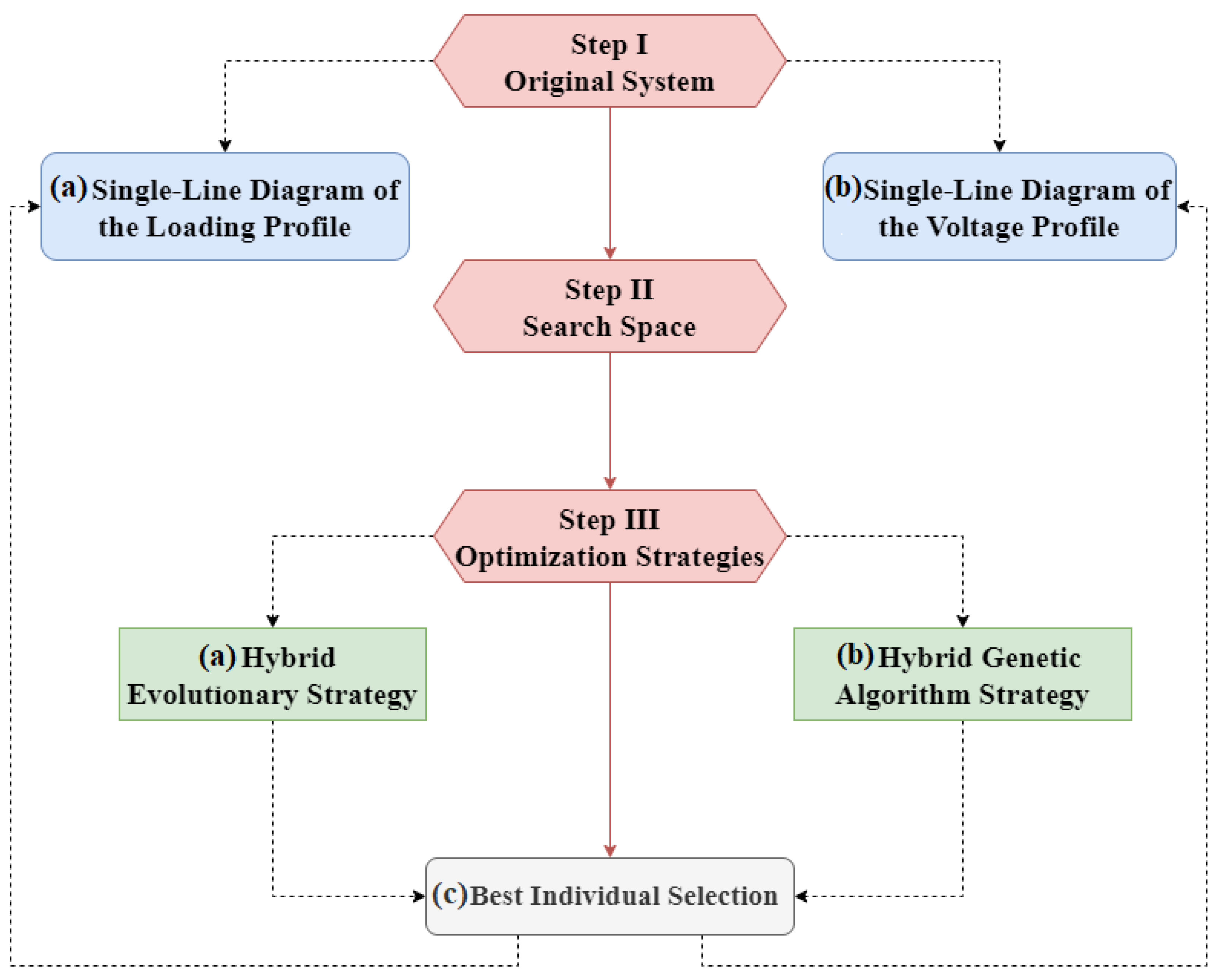
The computational tools used for system modeling and simulation were OpenDSS and QGIS. OpenDSS is an open-source software widely used for simulating EPDS, while QGIS is an open-source platform for Geographic Information Systems (GIS). This study employs a methodology divided into three main stages, illustrated in Figure 1. Each stage is designed to address different aspects of optimizing electric distribution systems, utilizing evolutionary and genetic strategies.

3.5. Stage I: Original System

In Stage I, the target Electric Distribution System and its main limitations are defined. A comprehensive survey of the characteristics and parameters of the original system is conducted, including topology, loads, and existing generation capacity. The system’s performance is evaluated without the allocation of Distributed Generation (DG) through simulations in the OpenDSS software. The input parameters for this evaluation include the following:

• Loads: Detailed information on the energy demands of the loads present in the system.
• Lines: Specific data on the distribution lines that make up the system.
• Available buses: Locations where DG resources can be allocated, which are characterized by the following:

  -

  Available area: Available space in the bus, considering environmental and spatial constraints, as discussed in Section 3.7.

  -

  Available Budget: Available budget for the construction of the power plant at the specified bus, also detailed in Section 3.7.

• Geographic Coordinates: Precise locations of load and line elements for an accurate geographical representation of the system.

The simulations in OpenDSS allow obtaining essential performance parameters, such as Bus Voltage Profile ($V_{\mathrm{i}}$), Active Power Losses in the Line ($P_{\mathrm{loss}}^{line,i}$), and Line Loading Profile ($C^{\mathrm{line},\mathrm{i}}$). Based on these parameters, important indicators for the Original System are defined:

• Total Losses ($P_{\mathrm{loss}}^{base}$): Sum of the losses in each line, as given by Equation (9), where i corresponds to the specific line and n to the number of the total lines in the system.

  $$P_{\mathrm{loss}}^{base}=\sum _{i=1}^n{P}_{\mathrm{loss}}^{line,i}$$

  (9)
• Violation of the upper voltage limit ($V_{\max }$): Counts the occurrences where the voltage profile at a bus exceeds the upper limit (in this case, set to 105%).
• Violation of the lower voltage limit ($V_{\min }$): Sums the occurrences where the voltage at a bus falls below the lower limit (in this case set to 95%)

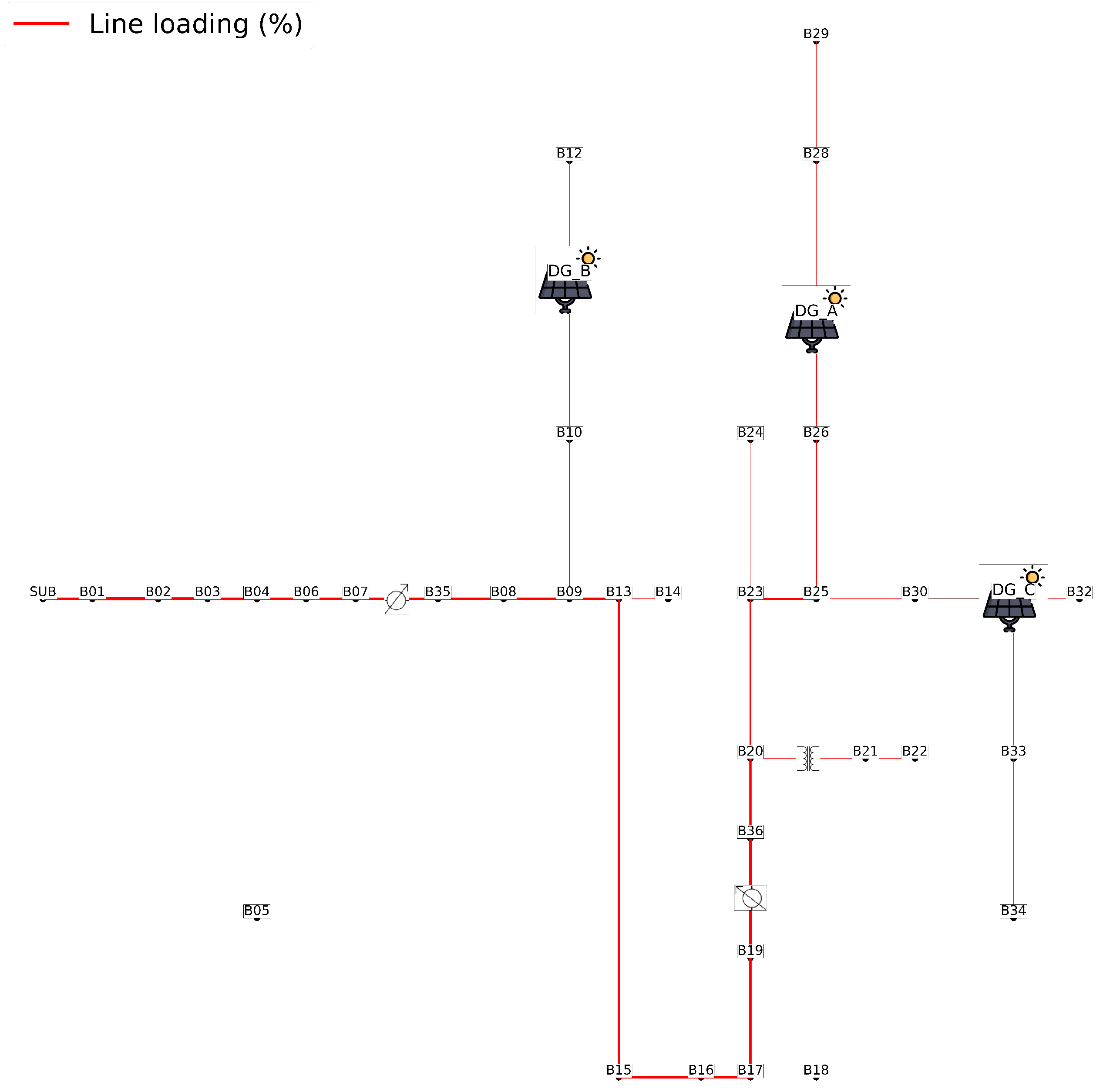
Both indicators, $V_{\max }$ and $V_{\min }$, are calculated for all buses in the system. Each violation is added to the corresponding total. After obtaining the performance indicators, the information from $V_{\mathrm{i}}$ and $C{L}_{\mathrm{i}}$ is used to plot the single-line diagrams of the loading profile and voltage profile behavior.

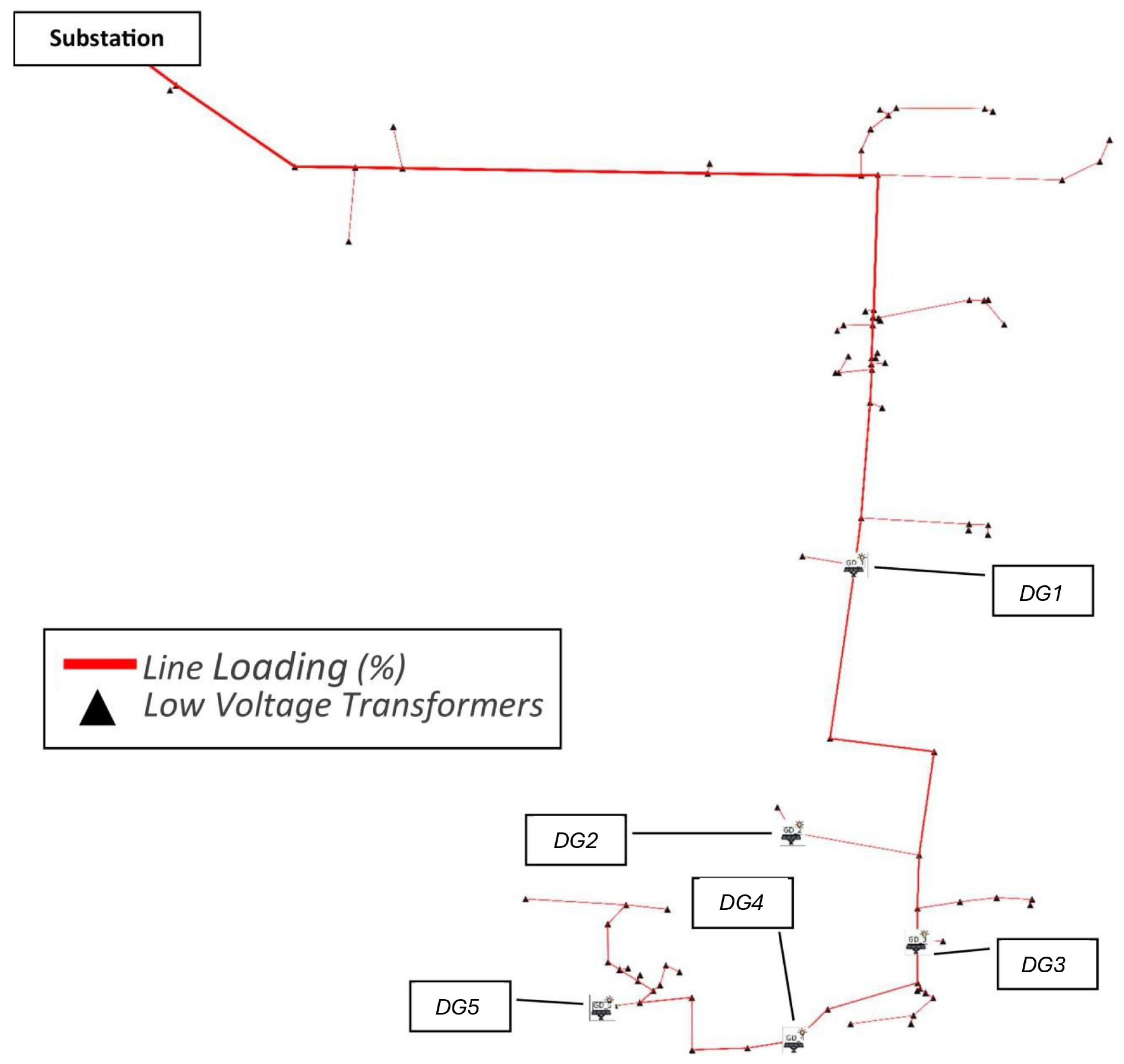
• Single-Line Diagram of the Loading Profile: The line thickness corresponds to the percentage of bus loading relative to the total system loading, obtained by summing the individual loadings.
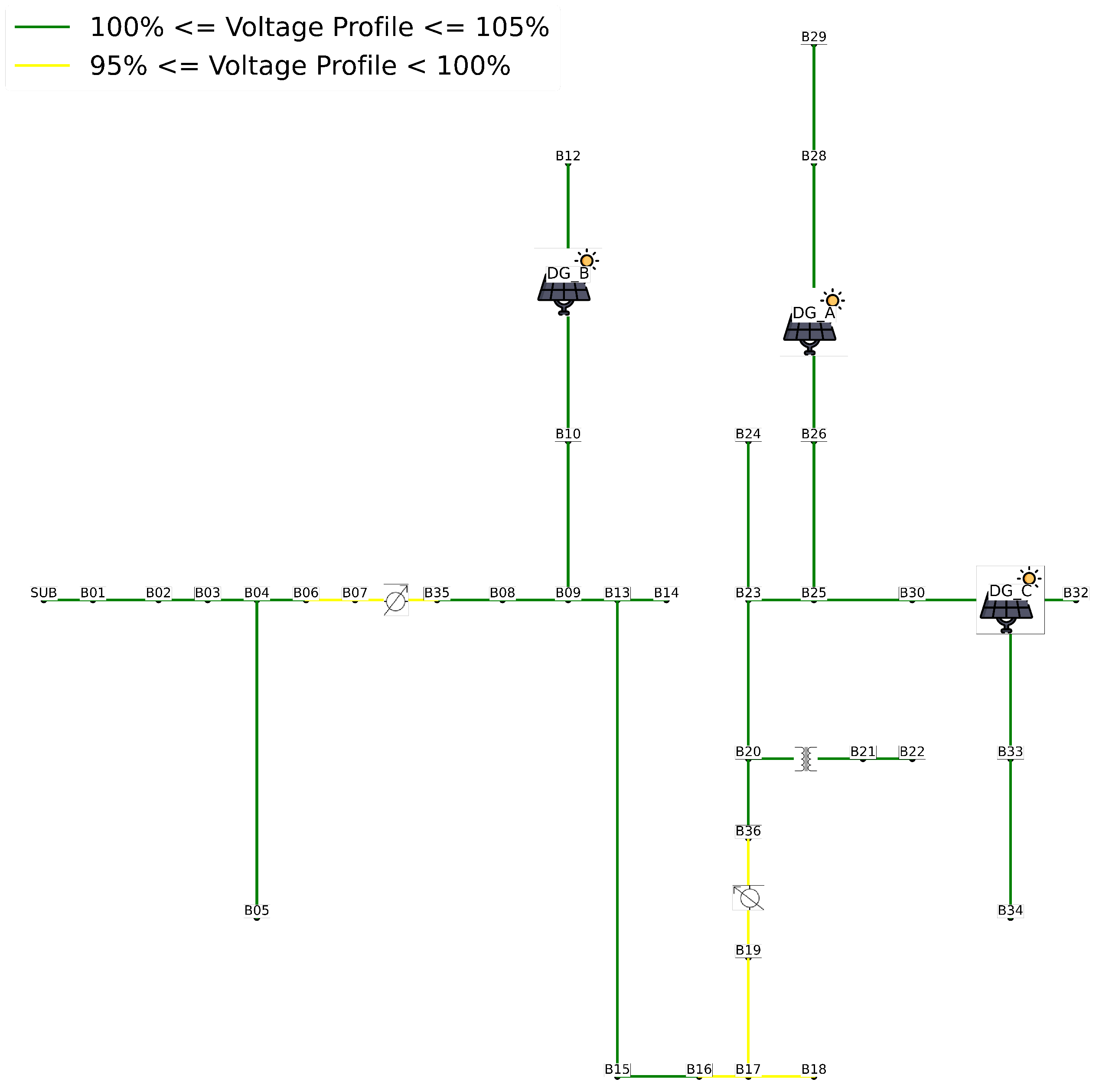
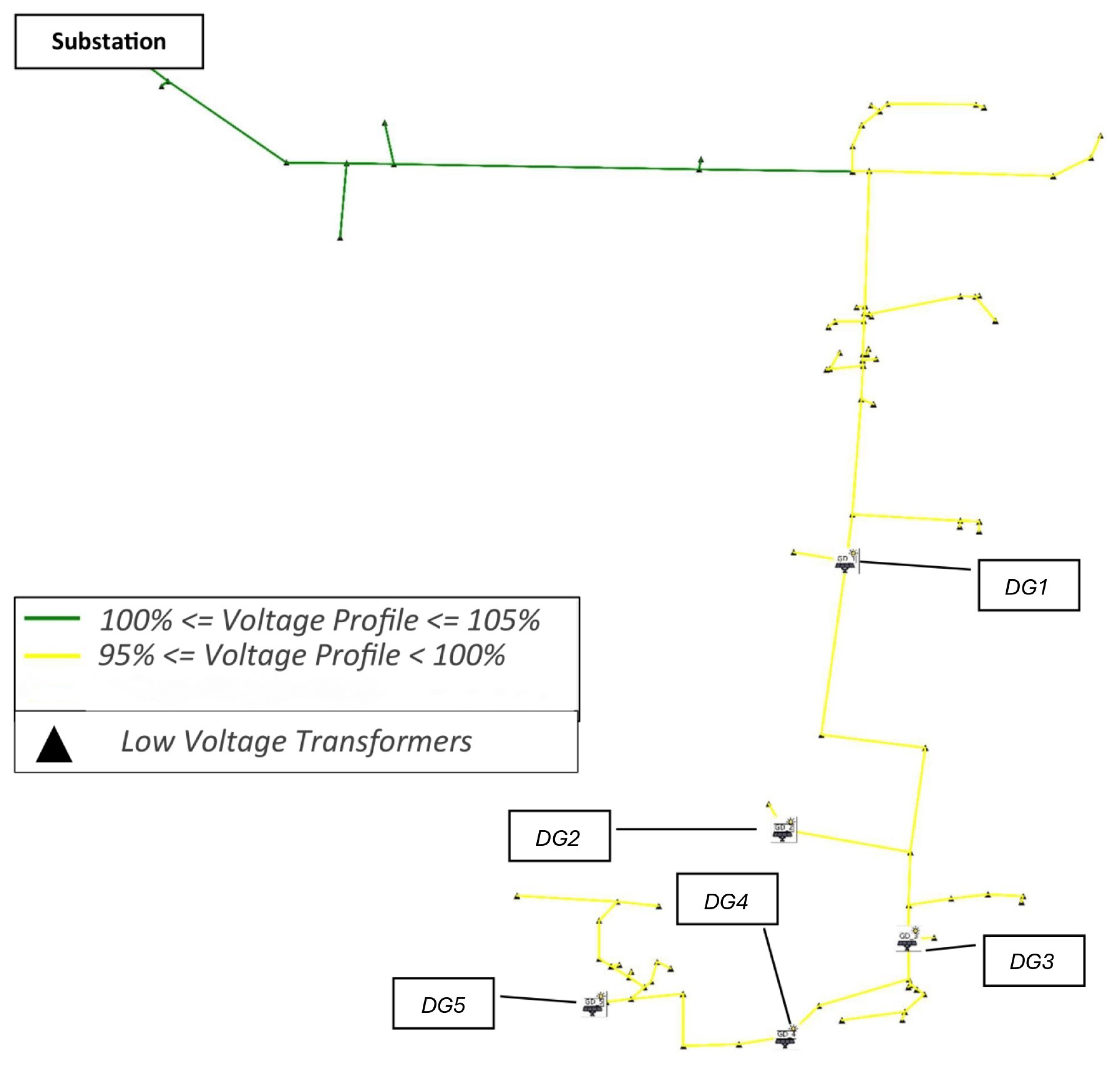
• Single-Line Diagram of the Voltage Profile: The voltage values per bus ($V_{\mathrm{i}}$) are interpreted in pu and plotted with colors according to the following criteria:

  -

  $V_{\mathrm{i}}>105\%$: Red.

  -

  $100\%\le V_{\mathrm{i}}\le 105\%$: Green.

  -

  $95\%\le V_{\mathrm{i}}<100\%$: Yellow.

  -

  $V_{\mathrm{i}}<95\%$: Blue.

These diagrams provide a clear visualization of the system’s behavior, both for the scenario without DG allocation and for scenarios with allocation throughout the EPDS.

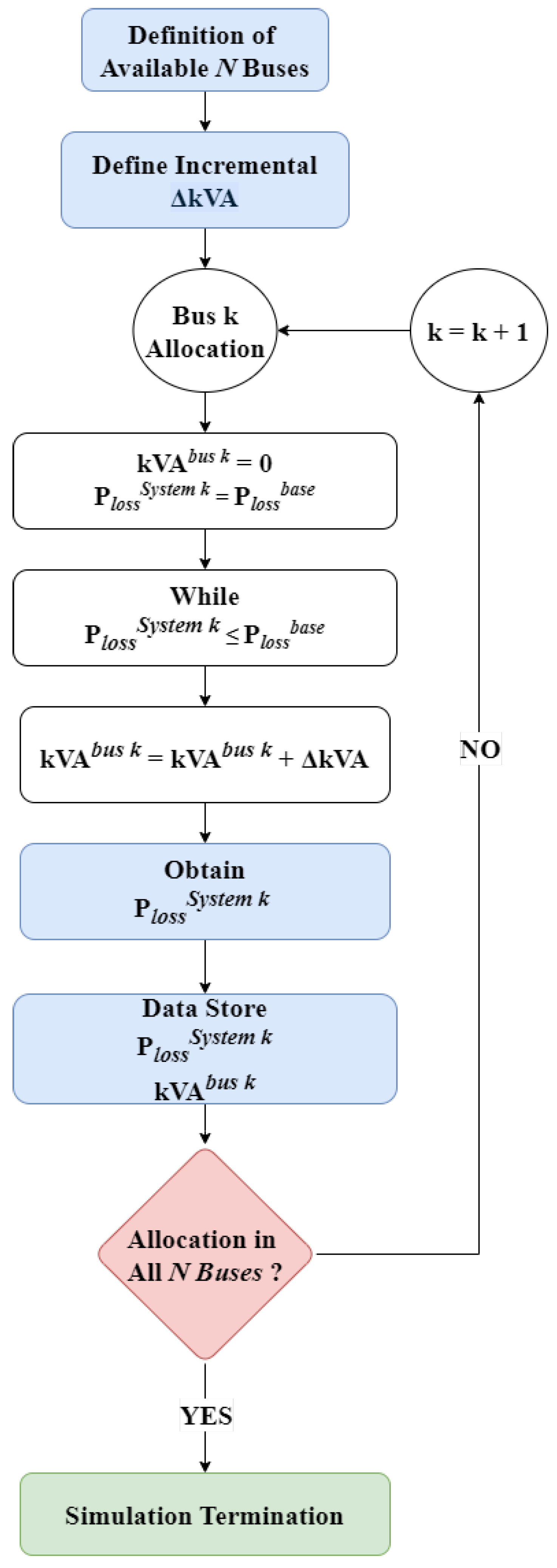
3.6. Stage II: Definition of the Search Space

This stage is initiated after defining the Distribution System and obtaining the performance indicators ($P_{\mathrm{loss}}^{base}$, $V_{\max }$, and $V_{\min }$) discussed in Section 3.5. Its objective is to determine the reference generation values for each bus, aiming to achieve the greatest reduction in total system losses by allocating a solar power plant to a specific bus. The procedure followed in this step is illustrated in the flowchart presented in Figure 2.

Using the available buses for DG allocation and defining the incremental power value $\Delta \mathrm{kVA}$, the procedure is as follows:

• Initialization: For each bus k, the following is defined:

  $$\left\{\begin{array}{c}\Delta {\mathrm{kVA}}^{\mathrm{bus}k}=0,\hfill \\ P_{\mathrm{loss}}^{\mathrm{System}k}=P_{\mathrm{loss}}^{base}\hfill \end{array}\right.$$

  (10)

  where $\Delta {\mathrm{kVA}}^{\mathrm{bus}k}$ is the generation power at bus k, and $P_{\mathrm{loss}}^{\mathrm{System}k}$ represents the system losses associated with that bus.
• Power Increment: As long as $P_{\mathrm{loss}}^{\mathrm{System}k}\le P_{\mathrm{loss}}^{base}$, the generation power at bus k is incremented by the following:

  $${\mathrm{kVA}}^{\mathrm{bus}k}\leftarrow {\mathrm{kVA}}^{\mathrm{bus}k}+\Delta {\mathrm{kVA}}^{\mathrm{bus}k},$$

  (11)

  where $\Delta {\mathrm{kVA}}^{\mathrm{bus}k}$ is the incremental power value defined for the study.
• Interruption: The increment process is stopped when $P_{\mathrm{loss}}^{\mathrm{System}k}>P_{\mathrm{loss}}^{base}$.

For each bus, the ideal power value that minimizes system losses is identified. This value corresponds to the minimum point of a parabolic curve associated with each bus. The resulting ideal power serves as a reference for the subsequent steps.

3.7. Stage III: Optimization Strategies

In this stage, a Hybrid Evolutionary Strategy and a Hybrid Genetic Algorithm are applied. Before discussing these algorithms, it is necessary to define the structure of the individuals, the selection, mutation, and crossover processes, and the evaluation of individual fitness.

3.7.1. Definition of Individuals

Each individual is represented by a vector of length l, where l is the total number of buses in the system. Each position in the vector takes a Boolean value (0 or 1) according to the following rule:

• Bus with DG allocated: Value 1.
• Bus without DG allocated: Value 0.

3.7.2. Initial Generation

Generation zero is created by defining a fixed number of individuals ($n_{\mathrm{individuals}}$) and the total number of generations ($n_{\mathrm{generations}}$). Additionally, the minimum ($\mathrm{minDGs}$) and maximum ($\mathrm{maxDGs}$) limits are established for the number of DG units allocated per individual. Each individual is generated randomly, while respecting the condition given by Equation (12). Individuals that do not meet these criteria or allocate DG units to unavailable buses are discarded.

$${\min }_{\mathrm{DGs}}\le {\mathrm{n}}_{\mathit{selected}\mathit{DGs}}\le {\max }_{\mathrm{DGs}}$$

(12)

3.7.3. Generation Capacity

For each allocated plant, the power, cost, and occupied area are calculated based on spatial and budgetary limitations. The following reference parameters are used.

$$\begin{array}{cc}\hfill {\mathrm{Cost}}_{\mathrm{Average}}& =4.02\mathrm{BRL}/\mathrm{kWp},\hfill \\ \hfill {\mathrm{Area}}_{\mathrm{Average}}& =10{\mathrm{m}}^2/\mathrm{kWp}\hfill \end{array}$$

(13)

The power plant capacity at bus k ($\mathrm{Power}{\mathrm{Plant}}_k$), its cost ($\mathrm{Plant}{\mathrm{Cost}}_k$), and occupied area ($\mathrm{Plant}{\mathrm{Area}}_k$) are defined as follows:

$$\begin{array}{cc}\hfill \mathrm{Power}{\mathrm{Plant}}_k& =\alpha ·\mathrm{Optimal}{\mathrm{Power}}_k,\hfill \\ \hfill \mathrm{Plant}{\mathrm{Cost}}_k& =\mathrm{Power}{\mathrm{Plant}}_k·{\mathrm{Cost}}_{\mathrm{Average}},\hfill \\ \hfill \mathrm{Plant}{\mathrm{Area}}_k& =\mathrm{Power}{\mathrm{Plant}}_k·{\mathrm{Area}}_{\mathrm{Average}},\hfill \end{array}$$

(14)

where $\alpha$ is a random value between 0 and 1. The value of $\alpha$ is adjusted until the following conditions are satisfied:

$$\begin{array}{cc}\hfill \mathrm{Plant}{\mathrm{Cost}}_k& \le {\mathrm{Budget}}_{\mathit{Constraint}\mathit{k}},\hfill \\ \hfill \mathrm{Plant}{\mathrm{Area}}_k& \le {\mathrm{Area}}_{\mathit{MaximumAvailable}k}\hfill \end{array}$$

(15)

3.7.4. Evaluation of Individual Fitness

After defining the individuals of generation zero and establishing their generation capacity, each individual is evaluated in terms of its fitness. During this evaluation, the following parameters are obtained:

• $P_{\mathrm{loss}}^j$: Total system losses with allocated DG units, calculated similarly to the original system ($P_{\mathrm{loss}}^{base}$).
• $V_{\mathit{max}}^j$: Number of buses with voltage above 105% (in pu) for the individual.
• $V_{\mathit{min}}^j$: Number of buses with voltage above 95% (in pu) for the individual.

The parameters $V_{\mathit{max}}^j$ and $V_{\mathit{min}}^j$ are evaluated between 6:00 a.m. and 6:00 p.m., the hours during which DG has the greatest influence on the system.

Although the intermittency of PV generation is not modeled through stochastic or probabilistic approaches, the temporal variability of solar irradiation is inherently considered through the use of a realistic solar radiation curve based on data generated by PVsyst. This curve is used in the OpenDSS simulations to model the time-varying behavior of PV generation throughout the day.

In this study, the DG units are therefore modeled as time-dependent energy sources, following the irradiance curve rather than assuming constant power injection. However, dispatching actions, curtailments, or disconnections of PV plants are not considered in the simulations. The objective is to evaluate the impact of distributed solar generation under normal operation scenarios, assuming full availability in accordance with the reference irradiance profile.

3.7.5. Selection Criteria

All individuals are subjected to the following selection criteria:

• Criterion 1: The voltage violations of the individual must not exceed those of the original system:

  $$V_{\mathit{max}}^j\le V_{\mathit{max}},$$

  (16)

  $$V_{\mathit{min}}^j\le V_{\mathit{min}}.$$

  (17)
• Criterion 2: The losses of the individual must be less than or equal to the average losses of the previous generation:

  $$P_{\mathrm{loss}}^j\le \mathrm{Average}{\mathrm{Loss}}_{\mathrm{Previous}\mathrm{Generation}}.$$

  (18)

Individuals that do not meet these criteria are discarded, ensuring that only feasible and efficient solutions are passed on to the next generations.

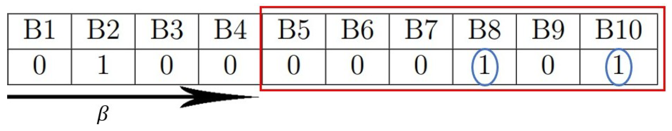
3.7.6. Mutation of Individuals

After selecting the fittest individual, the mutation process begins. It is considered a system with 10 buses, where a given individual has 2 DG units allocated and has the following constraints:

$$\begin{array}{c}\hfill {\min }_{\mathrm{DGs}}=2,\\ \hfill {\max }_{\mathrm{DGs}}=3.\end{array}$$

(19)

The mutation process consists of selecting segments to be preserved and applying a perturbation to the segments that will undergo mutation. The new mutated individual corresponds to the combination of the preserved segment with the perturbed segment. The key assumptions are as follows:

• Assumption 1: The size of the individual must not be altered. An individual with 10 buses before mutation will still have 10 buses after mutation.
• Assumption 2: The number of DG units allocated after mutation must respect the minimum and maximum limits defined in inequality (12).

To illustrate the process, suppose that $\beta =4$ is a random real parameter that defines up to which part of the individual will be preserved. For $\beta =4$, positions B1 to B4 are kept unchanged, while positions B5 to B10, highlighted by the red frame in Figure 3, are subject to mutation. In the preserved segment, there is one DG unit allocated; therefore, in the mutated segment, it is allowed to allocate between one and two DG units. After applying random Boolean values, a new mutated individual is obtained, as illustrated in Figure 3.

If the new individual does not satisfy Assumptions 1 and 2, it is discarded, and a new value of $\beta$ is drawn to perform a new mutation.

3.7.7. Crossover of Individuals

The crossover process consists of combining two parent individuals, which are randomly selected after the mutation stage. Each parent represents a distinct DG allocation configuration across 10 buses, as shown in

Table 2. Example of crossover between two individuals.

G	I	B1	B2	B3	B4	B5	B6	B7	B8	B9	B10
1	1	0	1	0	0	0	0	0	0	1	0
1	2	1	0	0	0	0	1	0	0	0	0

. This procedure enables the generation of new individuals by inheriting characteristics from both parents, thereby enhancing population diversity and improving the exploration of the search space.

The crossover process is defined by the parameters $\eta$ and $\delta$, which select specific segments from each “parent”. For $\eta =4$ and $\delta =6$, the selected segments are shown in Figure 4. The value of $\delta$ is calculated as follows:

$$\delta =l-\eta ,$$

(20)

where l is the total number of buses in the system.

The arrows in Figure 4 illustrate the segments selected for the crossover: the horizontal arrow labeled $\eta$ marks the portion taken from the first parent, while the arrow labeled $\delta$ indicates the segment taken from the second parent.

Once the segments have been defined, a third individual—referred to as the “Child”—is generated by combining selected portions from both “Parents”. This recombination process allows the child to inherit characteristics from each parent, promoting genetic diversity in the population. The resulting “Child”, along with the original “Parents”, is presented in

Table 3. Offspring resulting from the crossing of two distinct individuals (Parents).

G	I	B1	B2	B3	B4	B5	B6	B7	B8	B9	B10
1	1	0	1	0	0	0	0	0	0	1	0
1	2	1	0	0	0	0	1	0	0	0	0
1	F	0	1	0	0	0	1	0	0	0	0

.

The same assumptions previously defined for the mutation process also apply to the crossover operation. In addition, the two selected “Parents” must be distinct to ensure sufficient genetic diversity in the resulting “Child”. This diversity is essential for promoting variation within the population and enhancing the search for optimal solutions. The newly generated child will be included in the next generation of individuals.

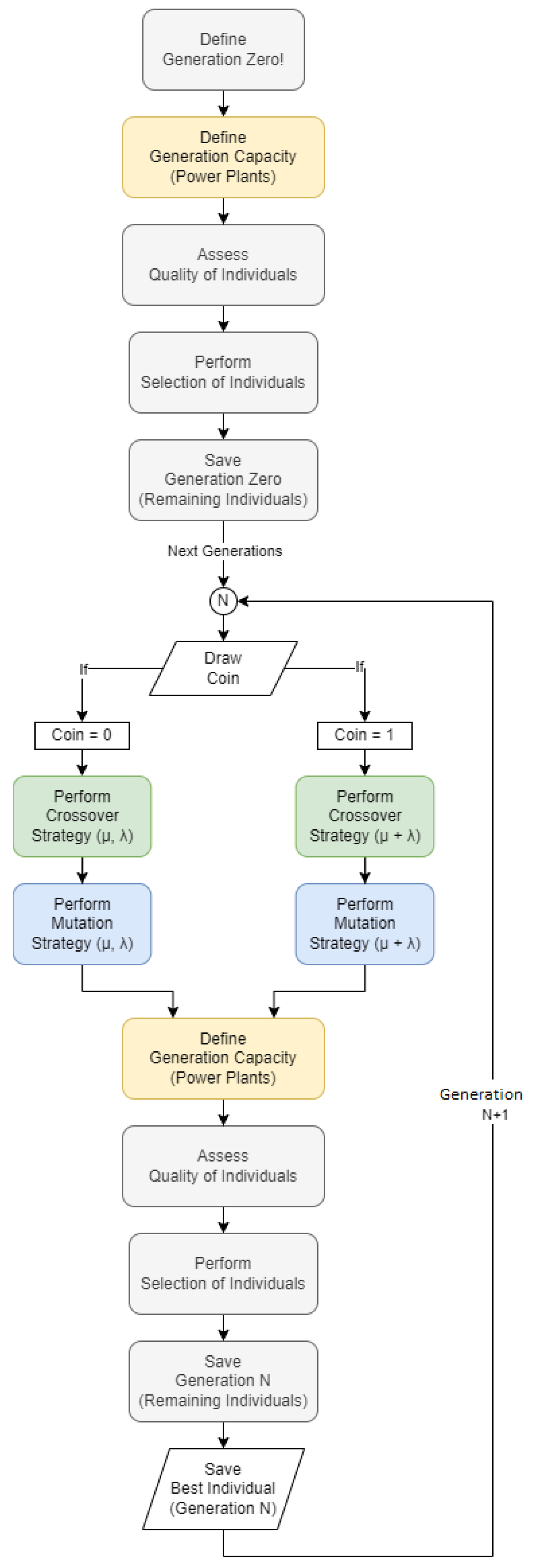
3.7.8. Hybrid Evolutionary Strategy

In this study, two variants of Evolutionary Strategies are employed: the $(\mu ,\lambda )$ and the $(\mu +\lambda )$. The Hybrid Evolutionary Strategy combines the benefits of both strategies throughout the generations, as illustrated in the flowchart in Figure 5.

The process begins with the definition of Generation Zero and the determination of each plant’s generation capacity. Next, the Selection of Individuals is performed, where the fittest individuals are chosen, and the remaining ones are stored for later reference. The decision between the $(\mu ,\lambda )$ and $(\mu +\lambda )$ strategies is made through a random draw (“Flip Coin”), where Coin = 0 applies the $(\mu ,\lambda )$ Evolutionary Strategy, and Coin = 1 applies the $(\mu +\lambda )$ Evolutionary Strategy.

Each new individual is created from an individual randomly selected among the $\mu$. Of the $\lambda$ individuals in the current generation, $\mu$ are retained in the $(\mu +\lambda )$ strategy, and the remaining $\lambda -\mu$ are generated by applying mutation to the selected $\mu$ individuals, thus maintaining a population of $\lambda$ individuals.

After selecting the $\mu$ fittest individuals in the $(\mu ,\lambda )$ strategy, all $\lambda$ individuals of the next generation are generated by applying mutation to the remaining $\mu$ individuals. Each new individual is created from a randomly selected individual among the $\mu$.

Out of the $\lambda$ individuals in the current generation, $\mu$ are retained in the $(\mu +\lambda )$ strategy, and the remaining $\lambda -\mu$ individuals are generated by applying mutation to the selected $\mu$ individuals, keeping the population size at $\lambda$ individuals.

After mutation, the individuals are evaluated based on their quality, and a new selection is performed. The best individual of each generation is the one with the lowest $P{T}_{\mathrm{j}}$ value, provided that $V{T}_{\max \mathrm{j}}$ and $V{T}_{\min \mathrm{j}}$ do not violate the limits of the Original System. At the end of all generations, the Overall Best Individual is selected from the best individuals of each generation.

3.7.9. Hybrid Genetic Algorithm Strategy

The main difference between the Hybrid GA Strategy and the Hybrid Evolutionary Strategy is the inclusion of crossover between two distinct individuals before the mutation process. The detailed flowchart is presented in Figure 6.

According to the flowchart, crossover occurs between individuals before the mutation process. The decision-maker “Flip Coin” is used to choose between Elitism $(\mu ,\lambda )$ (Coin = 0) and Elitism $(\mu +\lambda )$ (Coin = 1).

In the GA Strategy with Elitism $(\mu ,\lambda )$, crossover is performed between two distinct individuals among the fittest selected ones, generating a new individual. The number of new individuals is equal to the population size ($\lambda$), resulting in $\lambda$ offspring from crossover. These individuals then undergo the mutation process, generating $\lambda$ mutated individuals, which form the next generation.

In the GA Strategy with Elitism $(\mu +\lambda )$, the $\mu$ fittest individuals from the previous generation are retained. Additionally, two distinct individuals among the $\mu$ are selected to generate $\lambda -\mu$ new individuals through crossover. These new individuals then undergo mutation, resulting in $\lambda -\mu$ mutated individuals, which are combined with the $\mu$ retained individuals, forming a total of $\lambda$ individuals in the next generation.

After defining the $\lambda$ individuals of the new generation, the process continues with the determination of the generation capacity of the allocated plants, the evaluation of individual quality, and the selection of the best individuals. The remaining individuals are stored, and the process advances to the next generation.

3.7.10. Definition of the Best Individual

After applying the optimization strategies, the next step is to define the best individual for each strategy to identify the solution with the best performance in the Distribution System. This process is essential to validate the effectiveness of the methods used. The best individual is selected based on the following criteria:

• Performance Evaluation: Each individual is evaluated based on Total Losses ($P{T}_{\mathrm{Base}}$), Upper Voltage Violations ($V{T}_{\max }$), and Lower Voltage Violations ($V{T}_{\min }$). These parameters are analyzed for all system buses.
• Metric Comparison: Individuals are primarily compared based on the reduction of total losses. Additionally, it is verified whether the bus voltages remain within acceptable limits (95% to 105% in p.u).
• Final Selection: The best individual is the one that achieves the greatest reduction in total losses without voltage violations, ensuring system stability and efficiency.

This process ensures a rigorous and objective evaluation, allowing the identification of the most effective solution for the Distribution System. The analysis of the best individuals from each strategy provides valuable insights for future implementations.

4. Tests and Results

This section presents the results of applying the proposed methodology to two distinct case studies. The first case study employs the IEEE 34-bus system, a widely used benchmark feeder for power distribution system studies. The second case study is based on real-world data from the PD04 feeder of Neoenergia Brasilia, allowing the incorporation of spatial constraints and the analysis of the impact of DG allocation in a real scenario.

In both case studies, the Hybrid Evolutionary Strategy and the Hybrid Genetic Algorithm were assessed, with the aim of reducing overall system losses and enhance the voltage profile. The results are presented using tables and figures, which support the comparison of the performance of each strategy and allow for evaluating the impact of DG allocation on key system performance indicators.

4.1. Test Systems

Figure 7 illustrates the single-line diagram of the IEEE-34 bus test system, which comprises a total line length of 94 km, with five different configurations, including single-phase and three-phase lines; a supply voltage of 24.9 kV, with a section operating at 4.16 kV; nineteen distributed loads, totaling 2063.45 kVA; and two voltage regulators, each consisting of three single-phase transformers in a wye–wye configuration.

The second system, illustrated in Figure 8, is a medium-voltage feeder from Neoenergia Brasilia, operates at 13.8 kV, and has a total length of 40 km, with a total load of 4981 kVA. The system’s geographic modeling was carried out using QGIS software (Version 3.28.10) [35], and the data were obtained from the Distributor’s Geographic Database (BDGD). Low-Voltage (LV) loads were considered to be concentrated at their corresponding Medium-Voltage transformers.

The labels A1, A2, etc. in Figure 8, represent Area 1, Area 2, Area 3, and so on—indicating the potential areas available for the construction and placement of photovoltaic plants. The colors are merely visual aids used to distinguish and identify each area on the map.

Both systems were modeled and simulated in OpenDSS. Considering a 30% increase in both load and system extension, the resulting voltage profile shows that some bus voltages fall below the minimum limit of 95%. Additionally, total losses increase significantly. For the real system of Neoenergia Brasilia, the utility company allocated 18 areas for photovoltaic plants, with a budget of BRL 7.2 million, to mitigate voltage and loss issues. The location of these areas is shown in Figure 8.

4.2. Results with the IEEE 34-Bus System

For the IEEE 34-bus test system, a 30% increase in its installed capacity was assumed, which raised it from 2063.45 kVA to 2682.48 kVA. This increase led to a significant rise in total losses, which increased 133.40% (from 5958 kWh to 13,906 kWh.) Additionally, the system’s loading increased by 30.91% compared to the initial configuration. The resulting voltage profile is shown in Figure 9. The labels B01, B02, …, B34 in Figure 9 refer to the identification numbers of the buses in the IEEE 34-Bus distribution system. These labels are used to track the voltage magnitude at each bus along the feeder.

Figure 9 shows that, despite the implementation of two voltage regulators, it was not possible to keep the voltages of all buses above the minimum limit of 95%, as established in Section 2.2.1. The system loading after growth is illustrated in Figure 10.

To apply the proposed methodology, the construction of three photovoltaic plants was authorized, with a total installed generation capacity equivalent to 30% of the system’s current total installed power, given future demand growth. The new installed capacity of the plants is calculated using Equation (21).

$$\mathrm{Installed}{\mathrm{Capacity}}_{\mathrm{Plants}}=0.30\times \mathrm{Installed}{\mathrm{Capacity}}_{\mathrm{System}}=804.744\mathrm{kVA}$$

(21)

With the increment of load in both systems, some bus voltage magnitudes fall below the minimum limit of 95%. Additionally, total losses increase significantly. The proposed methodology aims to allocate and size photovoltaic plants to mitigate these issues and improve the performance of the distribution system.

4.2.1. Search Space Definition

For the application of the methodology, three photovoltaic plants were considered, with a total installed capacity of 804.744 kVA, corresponding to 30% of the system’s total power. This consideration aims to accommodate future demand growth while maintaining system stability. The optimal generation values for each bus, aimed at minimizing total system losses, were identified. All buses are available for the allocation of the plants.

Table 4. Lines with the best performance for single PV plant allocation per bus (IEEE 34-bus system).

Bus	Ideal PV Capacity (kW)	Reduction (%)
B23	231.79	4.28
B21	261.56	3.37
B09	270.47	2.91
B10	268.71	2.91

presents the four best alternatives for DG allocation along with their corresponding reduction in the system’s total power losses. Notably, when a DG is allocated at bus B23, a reduction of 4.23% is achieved. Also, when the DG is allocated at bus B21, a reduction of 3.37% is obtained, and so on. The optimal DG capacities for these locations range from 261.56 kW to 270.47 kW.

Table 5. Impacts of allocating DG at bus B23 (IEEE 34-bus system).

Voltage Increase (%)	Loss Reduction (%)	Loading Reduction (%)
5.43	4.28	2.36

highlights the benefits of integrating a 231.79 kW power plant at bus B23, which resulted in a 5.43% increase in the system’s average voltage, a 4.28% reduction in total losses, and a 2.36% decrease in loading.

4.2.2. Hybrid Evolutionary Strategy

The parameters used in the application of the Hybrid Evolutionary Strategy are as follows: Installed capacity of the plants: 804.744 kVA, minimum number of DGs: 2, and maximum number of DGs: 3.

Figure 11 illustrates the evolution of the best individual over the generations. The optimal solution was found in generation 55, which achieved a 14.42% reduction in total losses.

Table 6. Configuration of the three Plants—Hybrid Evolutionary Strategy (IEEE 34-bus system).

Bus	Installed Power (kW)	Phases	DG
B27	565.55	3	A
B11	178.83	1	B
B31	60.22	3	C

details the configuration of the three power plants that make up the system of the best individual. The total installed capacity was 804.60 kW.

The best individual resulted in a 7.09% voltage improvement, a 14.42% reduction in losses, and a 9.50% decrease in loading.

It is important to note that the Hybrid Evolutionary Strategy, by combining the $(\mu ,\lambda )$ and $(\mu +\lambda )$ approaches, achieves a balance between exploration and exploitation of the search space. This contributes to obtaining robust results, as evidenced by the significant reduction in losses and the improvement in the voltage profile. Additionally, the random selection of the strategy at each generation enhances the diversity of explored solutions, preventing premature convergence to local optima.

Comparing the results from Table 6 with those obtained in the Search Space Definition stage (Table 5), a substantial improvement can be observed across all metrics. The voltage improvement increases from 5.43% to 7.09%, the loss reduction jumps from 4.28% to 14.42%, and the loading reduction rises from 2.36% to 9.50%.

4.2.3. Hybrid Genetic Algorithm Strategy

The Hybrid Genetic Algorithm Strategy was applied to the system using the same constraints as the Hybrid Evolutionary Strategy. The optimal configuration of the three power plants is presented in

Table 7. Configuration of the 3 plants—Hybrid GA Strategy (IEEE 34-bus system).

Bus	Installed Power (kW)	Phases	DG
B11	615.61	3	A
B31	157.17	1	B
B23	31.82	1	C

, with a total installed capacity of 804.60 kW. The best individual achieved a 14.48% reduction in total losses, as shown in Figure 12.

The best individual achieved a voltage gain of 7.39%, a loss reduction of 14.48%, and a load reduction of 9.55%. Comparing the results from Table 7 with those obtained in the Search Space Definition stage (Table 5), a substantial improvement can be observed across all metrics. The voltage gain increases from 5.43% to 7.39%, the loss reduction jumps from 4.28% to 14.48%, and the load reduction rises from 2.36% to 9.55%.

It is interesting to note that the Hybrid GA Strategy shows a slight improvement over the Hybrid Evolutionary Strategy. This can be attributed to the inclusion of the crossover operator, which enhances the exploration of the search space by combining characteristics from different solutions, potentially discovering new and better system configurations. However, it is important to highlight that the Hybrid GA Strategy also has a higher computational cost due to the need to perform crossover between individuals.

4.2.4. Comparison of Strategies

The two optimization strategies (Hybrid Evolutionary Strategy and Hybrid GA Strategy) were compared with the Search Space Definition approach.

Table 8. Comparison of the performance of the best individuals (IEEE 34-bus system).

Strategy	Voltage Gain (%)	Loss Red. (%)	Loading Red. (%)
Search Space Def.	5.43	4.28	2.36
Hybrid ES	7.09	14.42	9.50
Hybrid GA	7.39	14.48	9.55

presents the results.

Both optimization strategies outperformed the Search Space Definition approach in all metrics, demonstrating the effectiveness of optimization in DG allocation. The Hybrid Genetic Algorithm (Hybrid GA) achieved the best performance, with voltage gains of 7.39%, loss reduction of 14.48%, and load reduction of 9.55%. This represents a significant improvement over the Hybrid Evolutionary Strategy, which obtained gains of 7.09%, 14.42%, and 9.50%, respectively. The Search Space Definition approach, on the other hand, showed the lowest gains, with 5.43%, 4.28%, and 2.36%.

The superiority of the Hybrid GA can be attributed to its ability to explore the search space more comprehensively by combining characteristics of different solutions through the crossover operator. This allows the algorithm to find potentially better solutions than those achieved by the Hybrid Evolutionary Strategy, which relies solely on mutation. However, the Hybrid GA also has a higher computational cost due to the need to perform crossover operations between individuals.

In summary, the choice of the optimization strategy depends on the specific requirements of the problem. If processing time is a critical factor, the Hybrid Evolutionary Strategy may be a more suitable option. On the other hand, if solution quality is the priority, the Hybrid GA may be the better choice despite its higher computational cost.

It is important to highlight that, in this case study, the Hybrid GA proved to be the best strategy for DG allocation in the IEEE 34-bus system. The results obtained demonstrate that incorporating the crossover operator can lead to higher-performing solutions compared to the Hybrid Evolutionary Strategy. However, the choice of strategy should be made considering the trade-off between solution quality and computational cost.

Figure 13 illustrates, through different colors, the voltage profile of the IEEE 34-bus test system after the optimal allocation of DG units. It is worth noting that all voltage levels are now above 95%. Furthermore, the loading profile is presented in Figure 14.

4.3. Results with the Real Feeder-PD04

With a projected 30% increase in load and system extension, the real feeder from Neoenergia Brasília will have a total installed capacity of 6475 kVA and an extension of 52 km. It is assumed that the extension increase occurs on the low-voltage side of the transformers, keeping the medium-voltage single-line diagram unchanged. The system’s voltage profile, considering this growth, is presented in Figure 15. It is observed that several buses exhibit voltages below the minimum limit of 95%. Additionally, the system will experience total losses of 6356 kWh, representing an increase of 2.91 times compared to the original system, along with an approximately 40% rise in total loading.

To mitigate these issues, the utility company decided to invest in the construction of photovoltaic plants, allocating 18 areas and a total budget of BRL 7.2 million. Figure 8 illustrates the location of these areas.

4.3.1. Search Space Definition

The “Search Space Definition” methodology (Section 3.6) was applied to identify the optimal generation values in each available area, with the aim of minimizing the system’s total losses. The 18 areas provided by the utility were individually evaluated, given the allocation of a power plant in each area.

Table 9. Areas with best performance for Individual Plant Allocation.

Bus	Area	Cost (MBRL)	Red. (%)	Power (kW)
B40	A9	4.93	9.99	1220.10
B60	A13	3.25	9.97	803.27
B28	A8	5.24	9.94	1296.44

presents the three areas with the highest loss reduction capacity, along with their estimated costs and maximum generation capacity.

Area A9 (Bus B40) shows the highest loss reduction (9.99%), with an installed capacity of 1220.10 kW and a cost of BRL 4.93 million. Areas A13 and A8 also stand out, with loss reductions of 9.97% and 9.94%, respectively.

4.3.2. Optimization of the Adopted Scenarios

Figure 16 presents the percentage reduction in the system’s total losses over 50 generations for three scenarios: 2DG, 3DG, and 5DG. The Hybrid GA Strategy was used to optimize the allocation of DGs, combining exploration and exploitation of solutions for efficient convergence.

The results show that the 5DG scenario achieved the highest loss reduction (14.05% in generation 34), surpassing the best result from Table 9 (9.99%). This difference occurs because the allocation of multiple DGs enables a more strategic distribution and a more efficient use of the available areas. The Hybrid GA Strategy contributed to this result by combining elitism with mutation and crossover operators, ensuring a robust and efficient evolution.

In the scenario with five DGs allocated at buses 50, 55, 62, 73, and 78, the total generated power was 1764.44 kW, with a total cost of BRL 7.09 million and a total area of 17,644.38 square meters (

Table 10. Information on allocated plants.

Plant	Power (kW)	Area (m2)	Cost (MBRL)	Area
DG 1	12.76	127.59	0.05	A11
DG 2	420.37	4203.65	1.69	A12
DG 3	262.48	2624.78	1.05	A14
DG 4	398.35	3983.52	1.60	A18
DG 5	670.48	6704.84	2.70	A16
Total	1764.44	17,644.38	7.09	–

). The cost remained within the BRL 7.2 million budget, with 98.47% utilization. The calculated areas for each DG complied with spatial constraints.

The allocation of the five DGs resulted in a 1.75% improvement in the voltage profile, a 14.08% reduction in total system losses, and an 8.90% decrease in loading (

Table 11. System performance with five allocated DGs.

Voltage Gain (%)	Loss Reduction (%)	Load Reduction (%)
1.75	14.08	8.90

).

The significant reduction in total system losses validates the effectiveness of the DG allocation strategy. The resulting voltage and loading profiles are illustrated in Figure 17 and Figure 18, respectively. In summary, the allocation of five DGs proved to be both efficient and feasible, leading to improvements in system performance, particularly in loss reduction.

Beyond numerical improvements, the optimization process fostered robust distribution network configurations, which are better equipped to handle operational stress and variability in load and generation. By reducing overloading and voltage deviations, the system complies more consistently with technical quality standards, thus contributing to improved power supply quality and operational reliability. In addition, the implemented metaheuristic algorithms proved to be efficient in finding solutions within complex, nonlinear, and multi-constrained search spaces inherent to distributed generation (DG) planning problems. By balancing global exploration and local exploitation, these algorithms achieve high-quality solutions, prioritizing technical efficiency as a main objective in DG allocation and sizing.

5. Conclusions

This study proposed an innovative methodology for optimizing the allocation and sizing of photovoltaic distributed generation (DG) in electrical distribution systems. The main contribution lies in the integration of georeferenced spatial constraints into the optimization process, in addition to conventional technical and budgetary limitations. This multi-criteria approach enhances the realism of DG planning and ensures compatibility with physical and economic feasibility.

The methodology combines simulations in OpenDSS and QGIS with metaheuristic techniques, specifically the Hybrid Evolutionary Strategy and Hybrid Genetic Algorithm. Two case studies were conducted to validate the approach: the standard IEEE 34-bus distribution system and a real medium-voltage feeder. In both cases, the optimization model successfully identified the DG configurations that improved the performance of the system.

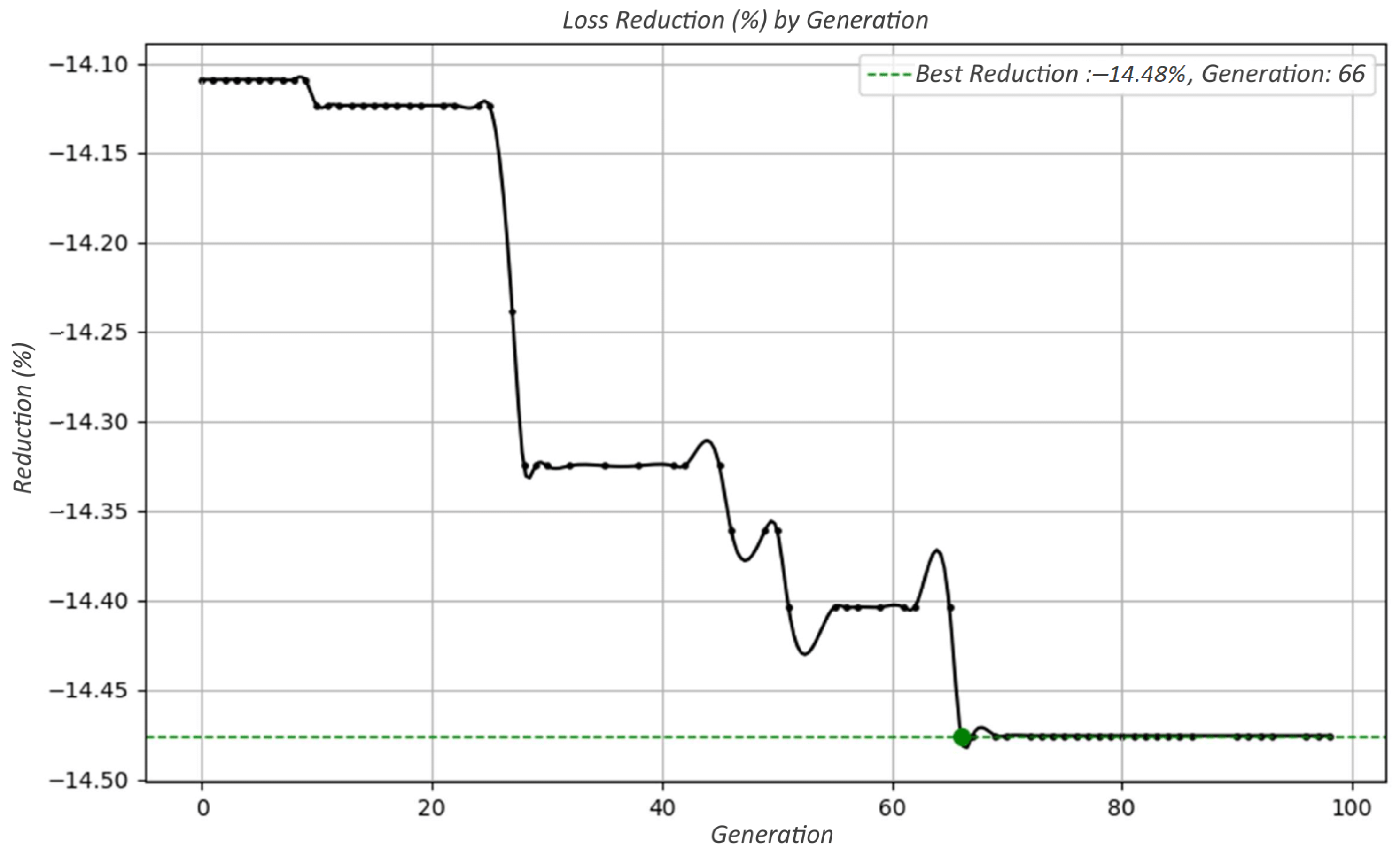
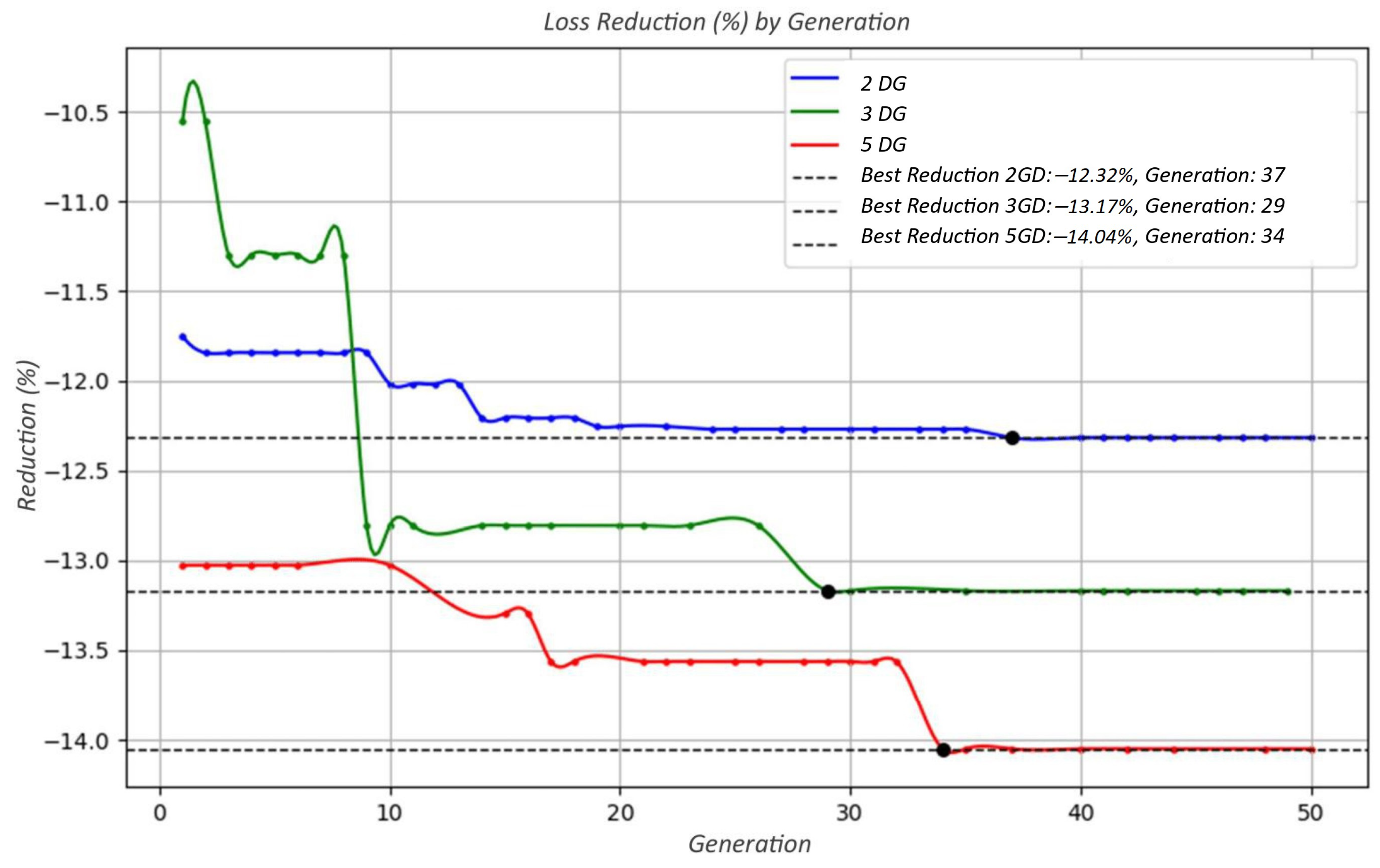
Quantitative results confirm the effectiveness of the methodology. In the IEEE 34-bus system, the allocation of photovoltaic units led to a 14.48% reduction in total energy losses and a 7.39% improvement in the voltage profile. For the real feeder, a similar strategy resulted in a loss reduction of 14.08% and an enhancement of 1.75% in voltage levels. These improvements demonstrate the technical value of properly allocated DG units, particularly when spatial feasibility is considered.

Furthermore, the use of hybrid metaheuristics provided robust convergence and high-quality solutions in a non-convex, multi-constrained optimization environment. The combination of spatial, technical, and economic constraints proved essential for producing feasible and efficient DG planning strategies.

References

1. International Renewable Energy Agency. Renewable Power Generation Costs in 2023. 2024. Available online: https://www.irena.org/Publications/2024/Sep/Renewable-Power-Generation-Costs-in-2023 (accessed on 1 March 2025).
2. Segreto, M.; Principe, L.; Desormeaux, A.; Torre, M.; Tomassetti, L.; Tratzi, P.; Paolini, V.; Petracchini, F. Trends in Social Acceptance of Renewable Energy Across Europe—A Literature Review. Int. J. Environ. Res. Public Health 2020, 17, 9161. [Google Scholar] [CrossRef] [PubMed]
3. Mehigan, L.; Deane, J.; Gallachóir, B.; Bertsch, V. A review of the role of distributed generation (DG) in future electricity systems. Energy 2018, 163, 822–836. [Google Scholar] [CrossRef]
4. López-Lezama, J.M.; Cortina-Gómez, J.; Muñoz-Galeano, N. Assessment of the Electric Grid Interdiction Problem using a nonlinear modeling approach. Electr. Power Syst. Res. 2017, 144, 243–254. [Google Scholar] [CrossRef]
5. Ahmed, A.; Hasan, S. Optimal allocation of distributed generation units for converting conventional radial distribution system to loop using particle swarm optimization. Energy Procedia 2018, 153, 118–124. [Google Scholar] [CrossRef]
6. Arif, S.M.; Hussain, A.; Lie, T.T.; Ahsan, S.M.; Khan, H.A. Analytical Hybrid Particle Swarm Optimization Algorithm for Optimal Siting and Sizing of Distributed Generation in Smart Grid. J. Mod. Power Syst. Clean Energy 2020, 8, 1221–1230. [Google Scholar] [CrossRef]
7. Farh, H.M.H.; Al-Shaalan, A.M.; Eltamaly, A.M.; Al-Shamma’A, A.A. A Novel Crow Search Algorithm Auto-Drive PSO for Optimal Allocation and Sizing of Renewable Distributed Generation. IEEE Access 2020, 8, 27807–27820. [Google Scholar] [CrossRef]
8. Farh, H.M.; Al-Shaalan, A.M.; Eltamaly, A.M.; Al-Shamma’a, A.A. A novel severity performance index for optimal allocation and sizing of photovoltaic distributed generations. Energy Rep. 2020, 6, 2180–2190. [Google Scholar] [CrossRef]
9. Farh, H.M.H.; Eltamaly, A.M.; Al-Shaalan, A.M.; Al-Shamma’a, A.A. A novel sizing inherits allocation strategy of renewable distributed generations using crow search combined with particle swarm optimization algorithm. IET Renew. Power Gener. 2021, 15, 1436–1450. [Google Scholar] [CrossRef]
10. de Carvalho, T.L.A.; Ferreira, N.R. Optimal allocation of distributed generation using ant colony optimization in electrical distribution system. In Proceedings of the 2018 Simposio Brasileiro de Sistemas Eletricos (SBSE), Niteroi, Brazil, 12–16 May 2018; pp. 1–6. [Google Scholar] [CrossRef]
11. Zakaria, Y.Y.; Swief, R.A.; El-Amary, N.H.; Ibrahim, A.M. Optimal Distributed Generation Allocation and Sizing Using Genetic and Ant Colony Algorithms. J. Phys. Conf. Ser. 2020, 1447, 012023. [Google Scholar] [CrossRef]
12. Ganguly, S.; Samajpati, D. Distributed Generation Allocation on Radial Distribution Networks Under Uncertainties of Load and Generation Using Genetic Algorithm. IEEE Trans. Sustain. Energy 2015, 6, 688–697. [Google Scholar] [CrossRef]
13. Purlu, M.; Turkay, B.E. Optimal Allocation of Renewable Distributed Generations Using Heuristic Methods to Minimize Annual Energy Losses and Voltage Deviation Index. IEEE Access 2022, 10, 21455–21474. [Google Scholar] [CrossRef]
14. Almabsout, E.A.; El-Sehiemy, R.A.; An, O.N.U.; Bayat, O. A Hybrid Local Search-Genetic Algorithm for Simultaneous Placement of DG Units and Shunt Capacitors in Radial Distribution Systems. IEEE Access 2020, 8, 54465–54481. [Google Scholar] [CrossRef]
15. Zuluaga-Ríos, C.D. A modified and extended genetic algorithm for optimal distributed generation grid-integration solutions in direct current power grids. e-Prime Adv. Electr. Eng. Electron. Energy 2024, 10, 100857. [Google Scholar] [CrossRef]
16. Sheng, W.; Liu, K.Y.; Liu, Y.; Meng, X.; Li, Y. Optimal Placement and Sizing of Distributed Generation via an Improved Nondominated Sorting Genetic Algorithm II. IEEE Trans. Power Deliv. 2015, 30, 569–578. [Google Scholar] [CrossRef]
17. Ganguly, S.; Samajpati, D. Distributed generation allocation with on-load tap changer on radial distribution networks using adaptive genetic algorithm. Appl. Soft Comput. 2017, 59, 45–67. [Google Scholar] [CrossRef]
18. Hamidi, M.E.; Chabanloo, R.M. Optimal Allocation of Distributed Generation With Optimal Sizing of Fault Current Limiter to Reduce the Impact on Distribution Networks Using NSGA-II. IEEE Syst. J. 2019, 13, 1714–1724. [Google Scholar] [CrossRef]
19. Nagaballi, S.; Kale, V.S. Pareto optimality and game theory approach for optimal deployment of DG in radial distribution system to improve techno-economic benefits. Appl. Soft Comput. 2020, 92, 106234. [Google Scholar] [CrossRef]
20. Kamel, S.; Khasanov, M.; Jurado, F.; Kurbanov, A.; Zawbaa, H.M.; Alathbah, M.A. Simultaneously Distributed Generation Allocation and Network Reconfiguration in Distribution Network Considering Different Loading Levels. IEEE Access 2023, 11, 105916–105934. [Google Scholar] [CrossRef]
21. Gao, F.; Yuan, C.; Li, Z.; Zhuang, S. Multi-objective optimal allocation of distributed generation considering the spatiotemporal correlation of wind-photovoltaic-load. Electr. Power Syst. Res. 2023, 214, 108914. [Google Scholar] [CrossRef]
22. Zhao, Q.; Wang, S.; Wang, K.; Huang, B. Multi-objective optimal allocation of distributed generations under uncertainty based on D-S evidence theory and affine arithmetic. Int. J. Electr. Power Energy Syst. 2019, 112, 70–82. [Google Scholar] [CrossRef]
23. Cao, Q.; Wang, H.; Hui, Z.; Chen, L. Optimal Location and Sizing of Multi-Resource Distributed Generator Based on Multi-Objective Artificial Bee Colony Algorithm. Energy Eng. 2024, 121, 499–521. [Google Scholar] [CrossRef]
24. Sharma, R.K.; Naick, B.K. A novel quasi oppositional artificial rabbits optimization algorithm for optimal distributed generation allocation in radial distribution systems under different load models. Comput. Electr. Eng. 2025, 122, 109965. [Google Scholar] [CrossRef]
25. Tolabi, H.; Ara, A.L.; Hosseini, R. A new thief and police algorithm and its application in simultaneous reconfiguration with optimal allocation of capacitor and distributed generation units. Energy 2020, 203, 117911. [Google Scholar] [CrossRef]
26. Nizamani, Q.; Hashmani, A.A.; Leghari, Z.H.; Memon, Z.A.; Munir, H.M.; Novak, T.; Jasinski, M. Nature-inspired swarm intelligence algorithms for optimal distributed generation allocation: A comprehensive review for minimizing power losses in distribution networks. Alex. Eng. J. 2024, 105, 692–723. [Google Scholar] [CrossRef]
27. Pesaran, H.A.M.; Huy, P.D.; Ramachandaramurthy, V.K. A review of the optimal allocation of distributed generation: Objectives, constraints, methods, and algorithms. Renew. Sustain. Energy Rev. 2017, 75, 293–312. [Google Scholar] [CrossRef]
28. Saad, O.; Abdeljebbar, C. Historical Literature Review of Optimal Placement of Electrical Devices in Power Systems: Critical Analysis of Renewable Distributed Generation Efforts. IEEE Syst. J. 2021, 15, 3820–3831. [Google Scholar] [CrossRef]
29. Guzmán-Henao, J.A.; Bolaños, R.I.; Montoya, O.D.; Grisales-Noreña, L.F.; Chamorro, H.R. On Integrating and Operating Distributed Energy Resources in Distribution Networks: A Review of Current Solution Methods, Challenges, and Opportunities. IEEE Access 2024, 12, 55111–55133. [Google Scholar] [CrossRef]
30. Megantoro, P.; Halim, S.A.; Kamari, N.A.M.; Awalin, L.J.; Ali, M.S.; Rosli, H.M. Optimizing reactive power dispatch with metaheuristic algorithms: A review of renewable distributed generation integration with intermittency considerations. Energy Rep. 2025, 13, 397–423. [Google Scholar] [CrossRef]
31. Nassar, S.M.; Saleh, A.; Eisa, A.A.; Abdallah, E.; Nassar, I.A. Optimal allocation of renewable energy resources in distribution systems using meta-heuristic algorithms. Results Eng. 2025, 25, 104276. [Google Scholar] [CrossRef]
32. Electric Power Research Institute (EPRI). OpenDSS—Electric Power Distribution System Simulator, Version 10.2.0.1—Columbus. Available online: https://www.epri.com/pages/sa/opendss (accessed on 15 April 2025).
33. Python Software Foundation. Python Language Reference, Version 3.10. Available online: https://www.python.org (accessed on 15 April 2025).
34. Luke, S. Essentials of Metaheuristics, 2nd ed.; Lulu: Morrisville, NC, USA, 2013; Available online: http://cs.gmu.edu/~sean/book/metaheuristics/ (accessed on 1 March 2025).
35. QGIS Development Team. QGIS Geographic Information System, Version 3.28.10. Open Source Geospatial Foundation Project. Available online: https://www.qgis.org (accessed on 15 April 2025).
Figure 1. Flowchart of the general methodology.
Energies 18 02091 g001
Figure 2. Search space flowchart.
Energies 18 02091 g002
Figure 3. Individual after applying mutation.
Energies 18 02091 g003
Figure 4. Individual after mutation.
Energies 18 02091 g004
Figure 5. Flowchart of the Hybrid Evolutionary Strategy.
Energies 18 02091 g005
Figure 6. Hybrid Elitism flowchart.
Energies 18 02091 g006
Figure 7. Single-line diagram of the IEEE 34-bus system.
Energies 18 02091 g007
Figure 8. Real System PD04–Areas provided by the utility company.
Energies 18 02091 g008
Figure 9. Voltage profile of the IEEE 34-Bus System after a 30% growth.
Energies 18 02091 g009
Figure 10. Loading profile of the IEEE 34-Bus System after a 30% growth.
Energies 18 02091 g010
Figure 11. Behavior of the Best Individual over Generations—Hybrid Evolutionary Strategy (IEEE 34-bus system).
Energies 18 02091 g011
Figure 12. Behavior of the Best Individual over Generations—Hybrid GA Strategy (IEEE 34-bus system).
Energies 18 02091 g012
Figure 13. Voltage profile—Hybrid Evolutionary Strategy (IEEE 34-bus system).
Energies 18 02091 g013
Figure 14. Loading profile—Hybrid Evolutionary Strategy (IEEE 34-bus system).
Energies 18 02091 g014
Figure 15. Voltage profile with 30% growth (Real System PD04).
Energies 18 02091 g015
Figure 16. Comparison of Scenario Performance over generations.
Energies 18 02091 g016
Figure 17. System Voltage Profile—5 Allocated DGs.
Energies 18 02091 g017
Figure 18. System Load Profile—5 Allocated DGs.
Energies 18 02091 g018