A Reactive Power Partitioning Method Considering Source–Load Correlation and Regional Coupling Degrees

Abstract

To address the enhanced coupling characteristics in reactive power partitioning of power grids with high-penetration renewable energy integration, this paper proposes an optimized reactive power partitioning method that integrates dynamic source–load correlation characteristics and regional coupling degree evaluation. Conventional static electrical distance-based partitioning methods struggle to adapt to dynamic coupling effects caused by renewable energy output fluctuations, leading to degraded partition decoupling performance. This study innovatively constructs a Copula function-based joint probability distribution model for source–load correlation. By employing non-parametric estimation and undetermined coefficient methods to solve marginal distribution parameters, and utilizing the K-means clustering algorithm to generate typical scenario sets, a comprehensive source–load coupling evaluation framework is established, incorporating the renewable energy output proportion and time-varying correlation index. For electrical distance calculation, a generalized construction method for extended sensitivity matrices is proposed, featuring dynamic weight adjustment through regional coupling degree correction factors. Simulation results demonstrate that in practical case studies, compared with traditional partitioning schemes, the proposed method reduces the regional coupling degree metric by 4.216% and enhances the regional reactive power imbalance index suppression by 11.082%, validating its effectiveness in achieving reactive power local balance and reactive power partitioning. This research breaks through the theoretical limitations of static partitioning and provides theoretical support for dynamic zonal control in modern power systems with high renewable penetration.

1. Introduction

The rapid integration of high-penetration renewable energy sources into modern power systems has introduced unprecedented challenges to grid stability and control. Traditional reactive power partitioning methods, which rely on static electrical distance metrics (e.g., nodal impedance matrices) [1,2,3,4], are designed for grids with predictable operational trends. However, the inherent volatility of renewable energy sources, such as wind and solar power, amplifies dynamic coupling effects between generation and demand, rendering conventional partitioning strategies ineffective. These static approaches often fail to adapt to time-varying source–load correlations and regional interdependencies, leading to suboptimal partitions, increased reactive power exchange, and voltage instability [5,6,7,8]. On the basis of the above, Xiao [9] proposed a spatiotemporal cooperative zoning control architecture that achieves network decoupling through community detection algorithms but failed to quantify the impact of source–load spatiotemporal correlations on zoning stability. Wu [10] designed a three-stage dynamic optimization strategy incorporating PAM clustering to constrain the action frequency of discrete devices, but their zoning coupling degree evaluation system remains incomplete. However, the overall modeling of spatiotemporal dependence while compensating for prediction uncertainty is a gap that is still not fully addressed in the existing literature. Unlike the aforementioned methods, this paper constructs a Copula-based joint probability model to not only quantify the impact of spatiotemporal source–load correlations on partition stability but also introduces dynamic correction factors and composite coupling metrics, addressing the incompleteness of existing partition coupling degree evaluation frameworks.

Recent advancements in probabilistic modeling have highlighted the potential of Copula-based methods for capturing complex dependencies in renewable generation. For instance, Krishna and Abhyankar [11] proposed a Regular Vine (R-vine) Copula framework combined with uniform design sampling to generate wind power scenarios with reduced variance, demonstrating significant improvements in temporal dependence modeling. Building on this, Ye et al. [12] extended Copula applications to multi-wind farm scenarios using kernel density estimation, though their method overlooked the propagation of forecast errors in downstream optimization. Meanwhile, Yoo et al. [13] introduced a binned empirical cumulative distribution function (ECDF) approach to compensate for forecast errors; yet, their spatial–temporal correlation analysis lacked granularity. While these studies underscore the versatility of Copulas in renewable energy sources modeling, critical gaps persist:

• Variance reduction techniques and forecast error compensation (e.g., error binning [13]) are rarely integrated into partitioning frameworks, leading to instability in dynamic grid operations.
• Existing indices focus narrowly on nodal electrical distances [14], ignoring temporal synchronization between renewable energy sources generation and load profiles, thereby undermining the reactive power balance within partitions.

To resolve these issues, the proposed method aims to bridge the theoretical and practical gaps through the innovations of proposing a composite coupling index that incorporates temporal synchronization between renewable generation and load profiles, thereby optimizing the local reactive power balance. The key innovations include the following:

• In Section 2.1, a Gaussian Copula-based joint probability model captures the stochastic dependence between renewable energy sources and load demand, followed by scenario reduction via K-means clustering to generate key representative scenarios.
• In Section 3, the electrical distance matrix integrated with correction factors can more effectively capture the variability of renewable energy sources, making it suitable for the current trend of increasing renewable energy sources penetration levels.
• A hierarchical clustering framework driven by a composite coupling index, ensuring partitions with minimized intra-regional electrical distances and maximized inter-regional decoupling.

Verified on the IEEE 39-bus system, compared to existing methods, this approach improves the regional coupling degree metric and reduces the regional reactive power imbalance. This work not only advances the theoretical foundation of dynamic partitioning but also provides actionable insights for optimizing reactive power dispatch in grids with high renewable energy sources penetration.

The remainder of this paper is organized as follows: Section 2 details the source–load correlation modeling; Section 3 introduces the modified electrical distance calculation; Section 4 presents the regional coupling degree metrics and describes the partitioning algorithm; Section 5 validates the method through case studies; and Section 6 concludes the work.

2. Calculation of the Dynamic Source–Load Correlation Index

2.1. Construct a Source–Load Correlation Model Based on Copula Function

In this paper, we need to periodically obtain the output data of all grid-connected new energy generation equipment and the consumer-side electric load data in the grid to be partitioned, and the above data are called source–load data. The source–load data are fitted to obtain the marginal distribution of the source–load data.

Construct a source–load correlation model based on the Copula function based on the marginal distribution of source–load data.

Based on the properties of the Copula function as mentioned in [6,15], let $F\left(x_1,x_2,\cdots x_M\right)$ be the joint probability distribution function with marginal distributions$F_1\left(x_1\right)$, $F_2\left(x_2\right)$, $\cdots F_M\left(x_M\right)$, respectively, then there must exist a Copula function $C\left[F_1\right(x_1),F_2(x_2),\cdots F_M(x_M\left)\right]$, which satisfies:

$$F\left(x_1,x_2,\cdots ,x_M\right)=C\left[F_1\left(x_1\right),F_2\left(x_2\right),\cdots ,F_M\left(x_M\right)\right]=C\left[u_1,u_2,\cdots u_M\right]$$

(1)

Derivation of (1) yields the corresponding joint probability density function:

$$f\left(x_1,x_2,\cdots x_M\right)=c\left(\mathit{u}\right){\prod }_{m=1}^{M}f\left(x_m\right)$$

(2)

where $c\left(\mathit{u}\right)$ is the probability density function of the Copula function; $u_m=F_m\left(x_m\right)$; $\mathit{u}=(u_1,u_2,\cdots ,u_m)$; $f\left(x_m\right)$ is the probability density function of the mth random variable$x_m$; m=1,2,3,...,M, M is the number of variables needed to determine the marginal distribution; and $f\left(x_m\right)$denotes the probability density function of the mth grid-connected new energy output device and the user-side load at the same time.

Using non-parametric estimation and the method of coefficients to be determined, the marginal distributions of the source–load data $F_1\left(x_1\right)$, $F_2\left(x_2\right)$, $\cdots F_M\left(x_M\right)$,$x_1,x_2,\cdots x_M$ are the output data of M grid-connected new energy-generating equipment in the source–load data and the consumer-side electric load data.

According to the correlation characteristics of random variables shown in [7,14], the Gaussian Copula function is selected to describe the dependencies between variables. Based on the selected Copula function, the unknown parameters of the Copula probability density function are estimated using the maximum likelihood estimation method.

The Gaussian Copula assumes linear dependencies between variables and symmetry in tail correlations. While effective for modeling renewable energy sources and load dependencies, it may underestimate extreme events (e.g., simultaneous low wind and high load). Future work could explore vine copulas for asymmetric dependencies.

By establishing a source–load correlation model based on the Copula function, a sufficient number of raw scenarios can be generated to determine the subsequent correction factors for tidal operating states, given the generation data of grid-connected renewable energy devices and the user-side load data.

2.2. Calculation of Source–Load Correlation Indexes

The base scenarios are generated by calling the source–load correlation model based on the Gaussian Copula function in the above, and the total number of scenarios is reduced to K by using the K-means clustering algorithm to reduce the scenarios.

The K here is determined by the elbow method. The Elbow Method is an intuitive approach used to determine the optimal number of clusters in clustering algorithms. Its core idea lies in identifying an “elbow point” by analyzing how the clustering performance changes with different K values (number of clusters), thereby selecting the most appropriate cluster quantity.

Specifically, we calculate the Within-Cluster Sum of Squares (WCSS) minimized for different K values to identify the optimal scenario. When the rate of WCSS decrease significantly slows down, the corresponding number of clusters at this inflection point is considered the optimal choice.

Obtain the output data of M grid-connected new energy generation equipment and the electricity load data of the customer-side jointly constitute the joint distribution H:

$$\mathit{H}=\left(\begin{array}{c}{\mathit{D}}_1\\ ⋮\\ {\mathit{D}}_{M-1}\\ {\mathit{P}}_M\end{array}\right)$$

(3)

where ${\mathit{D}}_1,\cdots {\mathit{D}}_{M-1}$ is the output data of the 1st all the way to the (M−1)th grid-connected new energy power generation equipment; P_M is the consumer-side electricity load data; and $D_1,\cdots , D_{M-1}, P_M$ are all {q × T}-dimensional chunking matrices with T = 24, which represent the changes in the output of all the grid-connected new energy power generation equipment and the consumer-side load data within 24 h.

According to [16], the source–load correlation index can be calculated from the joint distribution H:

$$P_t^k=\left|P_{Load,t}-\sum _{c=1}^{M-1}{P}_{c,t}\right|$$

(4)

$$J_1={\displaystyle \frac{1}{T}}\sum _{k=1}^{\mathrm{K}}{p}_k\sum _{t=1}^{\mathrm{T}}{P}_t^k$$

(5)

$$J_2={\displaystyle \frac{1}{T-1}}\sum _{k=1}^{\mathrm{K}}\sum _{t=1}^{\mathrm{T}}{p}_k\left|d_{g,t}^k-d_{L,t}^k\right|$$

(6)

$$J={\displaystyle \frac{1}{2}}\sum _{a=1}^2{\displaystyle \frac{J_a-\min (J_a)}{\max (J_a)-\min (J_a)}}$$

(7)

where $P_{Load,t}$ and $P_{c,t}$ are the consumer-side load data and the cth grid-connected new energy power generation equipment output data in the tth cycle, respectively; $P_t^k$ is the demand power of the consumer-side load minus the output of all new energy power generation equipment; $d_{g,t}^k$ and $d_{L,t}^k$ are the rate of change in new energy source-side output and the rate of change in load-side demand in the kth scenario, respectively, and $d_{g,t}^k$ and $d_{L,t}^k$ are normalized to form an overall optimization index of source–load correlation; $p_k$ is the probability of occurrence of the kth scenario; and K is the total number of scenarios after reduction.

J₁ is an index characterizing the proportion of renewable energy sources output, while J₂ quantifies the time-varying correlation between renewable generation and user load profiles. The composite index J serves as the total evaluation metric for source–load coupling. A value of J closer to 0 indicates stronger temporal synchronization between grid-connected renewable energy sources and user-side loads, implying tighter source–load coupling characteristics.

The source–load coupling indices derived from (4) to (7) establish explicit linkages between renewable generation assets and demand-side loads. These metrics effectively capture the influence of renewable energy integration on power grid partitioning, ensuring that zoning strategies account for dynamic source–load inter-dependencies.

3. The Mathematical Model of Modified Electrical Distance Matrix

3.1. Calculate the Electrical Distance Between Nodes of the Grid and Nodes

In this paper, we need to solve the network flow of the grid, and the computational solution is performed in the generated scenarios to obtain K grid currents operating states.

Calculate the grid node-to-node sensitivity matrix ${\mathit{S}}_{\mathit{V}\mathit{Q}}$:

$${\mathit{S}}_{VQ}={\left({\mathit{J}}_{QV}-{\mathit{J}}_{Q\theta }{\mathit{J}}_{P\theta }^{-1}{\mathit{J}}_{PV}\right)}^{-1}$$

(8)

where ${\mathit{J}}_{QV}$, ${\mathit{J}}_{Q\theta }$, ${\mathit{J}}_{P\theta },$ and ${\mathit{J}}_{PV}$ are the four sub-matrices of the Jacobi matrix for calculating the currents between PQ nodes in the grid topology graph, and ${\mathit{J}}_{QV}$, ${\mathit{J}}_{Q\theta }$, ${\mathit{J}}_{P\theta },$ and ${\mathit{J}}_{PV}$ are only voltage dependent when the line impedance parameter and the network topology are unchanged.

According to [17], extend the sensitivity matrix ${\mathrm{S}}_{\mathrm{V}\mathrm{Q}}$ obtained from (8) to the PV nodes, assuming there are N nodes in the power grid, where the first to the $I$th nodes are PQ nodes, the ($I+1$)th to the (N − 1)th nodes are PV nodes, and the Nth node is called the zero node. Then, the $\left(I+1\right)$th node is set as a PQ node, referred to as the observation node, while the remaining nodes remain unchanged, to construct the augmented sensitivity matrix ${\mathit{S}}^{\prime }$:

$${\mathit{S}}^{\prime }=\left[\begin{array}{ccc}{S}_{\mathrm{1,1}}& \cdots & S_{1,(I+1)}\\ ⋮& \ddots & ⋮\\ S_{\left(I+1\right),1}& \cdots & S_{(I+1),(I+1)}\end{array}\right]$$

(9)

where let the matrix ${\mathit{S}}^{\prime }$ in $\left[\begin{array}{ccc}{S}_{1,\left(\mathrm{I}+1\right)}& S_{2,\left(\mathrm{I}+1\right)} \cdots & S_{I,\left(I+1\right)}\end{array}\right]=\overrightarrow{a}$, denote the sensitivity of other PQ nodes in the grid to the current observation node, i.e., $S_{1,(\mathrm{I}+1)}$ denotes the sensitivity of the first node in the grid to the current observation node, so${ S}_{\left(I+1\right),1}$ also denotes the same meaning, and let the matrix ${\mathit{S}}^{\mathit{’}}$ in $\left[\begin{array}{ccc}{S}_{\left(I+1\right),I}& \cdots & S_{\left(I+1\right),1}\end{array}\right]=\overrightarrow{b}$, denote the sensitivity of the observation node to the other PQ nodes in the grid, and due to symmetry of the matrix, so $\overrightarrow{a}$ and $\overrightarrow{b}$ have symmetry, and${ S}_{(I+1),(I+1)}$ denotes the sensitivity of the current observation node to itself, and the rest of the elements denote the sensitivity of the PQ nodes in the grid.

The following constitutes the full-dimensional generalized sensitivity matrix $\mathit{S}$:

$$\mathit{S}=\left[\begin{array}{cc}{\mathit{S}}_{VQ}& {\mathit{A}}_{I\times \left(\mathrm{N}-I-1\right)}\\ {\mathit{B}}_{\left(\mathrm{N}-I-1\right)\times I}& {\mathit{C}}_{\left(\mathrm{N}-I-1\right)\times \left(\mathrm{N}-I-1\right)}\end{array}\right]$$

(10)

where ${\mathit{A}}_{I\times \left(\mathrm{N}-I-1\right)}$ and${ \mathit{B}}_{(\mathrm{N}-I-1)\times I}$ are the power nodes listed as observation nodes one by one by using the successive recursive method to obtain the different nodes corresponding to the generalized sensitivity matrix ${\mathit{S}}^{\mathit{’}}$, and then obtain the corresponding vectors $\overrightarrow{a}$, $\overrightarrow{b}$ constitute the matrix, and the corresponding $S_{(I+1),(I+1)}$ constitutes the diagonal matrix ${\mathit{C}}_{(\mathrm{N}-I-1)\times (\mathrm{N}-I-1)}$, so that the matrix $S^{\prime }$ is in the matrix of the sub-matrix ${\mathit{S}}_{VQ}$.

According to [11,13], the voltage sensitivity between node n and node n′ in the grid is calculated ${\alpha }_{n,n^{\prime }}$:

$${\alpha }_{n,n^{\prime }}={\displaystyle \frac{\partial U_n}{\partial U_{n^{\prime }}}}={\displaystyle \frac{\partial U_n/\partial Q_{n^{\prime }}}{\partial U_{n^{\prime }}/\partial Q_{n^{\prime }}}}$$

(11)

where $U_n$ and $U_{n^{\prime }}$ are the voltages at node n and node n′ in the grid, respectively;${ Q}_{n^{\prime }}$ is the reactive power at$\mathrm{n}\mathrm{o}\mathrm{d}\mathrm{e} n^{\prime }$; $\partial U_n/\partial Q_{n^{\prime }}$ and $\partial U_{n^{\prime }}/\partial Q_{n^{\prime }}$ denote the sensitivity of node$n \mathrm{t}\mathrm{o} \mathrm{n}\mathrm{o}\mathrm{d}\mathrm{e} n^{\prime }$ and the sensitivity of $\mathrm{n}\mathrm{o}\mathrm{d}\mathrm{e} n^{\prime }$ to itself, with$n=\mathrm{1,2},3,\cdots \mathrm{N}-1$, $n^{\prime }=\mathrm{1,2},3,\cdots ,\mathrm{N}-1$, respectively.

The above process of establishing sensitivity extends the original sensitivity between only PV nodes and PV nodes to all nodes, establishing a unique corresponding sensitivity for every node in the grid to every other node in the grid.

Calculate the electrical distance between node $n \mathrm{a}\mathrm{n}\mathrm{d} \mathrm{n}\mathrm{o}\mathrm{d}\mathrm{e} n^{\prime }$ in the grid $d_{n,n^{\prime }}$:

$$d_{n,n^{\prime }}=\sqrt{{\sum }_{n^{\prime \prime }=1}^{\mathrm{N}-1}{\left({\alpha }_{n,n^{\prime \prime }}-{\alpha }_{n^{\prime },n^{\prime \prime }}\right)}^2}$$

(12)

where ${\alpha }_{n,n^{\prime \prime }}$ is the sensitivity between the nth node and the $n^{\prime \prime }$th node in the grid; ${\alpha }_{n^{\prime },n^{\prime \prime }}$ is the sensitivity between the $n^{\prime }$th node and the${ n}^{\prime \prime }$th node in the grid; and $n^{\prime \prime }$ is any node in the grid including nodes $n$, $n^{\prime }$ and excluding the balanced node, $n^{\prime \prime }=\mathrm{1,2},3,\cdots ,N-1$.

3.2. Establishment of Modified Electrical Distance Matrix Considering Source–Load Correlation

Considering the volatility of the new energy itself, the correction factor for the kth tidal operating state of the $\mathrm{n}$th node in the grid is calculated ${\gamma }_n^{\left(k\right)}$:

$${\gamma }_n^{\left(k\right)}={\displaystyle \frac{p^{\left(k\right)}{U}_n^{\left(k\right)}}{\sum _{k=1}^{\mathrm{K}}{p}^{\left(k\right)}{U}_n^{\left(k\right)}}}$$

(13)

where $p^{\left(k\right)}$ is the statistical probability of the kth tidal running state; $U_n^{\left(k\right)}$ is the voltage of the kth tidal running state of the $n$ node, $k=\mathrm{1,2},3,\cdots ,\mathrm{K}$; and K is the number of reduced scenarios; the said tidal running state refers to the formation of different grid operating states by connecting the output data of grid-connected new energy power generation equipment and the user-side load data of the grid to the corresponding node of the grid in each scenario, and calculating the current under the state to obtain the tidal running state. The correction factor of the trend operation state is established to quantify the impact on the electrical distance caused by the volatility of the new energy itself after the new energy power generation equipment is connected to the grid.

Combining the electrical distances obtained from (12) at $d_{n,n^{\prime }}$ and the correction factor obtained from (13) at ${\gamma }_n^{\left(k\right)}$, the full-dimensional electrical distance matrix D is calculated:

$$\mathit{D}={\displaystyle \frac{1}{K}}\left[\begin{array}{ccc}{\sum }_{k=1}^{\mathrm{K}}{\gamma }_1^{\left(k\right)}{d}_{11}& \cdots & {\sum }_{k=1}^{\mathrm{K}}{\gamma }_1^{\left(k\right)}{d}_{1\left(N-1\right)}\\ ⋮& \ddots & ⋮\\ {\sum }_{k=1}^{\mathrm{K}}{\gamma }_{(N-1)}^{\left(k\right)}{d}_{\left(N-1\right)1}& \cdots & {\sum }_{k=1}^{\mathrm{K}}{\gamma }_{(N-1)}^{\left(k\right)}{d}_{\left(N-1\right)\left(N-1\right)}\end{array}\right]$$

(14)

Since this full-dimensional electrical distance matrix only considers the volatility of the grid-connected new energy generation equipment and has not yet taken into account the time correlation between the grid-connected new energy generation equipment and the customer-side loads, it is necessary to establish a modified electrical distance matrix that takes into account the source–load correlation.

Combining the total evaluation index J of the source–load correlation obtained from (7), the modified electrical distance matrix ED considering the source–load correlation is established:

$$\mathit{E}\mathit{D}=\left[\begin{array}{ccccc}{d}_{11}^{\prime }& \cdots & {Jd}_{1,h}^{\prime }& \cdots & d_{1,\left(N-1\right)}^{\prime }\\ ⋮& ⋮& ⋮& ⋮& ⋮\\ J{d}_{h,1}^{\prime }& \cdots & {Jd}_{h,h}^{\prime }& \cdots & {Jd}_{h,\left(N-1\right)}^{\prime }\\ ⋮& ⋮& ⋮& ⋮& ⋮\\ d_{\left(N-1\right),1}^{\prime }& \cdots & J{d}_{\left(N-1\right),h}^{\prime }& \cdots & d_{\left(N-1\right),\left(N-1\right)}^{\prime }\end{array}\right]$$

(15)

where $d_{n,n^{\prime }}^{\prime }=\left(\sum _{k=1}^{\mathrm{K}}{\gamma }_n^{\left(k\right)}{d}_{n,n^{\prime }}\right)/K$, J is the total evaluation index of the source–load correlation; k is the number of the tidal operating state; and h is the node where the new energy generation equipment is connected to the grid, i.e., in the PV node of the grid with the node number h, in addition to the original generator; there is also new energy generation equipment inputting electricity to this node. The above modified electrical distance matrix is the distance matrix that can be partitioned for operation, taking into account the volatility of the new energy generation equipment and its time correlation with the load.

The pseudocode for the aforementioned process is shown in Algorithm 1.

Algorithm 1 Dynamic Electrical Distance Matrix Generation

1: Input: Node count N, PQ nodes I scenario set ΩK 2: Output: Modified electrical distance element 3: Procedure MAIN 4:  Construct generalized sensitivity matrix S ←BuildSensitivity(SVQ, I, N) 5:  Calculate voltage sensitivity ${\alpha }_{n,n’}$← Equation (11) 6:  Compute base distance $d_{n,n’}$← Equation (12) 7:  Determine correction factors ${\gamma }_n^{(k)}$← Equation (13) 8:  Generate Dij ←${\displaystyle {\sum }_{k=1}^K{\gamma }_i^{(k)}{d}_{ij}}$ 9: end procedure 10: function BuildSensitivity(SVQ, I, N) 11:  Initialize $\mathit{S}\in {ℝ}^{(N-1)\times (N-1)}$ 12:  S[1 : I, 1 : I] ← SVQ 13:  For m ← I + 1 to N – 1 do 14:    Set node m as PQ observation node 15:    Compute extended sensitivity S’, update S[:, m] and S[m, :] 16:  end for 17:  return S 18: end function

3.3. Calculation of Regional Coupling Degree

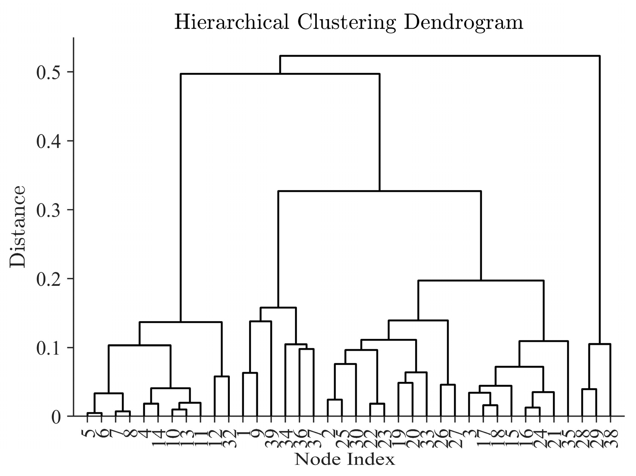
Clustering is performed using a hierarchical clustering algorithm based on the modified electrical distance matrix ED, where the electrical distance $d_{n,n^{\prime }}^{\prime }$between two nodes is defined by (15).

This paper adopts a bottom–up agglomerative algorithm. Initially, each node in the system is treated as a distinct cluster. The algorithm iteratively merges the pair of clusters with the smallest inter-cluster distance until all nodes are aggregated into a single cluster. For clustering analysis, Ward’s linkage algorithm is employed to minimize variance during merging.

Define the coupling index between nodes and partitions $X_l$:

$$X_l={\displaystyle \frac{1}{N_l}}{\sum }_{x,y\in {\Omega }_l}{d}_{xy}^{\prime }$$

(16)

The smaller its value indicates the higher the coupling of nodes within the partition; N_l is the number of nodes in the lth partition, $l=\mathrm{1,2},3,\cdots ,L$; L is the total number of partitions, $x=\mathrm{1,2},3,\dots ,N_l$, $y=\mathrm{1,2},3,\dots ,N_l;{ \Omega }_l$ is the lth partition; and$d_{xy}^{\prime }=\left(\sum _{k=1}^K{\gamma }_x^{\left(k\right)}{d}_{xy}\right)/K$.

Define coupling index $Y_l$ for different subintervals:

$$Y_l={\displaystyle \frac{10}{R}}{\sum }_{r=1}^R{\displaystyle \frac{{\sum }_{w,e\in {\Omega }_r}{d}_{we}^{\prime }}{N_r}}$$

(17)

It denotes the weighted average of the electrical distances between the partitions bordering the lth partition, and the larger the value indicates the higher the coupling between the lth partition and the neighboring partitions; R is the total number of partitions bordering the lth partition; ${\Omega }_r$ is the rth bordering partition; N_r is the total number of nodes in the rth bordering partition; and $d_{we}^{\prime }=\left(\sum _{k=1}^K{\gamma }_w^{\left(k\right)}{d}_{we}\right)/K$, $w=\mathrm{1,2},3,\dots ,N_r$, $e=\mathrm{1,2},3,\dots ,N_r$.

Combining (16) and (17), define the total regional coupling degree metric P that considers node–region coupling and region–region coupling, which is better than the coupling index proposed in [3,18]:

$$P={\sum }_{l=1}^L{X}_l+{\displaystyle \frac{1}{Y_l}}$$

(18)

Lower X_l, which means tighter intra-region coupling, and higher Y_l, which means stronger inter-region separation, will make P lower. If X_l increases or Y_l decreases, then index P will rise sharply. It reflects the comprehensive integration of coupling degrees within partitions and decoupling levels between regions. The larger the total evaluation index P of the regional coupling degree, the more effective the zoning is. However, P is susceptible to extreme X_l and Y_l, which is where attention should be paid.

After completing the clustering process, the number of partitions is initially set to two. This involves selecting a merging distance in the hierarchical clustering algorithm that divides all grid nodes into two clusters. The hierarchical clustering algorithm employed in this study follows a bottom–up agglomerative approach. When a larger merging distance is chosen for regional partitioning, individual nodes in the power grid are automatically assigned to their corresponding partitions. Concurrently, the total regional coupling index P is calculated for each partition configuration. As the number of partitions increases, the variation in P is monitored. The optimal number of partitions is determined when P reaches a local minimum, indicating the most stable coupling structure. In this case, the coupling within the region has a higher value, and the coupling between the regions has a smaller value, which is a best compromise for both within and outside the region.

Subsequently in this paper, the modified electrical distance matrix ED is reduced to two dimensions, which represent the two directions with the highest variance in the (N − 1)-dimensional vector space consisting of the entire electrical distance matrix. And, finally, the obtained partitioning results are visualized.

4. Reactive Power Partitioning Method Considering Source–Load Correlation and Regional Coupling Degree

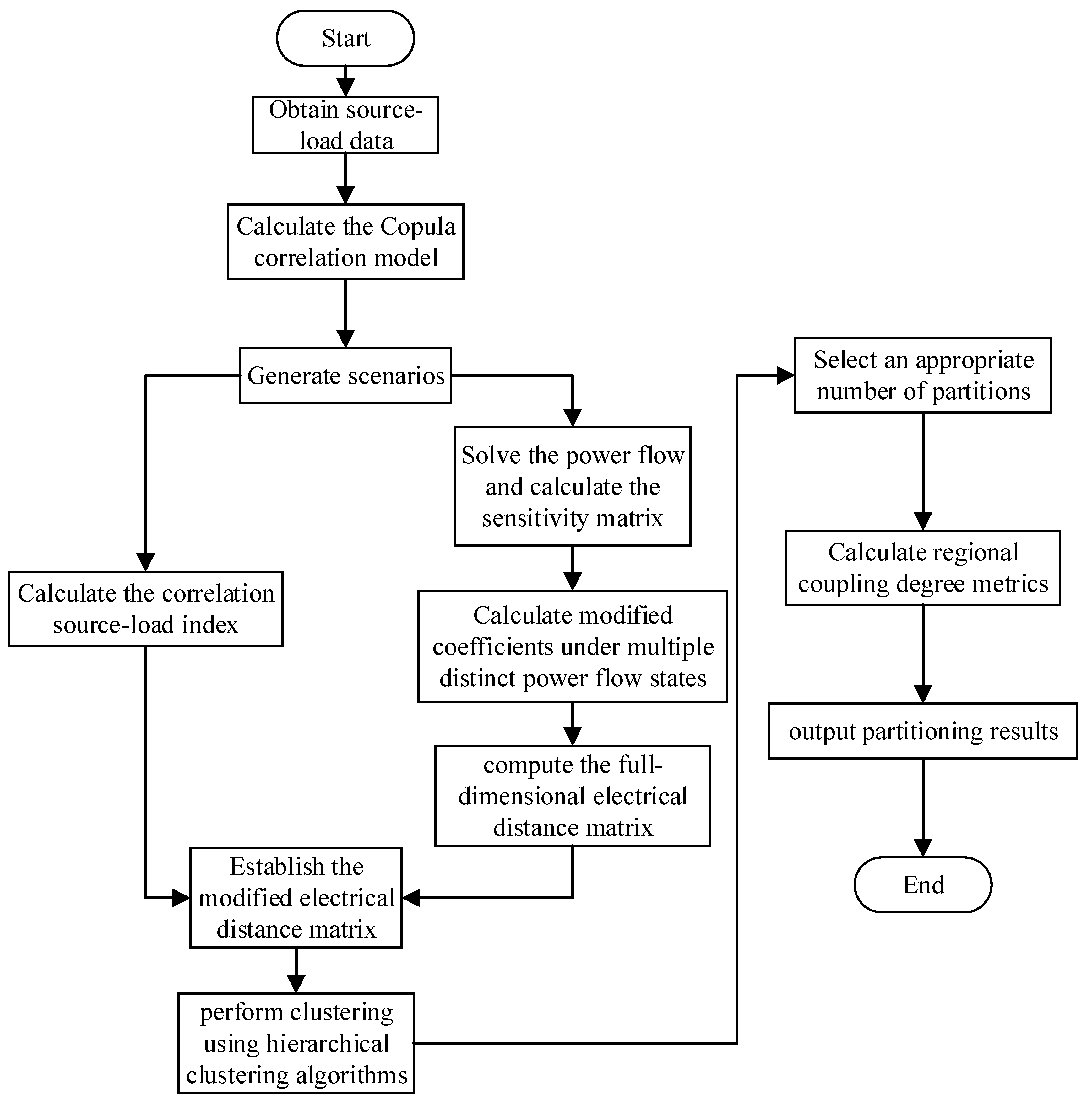
Combining the above calculation methods in this paper, the reactive power partitioning method considering the source–load correlation and regional coupling degree is composed in this paper, and the specific steps are as follows:

Step 1: Obtain the output data of all grid-connected renewable energy sources equipment and the electricity consumption load data on the user side within the power grid to be partitioned. These data are referred to as source–load data. The resolution of the source–load data used in this paper is 1 h.

Step 2: Fit the source–load data. Calculate the marginal distribution of the source–load data and construct a Gaussian Copula-based correlation model for the source–load data based on their marginal distributions.

Step 3: Use the Copula model constructed in Step 2 to generate base scenarios, and then cluster these base scenarios into K scenarios using the K-means clustering algorithm.

Step 4: Calculate the index J according to Equations (4)–(7).

Step 5: Compute the power flow for the K generated scenarios to obtain K power flow operating states, and determine the correction factor and the full-dimensional electrical distance matrix based on Equations (8)–(14).

Step 6: Based on the calculation results from Steps 4 and 5, compute the modified full-dimensional electrical distance matrix that accounts for source–load correlations.

Step 7: Perform hierarchical clustering.

Step 8: Select the number of partitions.

Step 9: Calculate the regional coupling degree metrics according to Equations (16)–(18).

Step 10: Output the partitioning results.

The flowchart of the reactive power partitioning method considering the source–load correlation and regional coupling degree is shown in Figure 1.

5. Arithmetic Analysis

For this example, we utilized source–load data including wind power, photovoltaic (PV) generation, and load data from a region in Jiangsu Province, China, with a 1 h temporal resolution.

In this paper, the computing platform we use is MATLAB R2023a under AMD Ryzen 7 5800H. It required 1.23 s for scene generation and clustering, 0.02337 s for hierarchical clustering, and 15.221086 s for parallel calculation to correct the electrical distance matrix, while the computational workflow in Reference [17] took 20 s to complete. The calculation of this method mainly focuses on the steps of generating the sensitivity matrix, but the overall speed is still very impressive. Compared with the existing methods, this method has the characteristics of a faster calculation time and better results.

For this example, the output data of all new energy-generating equipment in the grid to be partitioned and the consumer-side electric load data, referred to as source–load data, are obtained for a period of 1 h. The parameter distributions of Weibull and beta distributions are shown in Figure 2.

Subsequently, the source–load data are fitted to obtain their marginal distribution. According to [19,20,21], the daily solar irradiance, load, and wind speed distributions, respectively, follow the beta distribution, normal distribution, and Weibull distribution. We calculate the marginal distribution functions of the original data using the method of undetermined coefficients.

Based on Equations (1) and (2) and the marginal distributions, we determined the required parameters of the Gaussian Copula function using the undetermined coefficients method, thereby establishing a Gaussian Copula-based correlation model for source–load dependencies.

By sampling from the Copula model fitted to the marginal distributions, we generated 1000 initial scenarios.

The scenarios were reduced using the K-means clustering algorithm. The K-means clustering algorithm was used to reduce the 1000 original scenarios to 16 scenarios, with the probabilities of each scenario being, in order, 0.056, 0.040, 0.052, 0.048, 0.059, 0.037, 0.04, 0.038, 0.043, 0.071, 0.054, 0.048, 0.06, 0.062, 0.040, 0.049 and 0.040

Table 1. The impact of choosing the number of clusters on the system performance.

Cluster Number	P
8	19.8927
16	19.8903
20	19.8895

shows the impact of choosing the number of clusters on the system performance.

We can easily observe that, although the index P obtained by the optimal clustering determined by the elbow method is not the smallest, when the number of clusters exceeds this value, the growth trend of index P becomes slow. At the same time, it should be noted that the increase in the number of clusters will generate more scenarios, and the calculation of scenarios is very time-consuming. So, let K = 16 is a good choice.

The source–load correlation indices were calculated. PV generation units conforming to the Copula model were connected to Node 35 as PV nodes, and wind power generation units were connected to Node 38. The node system is shown in Figure 3. The system-wide source–load correlation indices under these eight scenarios were computed after integrating the renewable energy units.

Power flow calculations were performed. Power flow was simulated for the generated scenarios, yielding eight distinct power flow operating states. For each scenario, the PV plant, wind farm, and load data at sampled time instants were assigned to their respective locations, and the corresponding power flow was computed.

Clustering was performed using the hierarchical clustering algorithm. The obtained clustering results are shown in Figure 4.

As illustrated in Figure 5, the total regional coupling index P varies with the number of partitions, according to the methodology outlined in Section 3. A distinct local minimum emerges when the partition count reaches six, which aligns with the optimal configuration for minimizing inter-regional dependencies. Consequently, the final number of partitions is determined as six.

Subsequently in this paper, the modified electrical distance matrix is reduced to two dimensions, which represent the two directions with the largest variance in the (N − 1)-dimensional vector space consisting of the entire electrical distance matrix. And, finally, the obtained partitioning results are visualized. The obtained results are shown in Figure 6.

The number of hierarchical clusters we obtain through our method also meets the principle, which is mentioned in [22], that the upper limit of the number of reasonable optimal cluster partitions is $\sqrt{\mathrm{N}}$.

The source–load correlation index and the regional coupling degree index together constitute the evaluation index of the reactive power zoning for this project, and calculate the result. A comparative analysis is conducted between the partitioning results obtained through our method and those derived from the approach in [17], which are shown in

Table 2. Results of evaluation index and comparison to the results of evaluation index in reference [17].

Zone	Results of Evaluation Index in Paper				Results of Evaluation Index in Reference [17]
	${\mathit{X}}_{\mathit{l}}$	${\mathit{Y}}_{\mathit{l}}$	P	J	${\mathit{X}}_{\mathit{l}}$	${\mathit{Y}}_{\mathit{l}}$	P
1	0.6340	0.2798	19.8903	0.5107	0.3418	0.3290	20.7750
2	0.3571	0.3352			0.3699	0.3196
3	0.1621	0.3742			0.3571	0.3590
4	0.3409	0.3384			0.2600	0.4242
5	0.1949	0.3676			0.6279	0.2708
6	0.3439	0.3378			0.1954	0.2763

. The results of the six zones are shown in

Table 3. Partitioning results.

Zone	Nodes Included in the Partition
1	34, 36, 37
2	1, 9, 39
3	3, 15–18, 21, 24, 35
4	2, 19, 20, 22, 23, 25–27, 30, 33
5	4–8, 10–14, 31, 32
6	28, 29, 38

.

From the results in Table 2, it is evident that under the partitioning method proposed in this paper, the coupling degree between nodes and partitions is smaller compared to that in [17], with mean values of 0.3390 and 0.3587, respectively. Additionally, the inter-regional coupling indicators are also lower than those in [17], resulting in an overall smaller total coupling degree for the proposed method.

The resultant data in Table 3 indicate that the source–load correlation index obtained through this partitioning method is relatively low. Additionally, the regional coupling degree index is also small within each partition. These results suggest that the coupling between various nodes within each partition is strong, and the overall regional coupling is satisfactory. Therefore, the partitioning results are deemed to be more reasonable.

To quantitatively evaluate the rationality and advancement of the proposed method, this study introduces the regional reactive power imbalance index as an additional evaluation metric alongside the regional coupling degree. A comparative analysis is conducted between the partitioning results obtained through our method and those derived from the approach in [5,17].

The definition of the regional reactive power imbalance index is as follows:

$$\eta =\sqrt{{\displaystyle \frac{1}{L}}{\sum }_{l=1}^L\left({\tau }_l-\overline{\tau }\right)}$$

(19)

$${\tau }_l={\displaystyle \frac{Q_l^G-Q_l^L}{Q_l^G}}$$

(20)

where ${\tau }_l$ is the reactive power reserve of partition l; $\overline{\tau }$ is the mean absolute value of reactive power reserves across L partitions; $Q_l^G$ is the sum of the maximum reactive power outputs of all reactive power sources in partition l; and $Q_l^L$ is the total reactive load in partition l. η represents the regional reactive power imbalance index. Its physical significance lies in measuring the balance level of reactive power sources across partitions in the post-partitioning system. A smaller value indicates more rational allocation of reactive power sources and higher resource utilization efficiency.

Comparison results are shown in

Table 4. Results of reactive power imbalance index.

Method	$\mathit{\eta }$	$\overline{\mathit{\tau }}$/%
This paper	0.25925	56.372
Reference [17]	0.29156	54.185

.

The data in Table 4 further validate the rationality of the partitioning approach presented here, as evidenced by the well-balanced reactive power reserves. A comparative analysis shows that the proposed partitioning method achieves a lower regional coupling degree, reducing it by 4.216% compared to reference [17], while also decreasing the regional reactive power imbalance by 11.082%. This effectively enhances intra-regional connectivity and reduces inter-regional reactive power dependency, thereby ensuring the local reactive power balance within each partition.

After the above partition is completed, in order to further partition the effectiveness, we consider the new energy output scenario as shown in

Table 5. Imbalance index under different renewable energy sources output.

	0.1 × Pv and 0.1 × Pw	0 × Pv and 0 × Pw	Pv and Pw
This Paper	0.38736	0.41528	0.28447
Reference [17]	0.35985	0.37883	0.33500

and calculate the imbalance index under the corresponding scenario.

It is not difficult to see from Table 5 that the new energy output gradually decreases with the new energy output, and the imbalance is constantly increasing, which is obvious. At the same time, when the new energy fluctuation range is large, the degree of imbalance brought by the proposed zoning is higher than that of reference [17], which indicates that the internal balance of the zoning obtained by the proposed method is closer.

6. Conclusions

This paper addresses the challenges posed by the expanding integration of renewable energy and enhanced power system interconnectivity, and we propose a dynamic reactive power partitioning method that integrates Copula-based source–load correlation and composite coupling metrics. A multidimensional partitioning criterion is established by combining time-series correlation indices of source–load interactions with an evaluation framework for regional electrical coupling. The implementation involves constructing a modified electrical distance matrix that accounts for power fluctuations in renewable generation units. Dynamic coupling relationships are modeled by incorporating time-series correlation analysis between the source and load. A spectral clustering algorithm is applied to solve the optimized partitioning model. The resulting partition achieves strong electrical coupling between nodes and regions. This method provides effective zoning boundaries for reactive power and voltage optimization control. It enhances system operational economy and voltage stability through rational regional decoupling.

The effect of reactive power partitioning is to achieve the purpose of reactive power optimization, which is conducive to the realization of the local balance of reactive power and the accurate control of node voltage. This method is a scientific and easy-to-implement multi-objective reactive power optimization method in a power system, which is widely applicable to power networks, has significant engineering practical value, and has a wide range of application prospects.

Our case studies demonstrate a 4.216% reduction in the regional coupling degree metric and an 11.082% improvement in the regional reactive power imbalance. However, the Gaussian Copula’s limitations in capturing tail dependencies warrant further investigation.

7. Patents

Patent name: the invention relates to a reactive power partitioning method considering source charge correlation and region coupling degree.

Application number: CN202411358207.6.

Application date: 2024.9.27.