Online Identification of Differential Order in Supercapacitor Fractional-Order Models: Advancing Practical Implementation

Abstract

Supercapacitors (SCs) are increasingly recognized as a reliable energy storage solution in various industrial applications due to their high power density and exceptionally long lifespan. SC-powered systems demand precise parameter identification to enable effective energy management. Although various approaches exist for the offline identification of SCs, some parameters depend on factors such as state of health (SoH), aging, temperature, and their combination. Consequently, the variation in parameter values under different conditions highlights the importance of online identification based on a dynamic model structure. Among various SC models proposed in the literature, fractional-order models offer greater accuracy, making them a superior choice for SC modeling. However, the conventional formulation in these models requires a very long window of samples and coefficients for filter implementation. Additionally, due to the several orders of magnitude difference in the elements of matrices, numerical instability can arise, leading to errors and drift in the final calculations. In this paper, a novel online identification approach is introduced for differential order estimation in fractional-order SC models. The proposed method significantly shortens the long window while maintaining accuracy, making it feasible for implementation in low-cost microcontrollers and a viable solution for real-world applications. In addition, the proposed method addresses the drift error by applying online least squares error estimation that aligns it with its offline estimated value.

1. Introduction

Today, with the growing adoption of renewable energy sources and electric vehicles, the significance of Electrochemical Energy Storage Systems (EESSs) has seen a dramatic increase. Prominent EESSs include rechargeable batteries [1], fuel cells, and supercapacitors (SCs). SCs uniquely bridge the gap between traditional capacitors and batteries in terms of energy density and power density. While batteries provide high energy density compared to SCs, their power density is inadequate, and thus SCs fill this intermediate niche, making them an unparalleled choice for applications that require high power density [2]. As a real-world application, the Lamborghini Sián FKP 37, a hybrid electric super sports car, utilizes a supercapacitor bank as its energy storage system [3].

SCs are known for their exceptionally long lifespan, wide operational temperature range, durability in harsh environments, efficient cycling capabilities, and low maintenance costs. These attributes have made them indispensable in various industries, from transportation to renewable energies [4].

SCs play a crucial role in Hybrid Energy Storage Systems (HESSs). To optimize performance, extend lifespan, reduce costs, and minimize environmental impact, ESSs often integrate multiple storage technologies. These hybrid ESSs are utilized across various applications [5]. A key characteristic of HESSs is their high-power capability, which is typically achieved through the incorporation of SCs. These components offer exceptional cycling durability (approximately half a million cycles [6]) and remarkable power densities (500–5000 W/kg [7]). SC applications span a wide range of fields, including regenerative braking in railways, electric buses, forklifts, and pitch control systems in wind turbines [2,8].

Precise modeling and parameter identification are crucial for the energy management, thermal regulation, power control, safety monitoring, and health assessment of SCs. Equivalent circuit models (ECMs) are widely used for these tasks due to their structural simplicity and computational efficiency, making them effective for SOC estimation [9], charging control [10], and SOH prediction [11]. The accuracy of SOC and SOH estimation depends on both the fidelity of the supercapacitor model and the effectiveness of the estimation algorithm. Since SOC estimation relies on the observer accuracy, and the observer performance is directly tied to the accuracy of the model, precise real-time parameter updates are essential to account for aging effects [12]. Supercapacitor degradation is typically assessed by an increase in internal resistance or a decrease in equivalent capacitance, both of which strongly correlate with the state of health (SOH) [13]. There are three main modeling categories for EESSs:

• Physics-based, which uses electrochemical analysis to explain the dynamics [14,15].
• Data-driven, which uses impedance spectroscopy and frequency-domain analysis to identify the model [16,17].
• Equivalent circuit, which is the most popular approach in practice because of its simplicity and acceptable accuracy [18,19,20,21,22,23,24,25,26,27].

SC dynamics models can be classified into either integer- or fractional-order models [18]. An analytical study in [14] demonstrates that fractional-order models are more effective in capturing SC dynamics. In [19], a comparison study on the accuracy of various integer-order and fractional-order models was conducted, showing that fractional-order models provide 15–30% greater accuracy compared to integer-order ones, making them superior for the modeling of SCs [20]. As demonstrated in [28], a fractional-order model is equivalent to an Lth-order ECM, where L represents an adjustable memory length. This means that a fractional-order model, despite having a fixed number of model parameters, can achieve the same level of accuracy as an ECM of any order.

Several ECMs for EESSs and in particular SCs are discussed in the literature, with model complexity varying based on the application. While more complex models tend to offer higher accuracy, they also introduce greater challenges in parameter identification and lack practicality. As a result, there is an inherent engineering trade-off between achieving model accuracy and maintaining the feasibility of robust state estimation [20].

A literature review on parameter identification was conducted in [29], where SC parameter identification was broadly categorized into online and offline methods. Online identifications primarily rely on regularization techniques such as least squares estimation (LSE) [30], recursive least squares estimation (RLSE) [26,31,32,33,34,35,36,37], state-estimation-based methods [12,13], Lyapunov-based observers [38], and gradient-based methods [39,40,41]. In contrast, offline identifications employ global optimization techniques, such as Genetic Algorithms (GAs) and Particle Swarm Optimization (PSO), as demonstrated in [24,42,43]. As an example, ref. [21] has performed the primary offline identification based on global optimization methods and online corrections using the subspace system identification algorithm.

Offline identification typically uses voltage, current, and SoC to determine the model coefficients. However, SC parameters can also be influenced by factors such as SoH, aging, temperature, and their combinations, and discharge mode [44] which are not considered in the offline calculation stage. Therefore, any estimation based on fixed coefficients from offline identification may lead to drift over time as the SC ages or operates in different environmental conditions. This is where online estimation becomes essential, dynamically adjusting the coefficients to enhance accuracy. As fractional-order SC models offer 15–30% greater accuracy than integer-order models [39], they are a more effective choice for SC modeling. However, the online identification of the fractional order in SCs is not straightforward and presents several challenges. As derived in [39], a procedure for determining the optimal differential order using a descent-gradient method requires infinite memory for implementation. Additionally, the formulation exhibits drift errors in practice due to ill-conditioned matrix inversions.

The proposed modification to the conventional algorithm structure is shown in Figure 1. The structure of this paper is as follows:

• Section 2 reviews the ECM and the governing equations for an SC. Subsequently, the voltage dynamics are derived, and based on this, the LSE for online parameter identification is formulated.
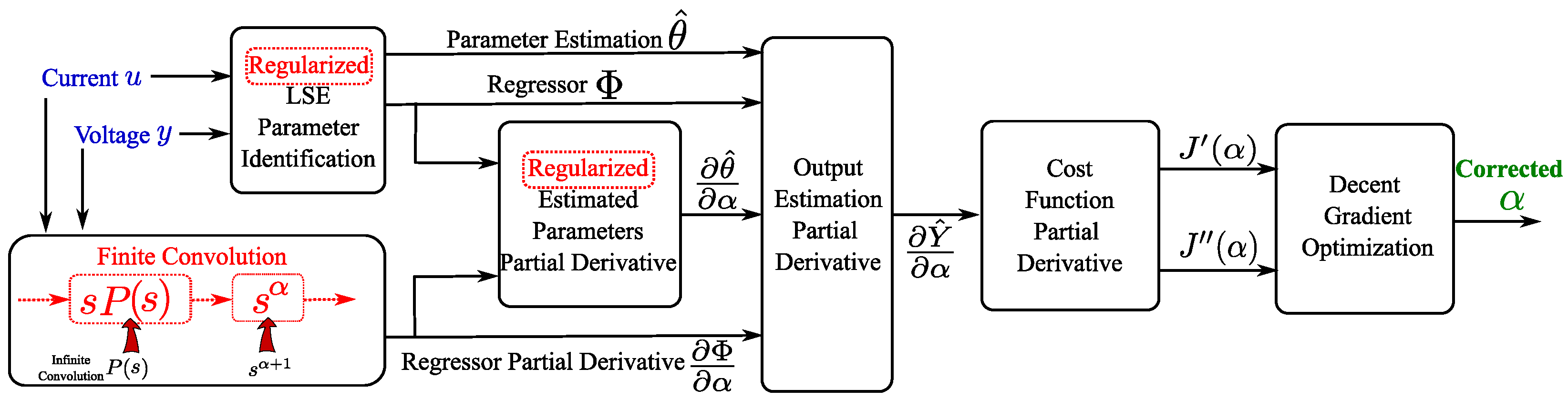
• While Section 2 assumes the differential order to be known, it must be updated over time using a longer sample period. Therefore, in Section 3, the LSE equation is utilized to derive a descent-gradient identification method for the fractional order. Since implementing an infinite filter convolution is required at this stage, the proposed formulation for truncating the convolution is introduced in this section.
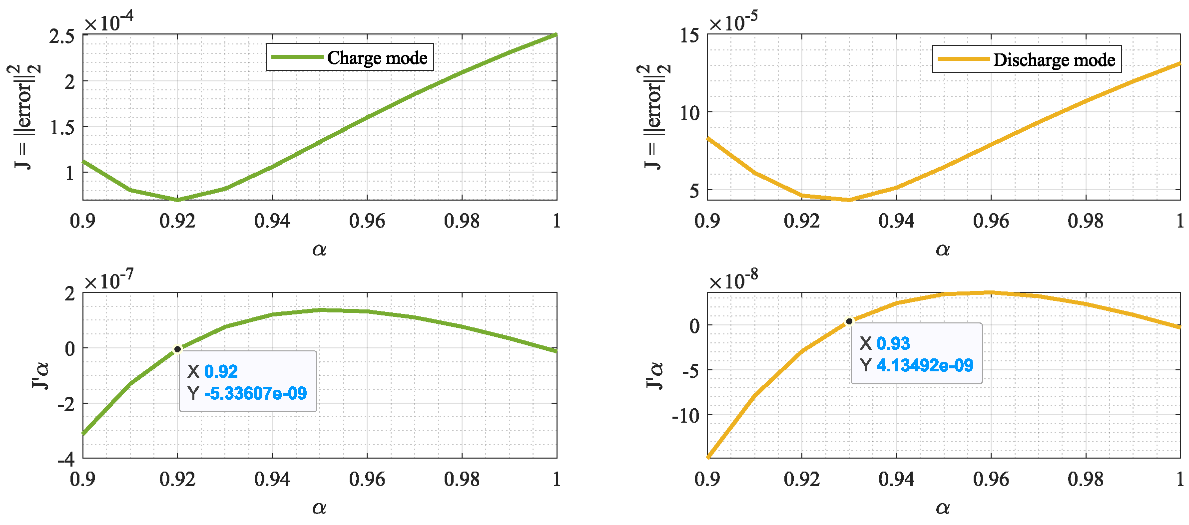
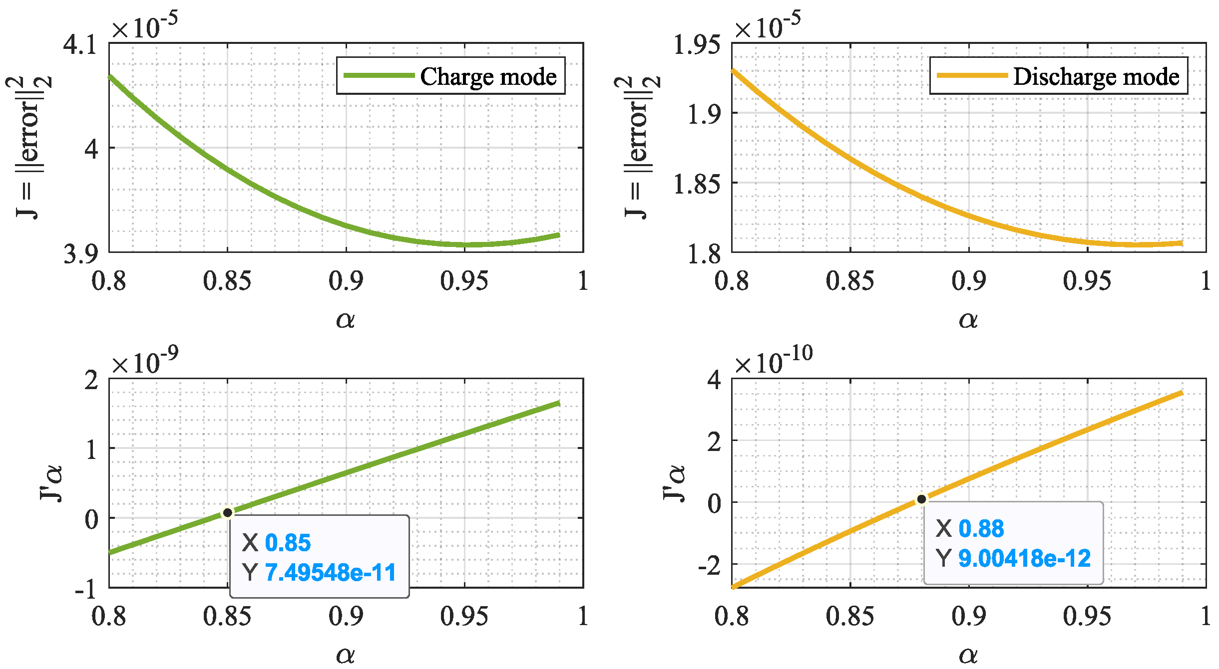
• Since any error in the online estimation of parameters leads to errors in the estimation of the differential order, a regularized formulation is introduced in Section 4 to reduce the error in determining the optimal differential order. It is shown that this approach increases the alignment between the minimum of the cost function and the zero crossing of its derivative.
• To validate the accuracy and effectiveness of the proposed parameter identification methodology, a series of experiments was conducted, with the results presented and discussed in Section 5.

2. Parameter Identification Using Voltage Dynamics

To determine the optimal differential order, the other model parameters must first be identified using online LSE. In this paper, only the voltage dynamics are considered, as the primary focus is on refining the differential order formulation. Figure 2 demonstrates the fractional-order ECM of the SC. In this ECM, the inductance of the current collector and SC casing is neglected due to its minimal value. Its impact is only significant at high frequencies, which are beyond the scope of this study. As highlighted in [20], which provides a comprehensive collection of various battery and supercapacitor models, inductance is not considered in any of them. This omission indicates that its effect is negligible within the practical frequency range.

By applying Kirchhoff law, it can be concluded that

$$\begin{array}{c}\hfill \left\{\begin{array}{cc}\hfill i_1\left(t\right)& ={\displaystyle \frac{v_1\left(t\right)}{R_1}}+C_1{\displaystyle \frac{d^{\alpha }{v}_1\left(t\right)}{d{t}^{\alpha }}}\hfill \\ \hfill i_1\left(t\right)& =i\left(t\right)-{\displaystyle \frac{v_1\left(t\right)}{R_2}}-{\displaystyle \frac{E_0}{R_2}}\hfill \\ \hfill v_1\left(t\right)& =v_T\left(t\right)-E_0-R_{0}i\left(t\right)\hfill \end{array}\right.\end{array}$$

(1)

where $C_1$ is the Constant Phase Element (CPE), $\alpha$ is the fractional order of the CPE, the $R_1\left|\right|C_1$ branch represents the charge redistribution and diffusion property of the SC, $R_2$ is leakage resistance, $R_0$ is Equivalent Series Resistance (ESR), $v_1\left(t\right)$ is the voltage across $C_1$, $i_2\left(t\right)$ is the leakage current, $i\left(t\right)$ and $v_T\left(t\right)$ are the terminal current and voltage, respectively. $E_0$, the Open Circuit Voltage (OCV) of the SC at a specific SOC under resting conditions can be expressed as a function of the SOC. By substituting the $i_1\left(t\right)$ and $v_1\left(t\right)$ equivalents into (1), it can be rewritten as:

$$({\displaystyle \frac{1}{R_1}}+{\displaystyle \frac{1}{R_2}}+C_1)v_T\left(t\right)=(1+{\displaystyle \frac{R_0}{R_2}}+{\displaystyle \frac{R_0}{R_1}})i\left(t\right)+\left(C_1{R}_0\right)D^{\alpha }i\left(t\right)-C_1{D}^{\left(\alpha \right)}(v_T\left(t\right)-E_0)+({\displaystyle \frac{1}{R_1}}+C_1)E_0$$

where $D^{\left(\alpha \right)}u\left(t\right)=D^{\alpha }u\left(t\right)-u\left(t\right)$. This equation can be discretized and take the following form:

$$\begin{array}{cc}\hfill v_T\left(k\right)& =y\left(k\right)={\varphi }_k^T{\theta }_k\hfill \\ \hfill {\varphi }_k& ={\left[\begin{array}{cccc}i\left(k\right)& D^{\alpha }i\left(k\right)& D^{\left(\alpha \right)}(v_T\left(k\right)-E_0)& E_0\end{array}\right]}^T\hfill \\ \hfill {\theta }_k& ={\left[\begin{array}{cccc}{\theta }_1\left(k\right)& {\theta }_2\left(k\right)& {\theta }_3\left(k\right)& {\theta }_4\left(k\right)\end{array}\right]}^T\approx {\left[\begin{array}{cccc}1/C_1& R_0& -1& 1\end{array}\right]}^T\hfill \end{array}$$

(2)

$E_0$ is expressed as a function of the SOC, defined as $E_0=h\left(SOC\right)$. The SOC can be obtained by by having the leakage resistance and SC capacity and applying Coulomb Counting [42]:

$${\displaystyle \frac{d}{dt}}SOC\left(t\right)=\eta i_1\left(t\right)=\eta (i\left(t\right)-{\displaystyle \frac{v_T\left(t\right)}{R_2}})$$

(3)

in which $\eta =1/\left(3600C_{Ah}\right)$ and $C_{Ah}=C_n{V}_n/3600$. Here, $C_n$ represents the nominal capacitance of SC, and $V_n$ denotes the nominal voltage of the SC.

By collecting $h+1$ samples, the parameter vector ${\theta }_k$ can be estimated using the LSE method as follows:

$$\begin{array}{cc}\hfill {\widehat{\theta }}_k& ={\left({\Phi }_k^{T}W{\Phi }_k\right)}^{-1}{\Phi }_k^{T}W{Y}_k\hfill \\ \hfill {\Phi }_k& ={\left[\begin{array}{cccc}{\varphi }_{k-h}& \cdots & {\varphi }_{k-1}& {\varphi }_k\end{array}\right]}^T{Y}_k={\left[\begin{array}{cccc}y(k-h)& \cdots & y(k-1)& y\left(k\right)\end{array}\right]}^T\hfill \end{array}$$

(4)

3. Differential Order Identification

The differential order $\alpha$ is first identified through offline global optimization. This value can then be used as the initial value in a descent gradient optimization. By defining the cost function as:

$$J\left(\alpha \right)=\sum _{j=k-h}^k{(y\left(j\right)-\widehat{y}(j,\alpha ))}^2=\left|\right|Y_k-{\widehat{Y}}_k{\left|\right|}_2^2$$

(5)

and applying the descent gradient optimization to the cost function, the optimum $\alpha$ can be updated in each iteration.

$${\alpha }_{k+1}={\alpha }_k-{\left({\left[J_{\alpha \alpha }^{″}+\xi I\right]}^{-1}{J}_{\alpha }^{\prime }\right)}_{\alpha ={\alpha }_k}$$

(6)

In which $\xi I$ is added for numerical stability when inverting $J^{″}$ and

$$\begin{array}{cc}\hfill J_{\alpha }^{\prime }& =-2\sum _{j=k-h}^k(y\left(j\right)-\widehat{y}(j,\alpha )){\displaystyle \frac{\partial \widehat{y}(j,\alpha )}{\partial \alpha }}=-2{(Y_k-{\widehat{Y}}_k)}^T{\displaystyle \frac{\partial {\widehat{Y}}_k}{\partial \alpha }}\hfill \end{array}$$

(7)

$$\begin{array}{cc}\hfill J_{\alpha \alpha }^{″}& =2\sum _{j=k-h}^k{\displaystyle \frac{\partial \widehat{y}(j,\alpha )}{\partial \alpha }}{\left({\displaystyle \frac{\partial \widehat{y}(j,\alpha )}{\partial \alpha }}\right)}^T=2\left|\right|{\displaystyle \frac{\partial {\widehat{Y}}_k}{\partial \alpha }}{\left|\right|}_2^2\hfill \end{array}$$

(8)

Knowing that ${\widehat{Y}}_k={\Phi }_k{\widehat{\theta }}_k$, its partial derivative with respect to $\alpha$ will be

$${\displaystyle \frac{\partial {\widehat{Y}}_k}{\partial \alpha }}={\displaystyle \frac{\partial \Phi }{\partial \alpha }}{\widehat{\theta }}_k+{\Phi }_k{\displaystyle \frac{\partial {\widehat{\theta }}_k}{\partial \alpha }}$$

(9)

where

$$\begin{array}{cc}\hfill {\displaystyle \frac{\partial {\Phi }_k}{\partial \alpha }}& ={\left[\begin{array}{cccc}{\displaystyle \frac{\partial {\varphi }_{k-h}}{\partial \alpha }}& \cdots & {\displaystyle \frac{\partial {\varphi }_{k-1}}{\partial \alpha }}& {\displaystyle \frac{\partial {\varphi }_k}{\partial \alpha }}\end{array}\right]}^T,{\displaystyle \frac{\partial {\varphi }_k^T}{\partial \alpha }}=\left[\begin{array}{cccc}0& (s^{\alpha }lns)i\left(k\right)& (s^{\alpha }lns)(v_T\left(k\right)-E_0)& 0\end{array}\right]\hfill \\ \hfill {\displaystyle \frac{\partial {\widehat{\theta }}_k}{\partial \alpha }}& ={\displaystyle \frac{\partial M_k}{\partial \alpha }}{\Phi }_k^{T}W{Y}_k+M_k{\displaystyle \frac{\partial {\Phi }_k^T}{\partial \alpha }}W{Y}_k\hfill \\ \hfill {\displaystyle \frac{\partial M_k}{\partial \alpha }}& =-M_k{\displaystyle \frac{\partial M_k^{-1}}{\partial \alpha }}{M}_k,M_k={\left({\Phi }_k^{T}W{\Phi }_k\right)}^{-1},{\displaystyle \frac{\partial M_k^{-1}}{\partial \alpha }}={\Phi }_k^{T}W{\displaystyle \frac{\partial {\Phi }_k}{\partial \alpha }}+{\displaystyle \frac{\partial {\Phi }_k^T}{\partial \alpha }}W{\Phi }_k\hfill \end{array}$$

In the above equations $F\left(s\right)=s^{\alpha }lns$ can be regarded as a signal processing filter. To apply the inverse Laplace transform to it, it can be reformulated as:

$$F\left(s\right)=s^{\alpha }s{\displaystyle \frac{lns}{s}}=s^{\alpha }sP\left(s\right)$$

(10)

where $P\left(s\right)=lns/s$. By applying the inverse Laplace transform to $P\left(s\right)$, its time-domain equivalent for the convolution operation can be obtained.

$$L^{-1}\left(P\left(s\right)\right)=L^{-1}\left({\displaystyle \frac{lns}{s}}\right)=p\left(t\right)=-ln\left(t\right)-E$$

(11)

in which E is the Euler–Mascherni constant. Regarding $u\left(t\right)$ as the input of the filter $P\left(s\right)$ and applying a convolution operation on the signal, the output of the filter is

$$w\left(t\right)={\int }_0^{t}p(t-\tau )u\left(\tau \right)d\tau$$

(12)

The discrete form of (12) can be rewritten as follows:

$$W\left(k\right)=\sum _{j=0}^{k-1}\left[{\int }_{j{T}_s}^{(j+1)T_s}p(k{T}_s-\tau )d\tau \right]u\left(j\right)=\sum _{j=0}^{k-1}c(j,k-1)u\left(j\right)$$

(13)

where

$$c(j,k-1)=\left\{\begin{array}{cc}(1-E)+(k-j-1)ln(k-j-1)-(k-j)ln(k-j)\hfill & j<k-1\hfill \\ 1-E\hfill & j=k-1\hfill \end{array}\right.$$

As can be seen, implementing the filter $P\left(s\right)$ on a signal requires infinite memory to store all the previous history of the signal, as well as an infinite processor to perform the convolution of the filter and the signal over all past time, since the coefficients c do not fade over time. However, this work proposes a formulation to address and overcome this challenge. For the next sample, since $c(j,k)=c(j-1,k-1)$, it can be rewritten as

$$\begin{array}{cc}\hfill W(k+1)& =\sum _{j=0}^{k}c(j-1,k-1)u\left(j\right)\hfill \end{array}$$

(14)

By utilizing one degree of differentiation to truncate the infinite convolution series, the filter transforms from $P\left(s\right)$ to $sP\left(s\right)$. In discrete form, differentiating $W\left(k\right)$ yields:

$$\begin{array}{cc}\hfill \Delta W(k+1)& =W(k+1)-W\left(k\right)=\sum _{j=0}^{k}c(j-1,k-1)u\left(j\right)-\sum _{j=0}^{k-1}c(j,k-1)u\left(j\right)\hfill \\ \hfill & =\sum _{j=0}^{k-1}(c(j-1,k-1)-c(j,k-1))u\left(j\right)+c(k-1,k-1)u\left(k\right)\hfill \end{array}$$

(15)

Now the coefficients of the series fade over time and their limit approaches zero because

$$\begin{array}{cc}\hfill & \underset{(k-j)\to \infty }{lim}(c(j-1,k-1)-c(j,k-1))=\hfill \\ \hfill & \underset{(k-j)\to \infty }{lim}ln{\displaystyle \frac{{(k-j)}^{2(k-j)}}{{(k-j+1)}^{(k-j+1)}{(k-j-1)}^{(k-j-1)}}}=\underset{(k-j)\to \infty }{lim}ln{\displaystyle \frac{{(k-j)}^{2(k-j)}}{{(k-j)}^{(k-j+1)}{(k-j)}^{(k-j-1)}}}=0\hfill \end{array}$$

Hence, it is sufficient to calculate $\Delta W\left(k\right)$ only for the latest samples. Consequently, the implementable filter $sP\left(s\right)$ for the signals is given as follows:

$$\begin{array}{cc}\hfill & \Delta W(k+1)\approx \sum _{j=k-h}^{k-1}(c(j-1,k-1)-c(j,k-1))u\left(j\right)+c(k-1,k-1)u\left(k\right)=\sum _{j^{\prime }=0}^{h}d\left(j^{\prime }\right)u\left(j^{\prime }\right)\hfill \end{array}$$

(16)

In which h is the truncation horizon, $j^{\prime }$ denotes the latest sample, and

$$d\left(j^{\prime }\right)=\left\{\begin{array}{cc}c(j^{\prime }-1,h-1)-c(j^{\prime },h-1)\hfill & j^{\prime }<h\hfill \\ 1-E\hfill & j^{\prime }=h\hfill \end{array}\right.$$

(17)

In conclusion, this section proposed calculating the output of the filter $sP\left(s\right)$ as a whole instead of calculating the output of the filter $P\left(s\right)$ to overcome the challenge of the infinite convolution.

The derivative formulation is validated by sweeping $\alpha$ and observing J along with its proposed derivative $J^{\prime }\left(\alpha \right)$. Figure 3 confirms that the sign of $J^{\prime }\left(\alpha \right)$ aligns with the slope of J when $\theta$ is considered fixed. Hence, the formulation performance is verified.

However as it is depicted in Figure 4, when $\theta$ is estimated using online LSE, a drift error emerges, causing a mismatch between the minimum point of J and the zero crossing of ${\displaystyle \frac{\partial J}{\partial \alpha }}$. This error is primarily caused by inaccuracies in inverting the M matrix when its condition number is large.

4. Decreasing Optimum Point Drift Error

As shown in the previous section, the proposed algorithm demonstrates promising performance when $\theta$ is assumed to be fixed. However, it must also be effective when $\theta$ is estimated dynamically. In cases where $\theta$ is estimated using online LSE, a drift emerges between the minimum point of J and the zero crossing of $\partial J/\partial \alpha$. To overcome this mismatch and eliminate the drift, a regularized estimation of $\theta$ can be employed. Since the error in $\theta$ arises from inaccuracies in inverting M, the condition number of M can be improved using the following estimation method:

$$\begin{array}{cc}\hfill {\widehat{\theta }}_k& ={\theta }_0+{({\Phi }_k^{T}W{\Phi }_k+\lambda I)}^{-1}{\Phi }_k^{T}W(Y_k-{\Phi }_k{\theta }_0)\hfill \end{array}$$

(18)

Here, $\lambda I$ is added to M for numerical stability during inversion. $\lambda$ is a small arbitrary number (set to 1 in this case), and I represents the $2\times 2$ identity matrix. The constants in ${\theta }_0$ are determined using offline identification methods. For offline identification, a pulse train current is applied for 1 min, followed by a 279 min rest period, during which the voltage is measured. The recorded voltage and current data are then utilized in nonlinear gray-box identification toolboxes to estimate the model parameters [42]. However, offline identification is beyond the scope of this work. Figure 5 demonstrates that the drift between the minimum point of J and the zero crossing of its derivative is significantly reduced after applying the formulation (18).

Given that ${\widehat{Y}}_k={\Phi }_k{\widehat{\theta }}_k$, its partial derivative with respect to $\alpha$ is expressed as:

$${\displaystyle \frac{\partial {\widehat{Y}}_k}{\partial \alpha }}={\displaystyle \frac{\partial \Phi }{\partial \alpha }}{\widehat{\theta }}_k+{\Phi }_k{\displaystyle \frac{\partial {\widehat{\theta }}_k}{\partial \alpha }}$$

(19)

where

$$\begin{array}{cc}\hfill {\displaystyle \frac{\partial {\widehat{\theta }}_k}{\partial \alpha }}& =({\displaystyle \frac{\partial M_k}{\partial \alpha }}{\Phi }_k^T+M_k{\displaystyle \frac{\partial {\Phi }_k^T}{\partial \alpha }})W(Y_k-{\Phi }_k{\theta }_0)+M_k{\Phi }^{T}W(-{\displaystyle \frac{\partial {\Phi }_k}{\partial \alpha }}{\theta }_0)\hfill \\ \hfill {\displaystyle \frac{\partial M_k}{\partial \alpha }}& =-M_k{\displaystyle \frac{\partial M_k^{-1}}{\partial \alpha }}{M}_k,M_k={({\Phi }_k^{T}W{\Phi }_k+\lambda I)}^{-1},{\displaystyle \frac{\partial M_k^{-1}}{\partial \alpha }}={\Phi }_k^{T}W{\displaystyle \frac{\partial {\Phi }_k}{\partial \alpha }}+{\displaystyle \frac{\partial {\Phi }_k^T}{\partial \alpha }}W{\Phi }_k\hfill \end{array}$$

5. Experimental Results

5.1. Test Setup

A 58000mF 16.2v, Maxwell Technologies (San Diego, CA, USA) supercapacitor was employed to validate the proposed approach in an experimental environment. The experimental setup included the necessary measurement instruments for applying the input current and capturing the output voltage, ensuring accurate data collection for state estimation analysis, as summarized in

Table 1. Test setup instruments.

Instrument	Brand	Model	Communication
Power Supply	Xantrex (San Diego, CA, USA)	XT 60-1	GPIB
Electronic Load	Chroma (Wu-Ku, Taiwan)	6314-63102	GPIB
Multimeter	Keithley (Cleveland, OH, USA)	2700	GPIB

. As in [45], the data acquisition was performed using specialized devices connected via a GPIB interface. Figure 6 illustrates the installation of the experimental test setup. The supercapacitor used in the experimental setup was a Maxwell BMOD0058 E016 B02 module (Maxwell Technologies, San Diego, CA, USA) consisting of six BCAP0350 E270 T11 cells (Maxwell Technologies, San Diego, CA, USA) connected in series, with each cell rated at 350 Farads and 2.7v.

The offline-identified values of parameters are shown in

Table 2. The parameters of equivalent circuit model.

Parameter	Charge Value	Discharge Value	Unit
$R_1$	31	8.3	MΩ
$R_2$	23	60.8	kΩ
$R_0$	14	28	mΩ
$C_1$	415	821	F
$C_{Ah}$	286	233	mAh

.

And $h\left(SOC\right)$ can be expressed as a polynomial as follows:

$$\begin{array}{cc}\hfill h\left(SOC\right)& =\left[\begin{array}{cccccc}{a}_5& a_4& a_3& a_2& a_1& a_0\end{array}\right]\hfill \\ \hfill & \times {\left[\begin{array}{cccccc}SO{C}^5& SO{C}^4& SO{C}^3& SO{C}^2& SOC& 1\end{array}\right]}^T\hfill \end{array}$$

The identified constants $a_i$ for the test step in charging and discharging modes are shown in

Table 3. The constants of $h\left(SOC\right)$.

Parameter	${\mathit{a}}_5$	${\mathit{a}}_4$	${\mathit{a}}_3$	${\mathit{a}}_2$	${\mathit{a}}_1$	${\mathit{a}}_0$
Charge	0	−0.675	1.798	−5.23	19.9	−0.0282
Discharge	−9.67	33.95	$-4$2.1	21.09	10.2	−0.012 + $a_0^{\prime }$

; in which $a_0^{\prime }$ is a calibration constant that can be calculated by matching the $E_0$ value and $h\left(SOC\right)$ at the start of the discharging mode.

5.2. Test Procedure

Sawtooth Charging and Discharging Mode:

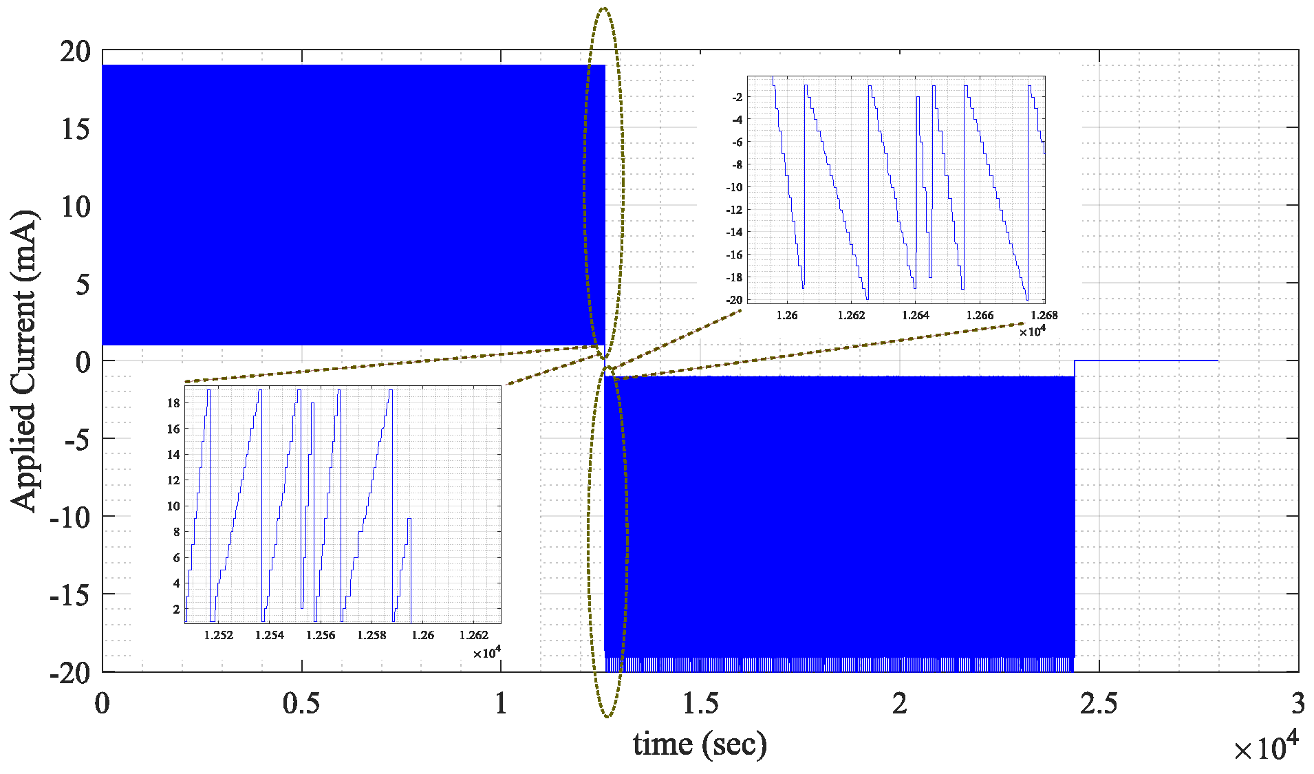
• Current Injection: A repetitive sawtooth current with a fixed amplitude of 20 mA was injected into the SC. The waveform rising time was swept in each repetition, with values of 5 s, 10 s, 15 s, and 20 s. The variation in the period was intended to enrich the signal inputs and improve the conditioning of the matrix in the LSE. A richer signal leads to a more accurate estimation. This small-amplitude current can be superimposed onto the main current solely for system identification. In other words, any rich-signal current can be utilized for this purpose. The waveform of the applied current is depicted in Figure 7. The values of voltage, current, and their time stamp were recorded with a sample time of 1 s.
• Current Draw: Similar to the previous stage, a repetitive sawtooth current with an amplitude of 20 mA was drawn from the SC, with a variable rising time, aiming to reduce the SC bank voltage from 10 V to 8 V. The voltage, current, and corresponding timestamps were recorded at a sampling interval of 1 s.
• Resting Mode: The voltage across the SC bank was recorded for 60 min during the rest period.

5.3. Test Results

Figure 8a illustrates that the online estimate of $\alpha$ successfully converges to its optimal value for both charge and discharge modes when $\theta$ is fixed. However, in Figure 8b, when $\theta$ is estimated using conventional LSE, a mismatch appears between the optimal and converged values. This mismatch is significantly reduced using regularized LSE, as shown in Figure 8c. The optimal and converged values for different cases are presented in

Table 4. Optimal values and converged values of $\alpha$.

Case	Charge Mode		Discharge Mode
	Optimal Value	Converged Value	Optimal Value	Converged Value
Constant $\theta$	0.92	0.92	0.93	0.93
Estimated $\theta$	0.91	0.85	0.917	0.875
Proposed Estimated $\theta$	0.91	0.91	0.917	0.917

. In conclusion, when system parameters span different orders of magnitude, making the LSE problem ill-conditioned, regularized LSE proves to be a more practical and reliable alternative to conventional LSE.

6. Conclusions

This article presents a modified formulation for a previously proposed approach to online identification of fractional order. The original method relies on a convolution requiring infinite memory and processing power. However, in this work, by incorporating one degree of differentiation, the infinite series convolution is truncated to a finite series, making it more practical for real-world applications. In addition, to address the error drift in the estimation of the fractional order, this paper proposes using regularized LSE instead of standard LSE to mitigate this issue.

It can be observed that, thanks to the proposed measures, the online identification of fractional order is significantly improved in terms of practicality and accuracy.

References

1. Zhao, Y.; Yang, C.; Yu, Y. A review on covalent organic frameworks for rechargeable zinc-ion batteries. Chin. Chem. Lett. 2024, 35, 108865–108879. [Google Scholar]
2. Berrueta, A.; Ursúa, A.; Martín, I.S.; Eftekhari, A.; Sanchis, P. Supercapacitors: Electrical Characteristics, Modeling, Applications, and Future Trends. IEEE Access 2019, 7, 50869–50896. [Google Scholar] [CrossRef]
3. Automobili Lamborghini S.p.A. Lamborghini Sián FKP 37. Available online: https://www.lamborghini.com/en-en/models/limited-series/sian-fkp-37 (accessed on 3 April 2025).
4. Bhat, M.Y.; Hashmi, S.A.; Khan, M.; Choi, D.; Qurashi, A. Frontiers and recent developments on supercapacitor’s materials, design, and applications: Transport and power system applications. J. Energy Storage 2023, 58, 106104. [Google Scholar] [CrossRef]
5. Zhang, L.; Hu, X.; Wang, Z.; Ruan, J.; Ma, C.; Song, Z.; Dorrell, D.G.; Pecht, M.G. Hybrid electrochemical energy storage systems: An overview for smart grid and electrified vehicle applications. Renew. Sustain. Energy Rev. 2021, 139, 110581. [Google Scholar] [CrossRef]
6. 2.7V 3000F ULTRACAPACITOR CELL. Available online: https://maxwell.com/wp-content/uploads/2021/09/3003279.2_Final-DS_New-2.7V-3000F-Cell_20210406.pdf (accessed on 9 March 2025).
7. Aneke, M.; Wang, M. Energy storage technologies and real life applications—A state of the art review. Appl. Energy 2016, 179, 350–377. [Google Scholar] [CrossRef]
8. Navarro, G.; Torres, J.; Blanco, M.; Nájera, J.; Santos-Herran, M.; Lafoz, M. Present and Future of Supercapacitor Technology Applied to Powertrains, Renewable Generation and Grid Connection Applications. Energies 2021, 14, 3060. [Google Scholar] [CrossRef]
9. He, H.; Xiong, R.; Fan, J. Evaluation of Lithium-Ion Battery Equivalent Circuit Models for State of Charge Estimation by an Experimental Approach. Energies 2011, 4, 582–598. [Google Scholar] [CrossRef]
10. Hu, X.; Li, S.; Peng, H.; Sun, F. Charging time and loss optimization for LiNMC and LiFePO4 batteries based on equivalent circuit models. J. Power Sources 2013, 239, 449–457. [Google Scholar] [CrossRef]
11. Li, S.E.; Wang, B.; Peng, H.; Hu, X. An electrochemistry-based impedance model for lithium-ion batteries. J. Power Sources 2014, 258, 9–18. [Google Scholar] [CrossRef]
12. Naseri, F.; Farjah, E.; Ghanbari, T.; Kazemi, Z.; Schaltz, E.; Schanen, J.L. Online Parameter Estimation for Supercapacitor State-of-Energy and State-of-Health Determination in Vehicular Applications. IEEE Trans. Ind. Electron. 2020, 67, 7963–7972. [Google Scholar] [CrossRef]
13. El Mejdoubi, A.; Chaoui, H.; Gualous, H.; Sabor, J. Online Parameter Identification for Supercapacitor State-of-Health Diagnosis for Vehicular Applications. IEEE Trans. Power Electron. 2017, 32, 9355–9363. [Google Scholar] [CrossRef]
14. Bertrand, N.; Sabatier, J.; Briat, O.; Vinassa, J.M. Embedded Fractional Nonlinear Supercapacitor Model and Its Parametric Estimation Method. IEEE Trans. Ind. Electron. 2010, 57, 3991–4000. [Google Scholar] [CrossRef]
15. Lewandowski, M.; Orzyłowski, M. Fractional-order models: The case study of the supercapacitor capacitance measurement. Bull. Pol. Acad. Sci. Tech. Sci. 2017, 65, 449–457. [Google Scholar] [CrossRef]
16. Buller, S.; Karden, E.; Kok, D.; De Doncker, R.W. Modeling the dynamic behavior of supercapacitors using impedance spectroscopy. IEEE Trans. Ind. Appl. 2002, 38, 1622–1626. [Google Scholar] [CrossRef]
17. Buller, S.; Thele, M.; De Doncker, R.; Karden, E. Impedance-based simulation models of supercapacitors and Li-ion batteries for power electronic applications. IEEE Trans. Ind. Appl. 2005, 41, 742–747. [Google Scholar] [CrossRef]
18. Prasad, R.; Kothari, K.; Mehta, U. Flexible Fractional Supercapacitor Model Analyzed in Time Domain. IEEE Access 2019, 7, 122626–122633. [Google Scholar] [CrossRef]
19. De Carne, G.; Morandi, A.; Karrari, S. Supercapacitor Modeling for Real-Time Simulation Applications. IEEE J. Emerg. Sel. Top. Ind. Electron. 2022, 3, 509–518. [Google Scholar] [CrossRef]
20. Zou, C.; Zhang, L.; Hu, X.; Wang, Z.; Wik, T.; Pecht, M. A review of fractional-order techniques applied to lithium-ion batteries, lead-acid batteries, and supercapacitors. J. Power Sources 2018, 390, 286–296. [Google Scholar] [CrossRef]
21. Slaifstein, D.; Ibanez, F.M.; Siwek, K. Supercapacitor Modeling: A System Identification Approach. IEEE Trans. Energy Convers. 2023, 38, 192–202. [Google Scholar] [CrossRef]
22. Krpan, M.; Kuzle, I.; Radovanović, A.; Milanović, J.V. Modelling of Supercapacitor Banks for Power System Dynamics Studies. IEEE Trans. Power Syst. 2021, 36, 3987–3996. [Google Scholar] [CrossRef]
23. Xu, D.; Zhang, L.; Wang, B.; Ma, G. Modeling of Supercapacitor Behavior With an Improved Two-Branch Equivalent Circuit. IEEE Access 2019, 7, 26379–26390. [Google Scholar] [CrossRef]
24. Saha, P.; Dey, S.; Khanra, M. Modeling and State-of-Charge Estimation of Supercapacitor Considering Leakage Effect. IEEE Trans. Ind. Electron. 2020, 67, 350–357. [Google Scholar] [CrossRef]
25. Quintáns, C.; Iglesias, R.; Lago, A.; Acevedo, J.M.; Martínez-Peñalver, C. Methodology to Obtain the Voltage-Dependent Parameters of a Fourth-Order Supercapacitor Model With the Transient Response to Current Pulses. IEEE Trans. Power Electron. 2017, 32, 3868–3878. [Google Scholar] [CrossRef]
26. Wang, J.; Zhang, L.; Mao, J.; Zhou, J.; Xu, D. Fractional Order Equivalent Circuit Model and SOC Estimation of Supercapacitors for Use in HESS. IEEE Access 2019, 7, 52565–52572. [Google Scholar] [CrossRef]
27. Chai, R.; Zhang, Y. A Practical Supercapacitor Model for Power Management in Wireless Sensor Nodes. IEEE Trans. Power Electron. 2015, 30, 6720–6730. [Google Scholar] [CrossRef]
28. Wang, B.; Li, S.E.; Peng, H.; Liu, Z. Fractional-order modeling and parameter identification for lithium-ion batteries. J. Power Sources 2015, 293, 151–161. [Google Scholar] [CrossRef]
29. Ma, C.; Wu, C.; Wang, L.; Chen, X.; Liu, L.; Wu, Y.; Ye, J. A Review of Parameter Identification and State of Power Estimation Methods for Lithium-Ion Batteries. Processes 2024, 12, 2166. [Google Scholar] [CrossRef]
30. Krishnan, G.; Das, S.; Agarwal, V. An Online Identification Algorithm to Determine the Parameters of the Fractional-Order Model of a Supercapacitor. IEEE Trans. Ind. Appl. 2020, 56, 763–770. [Google Scholar] [CrossRef]
31. Song, Z.; Hou, J.; Hofmann, H.F.; Lin, X.; Sun, J. Parameter Identification and Maximum Power Estimation of Battery/Supercapacitor Hybrid Energy Storage System Based on Cramer–Rao Bound Analysis. IEEE Trans. Power Electron. 2019, 34, 4831–4843. [Google Scholar] [CrossRef]
32. Lao, Z.; Xia, B.; Wang, W.; Sun, W.; Lai, Y.; Wang, M. A Novel Method for Lithium-Ion Battery Online Parameter Identification Based on Variable Forgetting Factor Recursive Least Squares. Energies 2018, 11, 1358. [Google Scholar] [CrossRef]
33. Zhou, H.; He, Q.; Li, Y.; Wang, Y.; Wang, D.; Xie, Y. Enhanced Second-Order RC Equivalent Circuit Model with Hybrid Offline–Online Parameter Identification for Accurate SoC Estimation in Electric Vehicles under Varying Temperature Conditions. Energies 2024, 17, 4397. [Google Scholar] [CrossRef]
34. Li, W.; Luo, M.; Tan, Y.; Cui, X. Online Parameters Identification and State of Charge Estimation for Lithium-Ion Battery Using Adaptive Cubature Kalman Filter. World Electr. Veh. J. 2021, 12, 123. [Google Scholar] [CrossRef]
35. Wang, H.; Zheng, Y.; Yu, Y. Lithium-Ion Battery SOC Estimation Based on Adaptive Forgetting Factor Least Squares Online Identification and Unscented Kalman Filter. Mathematics 2021, 9, 1733. [Google Scholar] [CrossRef]
36. Omariba, Z.B.; Zhang, L.; Kang, H.; Sun, D. Parameter Identification and State Estimation of Lithium-Ion Batteries for Electric Vehicles with Vibration and Temperature Dynamics. World Electr. Veh. J. 2020, 11, 50. [Google Scholar] [CrossRef]
37. Wen, F.; Duan, B.; Zhang, C.; Zhu, R.; Shang, Y.; Zhang, J. High-Accuracy Parameter Identification Method for Equivalent-Circuit Models of Lithium-Ion Batteries Based on the Stochastic Theory Response Reconstruction. Electronics 2019, 8, 834. [Google Scholar] [CrossRef]
38. Chaoui, H.; El Mejdoubi, A.; Oukaour, A.; Gualous, H. Online System Identification for Lifetime Diagnostic of Supercapacitors With Guaranteed Stability. IEEE Trans. Control Syst. Technol. 2016, 24, 2094–2102. [Google Scholar] [CrossRef]
39. Tian, J.; Xiong, R.; Shen, W.; Wang, J.; Yang, R. Online simultaneous identification of parameters and order of a fractional order battery model. J. Clean. Prod. 2020, 247, 119147. [Google Scholar] [CrossRef]
40. Alshawabkeh, A.; Matar, M.; Almutairy, F. Parameters Identification for Lithium-Ion Battery Models Using the Levenberg–Marquardt Algorithm. World Electr. Veh. J. 2024, 15, 406. [Google Scholar] [CrossRef]
41. Ding, F.; Pan, J.; Alsaedi, A.; Hayat, T. Gradient-Based Iterative Parameter Estimation Algorithms for Dynamical Systems from Observation Data. Mathematics 2019, 7, 428. [Google Scholar] [CrossRef]
42. Maity, S.; Saha, M.; Saha, P.; Khanra, M. Fractional calculus-based modeling and state-of-charge estimation of supercapacitor. J. Energy Storage 2024, 81, 110317. [Google Scholar] [CrossRef]
43. Miniguano, H.; Barrado, A.; Lázaro, A. Li-Ion Battery and Supercapacitor Modeling for Electric Vehicles Based on Pulse – Pseudo Random Binary Sequence. IEEE Trans. Veh. Technol. 2021, 70, 11378–11389. [Google Scholar] [CrossRef]
44. Fouda, M.E.; Allagui, A.; Elwakil, A.S.; Eltawil, A.; Kurdahi, F. Supercapacitor discharge under constant resistance, constant current and constant power loads. J. Power Sources 2019, 435, 226829. [Google Scholar] [CrossRef]
45. Castiglia, V.; Campagna, N.; Di Tommaso, A.O.; Miceli, R.; Pellitteri, F.; Puccio, C.; Viola, F. Modelling, Simulation and Characterization of a Supercapacitor in Automotive Applications. In Proceedings of the 2020 Fifteenth International Conference on Ecological Vehicles and Renewable Energies (EVER), Monte-Carlo, Monaco, 10–12 September 2020; pp. 1–6. [Google Scholar] [CrossRef]
Figure 1. Proposed approach for online identification of fractional order.
Energies 18 01876 g001
Figure 2. Fractional-order equivalent circuit model of supercapacitor.
Energies 18 01876 g002
Figure 3. The variation in the cost function and its proposed derivative with respect to sweeping α , considering fixed parameters.
Energies 18 01876 g003
Figure 4. The variation in the cost function and its proposed derivative with respect to sweeping α , considering parameter estimation.
Energies 18 01876 g004
Figure 5. The variation in the cost function and its proposed derivative with respect to sweeping α , considering parameter estimation using regularized LSE.
Energies 18 01876 g005
Figure 6. The test setup.
Energies 18 01876 g006
Figure 7. The applied input to the SC.
Energies 18 01876 g007
Figure 8. (a) The trend of the estimated α when the other parameters are assumed to be constant. (b) The trend of estimated α when the other parameters are estimated. (c) The trend of estimated α when the other parameters are estimated by regularized LSE.
Energies 18 01876 g008