Horizontal Shale Oil Production Wells Experience Hydraulic Fracture Choking Effect Under Closure Stress

Abstract

The choke effect of hydraulic fractures on a horizontal shale oil well during production is shown using a coupled matrix–fracture–wellbore flow simulation model. The effect is the consequence of a significant loss in hydraulic fracture conductivity near the wellbore due to fracture closure stress. A consequence of the choke effect is that the fluid pressure in the fractures is maintained high enough to keep gas in the solution. The gas leaves the solution only after the choke region is passed when the oil with its solution gas begins the flow in the wellbore, and when it abruptly experiences a steep pressure gradient. This phenomenon has a long period of producing a constant gas–oil ratio (flat GOR) as its signature. The influence of the choke effect on the wellbore flow regimes is also investigated in the hydraulic-fractured horizontal section of the reservoir. During horizontal pipe flow, a distributed–intermittent flow sequence develops from the toe to the heel of the shale oil well over the production time. However, in the presence of the hydraulic fractures, a sequence of distributed–intermittent–transient–segregated flows develops. This indicates that the choke has the potential to affect the flow regimes in the horizontal section.

1. Introduction

Understanding the performance of horizontal wells necessitates an in-depth comprehension of the production stages and processes, which includes the physical mechanisms that govern flow within the well structure. Transitioning from the relatively straightforward scenarios within pipe flow to the more complex environments of horizontal wells introduces several additional factors. These include the wellbore geometry, the phase behavior of hydrocarbons in the reservoir, the influence of reservoir pressure, and external forces such as gravity and overburden stress. These factors add layers of complexity to the fluid flow mechanisms, demanding a nuanced understanding of how fluids navigate through reservoir rock and interact with the wellbore.

In most oilfield scenarios, oil and natural gas coexist due to the produced oil being saturated under the influence of a fluid potential gradient that drives the fluid along the production path [1]. While single-phase pressure gradient calculations are straightforward, two-phase flow pressure drop analysis is more complex. This complexity arises from the need to consider the average properties of the oil and gas mixture, relative phase amounts, distribution, and phase interactions [2]. Flow patterns, which depend on the flow rates, pipe diameter, inclination angle, and gas–liquid properties, are key to understanding two-phase flow [3]. Vertical and inclined pipes exhibit distinct flow patterns such as bubble, slug, churn, and annular flow. Extensive research has been conducted on two-phase flow in horizontal wells, resulting in various models tailored to different scenarios. Notably, the Beggs and Brill model [4] addresses pressure drop and liquid holdup in inclined wellbores, identifying flow patterns including stratified, intermittent, annular, and dispersed-bubble flow [5]. Ihara et al. [6] further advanced two-phase flow analysis in horizontal wells by considering the interaction between flow behavior and reservoir conditions, demonstrating the importance of accounting for pressure variations along the wellbore.

Multi-stage fractured horizontal wells bring in added complexities during two-phase flow. Hydraulic fractures enhance well productivity by creating discrete high-permeability regions in the formation. These fractures were previously categorized by Joshi [7] into infinite-conductivity, uniform-flux, and finite-conductivity types, each affecting fluid flow differently. Practical issues such as non-uniform proppant distribution and fracture conductivity reduction over time can impact efficiency. Wang et al. [8] analyzed the fracture conductivity effect on fluid flow in carbonate reservoirs and reported the occurrences of various flow periods. For horizontal wells, hydraulic fractures improve permeability perpendicular to the wellbore, initially boosting production until fractures interference occurs, indicating an optimal number of fractures for efficiency [9]. Studies on horizontal wells with hydraulic fractures exist, focusing on the inflow performance relationship (IPR), linking wellbore pressure and surface production rates. Zhang et al. [10] developed a method to predict the IPR for multi-stage fractured horizontal wells experiencing two-phase flow conditions, considering contributions from the matrix and fractures. They found diminishing returns with the increasing number of fracture stages.

This research proposes a novel simulation modeling approach integrating two-phase flow behavior in both the reservoir and the wellbore for multi-stage hydraulically fractured horizontal shale oil wells. This provides a comprehensive analysis of the impact of fracture conductivity on production, offering realistic in situ condition representation and aiding in optimizing well design and reservoir management for improved hydrocarbon recovery. This simulation model is utilized through a forward-simulation study that will allow forecasting production and shed light on how hydraulic fractures interact with the reservoir matrix and the wellbore.

2. Methodology

2.1. Wellbore Flow Simulation

The development of the wellbore flow simulation initiates with structuring the horizontal section through a series of grid blocks of uniform length. This foundational setup facilitates initial simulations, which are validated using commercial pipe-flow simulators, leveraging identical assumptions, conditions, and synthetic datasets. Through this process, a fundamental wellbore flow simulator emerges, conceptualizing a uniform horizontal section with a predefined length. Progressing further, the horizontal section of the wellbore flow model is segmented into various portions, each representing a hydraulic fracturing stage. This segmentation serves as a crucial step toward achieving a nuanced and accurate simulation framework. The build-up and the vertical sections of the well follow the same traditional construction of the grid blocks, marching until the wellhead is reached. The workflows of the pipe flow simulator and the mathematical model representing the two-phase flow are presented in Appendix A. A flowchart explaining the modeling and simulation of wellbore flow with fractures is included in [11].

Following the detailed step-by-step computations, it is possible to ascertain the total pressure gradient for two-phase flow through a horizontal or inclined pipe. Additionally, this analysis enables the determination of liquid holdup and the prevailing flow pattern within the pipe. Such insights are valuable for understanding the intricacies of fluids interactions and the dynamics of two-phase fluid flow. The vertical and horizontal two-phase flow exhibit different flow patterns in pipe. The predominant component of the pressure gradient in the vertical flow is the gravitational pressure drop, whereas this component does not exist in the horizontal flow [2]. More importantly, this analysis underscores the fact that the pressure profile, especially within the horizontal section of the well, cannot be assumed to be constant. The latter point is important for an accurate modeling and understanding of wellbore flow behavior, facilitating more effective well design and management strategies.

Next, the validated pipe flow simulator is modified to include the hydraulic fractures perpendicular to the horizontal section of the well. Here, the total number of fractures (number of fracture stage × number of fractures per stage) is a priori known. Then, that total number is also taken as the number of the grid blocks in the horizontal section. Hence, during the pressure gradient calculations for each block, marching from the toe of the well towards the heel, the volumes of fluids delivered by the hydraulic fracture are considered as the additional volumes that need to be added to the volume received from the upstream well grid block. Indeed, this will lead to a significant change in the estimated pressure gradient for that block and, hence, is going to influence the pressure profile for the horizontal section of the well.

At each timestep of the reservoir flow simulation and for each hydraulic fracture, at the sand-face of the wellbore, the volumes of each phase and the fluid pressure are computed. These are the key quantities associated with the mass transfer in between the matrix and the wellbore. They are the information needed as the boundary condition for the wellbore grid block associated with that fracture at that particular timestep. Once the transfer is completed for each fracture, subsequently, the wellbore flow simulator is run, and the computations shall give the produced fluids at the surface at that timestep. The process is repeated for the next timestep and marching in time continues until the desired time of production is reached. This sequential coupling facilitates dynamic pressure calculations at each fracture site for every timestep, culminating in the simulation of oil and gas production rates observable at the surface. This enhanced modeling approach, therefore, offers a complex but more realistic representation of wellbore flow dynamics, significantly improving the precision and reliability of production rate predictions.

Upon constructing several grid blocks for the horizontal section of the well, the two-phase empirical model for pipe flow is applied to each grid block. The process begins with the first grid block, treated as a short pipe section, wherein flow is evaluated, and the fluid is subsequently transferred to the second block. The liquid and gas properties are also calculated at each grid block under the specific temperature and pressure being calculated as explained in Appendix A. This systematic approach continues, with the well performance and all other relevant parameters being simulated, calculated, and transferred from one grid block to the next, each behaving like an individual small pipe section.

However, it is essential to recognize that the primary concern and objective of the two-phase fluid modeling for petroleum production engineers typically centers on the liquid holdup and the pressure gradient calculations. The pressure gradient also serves as a crucial parameter for the petroleum reservoir engineers. The liquid and gas flow rates that can be transported from the bottom of the well to the top holds greater significance for mass flux calculations during the execution of reservoir simulators. Consequently, all the models have been carefully adapted to align with the requirements of integration with the reservoir simulator. The initial wellbore pressure is the same as the initial reservoir pressure at a constant value. The initial pressure at the toe of the horizontal section of the wellbore flow simulator is kept equal to the initial reservoir pressure, i.e., Dirichlet boundary condition. Pressure at the heel of the horizontal section serves as the boundary condition needed. In practical field operations, downhole pressure data can be acquired using a bottom hole pressure gauge located at or near the heel of the horizontal well. Utilizing the measured pressure obtained at the heel, the flow rates of liquid and gas are generated through the two-phase flow simulation.

2.2. Reservoir Flow Simulation Model, NaSh

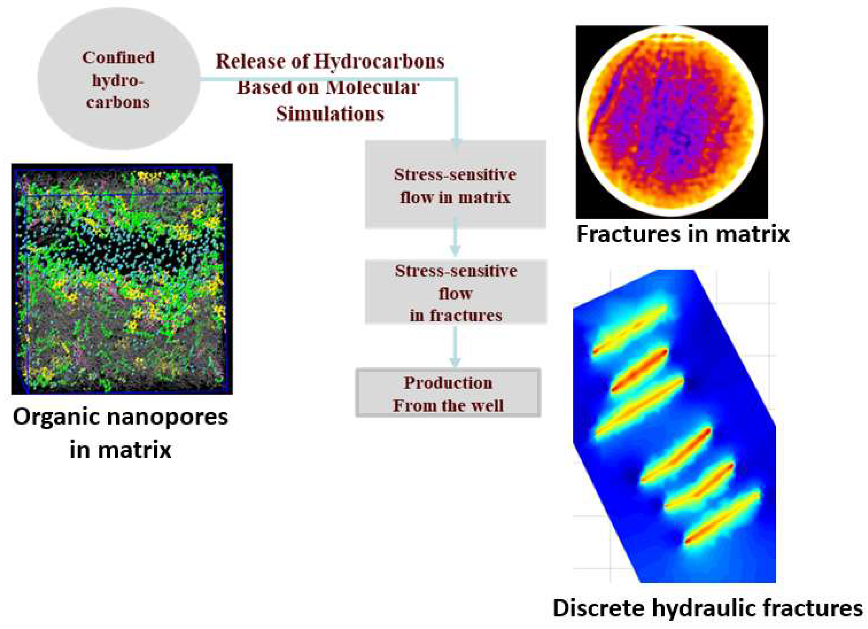
The final stage of development of the modeling effort involves the integration of this refined wellbore/fractures flow model with a reservoir flow simulator. The reservoir flow simulator NaSh is an in-house simulator employed in this study. The basic steps of creating the governing equations, the discretization of these equations, and numerical solution have been explained in Olorode et al. [12] in detail. NaSh is a sophisticated multi-scale compositional simulator coupled with geomechanics, and it offers a nuanced approach to model the dual porosity matrix in which hydraulic fractures are embedded. The dual-porosity matrix consists of organic (kerogen) pores and stress-sensitive natural fractures. The release of nano-confined hydrocarbons is based upon thermodynamic recovery calculations based on a molecular simulation [13,14]. NaSh is a compositional equation-of-state flow simulator in that it incorporates a comprehensive understanding of phase change, capillarity, stress dependency, and rock mechanics, all of which are considered for both the rock matrix and the fractures [15]. This capability enables a more accurate and detailed exploration of the complex interactions within unconventional reservoirs, particularly within the context of shale oil flow and production. In this case, a compositional flow simulator that considers the hydraulic fractures as discrete features embedded into the reservoir matrix has been used. Hence, the coupling allows interconnecting these fractures of the reservoir model with the fractures of the horizontal section of the wellbore.

The coupling creates a cohesive analytical framework that not only connects the understanding of reservoir and wellbore dynamics but also facilitates a more accurate and efficient analysis of the shale oil well performance The fluids volumes collected from the hydraulic fractures during the timestep Δt go through a flash calculation procedure, where their volumes are adjusted from the constant fracture pressure and temperature values to the standard conditions or some predetermined separator conditions. However, the resistances that are due to flow in the horizontal, the buildup, and the vertical sections of the wellbore were not included.

The reservoir simulation model NaSh traces the journey of hydrocarbon molecules from nanopores and fractures and in the matrix, and through the discrete hydraulic fractures to the wellbore. Figure 1 visualizes the workflow. Accordingly, reservoir fluids are allowed to migrate in the matrix from the nanopores to micro-cracks and to fractures. At the onset of flow, marked as time $t=0$, the pressure throughout the horizontal well equates to the reservoir pressure, setting the stage for hydrocarbon entry into the wellbore as the simulation progresses. Figure 2 shows the diagram explaining the numerical treatment of the flow in fractures and the estimation of the produced fluid volumes using reservoir flow simulator NaSh. After setting the parameters that control the behavior of the fractures, the volume of fluid delivered by these fractures is then used as the inner boundary condition for the reservoir simulator. The simulator computes the volumes of hydrocarbons and water produced by calculating the difference between the volumes existing within the total pore volume of the reservoir at time t₁ and that total volume at time t₀. This computed finite volume of hydrocarbons then represents the produced volumes. Using liquid–vapor equilibria (or flash) calculations, next, these volumes and their compositions are brought to the surface by being adjusted to the standard conditions; see Figure 2. The produced volumes needed are uniformly allocated across the designed fractures along the horizontal section.

2.3. Coupled Reservoir/Wellbore Flow Simulation Model, NaSh+

For this study, we coupled NaSh with the wellbore flow model described in Section 2.1 and Appendix A. The key difference in the NaSh+ simulation model is the connection of the reservoir/hydraulic fracture simulation data to the wellbore as the boundary condition shown in Figure 3. Once the wellbore receives the produced volume from the fractures, the wellbore flow simulator steps in to assess the liquid holdup and pressure gradient across each grid block within the horizontal section. The simulation process transfers pressure, in situ liquid, and gas (when applicable) from one grid block to the subsequent one, until the beginning of the buildup section is reached. This approach yields a revised average pressure for the horizontal section, denoted as $P_{avg}$, which then becomes the input for NaSh’s computations at the next timestep. This critical step ensures a seamless integration between the reservoir and wellbore flow simulations, facilitating a coherent flow of data and insights. The procedure is iteratively carried out, using NaSh+, including coupled matrix/wellbore flow, calculating the total hydrocarbon volume in the reservoir at $t=n+1$, and subtracting from the volume at $t=n$, to determine the hydrocarbon influx into the wellbore for the subsequent timestep. This sequential process of hydrocarbon migration through the wellbore, as modeled by the wellbore flow simulator, continues in this fashion until the final timestep is reached. Through this iterative and dynamic simulation approach, a comprehensive understanding of hydrocarbon flow from reservoir to surface is achieved, offering profound insight into the intricacies of well performance and the critical role of fracturing in enhancing hydrocarbon recovery.

Following the simulation of hydrocarbon transport through the horizontal section, the process extends to include the transfer of in situ liquid and gas volumes through the build-up and vertical sections of the well, ultimately reaching up to the wellhead. The volumes of liquid and gas are computed one last time to reflect the volumes at standard conditions. This crucial step ensures that the simulated production volumes are adjusted to account for changes in pressure and temperature as the hydrocarbons ascend towards the surface.

3. Field Study Using the Flow Simulation Model Nash

A single-well case study has been performed to compare the performance between NaSh and NaSh+ flow simulators independently using the primary production stage of a shale oil well. This well has previously been studied using NaSh in the absence of a wellbore flow simulator as explained previously. Hence, there was a significant volume of reservoir/fracture/well data available. The key quantities known for this study include the bottom hole pressure BHP, well geometry, production volumes of oil, liquid, and gas, wellhead pressure, and choke diameter. The geology, completion (including number of fracturing stage and fractures average length), and PVT laboratory data have been analyzed. The horizontal section of the well is 7000 ft long and consists of 440 uniformly distributed planar hydraulic fractures also known as the radiator model. The vertical length of the well is 8500 ft.

For this study, the measured fluid composition data were provided. This was necessary because NaSh is a compositional reservoir flow simulator. The given composition is taken as the initial fluid composition and used for developing a fluid model for the NaSh simulation study. PVTSim 5.0 was used to validate the oil model. The latter consists of five pseudo-components. Their equivalent concentrations and their critical properties and binary coefficients are predicted using a MATLAB R2020a optimization tool that involves matching lab-measured fluid properties such as oil and gas formation volume factors, oil viscosity and density, and gas viscosity (

Table 1. Thermodynamic properties of pseudo-components used in fluid modeling.

Pseudo-Component	Zi [%]	MW [g/mol]	Tc [K]	Pc [psi]	Acentric Factor	Vc [m3/mol]
CH4/N2	35.6	16.2	189.5	664.2	0.0086	9.884 × 10−5
C2-C3/CO2	17.0	35.7	337.1	665.5	0.1255	1.746 × 10−4
C4-C6	10.7	70.1	464.1	489.6	0.2413	3.098 × 10−4
C7-C9	11.8	107.6	557.0	425.8	0.5040	4.981 × 10−4
C10+	24.9	251.7	746.9	233.4	0.9424	1.322 × 10−3

). This approach ensures the utilization of precise and relevant fluid data for simulation purposes. By aligning these fluid properties with the laboratory data and those obtained from PVTSim 5.0, the figures validate the reservoir fluid model. Such benchmarking is crucial to confirm that the fluid characteristics in the wellbore match those used in NaSh model, thereby ensuring consistency in the simulation studies.

Note that, although NaSh is a compositional simulator, the wellbore simulator is non-compositional (i.e., black oil), such that the volume of oil and its physical properties are predicted using laboratory correlations. The volume of gas is predicted based on the solution gas–oil ratio trend of the black oil.

A comprehensive summary of all other essential parameters required for the simulation includes the well data, hydraulic fracturing data, multiphase flow data, geo-mechanical data, and model fluid data. However, some necessary data points were indeed not available. Consequently, specific assumptions have been made to facilitate the commencement of the simulation. Eighteen parameters were used as the calibration parameters of the production history-matching and optimization during a previous study. This study was completed under the guidance of the operating company for this well. The optimization process used a genetic algorithm and follows an evolution-based procedure that aligns the modeled output with the actual well performance data. The same approach is commonly used in other studies; see, for example Olorode et al. [9]. There are two categories of data for the optimization: the properties of the reservoir matrix and of the hydraulic fractures. Six out of 18 parameters are related to the fractures, and the rest of them belong to the reservoir matrix. These calibrated parameters highlighted in red in

Table 2. Hydraulic fracture calibration parameters.

	Parameter, Symbol	Unit	Range		Ref.
			Min	Max
	Half length, xf	m	80	120	112
	Height, h	m	22	33	27
Fracture	Initial Porosity, φm,ini	-	0.5	0.8	0.66
	Fracture initial permeability, kf,ini	mD	40	60	50
	Perm. Model Parameter, PmaxF	Psi	11,000	16,000	-
	Perm. Model Parameter, mexpF	-	0.22	0.33	-
	Fracture width	mm	-	-	7.6
	Initial Water Saturation, Sw	-	-	-	0.9
	Drainage area length	m	-	-	300

and

Table 3. Matrix calibration parameters.

	Parameter, Symbol	Unit	Range		Ref.
			Min	Max
Rock	Initial Porosity, φm,ini	-	0.09	0.15	0.12
	Pore volume Compressibility, cp	1/psi	2.4 × 10−5	3.6 × 10−5	3 × 10−5
	Rock initial permeability, km,ini	mD	400	600	500
	Perm. Model Parameter, Pmax	psi	22,300	33,500	N/A
	Perm. Model Parameter, mexp		0.09	0.14	N/A
	Initial Water Saturation, Swi	-	0.09	0.14	0.12
	Critical Gas Saturation, Sgc	-	0.08	0.12	N/A
	Critical Water Saturation, Swc	-	0.08	0.12	N/A
	Max. Gas Rel. Perm, krmG	-	0.8	1.0	N/A
	Max. Water Rel. Perm, krmW	-	0.8	1.0	N/A
	Gas Rel. Perm exponent, nGCorey	-	1.0	1.2	N/A
	Water Rel. Perm exponent, nWCorey	-	1.0	1.2	N/A

are a summary of all 18 calibration parameters. The calibrated parameters for the fracture consist of the fracture half length (x_f), fracture height (h), initial porosity (ϕ_m,ini), fracture initial permeability (k_f,ini), effective stress at zero permeability (P_maxF), and resistance of fracture to close under stress ($m_{expF}$). The calibrated parameters for the rock matrix include the initial porosity (ϕ_m,ini), pore volume compressibility (c_p), rock initial permeability (k_m,ini), effective stress at zero permeability (P_maxF), resistance of fracture to close under stress (m_exp), water saturation($S_w$), critical gas saturation ($S_{gc}$), critical water saturation ($S_{wc}$), maximum gas relative permeability ($k_{rmG}$), maximum water relative permeability ($k_{rmW}$), gas relative permeability exponent ($n_{G,Corey}$), and water relative permeability exponent ($n_{W,Corey}$). To initiate the optimization process in NaSh, a specific range of values was set for each calibration parameter. We assume a uniform water saturation profile at the initial condition. The computational algorithm then evaluates the cost associated with altering each parameter, by summing the percentage differences of each parameter. The simulation dedicated to calculating optimized parameters requires a minimum of 48 h to identify the most efficient combination of the optimized parameters. The optimized values from NaSh details the overall cost.

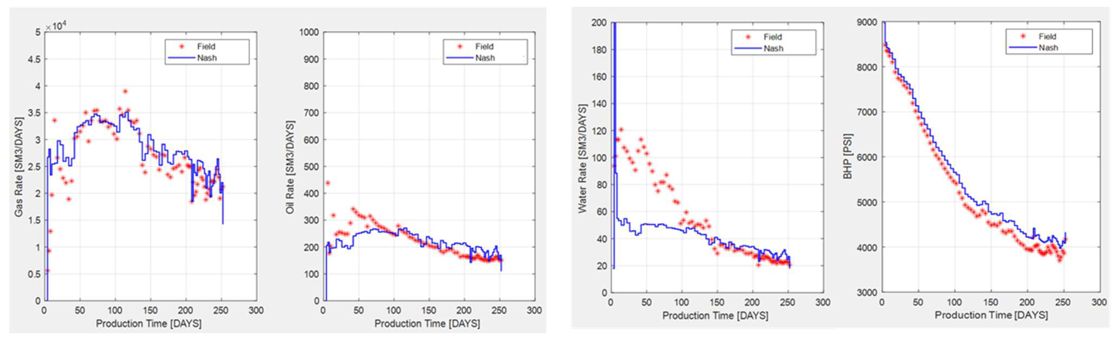
After all parameters are calibrated, the production history-matching results are shown in Figure 4. It can be observed that the results of gas rate, oil rate, water rate, BHP, WOR, and GOR closely match the field data, which proves a successful history-matching process. (Water–oil ratio and gas–oil ratio trends also match). The hydraulic flowback water can be attributed to the discrepancy during the early water production rates. These results underscore NaSh’s proficiency in executing an accurate history-matching process. Indeed, there exist discrepancies in the match shown in Figure 4 when compared to the real production data. But please remember that we will not use the match results for production forecasting. These discrepancies could be important for example in the case of reserve estimation. Here, our target is to maintain reservoir and fracture conditions that are optimum to perform a new investigation using forward simulation. This also means that slight changes in the optimized values should not lead to significant change in our observation and analysis.

The wellbore flow simulator processes the total production rates of oil, water, and gas computed using NaSh from the reservoir, where NaSh calculates the influx of hydrocarbons from the fractures into the wellbore by determining the change in the total hydrocarbon volume within the reservoir between two consecutive time points. For each timestep, NaSh determines the amount of oil, gas, and water distributed in the reservoir. The difference in volumes computed between the two consecutive timesteps is the produced volumes by the fractures, which are then input into the wellbore flow simulation by taking the total produced amounts and dividing by the number of fractures. During the simulation process, the pressure field is depleted, and the composition and phases of the fluids evolve, while the fluid properties are aligned with that change in pressure, ensuring both consistency and precision in the modeling. Then, these rates are evenly distributed across each fracture, sequentially transporting the fluid and pressure from the first segment from the toe of the well to the following one until they reach the surface. Most importantly, at the conclusion of each timestep, the average pressure of the horizontal segment P_avg is transferred to the NaSh model, where it becomes the new initial pressure for the reservoir simulation for the subsequent timestep. This process is repeated consistently, with each timestep’s average pressure of the horizontal section P_avg informing the initial pressure for the next. By accomplishing this interaction, NaSh is fully coupled with the wellbore flow simulator, with the inclusion of multi-phase flow interaction and fluid dynamics, and becomes the new sequentially coupled flow simulation model: NaSh+.

Ten parameters are selected to perform calibration of the model using NaSh+. Since the original version of NaSh has already proved to perform reasonably well on history-matching, the goal of the following analysis will reduce the calculation time by picking a smaller number of optimized parameters. After performing the optimization using NaSh+, the value of each parameter is compared with the case of NaSh when wellbore flow simulator was not coupled. The values for each optimized parameter are shown in

Table 4. Values of the 10 selected calibration parameters.

Case	xf	h	frac-perm	rock-poro	rock-perm	krmW	krmo	Sw	Soc	Swc
Fully-coupled	82.5	24.4	0.055	0.10	0.0005	0.96	0.84	0.11	0.10	0.098
Before coupling	111.8	22.4	0.05	0.13	0.0005	0.81	0.92	0.10	0.11	0.091

, in the sequence that they were inputted in the MATLAB script.

4. Validation of the Sequentially Coupled Reservoir/Wellbore Flow Simulation Model: Nash+

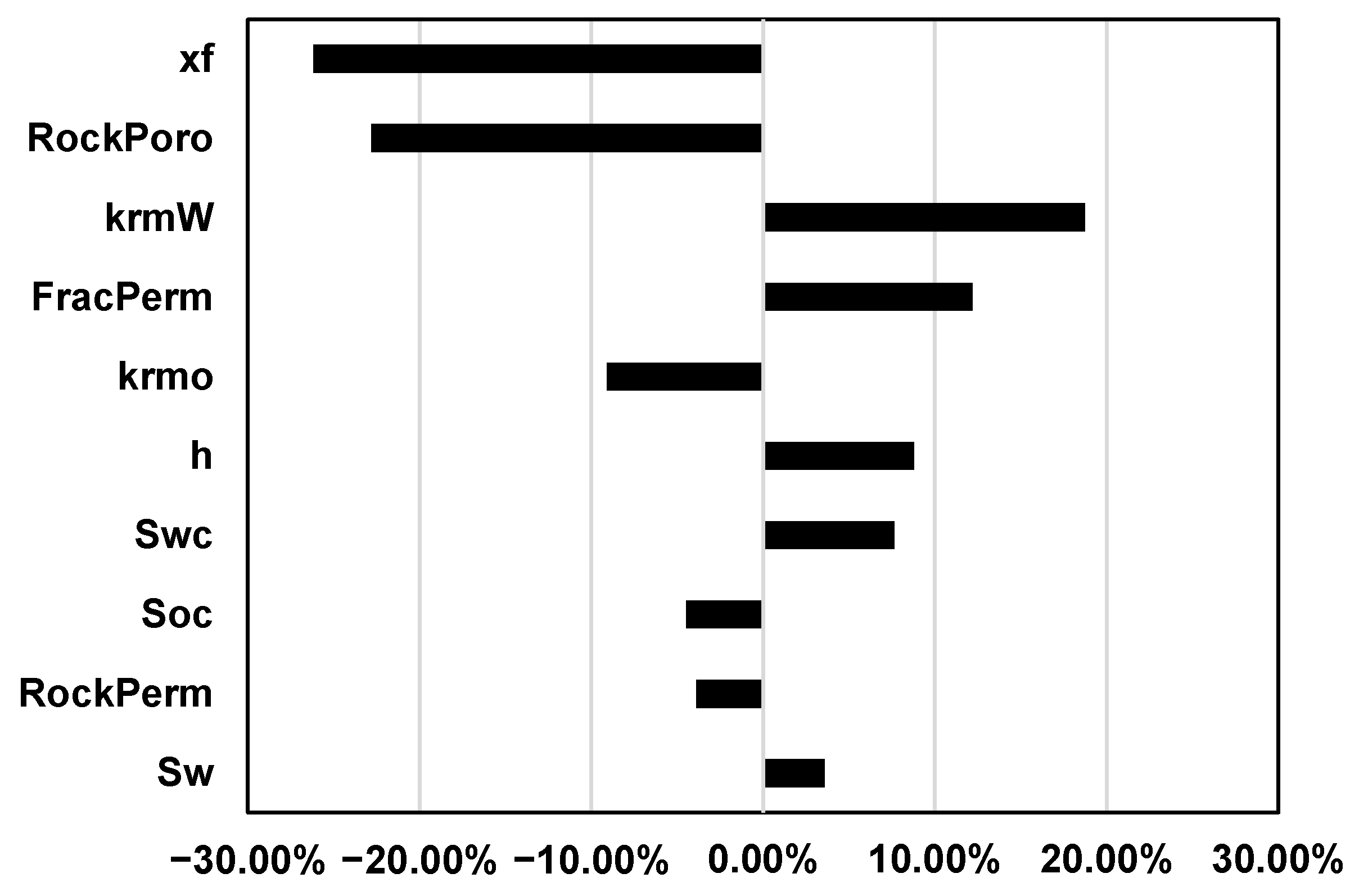
The percentage difference for the optimized values after sequentially coupling with NaSh+ is plotted in Figure 5, as a tornado diagram. In Figure 6 it is observed that NaSh+ predicts a 26% shorter fracture half length, which is a nearly 60 m shorter fracture. In addition, 23% less matrix porosity is predicted using NaSh. These indicate that wellbore flow is creating additional resistances which, in turn, is balanced by a reduction in the fracture length and porosity. Interestingly, it is also observed that the water and oil flow to the wellbore is being adjusted in the case of NaSh+ by increasing the water mobility by 19% and decreasing the oil mobility by 9%. This could be a potential impact of liquid holdup the wellbore experiences.

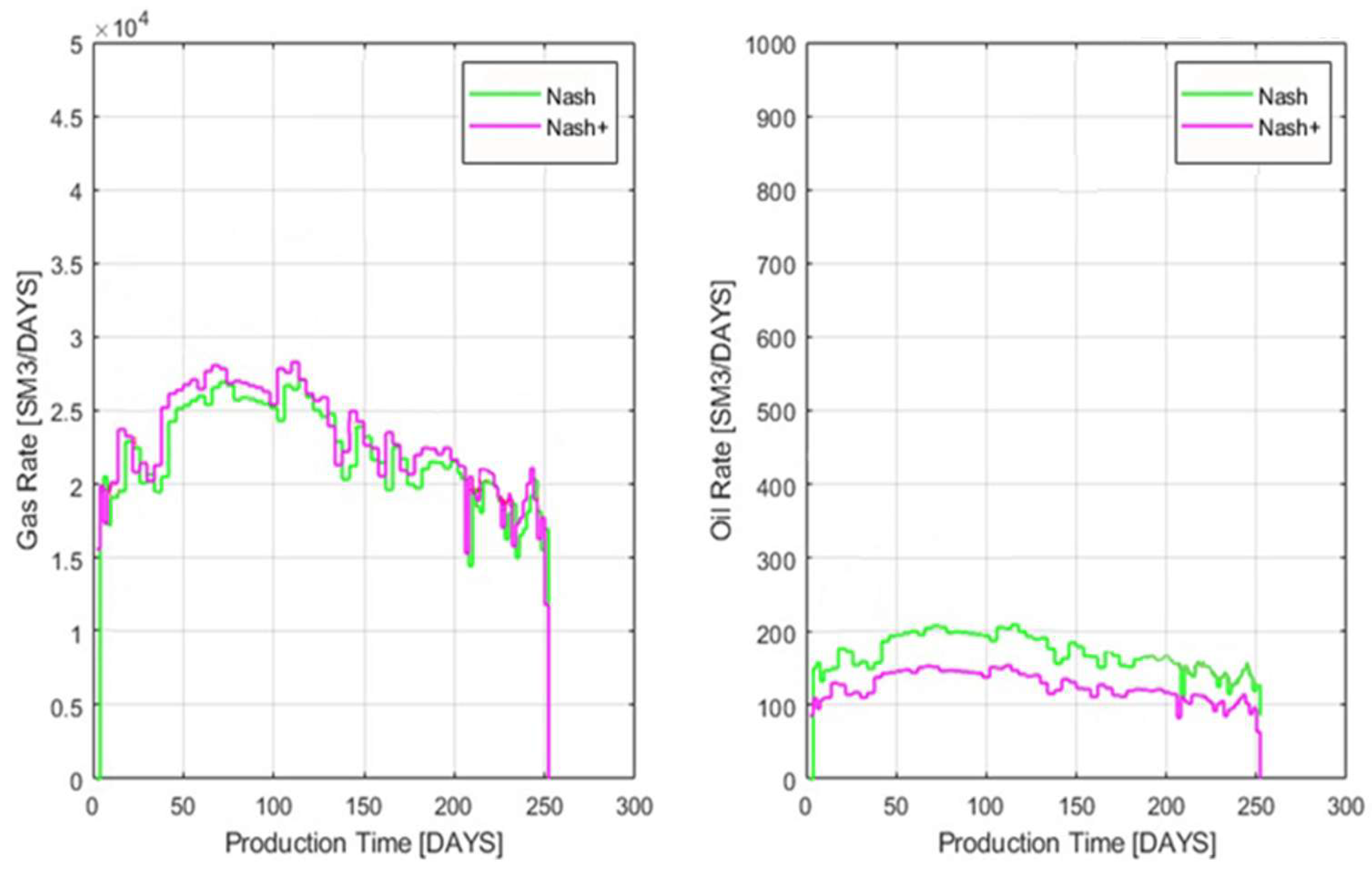
Upon employing the 10 optimized parameters, forward simulation runs were conducted for both the original NaSh and the fully-coupled NaSh+. Figure 6 illustrates the variations among field data, NaSh, and NaSh+ for both gas and oil production rates. The observed discrepancy between the green (NaSh) and magenta (NaSh+) lines highlights the influence of wellbore flow resistances, which are considered only after coupling with the wellbore flow simulator. This result aligns with expectations, as the inclusion of wellbore resistances and multi-phase flow interactions naturally tends to reduce production rates.

To validate the fully coupled simulator, NaSh+, a numerical approach is adopted where the lengths of both the horizontal and vertical sections of the shale oil well were progressively shortened. This strategy was employed to analyze the impact the varying degree of wellbore flow resistance has on the production rates of oil and gas at the surface. Based on this approach, when the total length of the well approaches to zero, the oil and gas production rates should be closer to the values obtained using NaSh, i.e., the simulations without the wellbore flow resistance. The cases considered are listed in

Table 5. Case studies on wellbore length using the sequentially coupled simulator NaSh+.

Case 1	Case 2	Case 3
10% Original Horizontal Length + Original Vertical Length	50% Original Horizontal Length + 50% Original Vertical Length	10% Original Horizontal Length + 10% Original Vertical Length

.

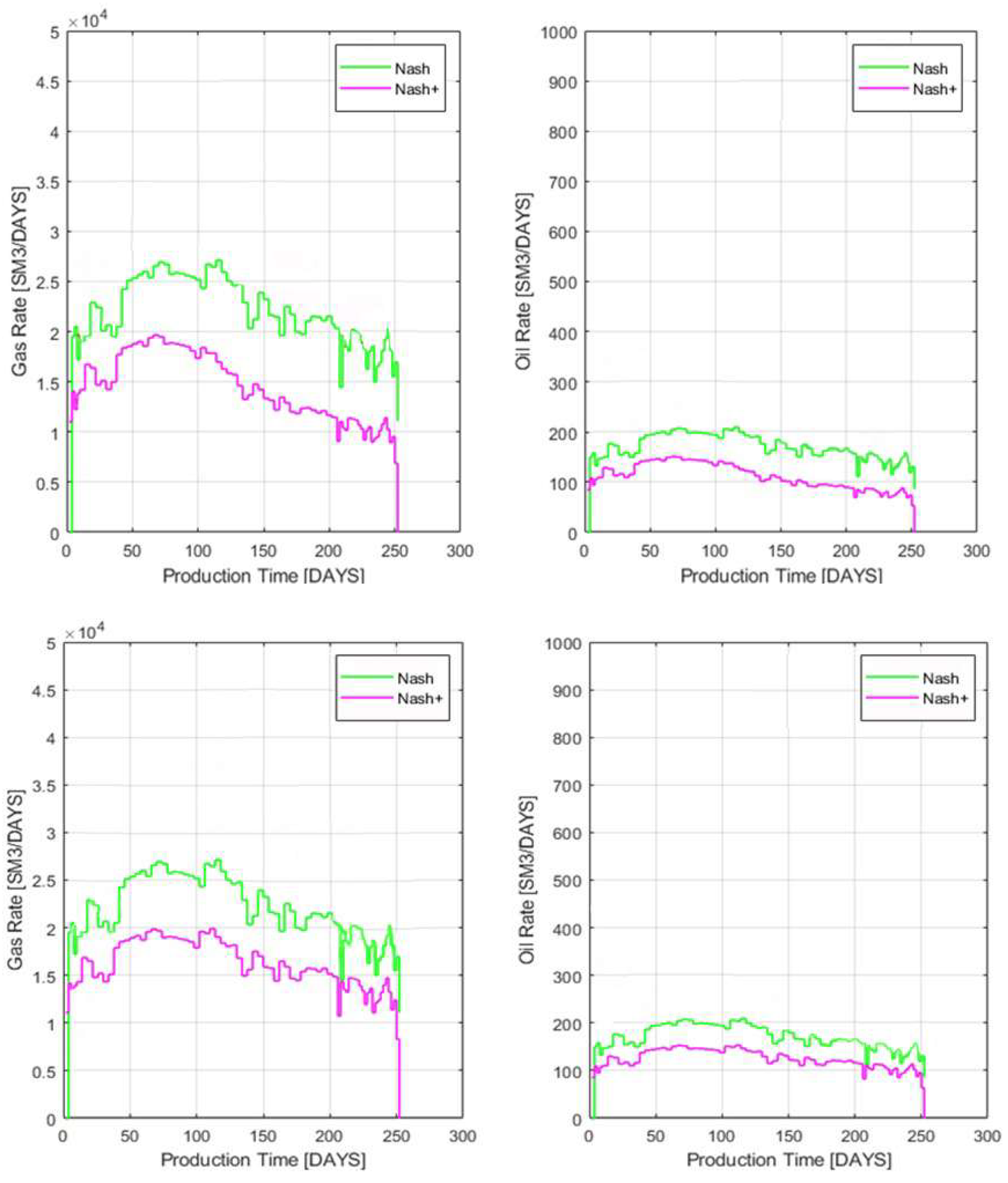
Figure 7 (top) demonstrates the production rates of gas and oil when the length of the horizontal section has been reduced to 10% of the original length from 7000 ft to 700 ft, where the rest of the wellbore remains the same length of the original case. It can be observed from the plot that changing the horizontal length of the well does not have a significant impact on the predicted production rates of gas and oil at the surface, indicating that the wellbore resistances in the horizontal section do not play a significant role during production.

In Case 2, the well’s vertical and horizontal lengths are reduced to 50% of their original values. The original vertical length of the well is 8500 ft; hence, taking half of this length results in a new vertical section measuring 4250 ft. Correspondingly, the horizontal section is reduced to 3500 ft. Given that the impact of the horizontal length on the production rates has been established as minimal, this case primarily concentrates on the effects of reducing the vertical section. Figure 7 (middle) shows oil and gas production rates for Case 2. Compared to the original case depicted in Figure 8, the production rates for both oil and gas in this adjusted case using NaSh+ are more closely aligned with the NaSh results, represented by the green line. With the reduced measured depth, the fluid now travels through shorter distances. This reduction in distance is expected to decrease the resistances caused by the wellbore flow; these resistances are a result of the reduced interaction between the fluid and fluid and the fluid and wall. As a result of the decreased resistances, there is a corresponding increase in the production rates of both gas and oil. This enhanced production efficiency is represented in the plot by the magenta line. This scenario underscores the critical role of wellbore dynamics in hydrocarbon extraction. By manipulating variables such as the measured depth, significant improvements in efficiency can be achieved numerically.

Figure 7 (bottom) presents the gas and oil production rates for this scenario, where the magenta lines indicate the NaSh results, and the green lines represent outcomes incorporating wellbore flow using NaSh+ with the reduced well dimensions. From the gas production rates on the left side of the plot, it is evident that decreasing the wellbore vertical length leads to NaSh+ predicted gas production rates that closely align with the NaSh results. This suggests a strong sensitivity of gas production to the vertical wellbore length, due to significantly decreased resistance encountered during the flow. In contrast, the right side of the plot, which shows oil production rates, reveals a less significant impact from shortening the wellbore length. This indicates that oil production is less influenced by the vertical length compared to gas production. The gravitational pressure gradient significantly influences the dynamics of the flow, particularly in the vertical sections of the well. This gradient arises due to the density differences among the fluid phases, namely, gas, oil, and water. As these fluids flow through the vertical sections of the well, gravity causes the denser fluids to segregate towards the bottom, while lighter fluids rise to the top. This stratification affects the fluid dynamics by altering the pressure conditions along the wellbore. Shortening the length of the vertical section leads to a lower gravitational pressure drop, which boosts the gas production rates at the surface.

The different responses with the modifications of length of the wellbore for gas and oil highlight the distinct fluid dynamics and resistance factors that each phase encounters during production. This case shows the importance of considering wellbore flow, particularly in gas-dominated systems, to optimize production strategies and well design.

5. Field Study Using Sequentially Coupled Reservoir/Wellbore Flow Simulation Model: Nash+

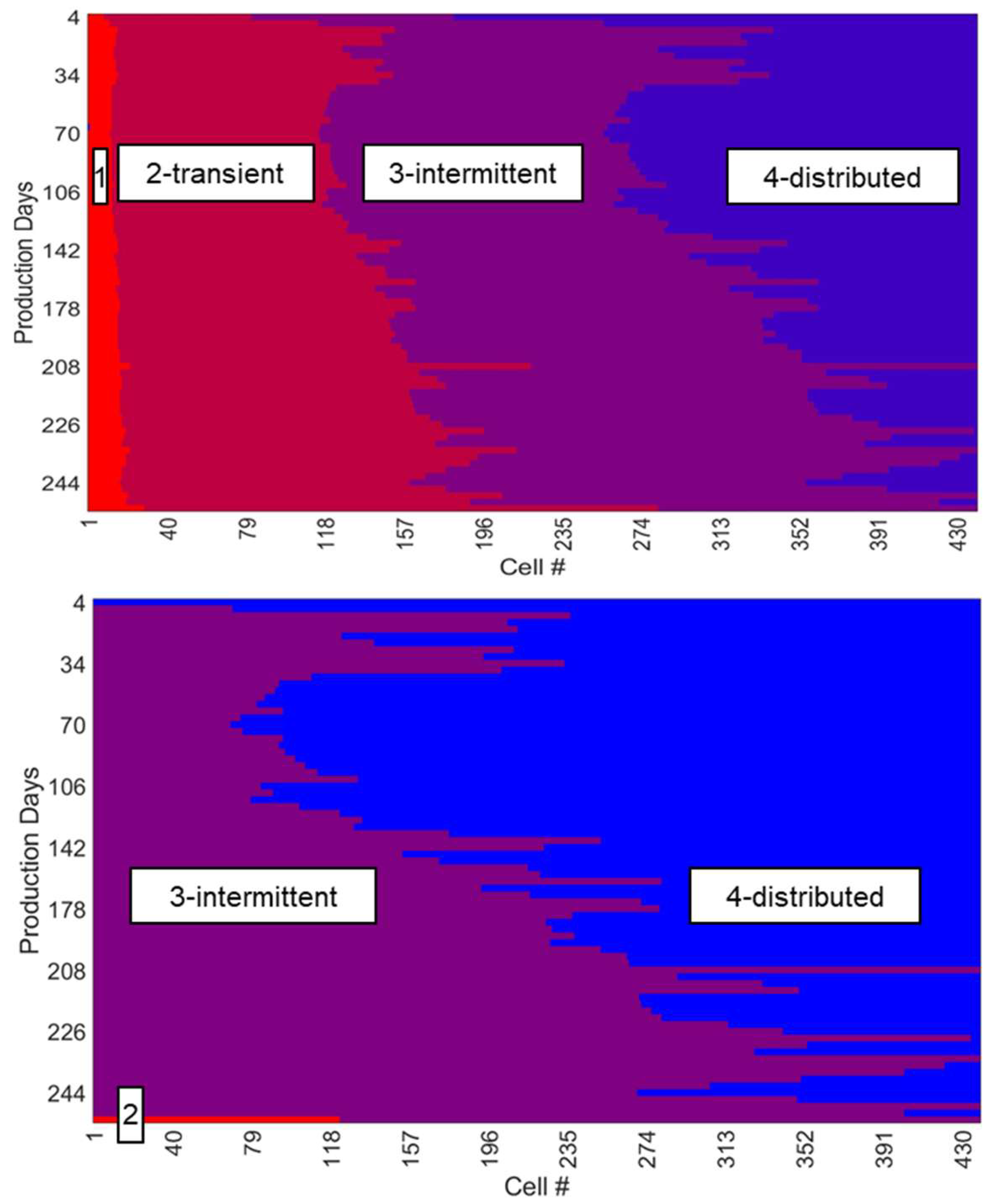
During the simulation, the flow dynamics along the horizontal well segment exhibit a distinct progression of flow regimes, influenced primarily by variations in liquid flow rates and inputs from the hydraulic fractures. A heatmap is generated using NaSh+ data to visualize how the flow regimes in the horizontal section change throughout the 250-day production and is shown in the top figure of Figure 8. The heatmap categorizes flow regimes into five distinct values: 1, segregated flow; 2, transient flow; 3, intermittent flow; 4, distributed flow; and finally, 5, other types of flow regimes. These flow regimes are selected based on the criteria listed in the Appendix A. Cell #1 represents the heel of the horizontal section, while cell #440 denotes the toe of the well. An analysis of the heatmap reveals the co-existence of multiple flow regimes (segregated, transient, intermittent, and distributed flows) throughout the production cycle. Notably, intermittent and transient flows are more prevalent in the middle of the horizontal section compared to the other regimes. Segregated flow is observed only in 6% of the lateral length, located close to the heel of the horizontal section, indicating its limited occurrence. Given that these horizontal wells have pressure gauges positioned close to the hell, the measurements should have added uncertainties in measurement error due to the flow of the segregated phases. Initially, distributed flow predominates near the toe, marking its significant role in early production stages. However, its dominance wanes after 140 days of production, with some periods where distributed flow is entirely absent.

On the fourth day of production, distributed flow emerges as the predominant flow regime, covering nearly two thirds of the length from the toe of the horizontal section. During this phase, the velocities of the liquid and gas phases are relatively similar, suggesting that while slippage may occur, it is likely minimal. Two days later, on the sixth day of the production, the flow regimes shift significantly. The once-dominant distributed flow recedes, making way for intermittent flow characterized by the formation of larger gas pockets at the top of the liquid layer. This transition marks a notable change in the wellbore’s flow dynamics, with intermittent flow increasingly taking precedence along the lateral extent of the well. As production progresses, intermittent flow begins to dominate, laying the groundwork for transient flow regimes marked by even larger gas pockets. This evolution points to a gradual but steady shift towards flow regimes characterized by more pronounced phase separation and dynamics. Over time, this progression continues until the flow stabilizes into a segregated flow pattern. In this final state, liquid and gas segregate into distinct layers, with the gas layer moving at higher velocities above the liquid, which travels more slowly at the bottom of the wellbore. By the last day of production, it can be observed that distributed flow rarely takes place in the horizontal section, indicating much more gas production during this stage of production, traveling at a higher velocity in the upper layer of the liquid. This sequential transition of flow regimes from segregated to distributed flow across the horizontal wellbore highlights the complex interplay between fracture injections and flow dynamics, underscoring the importance of considering these variations for the accurate simulation and optimization of well performance. The incorporation of hydraulic fractures in the horizontal section of the well facilitates a distinctive transition in flow patterns during production, which is markedly different from the pipe flow scenario, where flow regimes were observed to remain consistent throughout the wellbore. In contrast, the presence of hydraulic fractures introduces dynamic alterations in flow behavior, emphasizing the significant impact these fractures have on the fluid dynamics within the wellbore. This complexity introduced by hydraulic fractures allows for a more nuanced observation of how flow regimes evolve over time and under varying production conditions, highlighting the critical role of fractures in shaping the flow characteristics and enhancing the productivity of horizontal wells.

6. Impact of Stress-Dependent Fracture Permeability on Production Performance

The ability to predict changes in rock permeability under varying stress conditions is fundamental to advancing our understanding of subsurface fluid dynamics, which is critical for hydrocarbon recovery. Variations in stress can significantly alter the permeability of rock formations, impacting everything from the efficiency of hydrocarbon extraction to the stability of underground constructions. This complex interplay has been the focus of numerous studies aiming to delineate the underlying mechanisms. The variation of rock permeability as a function of stress has been investigated by various authors; see, for example, refs. [16,17]. Here, the mechanistic model that has been introduced by Gangi will be used. He developed his model on the permeability variations in both whole and fractured porous rocks by combining theoretical frameworks with empirical observations. His approach involves two distinct models: one for whole rocks and another for fractured rocks. For the whole rock permeability model, he introduced a mathematical formula to describe how permeability changes with pressure due to these deformations. For the fractured rock permeability model, he introduced the “bed of nails” model, which conceptualizes the rough surfaces of fractures as asperities (like nails) that affect fluid flow through their geometric arrangement and deformation under stress.

$$k=k_0{\left[1-{\left({\displaystyle \frac{P_{conf}-\alpha P}{P_m}}\right)}^m\right]}^3$$

(1)

The above equation was derived by applying confining pressure to split core samples under stress. The equation presents the relationship between the fracture permeability and the applied effective stress $P_{conf}-\alpha P$. Gangi validated his theoretical curves with the experimental data collected by Nelson (1975) [18] on a sandstone. Gangi’s model has been used to predict permeability change for split core samples under confining pressure $P_{conf}$. The above relationship assumes a power-law variation corresponding to the distribution of the length of asperity.

Later, the application Equation (1) has been extended to rocks that have permeability dominated by the presence of micro-fractures and cracks [19,20]. Previous students in my group used Gangi’s equation to study the effect of stress on the permeability of shale samples in the laboratory and showed the applicability of this model as the shale permeability model during simulation studies; see, for example, ref. [12]. Kim et al. [21] extended the application of Gangi’s mechanistic permeability model to the hydraulic fracture permeability under fracture closure stress. In their approach, the permeability models for the matrix and the fracture appear as follows:

$$k_m=k_{m0}{\left[1-{\left({\displaystyle \frac{{\sigma }_{OB}-{\alpha }_{m}P}{P_{m,max}}}\right)}^m\right]}^3$$

(2)

$$k_f=k_{f0}{\left[1-{\left({\displaystyle \frac{{\sigma }_h-{\alpha }_f{P}_f}{P_{f,max}}}\right)}^{m_f}\right]}^3.$$

(3)

Hence, although Equations (2) and (3) are similar in structure, the values of Biot coefficient α and the model parameters$k_0$, $p_{max}$, and m could change significantly since the hydraulic fractures are propped open and have added resistance to close under stress. Notice that the definition of effective stress changes depending on where Gangi’s equation applies. For the matrix, it is the overburden stress (vertical stress) that controls the behavior of the microfractures and cracks, and, hence, the permeability, whereas for the hydraulic fracture, it is the minimum horizontal stress. Although these stresses could be assumed constant during production, the effective stress (the nominator in Equations (2) and (3)) increases due to depletion of the reservoir and significant decrease in fluid pressure in the matrix P and in the fracture P_f. Using laboratory data, Kim et al. [21] showed variability in these parameters using shale samples from different basins in the US.

This exploration of closure pressure variations within rock formations reveals corresponding shifts in permeability. Such insights are invaluable in comprehending the stress–permeability relationship, a key information in optimizing fracture processes. Understanding the impact of stress on fracture permeability is crucial in refining fracture design and treatment strategies, thus enhancing their effectiveness and efficiency.

This section includes NaSh+ simulations dedicated to conduct a sensitivity analysis of Gangi’s model parameters and their impact on the production rates of horizontal well with hydraulic fractures. By exploring how these parameters influence reservoir behavior, this analysis provides critical insights into the fractured well’s response to environmental changes.

6.1. Sensitivity Analysis of Gangi’s Model Parameters

Hydraulic fracture conductivity is a critical factor in the extraction of resources from subsurface formations, and its dynamic nature is primarily due to the evolving conditions within the fracture over time. It quantifies a propped fracture’s capacity to transmit the fluids produced by a well, assessed through metrics like proppant permeability and the average width of the propped fracture. Initially, the permeability of proppants can reach hundreds of Darcys without applied stress. However, once within the subsurface environment, this permeability significantly decreases due to factors such as applied stress, proppant embedment, and crushing, as well as the complexities introduced by the flow of multiple fluid phases. In this chapter, results of a sensitivity analysis on the dynamic permeability field under stress is presented using NaSh+. During forward simulations, the permeability field, including both the matrix permeability and the fracture permeability, is treated as a dynamic field, where permeability values for each grid block are computed as a function of stress using Equations (2) and (3). This numerical scheme more accurately reflects the real-world conditions of a rock formation. As mentioned earlier, 10 parameters were selected for evaluation following the sequential coupling of NaSh with the wellbore flow simulator. Among these parameters, the initial fracture permeability ($k_{f0}$) is a key quantity for the analysis. Originally, the optimized value for $k_{f0}$ was determined to be 0.055 Darcy (D), based on an initial estimate of 0.05 D in the input file. 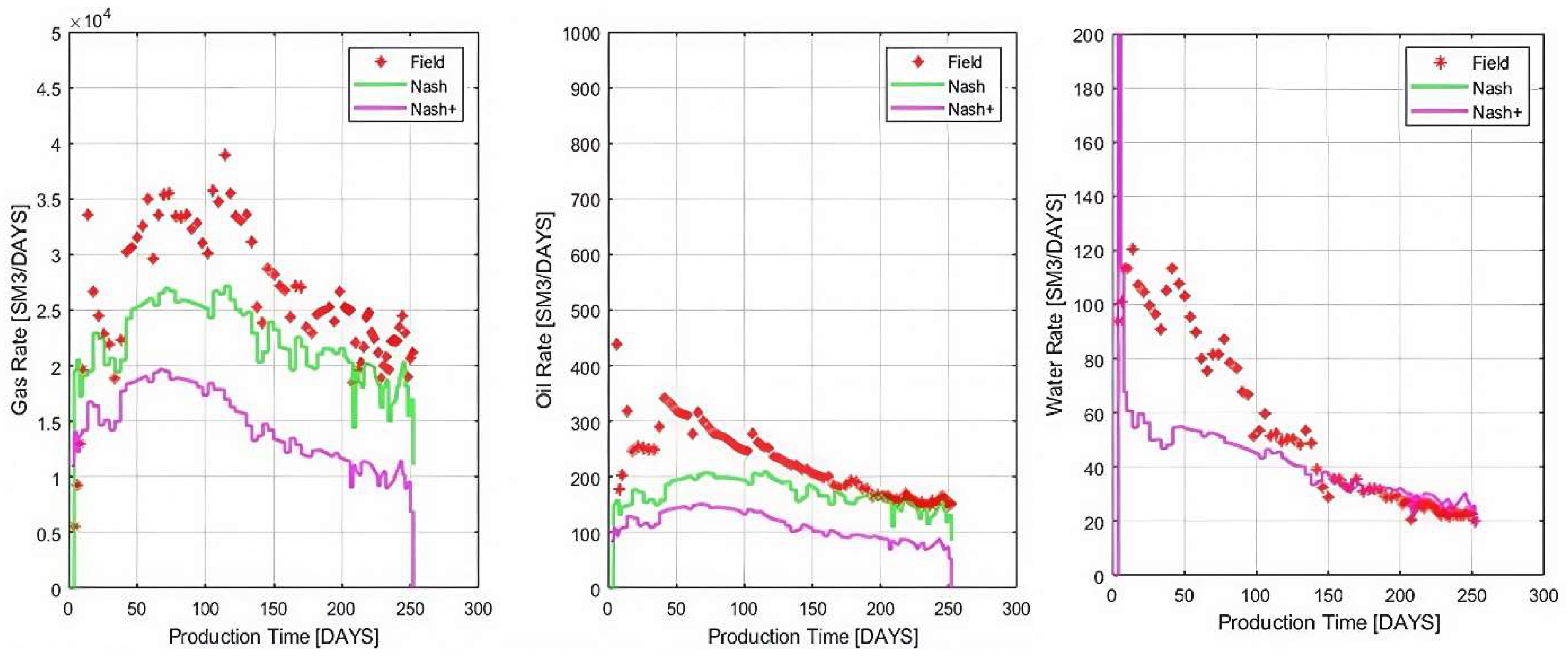Figure 9 illustrates a comparison of gas, oil, and water production rates among field data, results from NaSh, and results from NaSh+.

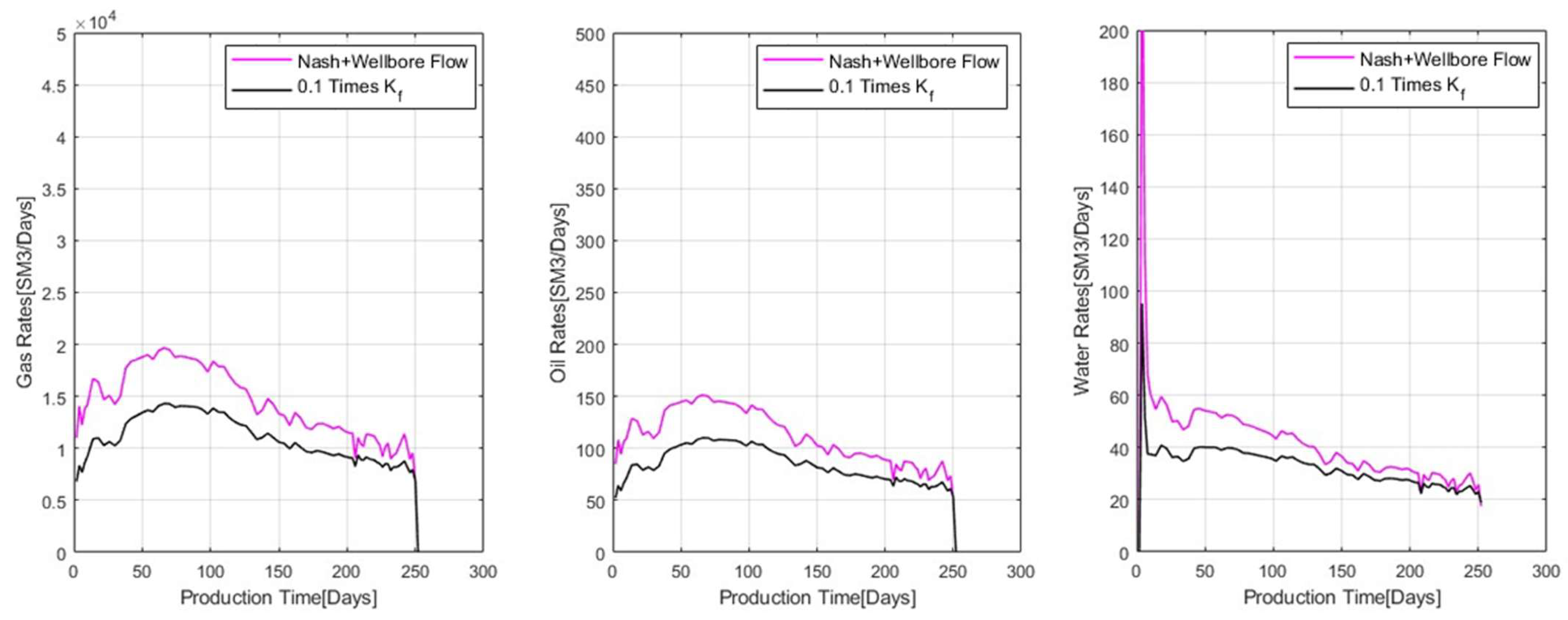
In subsequent sensitivity analysis plots, field data will be excluded, as the effectiveness and success of the history-matching process have already been established. Reducing the initial fracture permeability to one tenth of its original value yields interesting insights into production rates, as depicted in Figure 10. In this figure, the magenta line represents the original case, while the black line indicates the scenario $k_{f0}$ reduced to one tenth of its initial value. As anticipated, the reduction in fracture permeability has a noticeable impact on the production rates of oil, water, and gas at the surface. This is attributable to the fact that a lower initial fracture permeability impedes the extraction of hydrocarbons from the rock, leading to reduced production of gas, oil, and water. Additionally, the production of gas is more sensitive to the reduction in fracture permeability, which might be related to the pressure-sensitive oil properties. When permeability is reduced, the oil pressure in the fracture stays high; consequently, the release of dissolved gas and the formation of the mobile free gas phase are delayed. This leads to a reduction in the production of the gas rates. The difference in production rates between the two scenarios diminishes over a longer production period. In the original case, production rates decrease more rapidly than in the new scenario with reduced fracture permeability. The new scenario demonstrates a more stable and steady production rate over time, indicating that while initial production is lower due to reduced permeability, the decline rate is lower, possibly leading to more sustained production in the long term.

Sensitivity analysis is also crucial for reservoir modeling and production planning, while understanding how changes in fracture permeability impact production rates over both short and long terms can help in designing more efficient extraction strategies and in predicting the lifecycle of the reservoir more accurately. The Biot coefficient (α) measures how much change caused by pore pressure will contribute to changing the effective stress in the porous rock. In fact, the coefficient values are different for the matrix and the fractures, but we do not have proper literature that discusses the difference. The value of α ranges between 0 and 1. If α has a value of 0, it indicates that changes in pore pressure have no impact on the effective stress, whereas α value of 1 implies that the effective stress is fully sensitive to changes in pore pressure. The actual value of α depends on the porosity, compressibility of matrix and fluid, and overall mechanical properties of the rock (Biot 1941) [22]. In the case of α for hydraulic fractures, there exist added complexities of the proppant’s mechanical strength, the proppants arrangement along the fracture, and their rotation and displacement under stress. The base value of the fracture’s Biot coefficient (${\alpha }_f$) is taken as 1.0. Two more values of ${\alpha }_f$ values have been selected to perform sensitivity analysis using forward simulation, which are 0.5 and 0.2. During these simulations, ${\alpha }_m$ for the matrix was not changed and was kept at its original value, i.e., ${\alpha }_m$ = 1.0. 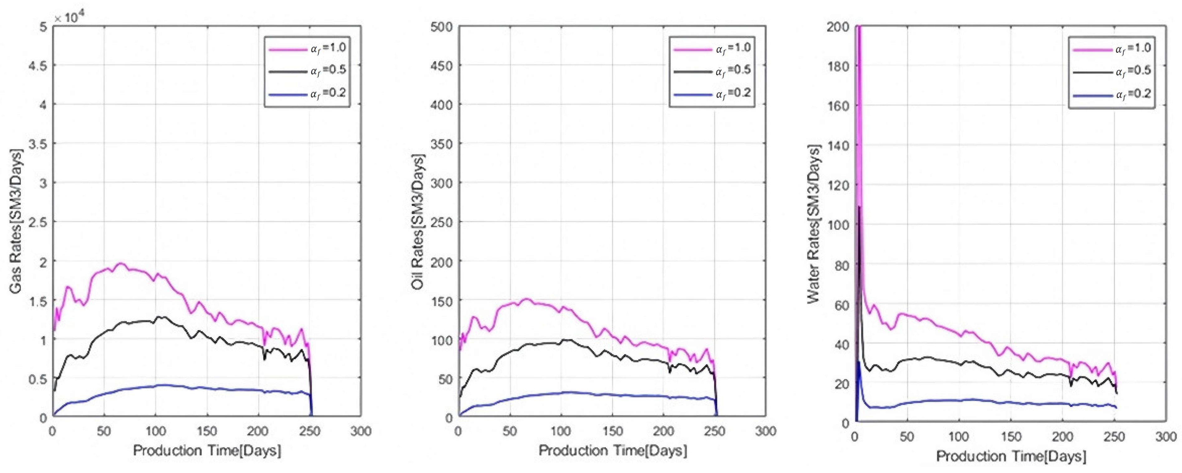Figure 11 illustrates the differences in the predicted production rates under three different values of ${\alpha }_f$ for the hydraulic fractures. The magenta line is the base case when ${\alpha }_f$ = 1.0, the blue line is when ${\alpha }_f$ = 0.2, and the black line is when ${\alpha }_f$ = 0.5. The trends clearly illustrate that higher values of fracture ${\alpha }_f$ are associated with increased production rates for gas, oil, and water, underscoring the significant role that ${\alpha }_f$ plays in determining the efficiency of hydrocarbon extraction. Equation (3) suggest that a larger $\alpha$ should enhance the fracture permeability ($k_f$) and, thereby, increase oil and gas production rates at the surface.

When examining the fracture permeability ($k_f$) profile depicted in Figure 12, for ${\alpha }_f=1.0$ (represented by the black line in the plot), a notable reduction in $k_f$ is observed along the fracture length. Conversely, for ${\alpha }_f=0.5$ (the red line in the plot), the decrease in $k_f$ is now less pronounced; yet, the overall $k_f$ remains lower compared to the case with ${\alpha }_f=1.0$. The scenario with ${\alpha }_f=0.2$ (the blue line), does not show a significant further drop in $k_f$ along the fracture, but the overall $k_f$ is lower than in the other cases. From these observations, it becomes clear that a higher ${\alpha }_f$ value is associated with greater $k_f$ within the fracture, which, in turn, facilitates increased oil and gas production into the wellbore. 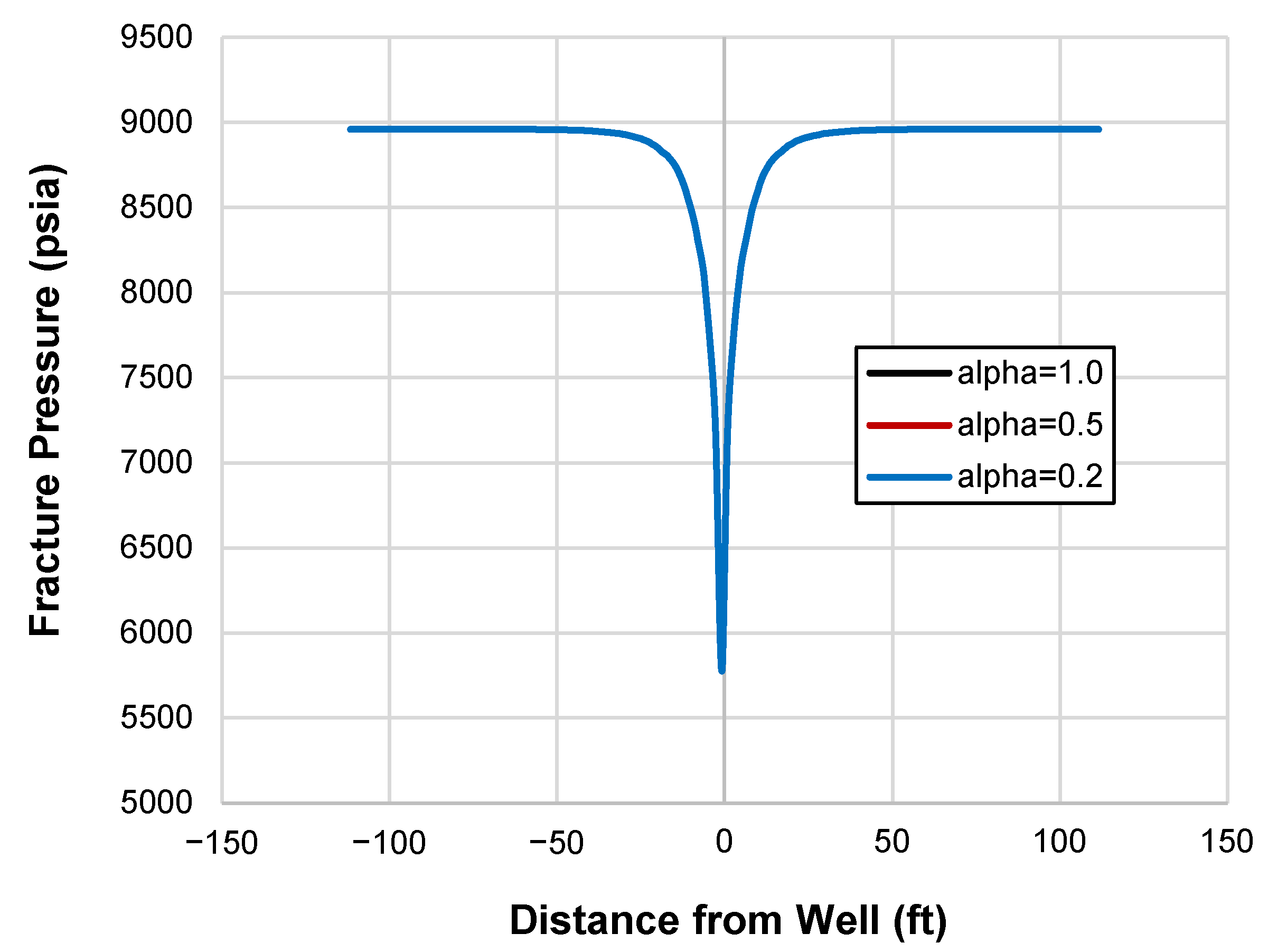The pressure profile along the fracture in Figure 13 shows that variations in the ${\alpha }_f$ do not alter the pressure distribution along the fractures. This finding highlights the nuanced role that ${\alpha }_f$ plays in influencing reservoir performance and production outcomes.

The sensitivity analysis conducted on the key parameters of Gangi’s model yields crucial insights for the optimization and design of hydraulic fracturing processes. Among these parameters, the initial fracture permeability k_f0 and Biot coefficient ${\alpha }_f$ emerge as critical parameters, exerting a considerable influence on the production rates of a well. These parameters fundamentally dictate the ease with which fluids can traverse the fracture network, thereby impacting overall production efficiency. Therefore, prioritizing the adjustment of initial fracture permeability and Biot coefficient could lead to more immediate and significant improvements in production rates.

6.2. Producing GOR Trends Under Static and Dynamic Fracture Permeability Fields

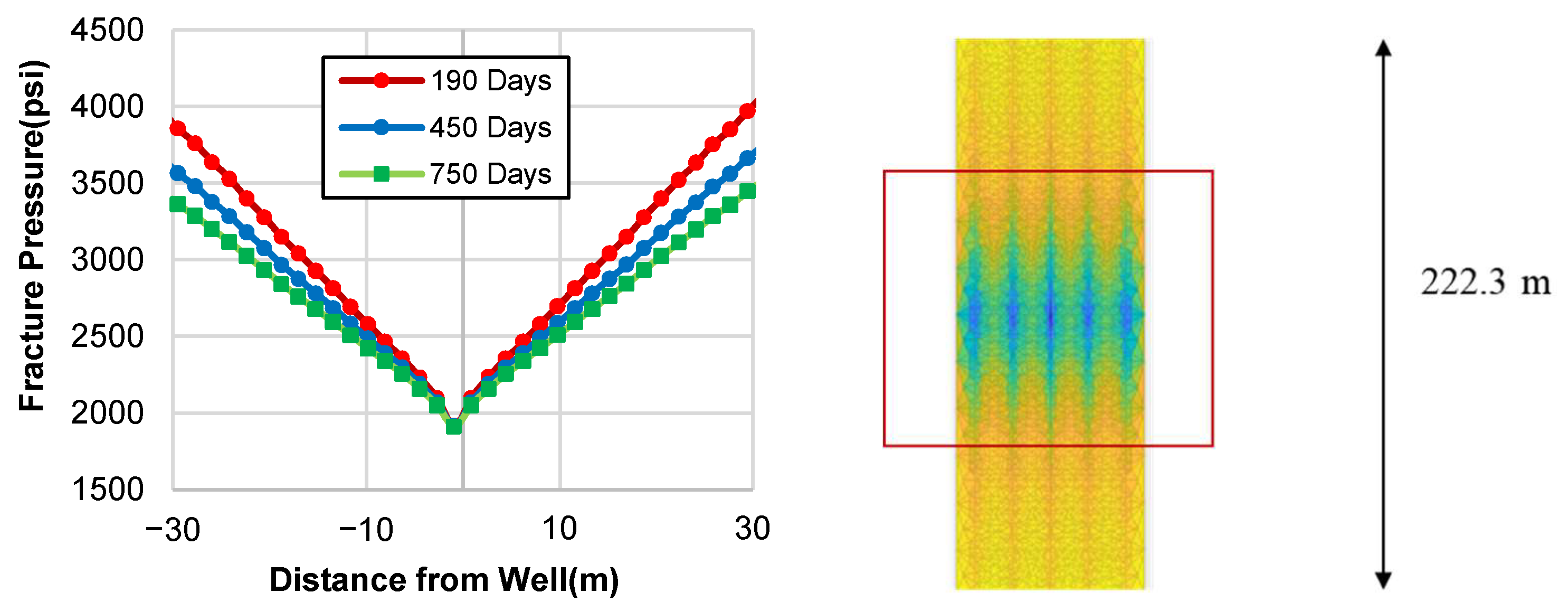
The simulation model used in this section considers running NaSh+ for the production of only one stage of fractures for the well. The model incorporates a detailed mesh structure in both the matrix and the fractures. As shown in Figure 14, notably, the mesh density increases progressively from the rock matrix towards the fractures. This design ensures a precise capture of the dynamic behaviors occurring within the fractures. Figure 14 presents the pressure field across the rock matrix and the hydraulic fractures. A key observation from this figure is that the pressure within the rock matrix after 750 days of production remains relatively constant up to the point of encountering hydraulic fractures (see large yellow outer regions). Beyond this point, a gradual decline in pressure is noticeable near the wellbore. This pressure distribution is indicative of the fluid dynamics and the influence of the fracture network on the overall flow within the reservoir.

Gaining insights into the producing gas–oil ratio, or, briefly, the GOR, during production is crucial, as the GOR plays an important role in presenting the characteristics of a reservoir and its production mechanism. It is a significant indicator that reflects the behavior and nature of the reservoir. A thorough understanding of the GOR assists in tailoring production strategies to maximize efficiency and output. It enables operators to adjust techniques to optimize extraction, based on the gas and oil interplay within the reservoir. Moreover, monitoring changes in the GOR over time serves as a diagnostic tool, signaling shifts in reservoir conditions. These changes can be attributed to various factors, such as reservoir depletion, the influx of water or gas, or alterations in reservoir pressure and temperature. Such variations provide an approach in reservoir management, potentially leading to strategic adjustments in field planning and decision-making processes.

To gain a deeper understanding of the production dynamics, two case studies were conducted using NaSh+ forward simulations. These cases focus on analyzing the impact of static versus dynamic hydraulic fracture permeability on surface production rates and the resulting GOR, with the details summarized in

Table 6. Case studies using NaSh+ forward simulations for analyzing producing GOR trends.

	Fracture Permeability	Matrix Permeability	Bottomhole Pressure, Pwf
Case 1	Static	Dynamic	1900 psi
Case 2	Dynamic	Dynamic	1900 psi

. Throughout these analyses, reservoir matrix permeability was maintained as dynamic in both scenarios, while the BHP was kept constant to isolate the effects of fracture permeability changes.

In Case 1, the fracture permeability is maintained as a constant throughout the production period, while the matrix permeability is allowed to vary dynamically. This case corresponds to the existing models in the literature, where the hydraulic fracture conductivity is often fixed to infinite conductivity. A fixed bottomhole flow pressure of 1900 psi is selected. The duration of this production simulation spans 750 days. This extended duration allows for a transition from the early stages of the well’s life to a mature and stable production phase in presence of multi-phase flow. The data, as depicted in Figure 15, reveal a consistent increase in the producing GOR over time. This trend indicates an escalating gas production relative to oil as the production process continues. The increase in gas production is primarily attributed to the fluid pressure dropping near the fractures falling below the bubble point, which triggers the evolution of gas from the oil phase.

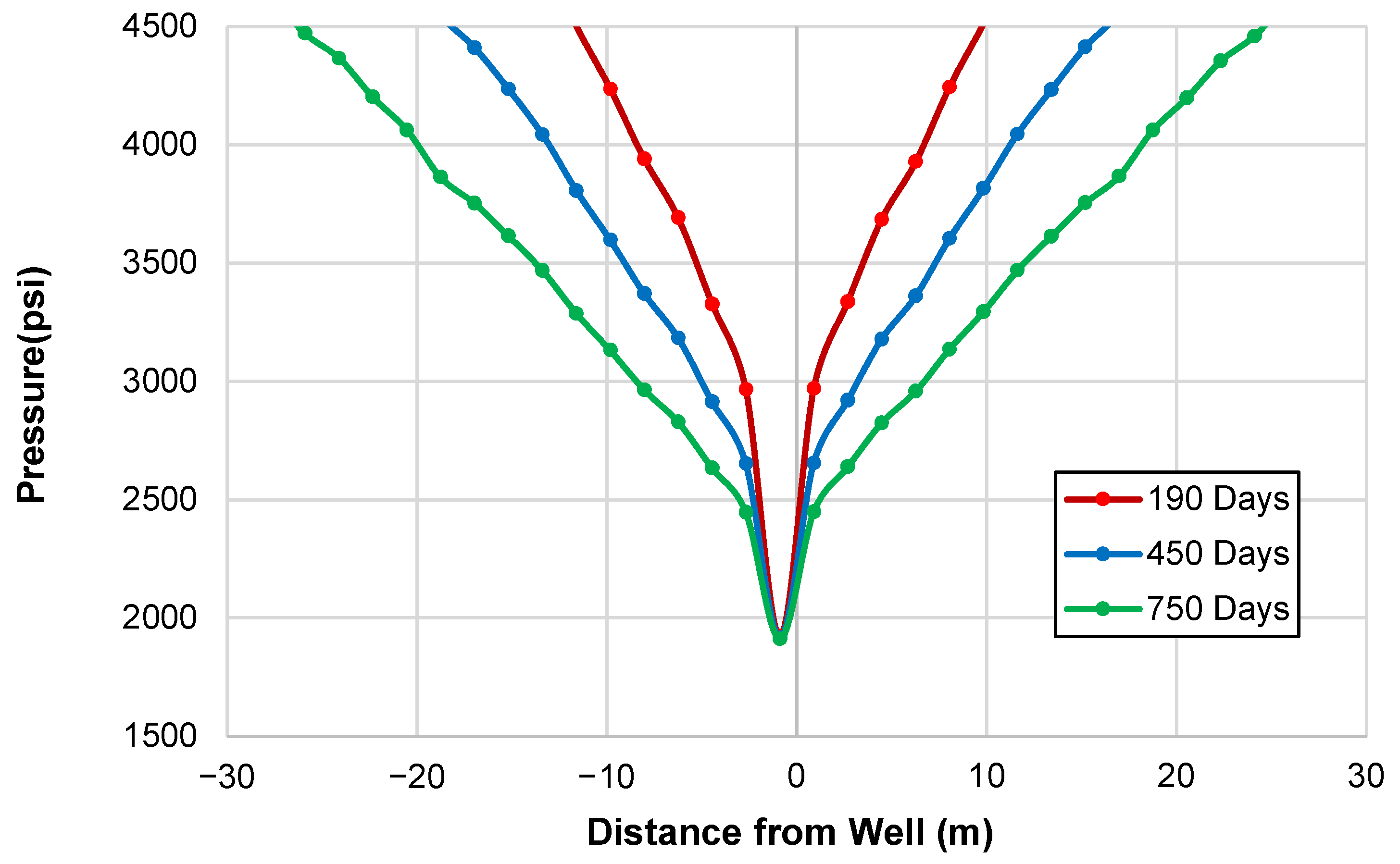
A more detailed analysis within the hydraulic fracture is presented in Figure 16 (Left) showcasing the fluid pressure profile along the fracture at different stages of production. This figure illustrates the pressure distribution at 190 days (red line), 450 days (blue line), and 750 days (green line) of production. The x-axis represents the near-wellbore region within the hydraulic fractures, correlating to the zoomed-in area displayed in Figure 16 (Right). The point where the distance from the well is zero corresponds to the center of the wellbore. The pressure profile indicates a gradual decrease in pressure from the tip of the fractures towards the center of the wellbore. As production progresses over days, the pressure in the fractures decreases, eventually reaching to the set BHP of 1900 psi. This pressure behavior is critical in understanding the fluid flow dynamics within the fracture system and provides insights into the evolving production characteristics of the well. The result of Case 1 highlights the dynamics of gas and oil production in presence of constant fracture permeability.

Case 2 is particularly interesting, because, unlike Case 1, the GOR remains relatively constant throughout the production, due to dynamic hydraulic fracture permeability. The BHP is still fixed at 1900 psi, and the production period is set to 750 days, consistent with Case 1. As depicted in Figure 17, the initial 250 days of production maintain a flat GOR profile, under dynamic fracture permeability. The stability in production is further evidenced by the GOR trends, where a notably flat and stable GOR is observed with 750 days of production, contrasting with the increasing trend noted earlier in Case 1.

To better understand the underlying mechanics of this behavior, Figure 18 offers a closer examination of the pressure profiles along the fracture, particularly in the near-wellbore region. The color-coded lines in the figure represent different production stages: 190 days (red), 450 days (blue), and 750 days (green). The observed pressure drop of Case 2 is different from that of Case 1, especially at the near-wellbore region. The pressure drop in the case of dynamic fracture permeability is notably more significant compared to static fracture permeability scenarios. During various stages of production, the pressure drop across the fractures exhibits a wide range, extending from 5100 psi to over 6600 psi. Moreover, the pressure drop trend near the wellbore region is particularly pronounced, where a sharp decline of more than 500 psi is recorded within just 3 m along the fractures. This steep gradient near the wellbore suggests that the dynamic adjustments in fracture permeability greatly influence the local fluid dynamics, leading to substantial localized pressure reductions. When comparing these observations to scenarios with static fracture permeability, it becomes evident that the dynamic permeability case leads to more variable and, generally, a higher pressure drop across the fracture wellbore interface during production. Unlike in the static case, where pressure drops tend to be more uniform and less pronounced, the dynamic case exhibits fluctuations that highlight the interplay between fracture permeability changes and fluid flow patterns.

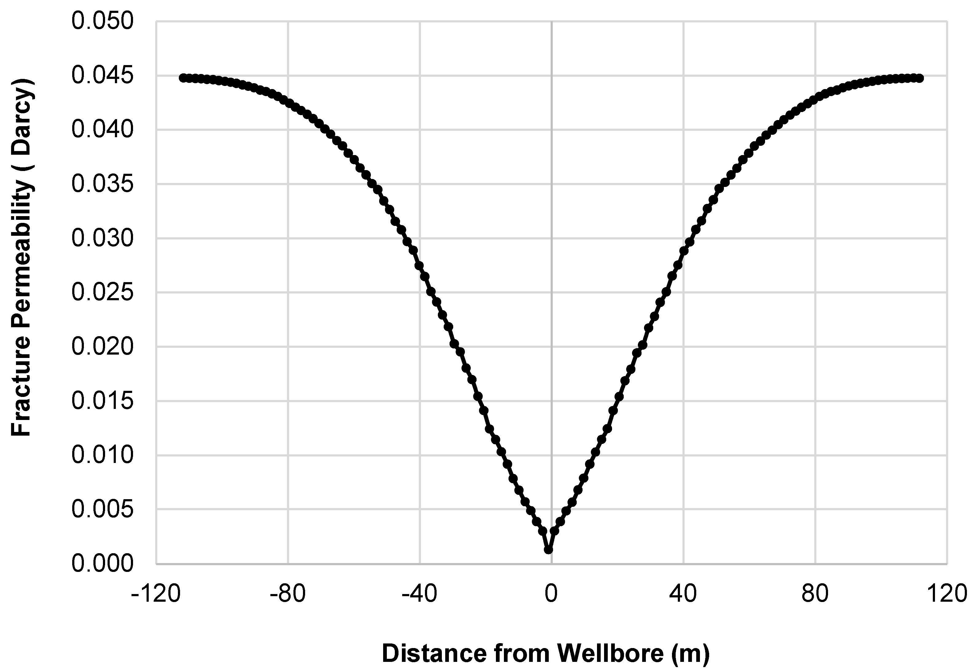
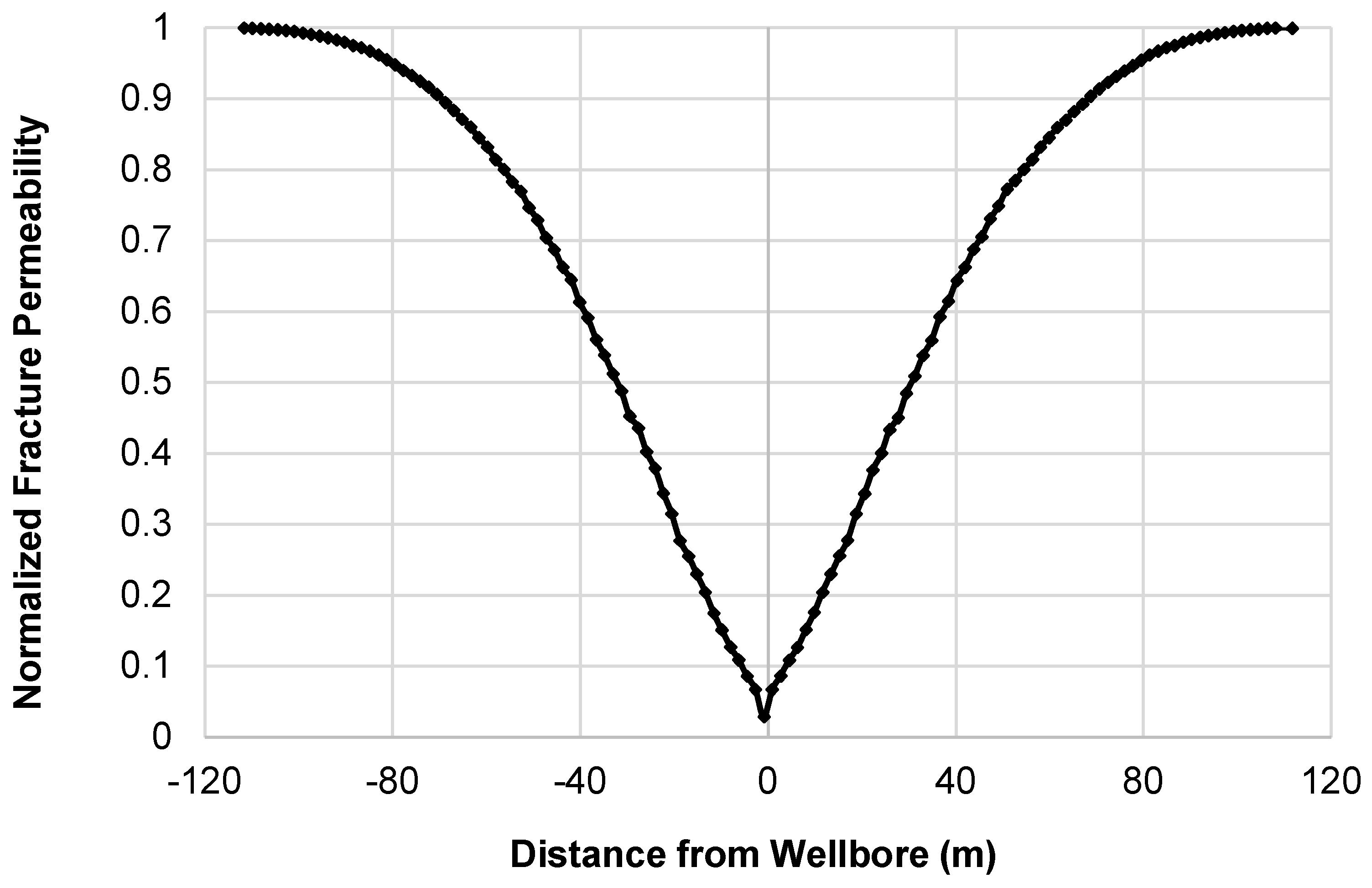
The next step is to investigate the cause of the pronounced pressure drop in Case 2 observed during the 750-day production period, particularly the pressure drops in regions close to the wellbore. This analysis is essential in understanding the dynamics of fluid flow within the fracture network, especially as it demonstrates changes in permeability over time versus the distance from the wellbore. Initially, at the far end, towards the tip of the fracture, the permeability is recorded at 0.045 D. Near the wellbore, particularly within 30 m, a gradual decrease in fracture permeability is noted. The most significant change occurs in the segment extending from 100 m to the center of the wellbore, where fracture permeability sharply declines, reaching a value as low as 0.0013 D near the wellbore. For a clearer representation of how dramatically fracture permeability varies within the fracture, the permeability at each point is normalized by dividing it by the initial fracture permeability noted at the far end. This normalized permeability, depicted in Figure 19, illustrates that approximately 60 m from the wellbore center, the permeability has reduced to 60% of its original value. Closer to the center, at the wellbore itself, it decreases to only 3% of the initial permeability. In other words, 97% of the fracture permeability is lost; see Figure 20. This significant reduction in fracture permeability along the fracture length highlights the presence of a choking effect on the wellbore. The term “choking effect” in this context refers to a substantial restriction in fluid flow caused by the drastic reduction in permeability. As the fractures near the wellbore become less permeable, their ability to efficiently transmit fluids is greatly diminished. This phenomenon has critical implications for production strategy, as it indicates a diminishing efficiency of the fractures closer to the wellbore over time as the fracture closure stress grows. Understanding this dynamic is essential for optimizing well performance. It suggests that adjustments in production techniques, such as well stimulation or alterations in production rates, might be necessary to control the stresses and mitigate the choking effect and sustain optimal fluid extraction rates.

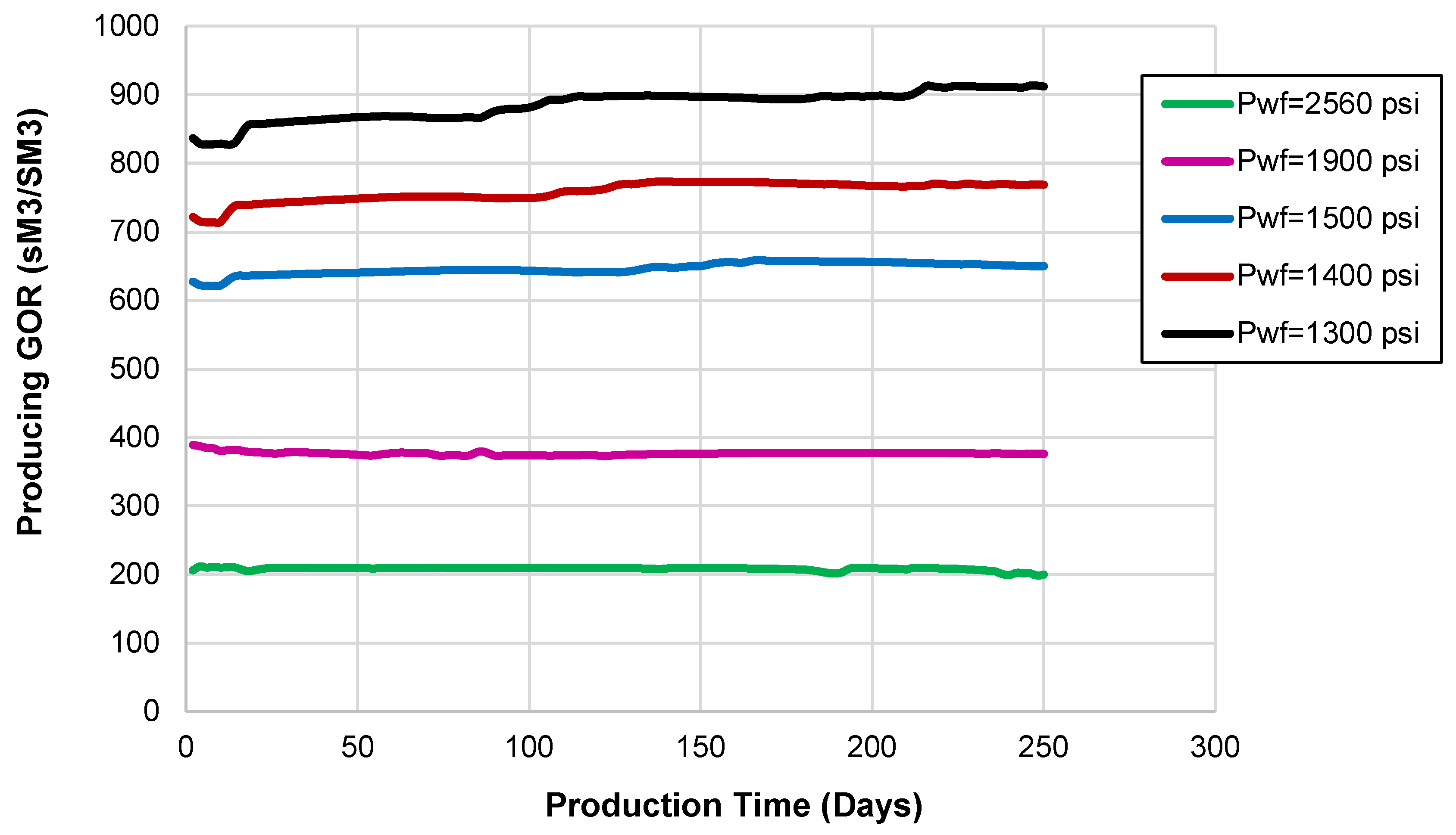
Having identified the choke effect of the fractures on the production, reviewing Figure 17, we notice that the choke effect could be tuned; hence, a flat GOR level could be controlled by simply controlling the BHP. If, for example, the operator of the well desires a producing GOR ratio of 500 SCF/STB, the BHP should be fixed between 1500 < P_wf < 1900 psi. This could be conducted, for example, using artificial lifting. Or, if the operator desires to minimize the producing gas–oil ratio, simply by mechanically choking the well at the wellhead, the BHP can be maintained at a high level such that P_b < P_wf. In essence, we optimize the production trends by controlling the choke effect of the hydraulic fractures. This discussion, however, precludes the extreme choke effect when fracture conductivity is severely reduced and when oil and gas rates are impaired significantly. In the latter case, the choke effect becomes a problem to mitigate. This can be achieved by reducing the BHP in small intervals using a surface choke management approach. Many shale wells in USA have already gone through a choke management plan, although the plan was originally implemented to control formation/fracture damage, not for the in-situ fracture choke effect.

7. Conclusions

The integration of reservoir and wellbore flow simulation models in this study advances our understanding of two-phase flow in multi-fractured horizontal wells, bridging the gap between conventional simulation results and real-world data. By incorporating the dynamics of two-phase fluid behavior and the impact of hydraulic fractures permeability, the enhanced model offers a nuanced and accurate representation of subsurface dynamics, which is crucial for refining well design and operational strategies. Insights from the shale oil well case study underscore the critical importance of coupling reservoir and wellbore flow simulators to avoid overestimating reservoir characteristics such as oil storage capacity and fluid accessibility. The findings suggest that prioritizing adjustments in the initial fracture permeability and Biot coefficient during simulation modeling can significantly improve production rates. Additionally, the study reveals that while static fracture permeability results in a smooth pressure drop, dynamic fracture permeability can lead to flat producing GOR and substantial pressure drops near the wellbore due to the “choke effect”, caused by a drastic reduction of 97% of the original fracture permeability at the center of the wellbore. These developments are important for optimizing resource recovery and enhancing the sustainability of production operations, emphasizing the need for comprehensive modeling tools that reflect the complexity of real-world oil and gas extraction scenarios. Operating companies observed the constant producing gas–oil ratio (flat GOR) trend with the shale oil wells. However, the literature has attributed the trend to several other factors [23,24,25].