Classical and Advanced Controllers for Ideal Halbach Magnetic Lead Screw for Ocean Wave Energy Applications ^†

Abstract

A magnetic lead screw (MLS) uses the magnetic field of permanent magnets to convert between linear and rotational motions while achieving a gearing action. This mechanism converts low-speed, high-force linear motion to high-speed, low-torque rotational motion. The MLS is ideal for wave energy applications, where the low-speed oscillatory motion of waves can be converted into usable electrical energy. It harnesses the high-force, low-speed linear motion of waves and converts it into rotational motion for generators, all while maintaining contact-free power transfer, reducing maintenance and machine size compared to linear machines. In this study, two controllers are proposed for an ideal Halbach magnetic lead screw: a proportional-resonant (PR) controller and an observer-based state feedback controller (O-SFC). The proportional-integral (PI) controller is also presented as a benchmark. These controllers are developed based on the linearized model of the ideal Halbach MLS and validated through simulation studies of its non-linear model. Results show that both the PR and O-SFC controllers significantly improve system performance compared to the PI controller, with the O-SFC providing superior performance over both the PR and PI controllers.

1. Introduction

After the oil crisis in the 1970s, there has been a growing global shift towards using renewable energy, driven by the need for both a sustainable and eco-friendly energy supply [1]. Among the main renewable energy options are wind, solar, and ocean-based power. The fact that oceans cover roughly $70\%$ of the Earth’s surface and hold around $97\%$ of its water makes ocean energy an intriguing area of study. This energy is generated through the interaction between the wind and the ocean surface, which causes pressure and friction, leading to the formation of waves. These waves, propelled by the wind, can continue moving long after the wind has ceased, gradually losing energy as they travel. The strength of a wave is directly linked to wind speed: faster winds produce larger waves and, thus, more energy. The global wave energy resources are estimated to be at least 1 TW, with an annual energy production capacity of about 2000 TWh. This type of generation is similar to the generation of electricity from nuclear or hydroelectric power [2]. This makes extracting energy from ocean wave energy an essential area of research. The point-absorbing type wave energy converter (WEC) stands out as one of the most promising technologies for commercial use. It has significant potential to generate high-power wave energy among existing types. This is due to the buoy’s ability to float on the wave’s surface and directly capture wave energy. Consequently, the buoy movement mirrors that of the waves, showing high force, slow speed, and reciprocal motion [3]. A report in [4] presented findings from a water tank test to evaluate the power performance of a heave-actuated point absorber WEC under varying conditions, emphasizing the influence of drivetrain stiffness and control strategies on electrical power capture. In [5], an impedance matching-based control design for wave energy converters is presented, addressing the gap between theoretical and practical implementation. Furthermore, it was concluded in [6] that the magnetic lead screw (MLS) results in higher output power for wave energy application compared to linear tubular generators.

There are a number of difficulties in turning wave energy into electrical power. Traditional wave energy converters often suffer from poor force density, large machine sizes, and high maintenance costs, according to [7,8]. Since the size of a linear electric generator is directly proportional to the forces it must interact with, the high-force, low-speed characteristic of wave motion helps explain the enormous size of these generators. Oscillating water columns, oscillating bodies, and overtopping devices are the main kinds of wave energy conversion systems [9]. Potential wave energy applications are studied in [10,11] when using an electromagnetic lead screw, in ref. [12] when using a reluctance MLS, and in [3] when using an MLS with reduced permanent magnets (PMs). Also, ref. [13] proposed a method for shaping the desired ideal helix for easier manufacturing, specifically for use in wave energy applications. 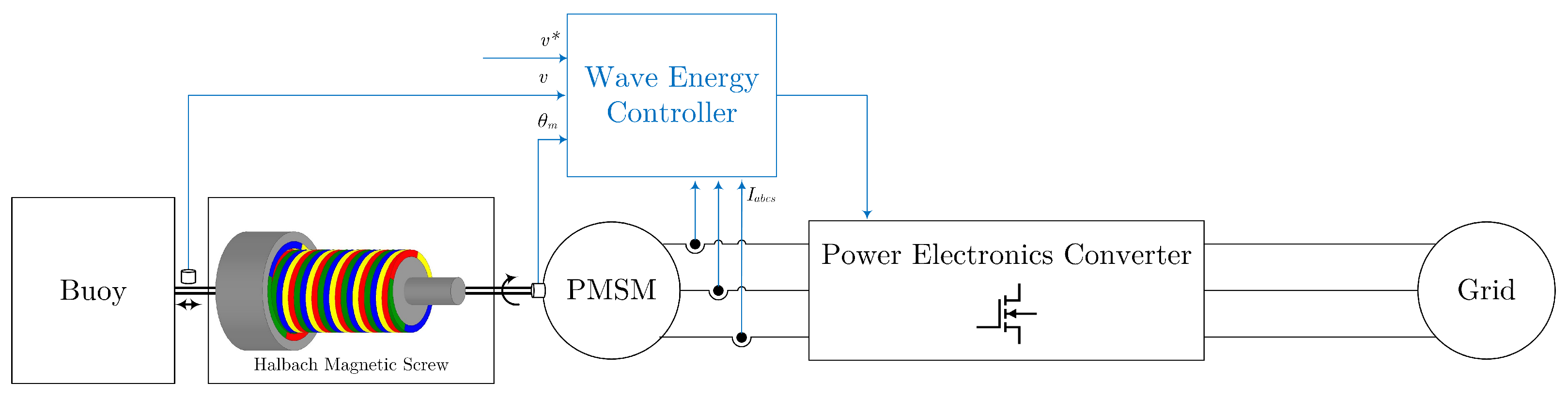Figure 1 illustrated the entire procedure of using a Halbach MLS to transform wave energy into electrical power and supply it to the grid. The buoy’s linear motion will be transformed into a rotational motion by the Halbach magnetic screw, which powers the permanent magnet synchronous generator (PMSM), which is linked to the electrical grid via a power electronics converter. The wave energy controller will be the special topic of this study.

Different topologies of MLS are presented in the literature, including ideal-helical [14,15,16], embedded magnets [7], discretized [17,18], field-modulated [19,20,21], reluctance-based [12,22], electromagnetic screw [10,23], Halbach MLS [24], and discrete Halbach MLS [25,26,27]. In [28,29], a thorough literature study was carried out on the various MLS topologies, MLS analytic techniques, modeling, control, and machine integration.

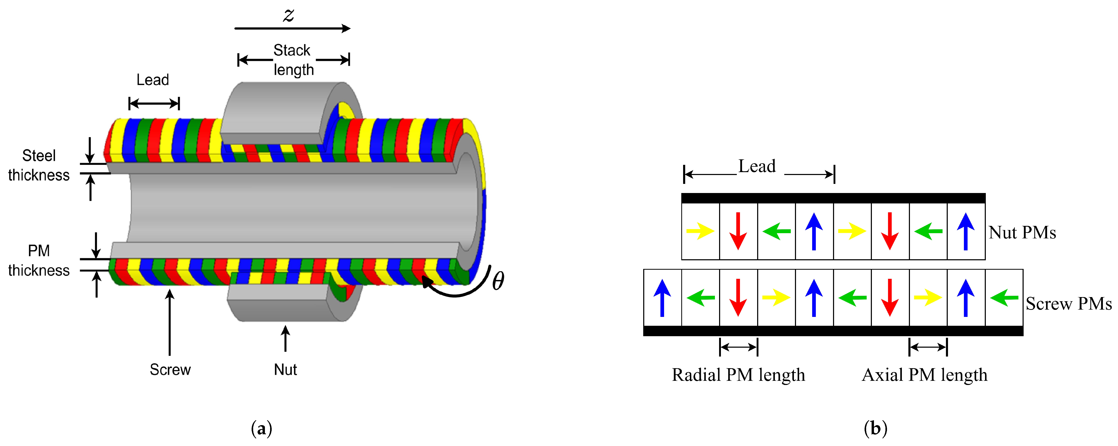
An MLS is a device that converts a high-force, low-speed linear motion into a low-torque, high-speed rotational motion. Hence, this device solves the issues related to machine size and force density [15]. The two primary components of this device are a screw and a nut. The screw and nut are fitted with helical PMs, as illustrated in Figure 2. The device achieves the gearing action while converting between linear and rotational motion using magnetic fields. This makes it possible to convert low-speed, high-force translational motion into high-speed, low-torque rotating motion. A linear displacement equal to twice the magnetic pole pitch is produced in MLSs by a ${360}^{\circ }$ rotation of the nut, and vice versa [15]. Rotating-to-linear magnetic gears are also known as magnetic screws (MSs), rotary-to-linear machines (RotLin), trans-rotary magnetic gears (TROMAG), and MLSs in the literature.

The studies on the modeling and control of the MLS that have been published in the literature are reviewed in this paragraph. A non-linear model is developed to study the performance of MLSs [8]. Additionally, translator oscillation tests are performed to predict the dynamic behavior. In order to assess the system’s dynamic responsiveness to speed commands, the non-linear model is linearized to obtain the transfer function. It is demonstrated that the gear ratio is impacted by the moment of inertia when a reactive control method is employed. In [30], the model is experimentally validated. Applications requiring short strokes and high force are where the MLS excels. A robust position control method that is more reliable and accurate than the traditional control system, which consists of a conventional two-loop structure with an outer mover position control loop and an inner rotor angle speed control loop using proportional controllers, is suggested in [31]. The MLS integrated with a PM brushless machine is intended to be controlled by the system. The stator, nut (rotor), and screw (translator) are, thus, the three primary components of this system. One disturbance observer and two proportional controllers form the foundation of the conventional position control system. The two controller loops are made up of an inner rotor angle speed control loop and an outer mover position control loop. When applied to a 2-mass system, inadequate robustness occurs since the conventional position control mechanism is favored for single inertia systems. Nevertheless, a load force observer based on the estimated spring force between the screw and the nut is part of the position control system in [31]. Additionally, a deflection compensator is used on the load side to guarantee the precision of the position control. In the event of a load disturbance, this compensator modifies the rotor angle. Additionally, by including a feedback loop within the speed control loop, the speed response to abrupt changes in the load force is enhanced. Also, ref. [32] proposed a sliding mode linear speed controller to enhance the dynamic performance of the MLS. As MLS systems regularly require a rotary and linear encoder for accurate positioning, The authors in [33] proposed sensorless position control. It is noticed that in all studies presented in the literature, the translator speed works with a constant or step waveform, and the challenge of controlling a sinusoidal translator speed waveform is addressed in this paper.

This paper presents a theoretical analysis of the idealized Halbach MLS system, contrasting it with the discrete MLS system. Although both systems are non-linear, the discrete MLS torque waveform has more harmonics when compared with the ideal MLS torque waveform [26]. Despite practical challenges in achieving ideal torque/force due to magnet strength and helical structure limitations, this paper provides a foundational framework for developing advanced magnetic lead screws and offers detailed insights into the proposed controller design.

The primary contribution of this paper is the investigation of both classical and advanced control techniques applied to the ideal Halbach MLS for wave energy applications, with the primary objective being to accurately track the translational speed of the MLS in order to maximize the harvested ocean wave energy. The paper is structured as follows. Section 2 details the model of an ideal Halbach MLS. Section 3 discusses the design and simulation results of classical controllers, namely the proportional-integral (PI) and proportional-resonant (PR) controllers. 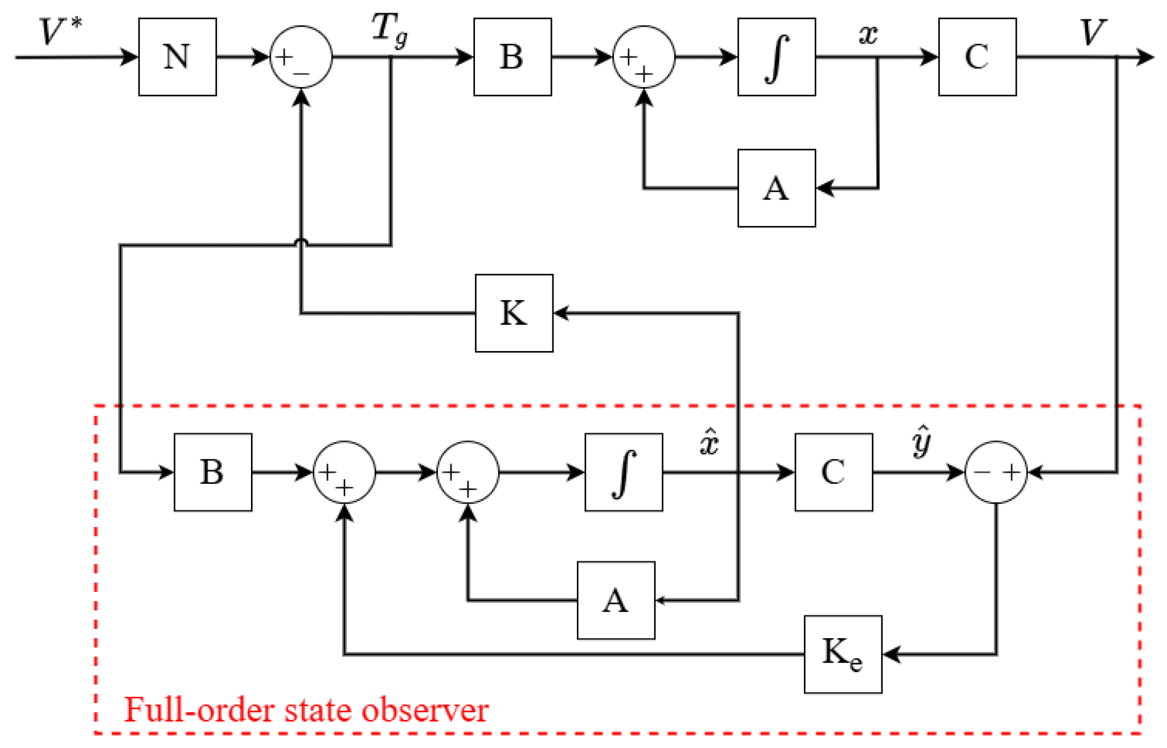Section 4 deals with the design and simulation results of the advanced observer-based state feedback controller (O-SFC). Section 5 compares the performance of the proposed controllers. Finally, Section 6 presents the conclusion.

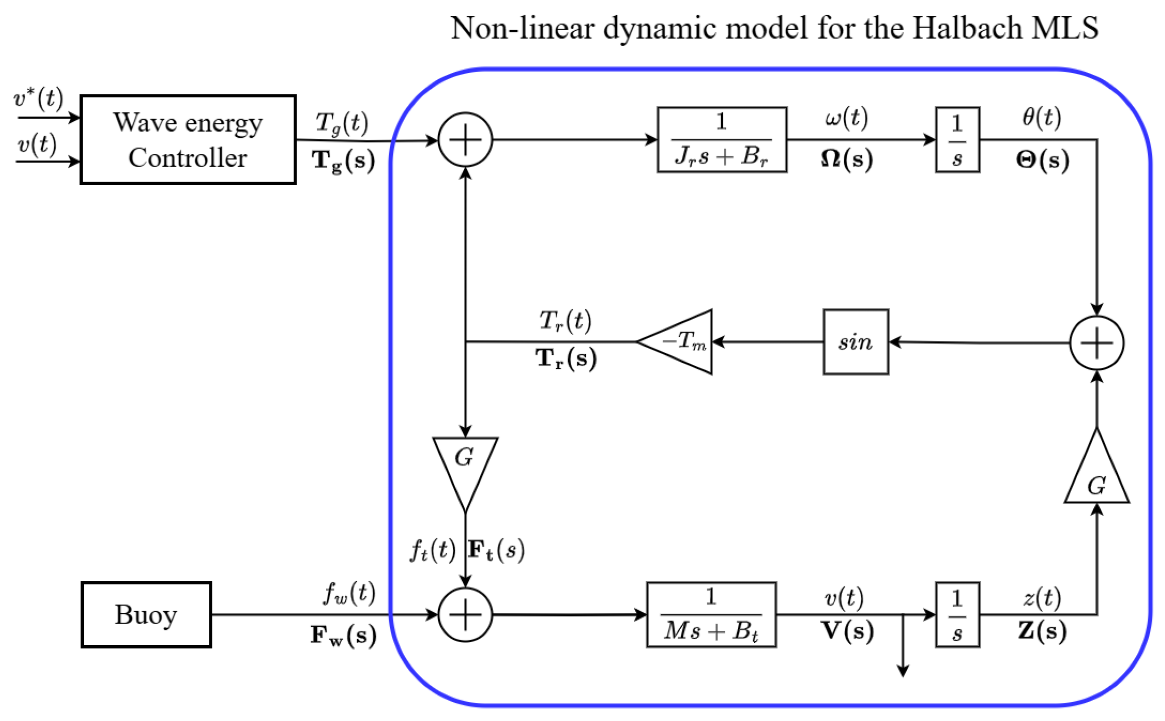
2. Model of the Ideal Halbach Magnetic Lead Screw

In an MLS, the number of poles viewed from the xy-plane is equivalent to the number of starts in the mechanical screw. The Halbach MLS utilizes both radial and axial magnetized PMs, as shown in Figure 2. This special arrangement increases the thrust force capability since it consists of radially magnetized permanent magnets placed between two axially magnetized magnets. The main flux is produced by the radial magnets, and the leakage flux is suppressed by the axial magnets. The lead $\lambda$ is defined as the distance that the screw moves as the nut rotates one cycle. This is equivalent to the product of the number of poles and the magnet width (twice the pole pitch) [34]. This fact leads to the following relationship between the torque T and the thrust force F as,

$$T= {\displaystyle \frac{\lambda }{2\pi }} F$$

(1)

The equivalent magnetic gear ratio G is defined as,

$$G= {\displaystyle \frac{F}{T}}= {\displaystyle \frac{2\pi }{\lambda }}$$

(2)

where $\omega$ is the rotational velocity and v is the linear velocity.

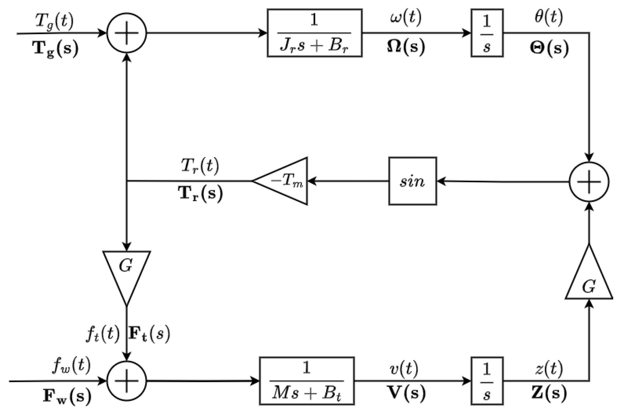
This section deals with the modeling and control of the ideal Halbach MLS. An analytical model derived from a dynamic viewpoint by considering the MLS as a mass-spring system was presented in [8,30]. The equations of motion for the rotor and translator are represented by Equations (3) and (4).

$$J_r\ddot{\theta }\left(t\right)+B_r \dot{\theta }\left(t\right)=T_g\left(t\right)+ T_r\left(t\right)$$

(3)

$$M\ddot{z}\left(t\right)+B_t \dot{z}\left(t\right)=f_t\left(t\right)+ f_w\left(t\right)$$

(4)

In the above two equations, $\theta$ and z are the rotor and the translator positions, respectively. $T_g$, $T_r$, $f_t$, and $f_w$ are the rotating generator torque, the MLS rotor torque, the MLS translator force, and the wave force, respectively. Also, $J_r$ is the moment of inertia of the rotating parts of the MLS, $B_r$ is the damping coefficient associated with the rotation of the rotor, M is the total mass of the translating part, and $B_t$ is the damping coefficient associated with the translating parts.

The MLS formulas for the rotor toque and the translator force are presented in (5), where the stable operating range of the MLS is from $-{90}^{\circ }$ to ${90}^{\circ }$.

$$f_t=G{T}_r =-G{T}_{m}sin(\theta +Gz)$$

(5)

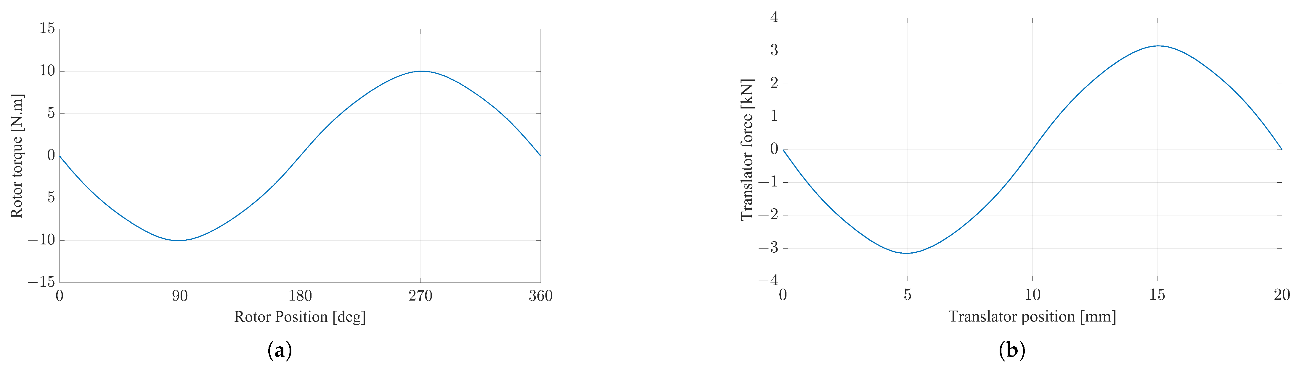
Note that the term $\theta +Gz$ is the relative position between the rotor and the translator. G is $2\pi /\lambda$ and $T_m$ is the peak value of the rotor torque of the MLS, as shown in Figure 3a, which presents the simulation result of an ideal Halbach MLS. The block diagram of the dynamic MLS model is depicted in Figure 4. The ideal Halbach MLS with a radial length of 5 mm and PM thickness of 5 mm is chosen for further analysis and control. The torque and force results for the ideal Halbach MLS represented in (5) are depicted in Figure 3. Therefore, the non-linear model of the system is as follows:

$$J_r\ddot{\theta }\left(t\right)+B_r \dot{\theta }\left(t\right)=T_g\left(t\right)+ T_r\left(t\right)$$

(6)

$$M\ddot{z}\left(t\right)+B_t \dot{z}\left(t\right)=f_t\left(t\right)+ f_w\left(t\right)$$

(7)

$$\dot{z}\left(t\right)=v\left(t\right)$$

(8)

$$\dot{\theta }\left(t\right)=\omega \left(t\right)$$

(9)

Equation (6) corresponds to the top section of the block diagram in Figure 4, while Equation (7) represents the bottom section. The middle section describes the non-linear equation of the MLS, which accounts for both linear and rotational motions. The linearized model is obtained by letting,

$$sin(\theta +Gz)\approx \theta +Gz$$

(10)

The approximation in Equation (10) is valid when the angle $\theta +Gz$ is small. The input is $u=T_g$, and the output of the system is $y=v$. The state space representation of the linearized model of the MLS is as follows, using Equations (5) and (10), is as follows:

$$T_r=-T_m(\theta +Gz)$$

(11)

hence

$$\dot{T_r}=-T_m(\dot{\theta }+G\dot{z})$$

(12)

The chosen states are $T_r$, $\omega$, and v. The state vector is $x={\left[\begin{array}{ccc}{T}_r& \omega & v\end{array}\right]}^T$. Note that $T_r$ is the MLS rotor torque, $\omega$ is the angular velocity, and v is the translator speed. The state space representation of the system can be written as follows,

$$\dot{x}=Ax+Bu+E{F}_w$$

(13)

$$y=Cx$$

(14)

where,

$x=\left[\begin{array}{c}{T}_r\\ \omega \\ v\end{array}\right]$

$A=\left[\begin{array}{ccc}0& -T_m& -T_{m}G\\ {\displaystyle \frac{1}{J_r}}& -{\displaystyle \frac{B_r}{J_r}}& 0\\ {\displaystyle \frac{G}{M}}& 0& -{\displaystyle \frac{B_t}{M}}\end{array}\right],B=\left[\begin{array}{c}0\\ {\displaystyle \frac{1}{J_r}}\\ 0\end{array}\right]$

$E=\left[\begin{array}{c}0\\ 0\\ {\displaystyle \frac{1}{M}}\end{array}\right],C=\left[\begin{array}{ccc}0& 0& 1\end{array}\right]$

Note that $F_w$ represents the disturbance acting on the system. The disturbance will be ignored during the initial analysis, and the transfer function of the MLS system is such that,

$$G\left(s\right)={\displaystyle \frac{V\left(s\right)}{T_g\left(s\right)}}={\displaystyle \frac{-G{T}_m}{a_3{s}^3+a_2{s}^2+a_{1}s+a_0}}$$

(15)

where,

$a_0=B_r{T}_m{G}^2+B_t{T}_m$;

$a_1= J_r{T}_m{G}^2+T_{m}M+B_r{B}_t$;

$a_2=B_t{J}_r+B_{r}M$;

$a_3=J_{r}M$.

The transfer function of the system is a third order because the paper deals with the control of the translating speed.

3. Classical Controllers for Ideal Halbach Magnetic Lead Screw

This section examines two types of controllers: proportional-integral controller and proportional-resonant controller. The design methodologies and simulation results for both controllers are presented in this section.

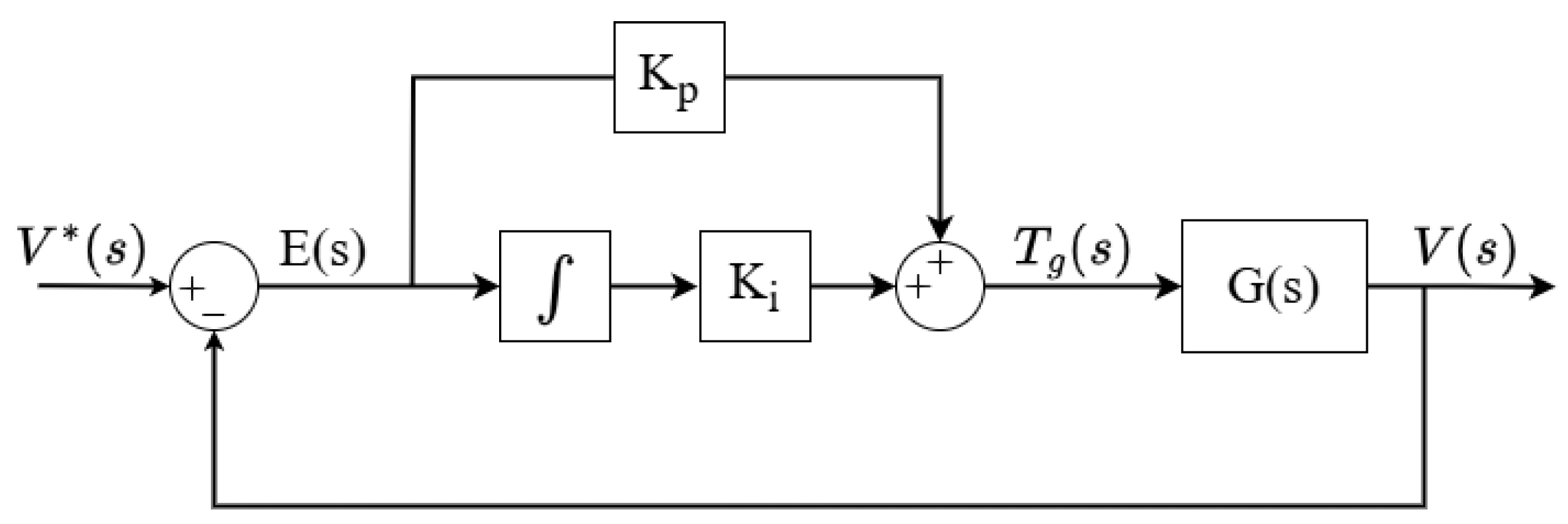
3.1. Design of the Proportional-Integral Controller

The control of the MLS using a proportional-integral controller was presented in [30]. The reference input was a step function. However, since the controller is designed for wave energy applications, the reference speed in this paper is sinusoidal, as the wave is assumed to be monochromatic (steady-state sinusoidal with a single frequency). This achieves maximum power extraction from the float translational to the rotational stage of the PTO, where the translator speed is sinusoidal and in phase with the incoming sinusoidal ocean wave force. For the simulations, an ideal Halbach MLS with a radial length of 5 mm and PM thickness of 5 mm is used. The model specifications given in

Table 1. Magnetic lead screw model specifications.

Quantity	Value	Unit
M	17.15	kg
$J_r$	0.02255	kg·m2
$B_r$	0.002625	N·m·s
$B_t$	89	N·s/m
$T_m$	10	N·m
G	$100\pi$	m−1

are used.

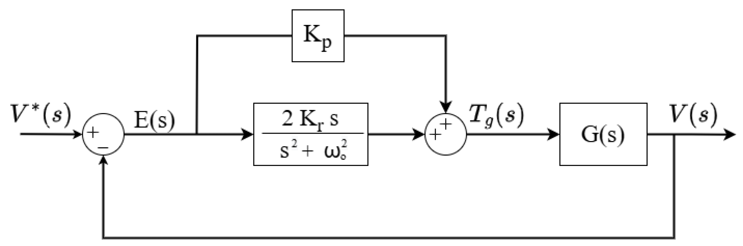
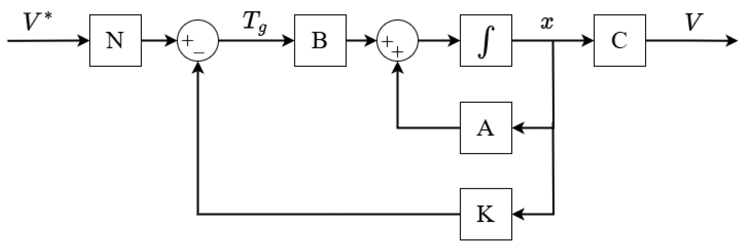
A conventional PI controller for the MLS is designed and simulated as it will serve as a benchmark that can be used to compare with the other proposed controllers. The block diagram of the linearized MLS model controlled using the PI controller is shown in Figure 5. The PI controller transfer function is given by (16).

$$G_{PI}\left(s\right)={\displaystyle \frac{T_g\left(s\right)}{E\left(s\right)}}=K_p+{\displaystyle \frac{K_i}{s}}$$

(16)

$V^{*}\left(s\right)$ is the reference input to the system. The closed-loop transfer function is given in (17).

$${\displaystyle \frac{V\left(s\right)}{V^{*}\left(s\right)}}={\displaystyle \frac{G_{PI}\left(s\right)G\left(s\right)}{1+G_{PI}\left(s\right)G\left(s\right)}}={\displaystyle \frac{-G{T}_m(K_{p}s+K_i)}{a_4{s}^4+a_3{s}^3+a_2{s}^2+a_{1}s+a_0}}$$

(17)

where:

$a_0=-G{K}_i{T}_m$;

$a_1=T_m(B_r{G}^2+B_t-K_{p}G)$;

$a_2=T_m(J_r{G}^2+M)+B_r{B}_t$;

$a_3=J_r{B}_t+B_{r}M$;

$a_4=J_{r}M$.

It is concluded from the Routh–Hurwitz criterion analysis that the stable region for $K_p$ and $K_i$ is $K_p>-38$ and $-62.1\times {10}^3<K_i<0$. In the PI controller design, the intended phase margin is limited to ${30}^{\circ }$ to ${60}^{\circ }$. The gain is regulated to $1.1$ or less, and the phase shift is limited to less than $1^{\circ }$ for no load and at the reference frequency. The gain at the resonance frequency is set to 5 or less in order to reduce the ripple. Only a gain crossover frequency of 8 rad/s and a phase margin of ${30}^{\circ }$ can be verified to meet these requirements. The gain margin that results is 2.48 dB. The ripple grows when the gain or phase shift is minimized. The resulting $K_p$ and $K_i$ are $-27.6$ and $-399.5$, respectively, which are located in the stable area.

3.2. Simulation Results of the PI-Controlled Magnetic Lead Screw System

The reference speed is defined as a sine function with an initial amplitude of 0.1 m/s, which is later increased to 0.4 m/s. The sine function has a frequency of 2 rad/s. To maximize the extracted power, both the reference speed and the wave force are kept in phase. This torque is controlled to regulate the MLS, which is driven by an electrical machine. The wave force is defined as follows, $f_w\left(t\right)=F_{peak} sin(\omega t)$. According to Figure 3, the maximum translator force is approximately 3 kN. However, to ensure safety and prevent the MLS from slipping, the full wave force peak value is set at 2.8 kN. The peak wave force varies with each reference speed, ranging from no wave force to $F_{peak}=1.4$ kN ($50\%$ of the maximum wave force) and $F_{peak}=2.8$ kN. Additionally, based on the electrical machine’s specifications, the torque $T_g$ is constrained to 11.5 N·m. Introducing this torque constraint to the MLS model adds a practical aspect to the system’s design.

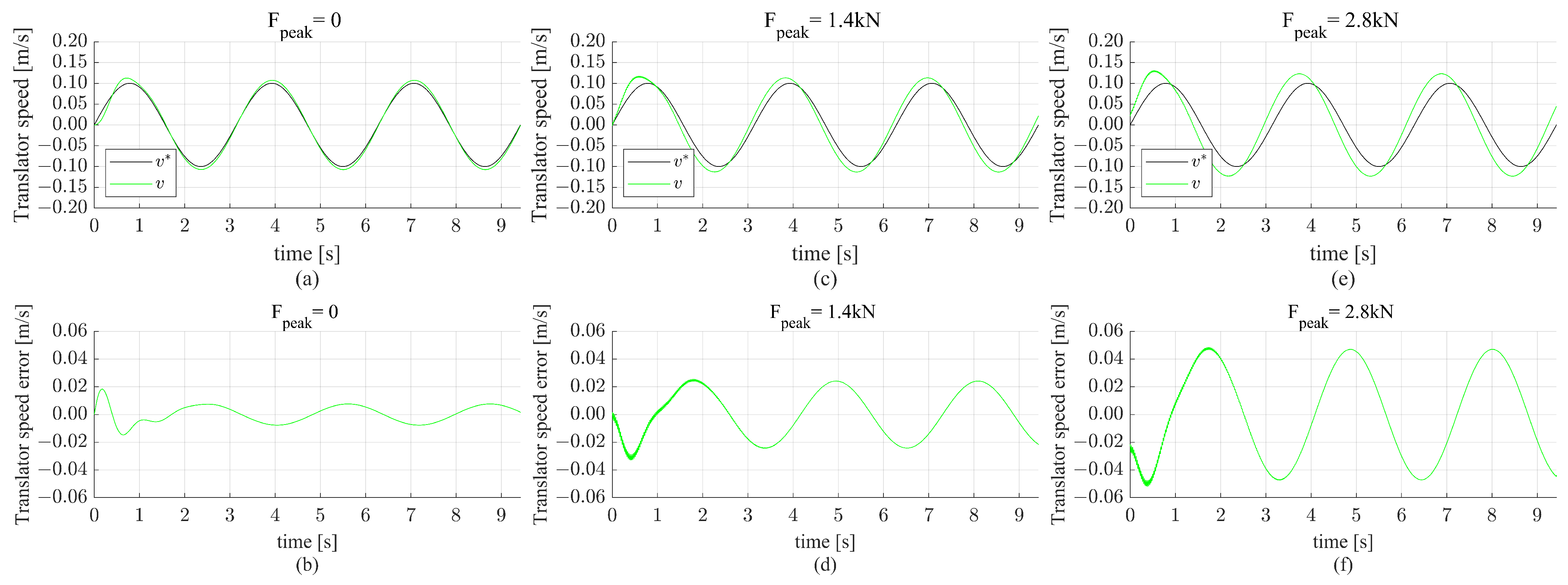
The simulation results for both the linear model (the controller is designed based on the linear model) and the non-linear model will be presented. The simulation results of the controlled linear model are included to show that the controller is designed correctly at no wave force (disturbance). The block diagram of the non-linear Halbach MLS model, including the controller, is presented in Figure 6.

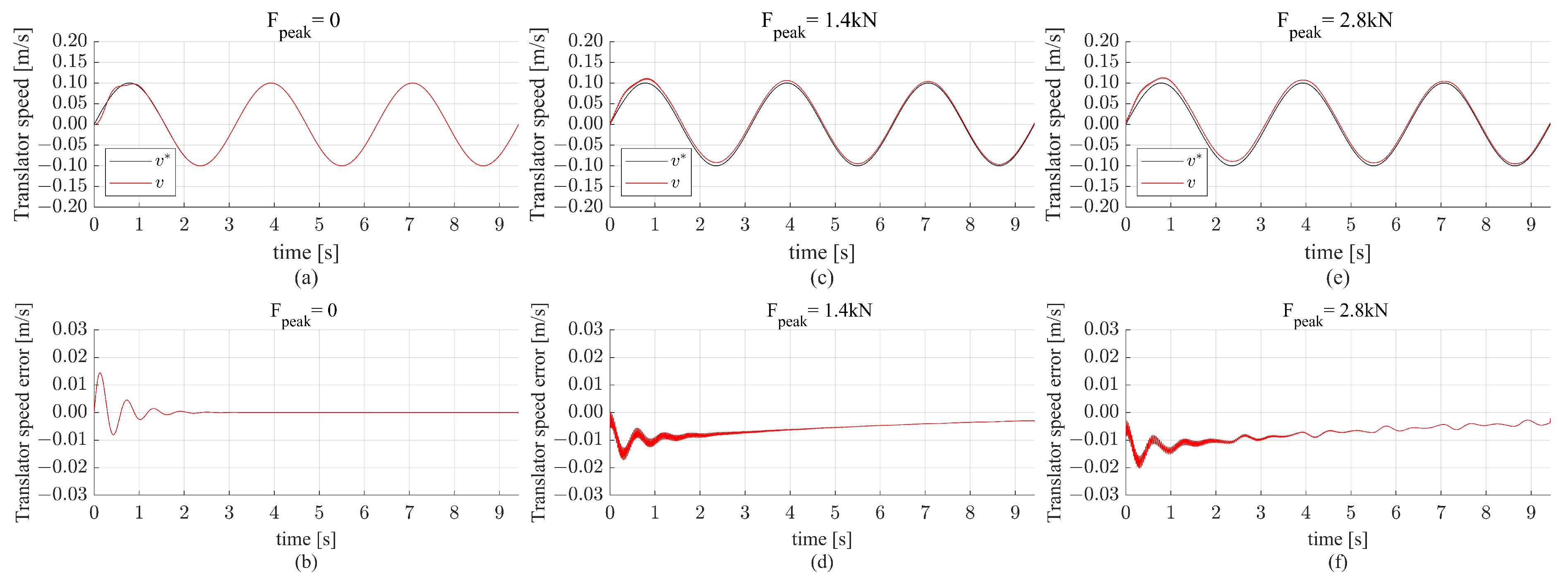
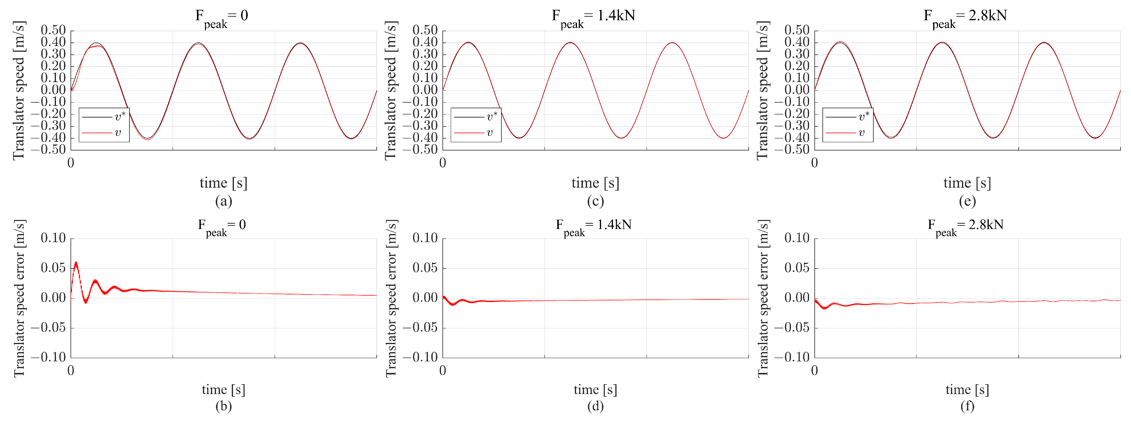
The simulation results with a sine reference speed with 0.1 m/s magnitude and the three wave forces for the linear model are shown in Figure 7. It is clear from Figure 7a that for $F_{peak}=0$, the design requirements are satisfied, and the translator speed is tracked accurately. The translator speed error shown in Figure 7b does not exceed $0.01$ m/s in the case of $F_{peak}=0$. As the wave force increases, the translator’s speed tracking accuracy decreases. This is illustrated in Figure 7c,d for $F_{peak}=1.4$ kN, where the maximum error increased to approximately $0.02$ m/s. The error increased even more when $F_{peak}=2.8$ kN, as shown in Figure 7f.

Moreover, the exact simulation conditions are replicated in the non-linear model. The results are shown in Figure 8. The results obtained are quite close to the results of the linear model simulation. The translator speed is shifted and has a higher amplitude than the reference speed in case of disturbance ($F_{peak}$). The translator speed error in the cases of $F_{peak}=1.4$ kN and $F_{peak}=2.8$ kN are approximately equal to $0.024$ m/s and $0.047$ m/s, respectively, in steady state. This is shown in Figure 8d,f. 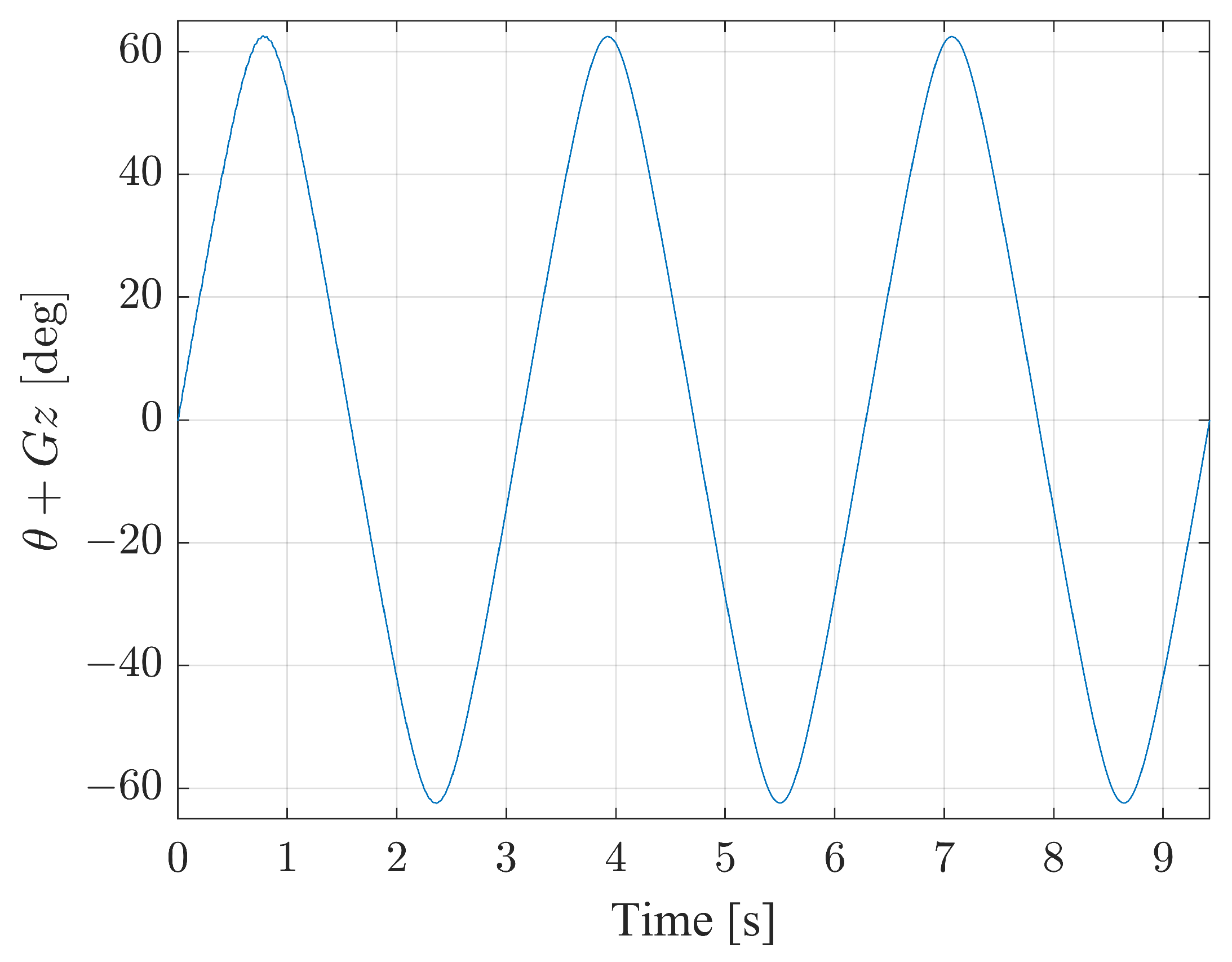Figure 9 shows $\theta +Gz$ at the highest wave force peak, where $\theta +Gz$ reaches its maximum value, demonstrating that even under the most extreme conditions, the angle remains within the stable operating range.

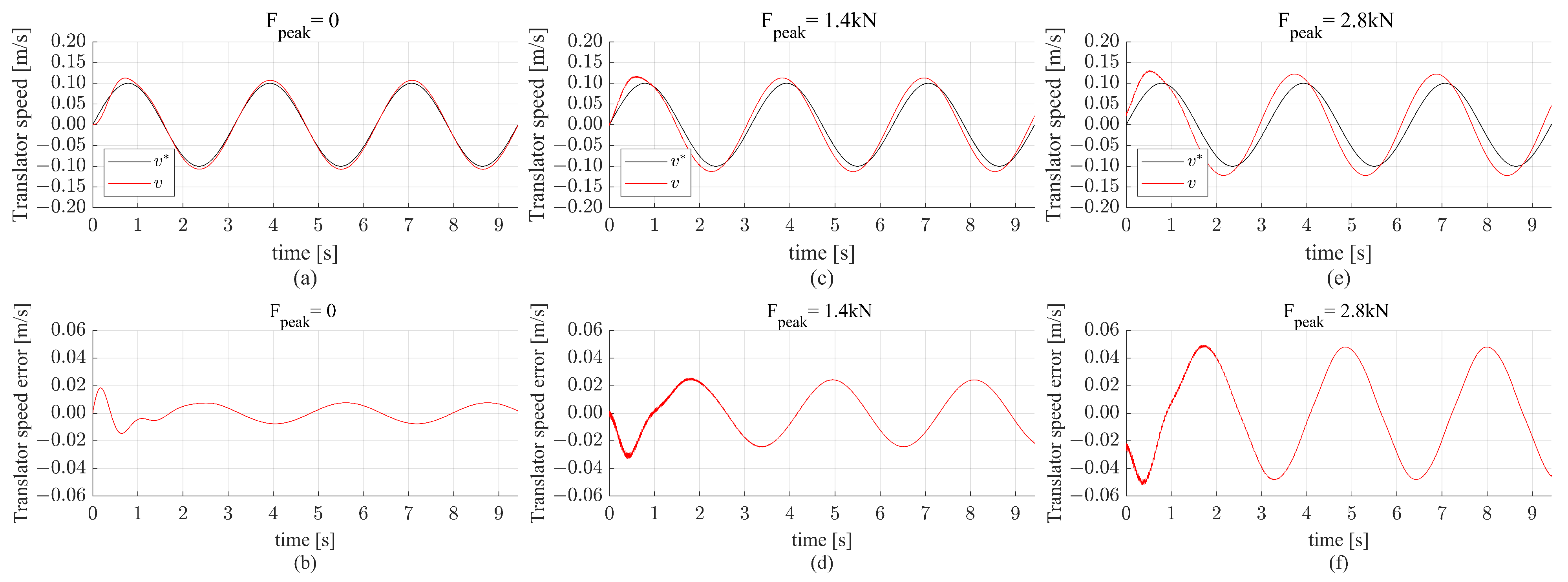
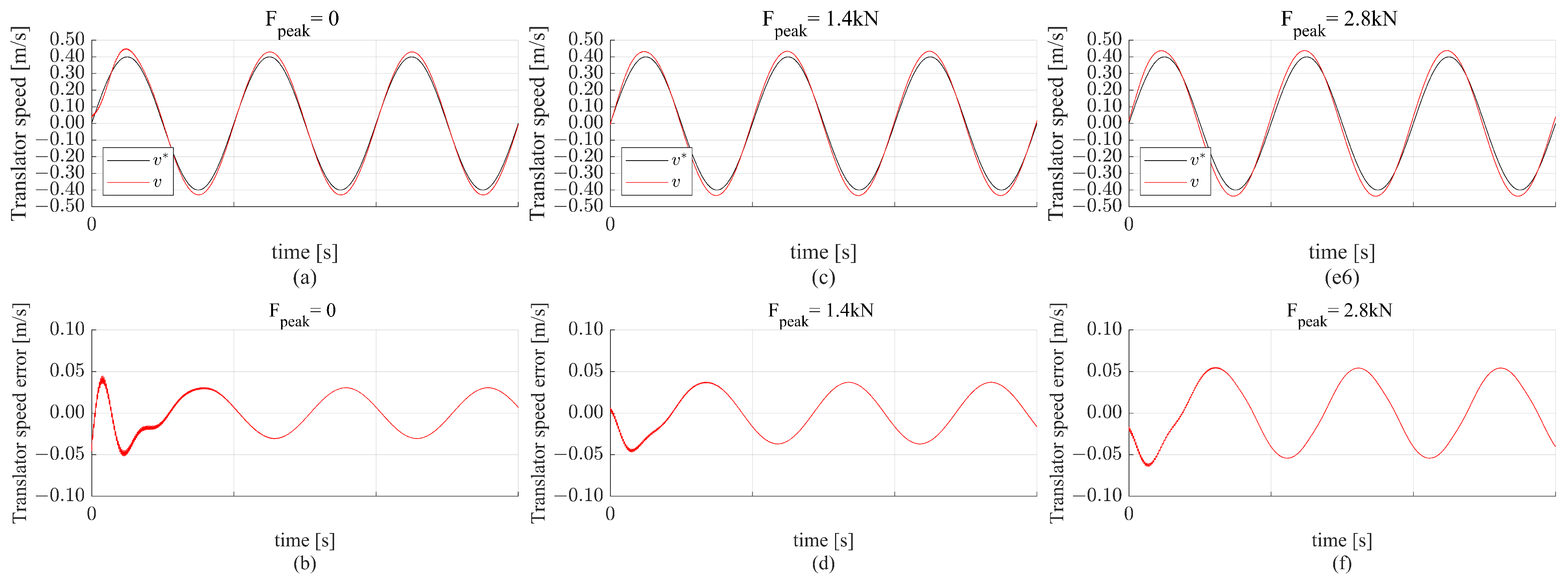
For the remaining simulations, the results are presented for the non-linear model, since it is the practical model, as shown in Figure 6. The PI controller is also tested for the sine reference speed with a magnitude of $0.4$ m/s with the three wave forces, as shown in Figure 10. The reference speed tracking is slightly less accurate compared to the reference speed magnitude of $0.1$ m/s. However, in all cases, the translator speed error does not exceed $0.06$ m/s, and the phase shift between the reference and the translator speed is less compared to the case with a reference speed magnitude of $0.1$ m/s.

Clearly, the PI controller is not well suited for a sinusoidal reference speed and is highly affected by disturbance. Therefore, the proportional-resonant controller is investigated.

3.3. Design of the Proportional-Resonant Controller

For single-phase AC current or voltage regulation, the proportional-resonant controller has drawn a lot of interest in the field of power electronics. It is frequently used in sinusoidal waveform systems, which makes MLS systems a perfect fit. Ref. [35] presented the proportional-resonant controller’s mathematical derivation. The block diagram of the linearized MLS model controlled by a proportional-resonant controller is shown in Figure 11.

The transfer function for the proportional-resonant controller is provided by,

$$G_{PR}\left(s\right)={\displaystyle \frac{T_g\left(s\right)}{E\left(s\right)}}=K_p+{\displaystyle \frac{2K_{r}s}{s^2+{{\omega }_o}^2}}$$

(18)

where ${\omega }_o$ refers to the targeted frequency. Therefore, ${\omega }_o$ is chosen to be the same as the wave $\left(V^{*}\right)$ frequency since it is the targeted reference. Also, $K_p$ and $K_r$ represent the controller gains. The closed-loop transfer function is given by (19). Note that substituting s by $j{\omega }_o$ results in a gain of 1 and 0 phase shift.

$$\begin{array}{cc}\hfill {\displaystyle \frac{V\left(s\right)}{V^{*}\left(s\right)}}& ={\displaystyle \frac{G_{Pr}\left(s\right)G\left(s\right)}{1+G_{Pr}\left(s\right)G\left(s\right)}}\hfill \\ & ={\displaystyle \frac{-G{T}_m(K_p{s}^2+2K_{r}s+K_p{\omega }_0^2)}{a_5{s}^5+a_4{s}^4+a_3{s}^3+a_2{s}^2+a_{1}s+a_0}}\hfill \end{array}$$

(19)

where:

$a_0={{\omega }_o}^2{T}_m(B_t-G{K}_p+B_r{G}^2)$;

$a_1={{\omega }_o}^2(B_r{B}_t+M{T}_m+T_m{J}_r{G}^2)-2G{T}_m{K}_r$;

$a_2=T_m(B_r{G}^2-K_{p}G+B_t)+{{\omega }_o}^2(J_r{B}_t+B_{r}M)$;

$a_3=J_r(T_m{G}^2+M{{\omega }_o}^2)+B_r{B}_t+M{T}_m$;

$a_4=J_r{B}_t+B_{r}M$;

$a_5=J_{r}M$.

Using the Routh–Hurwitz criterion, the stable region for $K_p$ is $-37<K_p<1.1$. $K_p$ is chosen to be $-27.6$, which lies in the stable region. For that value of $K_p$, the $K_r$ stable region is $-37\times {10}^3<K_r<0$; $K_r$ is chosen to be $-399.5$. As shown in the closed loop transfer function, the PR controller outputs a gain of 1 and a phase shift of 0 as long as the chosen $K_p$ and $K_r$ lie in the stable region. The resulting phase margin is equal to ${21}^{\circ }$, and the resulting gain margin is equal to $2.5$ dB.

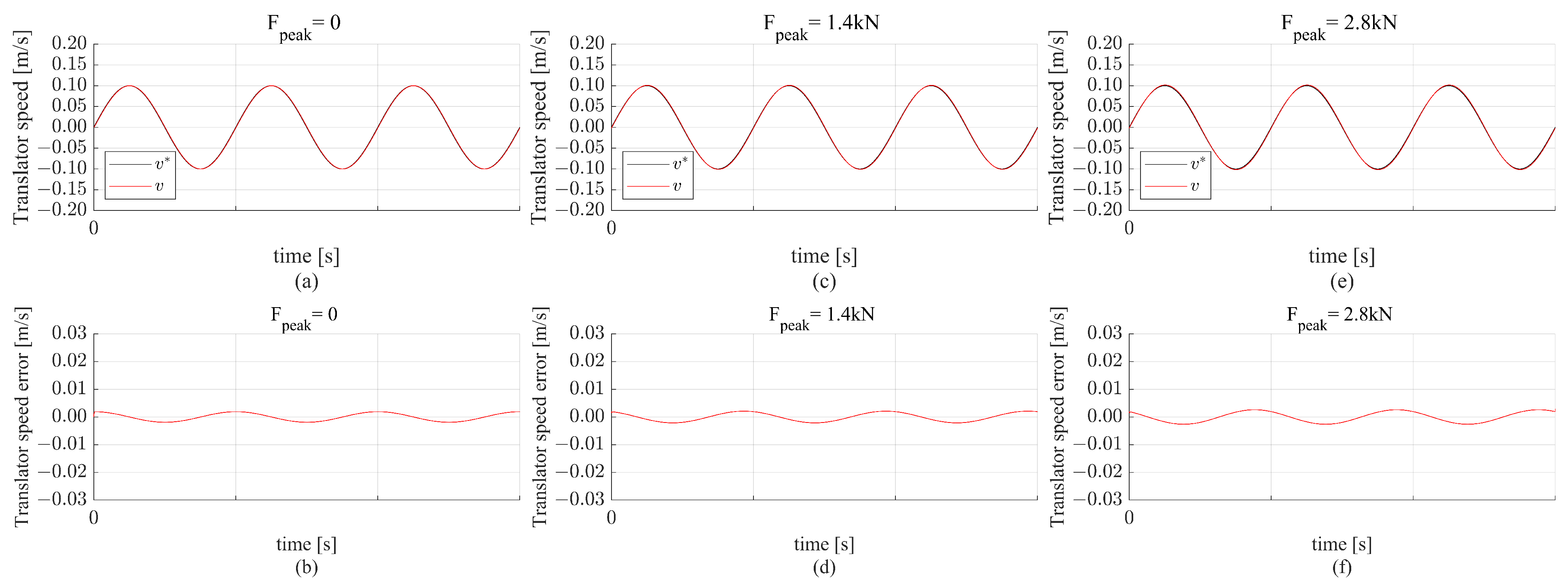
3.4. Simulation Results of the PR-Controlled Magnetic Lead Screw System

The PR controller is tested under the same conditions applied to the PI controller. The simulation results of the non-linear model with varying $F_{peak}$ and a reference speed magnitude of 0.1 m/s are shown in Figure 12. It is clear that in condition $F_{peak}=0\%$, the translator speed accurately tracks the reference speed where the translator speed error shown in Figure 12b is equal to zero. For the $F_{peak}=1.4$ kN, the resulting translator speed is in phase with the reference speed with a slight increase in the gain. The translator speed error is approximately equal to $0.003$ m/s in the case of $F_{peak}=2.8$ kN.

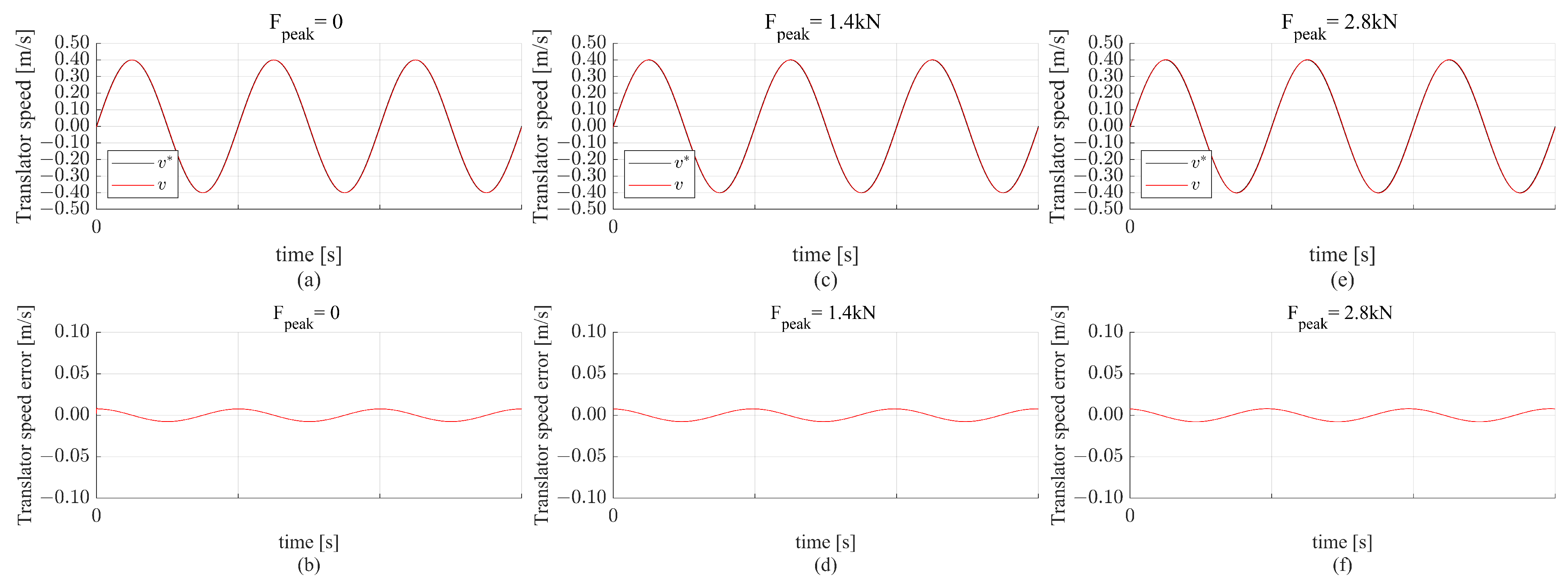
Similarly, the controller is tested for a reference speed magnitude of 0.4 m/s. The simulation results for the non-linear model are shown in Figure 13. It is clear that in the case of $F_{peak}=0$, the translator speed error slightly increased to $0.005$ m/s when compared to the reference speed magnitude of 0.1 m/s. Also, The translator speed error for the $F_{peak}=1.4$ kN and $F_{peak}=2.8$ kN wave force is approximately equal to $0.0016$ m/s and $0.0033$ m/s, respectively. The command torque in the presence of disturbances for all conditions is within the physical limits of the system.

It is clear from the simulation results that the MLS system controlled using the PR controller gave much better results than the PI-controlled MLS system.

4. Advanced Controller for Ideal Halbach Magnetic Lead Screw

This section focuses on the design of an observer-based state feedback controller for the ideal Halbach MLS linear model. The designed controller is simulated using the non-linear model.

4.1. Design of Observer-Based State Feedback Controller

A state feedback controller’s block diagram representation is shown in Figure 14. Equations (20) and (21) provide the MLS system’s state space representation. The input u for the state feedback controller is given by Equation (22). The gain K is a $3\times 1$ matrix given by (23). The parameters $K_{T_r}$, $K_{\omega }$, and $K_v$ represent the state feedback gains.

$$\dot{x}=Ax+Bu$$

(20)

$$y=V=Cx$$

(21)

$$T_g=-Kx+Nr$$

(22)

where,

$$K=\left[\begin{array}{ccc}{K}_{T_r}& K_{\omega }& K_v\end{array}\right]$$

(23)

The closed-loop system is such,

$$\dot{x}=Ax+B(-Kx+Nr)=(A-BK)x+BNr$$

(24)

$$\dot{x}=A_{c}x+B_{c}r$$

(25)

where, $A_c=(A-BK)$; $B_c=BN$.

The closed-loop transfer function of the system is as follows,

$$G_a\left(s\right)={\displaystyle \frac{V\left(s\right)}{V^{*}\left(s\right)}}=C{(sI-A_c)}^{-1}{B}_c$$

(26)

$$G_a\left(s\right)={\displaystyle \frac{V\left(s\right)}{V^{*}\left(s\right)}}={\displaystyle \frac{-GN{T}_m}{a_3{s}^3+a_2{s}^2+a_{1}s+a_0}}$$

(27)

where,

$a_0=T_m(B_r{G}^2+B_t+B_r{G}^2+G^2{K}_{\omega }-B_t{K}_{T_r}-G{K}_v)$

$a_1=T_m(J_r{G}^2+M-M{K}_{T_r})+B_r{B}_t+B_t{K}_{\omega }$

$a_2=M{B}_r+J_r{B}_t+M{K}_{\omega }$

$a_3=J_{r}M$

The parameters $K_{T_r}$, $K_{\omega }$, and $K_v$ are determined such that the closed loop poles are in the left-half plane. Table 1 contains the MLS system’s parameters. The controller’s poles are placed at $-150$ rad/s, $-700$ rad/s, and $-700$ rad/s, resulting in the following gains: $K_{T_r}=-1426$, $K_{\omega }=34.8$, and $K_v=2322$. The gain N is obtained using the following equation.

$$N={\displaystyle \frac{-1}{C{(A-BK)}^{-1}B}}$$

(28)

The purpose of a full-state observer is to minimize the quantity of sensors required. Figure 15 displays the block diagram of the MLS system with the observer and controller, where $K_e$ represents the observer’s gain. Equations (29) and (30) provide the representation of the observed state space. The 3×1 matrix gain $K_e$ is determined by (31). The observer states gains are represented by the parameters $K_{T_{r}obs}$, $K_{\omega obs}$, and $K_{vobs}$. The observer’s poles are positioned more to the left of the controller’s dominant poles. The observer’s poles are as follows: −6000, −6000, −6000 $rad/s$. The following part presents the MLS system’s simulation results using the observer-based state feedback controller.

$$\dot{\widehat{x}}=A\widehat{x}+Bu+K_e(y-\widehat{y})$$

(29)

$$\widehat{y}=C\widehat{x}$$

(30)

$$K_e=\left[\begin{array}{ccc}{K}_{T_{r}obs}& K_{\omega obs}& K_{vobs}\end{array}\right]$$

(31)

4.2. Simulation Results of the Observer-Based State-Feedback-Controlled Magnetic Lead Screw System

The controller is initially tested using the linear MLS model (design-based model) to ensure proper controller design. Subsequently, it is tested on the non-linear model. Only the results from the non-linear model are presented. The simulation results for a reference speed of a 0.1 m/s magnitude with varying wave forces are shown in Figure 16. The results demonstrate that the controller accurately tracks the reference speed, maintaining a translator speed error close to zero across all wave forces, indicating good performance. To further evaluate the controller, it was tested with a reference speed of 0.4 m/s magnitude under the same wave conditions. The results, illustrated in Figure 17, show that the controller’s performance remains excellent, matching the high level of accuracy observed with a reference speed of 0.1 m/s magnitude.

5. Comparison Between the Classical and Advanced Controllers

This section presents a comparison between the three controllers. It is evident that the PI controller is less suitable for sinusoidal reference tracking compared to the other two proposed controllers. A comparison of the three controllers is presented in

Table 2. Comparison between the presented controllers for the non-linear Halbach MLS model.

	PI-Controller	PR-Controller	O-SFC Controller
Reference tracking accuracy	Low	High	High
Maximum reference tracking error	High	High	Low
Transient response time	Slow	Slow	Fast
Number of sensors needed	2	2	1

. The controllers are evaluated based on reference tracking accuracy, maximum reference tracking error, transient response time, and the number of sensors required. It is clear that the PI controller is not well suited for sinusoidal reference tracking; however, for the two proposed controllers:

• The reference tracking accuracy of both proposed control methods is high under all tested conditions, with the translator speed error not exceeding $0.01$ m/s;
• The maximum reference tracking error is lowest for the O-SFC;
• The O-SFC outperforms in terms of the speed of the response across all conditions and reference speeds, as the PR controller takes longer to reach steady-state conditions;
• The PR controller requires two sensors: a translator speed sensor and a force sensor. In contrast, the O-SFC requires one sensor only, the force sensor, as it eliminates the need for a speed sensor by using an observer. This reduction in sensor requirements makes the O-SFC more cost-effective.

6. Conclusions

The MLS utilizes permanent magnets to convert between linear and rotational motions, offering a gearing action that facilitates the transformation of high-speed, low-torque rotational motion into low-speed, high-force translational motion. This capability makes the MLS particularly well-suited for ocean wave energy applications, where it efficiently converts the oscillatory motion of waves into electrical energy.

In this study, the effectiveness of two controllers, proportional-resonant and observer-based state feedback, is evaluated for an ideal Halbach MLS. A proportional-integral controller is also employed as a benchmark to compare the performance of the proposed controllers. These controllers are developed based on the linearized model of the ideal Halbach MLS and validated through simulation studies involving both linear and non-linear MLS models. The relative error percentage of the PR and O-SFC controllers improved by $95.6\%$ for the PR controller and $85.6\%$ for the O-SFC. These values are obtained for the worst-case scenario, which corresponds to a reference speed of 0.4 m/s and full wave force. The findings reveal that the PI controller is inadequate for the system’s demands. Conversely, both the PR and O-SFC controllers exhibit significant improvements in system performance. However, the O-SFC controller demonstrates lower transient error, requires fewer sensors, and achieves a faster transient response time compared to the PR controller, making it a more efficient choice. This study’s primary contribution lies in demonstrating the superior performance of the O-SFC controller in extracting energy from wave motion using MLS technology.

7. Future Work

Future work will focus on the experimental verification of the conclusions. Moreover, this study will be extended to investigate and compare its findings with various MLS topologies, providing deeper insights into their performance. Further studies will focus on designing non-linear controllers, such as sliding mode controllers and model predictive controllers, for the non-linear model of the MLS. Additionally, the investigation will be expanded to include practical ocean waveforms (non-monochromatic) to better reflect real-world conditions.