Model-Based Design and Evaluation of State-of-the-Art Thermal Management Systems for Electrified Trucks

Abstract

Electric vehicle thermal management systems have in the last two decades grown to become complex systems. This development has come as a response to the unique challenges faced by electrified powertrains, particularly the driving range reduction in cold climate operation. The rapid increase in complexity makes the systems harder to design, control, and evaluate, and consequently, a need for systematic analysis and design tools has emerged. The key contribution of this work is a model-based simulation tool developed to enable the combined evaluation and control of state-of-the-art thermal management systems. To show how engineers may use the tool to solve industrially relevant problems, two simulation case studies are performed and presented. The first case study compares three thermal management system layouts of increasing complexity and shows how their performance varies as ambient temperature decreases. The second case study concerns the potential benefits of additional cooling radiators for fuel cell trucks under heavy load in hot climates.

1. Introduction

In terms of efficiency, electric vehicles carry multiple advantages compared to their conventionally powered counterparts, though many challenges yet remain for their complete adoption. One of these challenges is the growing importance of the onboard thermal management systems (TMSs). These systems have over the last twenty years become significantly more complex to meet the unique thermal challenges that come with electrification.

1.1. Thermal Management Challenges for Electric Vehicles

For battery electric vehicles, one of the main drivers of their development was the driving range reduction suffered in cold climates. From a pure energy management perspective, a disadvantage of combustion engines is their low efficiency. However, from a thermal management perspective, this inefficiency is convenient, as it provides conventional vehicles with an almost inexhaustible source of waste heat. The vehicle’s TMS can then use the waste heat for cabin heating at no additional fuel cost. In lacking this heat source, early electric vehicle designs used electric heaters as a substitute, which drastically reduced the total driving range. For example, reductions as large as 42.8% were reported by [1] for ambient temperatures of −7 °C and below. For consumers in locations experiencing cold winters, this temperature-induced loss of range was a common argument against the purchase of electric vehicles [2].

Electric heaters are inefficient in that for each unit of heat produced, the device expends the same unit of electric work. Heat pumps, in contrast, move heat at a ratio of heat moved per unit of electric work consumed that is greater than one. Today, heat pumps have been adopted in recent state-of-the-art electric vehicle TMSs like the Tesla Model 3 [3] and the Volkswagen ID.4 [4], increasing the driving range in cold climates but also contributing to a growth in system complexity.

Waste-heat recovery is an additional method of improving the driving range in cold climates. There are conditions where the electric machine and power electronic systems require cooling, while the battery and cabin compartment require heating, a natural solution being that the TMS should move heat from the motor and electronics to the battery and cabin systems. Waste-heat recovery can reduce the power requirement of air-source heat pumps, but the resulting gains in efficiency require additional components and fluid connections, which further increases the system complexity.

Battery pack size has a negative impact on the cargo capacity of class 8 trucks [5]: a larger battery increases the range, but also the price and weight. To avoid this trade-off, fuel cell hybridization is considered as a potential solution, due to the higher gravimetric energy density of pressurized hydrogen over battery cells [6,7]. While fuel cell systems are generally lighter, several technical challenges hinder their adoption. One of these challenges is the risk of overheating under heavy load and hot climate conditions.

Fuel cell systems may reach higher efficiencies than combustion engines, yet despite producing less waste heat, the cooling challenge of fuel cell systems is significantly more difficult. This situation comes from the lower operating temperatures and the relatively low exhaust gas enthalpy (see Section 1.1 in [8] and the references cited therein for a discussion on the fuel cell energy balance). It follows that when compared to conventional trucks, the TMS of fuel cell hybrids needs to deal with a significantly higher cooling load.

1.2. Scientific Contribution

Extensive research in electric vehicles’ thermal management has been targeting the component level. Multiple review articles are available on the thermal management of battery systems [9,10,11,12], electric machines [13,14,15], power electronics [16,17,18], and fuel cell systems [19]. However, sustainable solutions for electromobility with electric vehicles are not only about batteries, power electronics, and electric machines. The complete vehicle is an integration of multiple systems that are necessary for coping with the vehicle’s environment and operation. In this context, thermal systems are important for electric vehicles for several reasons, such as temperature management, safety, driver comfort, efficiency, and environmental factors.

An intelligent TMS in electric vehicles is essential, as it has a major influence on vehicle performance, such as driving range and climate comfort, which are related to customer satisfaction. The system must satisfy the different thermal requirements of the vehicle’s components and the vehicle cabin, while also coping with the vehicle’s environment and operation. While designing the TMS for electric vehicles, many different objectives, often conflicting, need to be considered. To find the optimal system configuration, it is necessary to consider all subsystems and component interactions in an integrated manner. For this purpose, the development of novel model-based methodologies that can capture and predict the thermal system’s behavior with high fidelity can make an essential contribution towards sustainable electromobility.

In a previous work [20], the electrochemical commercial vehicle (ECCV) platform was introduced. Therein, models were developed for the electrochemical, mechanical, and gas exchange systems commonly featured on battery electric and fuel cell hybrid vehicles, with a focus on heavy-duty trucks. The guiding philosophy was to build control-oriented, lightweight, and modular component models, yet with sufficient fidelity to simultaneously enable rapid prototyping of hardware designs and control algorithm development in a single simulation environment.

To the authors’ knowledge, there is currently no available simulation environment that fill the same gap as the ECCV platform. For example, simulation environments like FASTSim (version 2.1.4) [21] use set velocity profiles and characterizes vehicles by a minimum selection of parameters. This approach enables fast calculation but is unsuitable for mission planning algorithm development where velocity is an important variable. On the other end of the spectrum of complexity, GT-SUITE [22] provides vehicle models with high fidelity, including numerical solution of one-dimensional flow in manifolds. Although powerful, the software is proprietary and closed source. The Matlab/Simulink tool presented in [23] is, as FASTSim, a backwards simulation approach where the speed profile is again fixed.

In this work, the ECCV platform is extended with the capability to model state-of-the-art TMSs, specifically including the technologies presented in the schematics presented below. In addition, two simulation case studies are performed to highlight how the platform can guide the development of TMS design. The first case study considers the energy-versus-complexity trade-off of electric heating, heat pumps, and waste-heat recovery systems for heavy-duty battery electric trucks. The second case study considers the thermal management performance gains associated with additional radiators for heavy-duty fuel cell trucks.

1.3. Outline

In Section 2, a research literature and patent survey of TMSs is presented as a set of system diagrams, consolidating the academical and industrial view of what state-of-the-art TMSs look like, and provides the modeling objectives for the following section. The modeling methodology is then presented in Section 4, first from a high-level perspective, followed by a selection of component models where additional details are considered. In Section 5, the case studies and their objectives are presented along with the vehicle specifications for each case. The results of the case studies follow, where trade-offs between system complexity, efficiency, and performance are discussed.

2. Literature and Patent Survey of Vehicular Thermal Management Systems

The size and complexity of onboard TMSs have grown significantly over the last two decades, partly in response to the challenges mentioned above. Consequently, they have become harder to design and control. To provide an overview of how these systems have developed, and to provide an introduction to electric-vehicle thermal management, a sequence of schematics of relevant system architectures were synthesized and are here presented along with a brief discussion of their operation.

The schematics shown below are based on the research literature and a patent survey conducted by the authors. Academic publications [24,25,26,27,28,29,30,31,32,33,34,35,36,37,38,39,40,41,42,43,44] and recent patents [45,46,47,48,49,50,51,52,53,54,55,56,57,58,59,60,61,62] (from automakers Rivian, DAF, FORD, GM, Nikola, Volvo, Toyota, Hyundai, and Renault) investigating or comparing TMS architectures were considered and the systems presented within sorted into a number of archetypes which became the basis of the schematics shown below. The goal of the survey was to investigate what academia and industry considered as state-of-the-art TMSs.

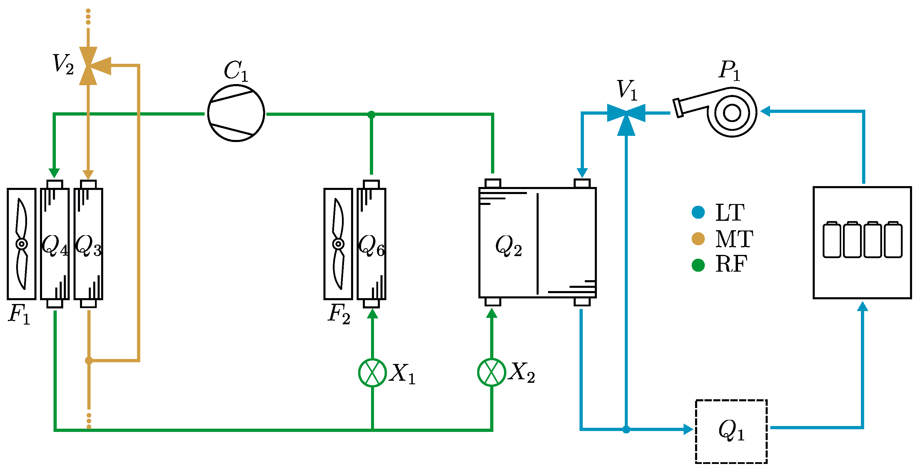
Figure 1 shows an early TMS design with a considerable range reduction in cold climates. The system carries three fluid loops: a low temperature (LT) circuit for cooling the battery pack, a medium temperature (MT) circuit for cooling the motor and power electronics (not shown in the figure), and a refrigerant (RF) circuit tasked to transfer heat from the battery loop to the ambient environment, through the chiller ($Q_2$) and the condenser ($Q_4$).

The reason for using a refrigeration cycle to cool the battery is that common battery temperature setpoints are below the ambient temperature, which requires the movement of heat against the temperature gradient. A compression device ($C_1$) pressurizes the refrigerant such that the boiling point is fixed to 5–10 °C higher than ambient. The pressurized hot gas dissipates heat in the condenser $\left(Q_4\right)$ as it changes phase. The reverse process then occurs: an expansion device $X_1$ lowers the pressure, fixing the boiling point to 5–10 °C lower than the low-temperature loop. Heat transfers from the coolant to the refrigerant loop as the refrigerant evaporates in $Q_2$. The net effect is a transfer of heat from the low-temperature loop to the ambient environment, at the price of the compression work. $V_1$ and $V_2$ are bypass valves used to control their respective coolant circuit’s temperatures. The system in Figure 1 has only one component capable of heating, an electric heater $Q_1$, located in series with the battery pack.

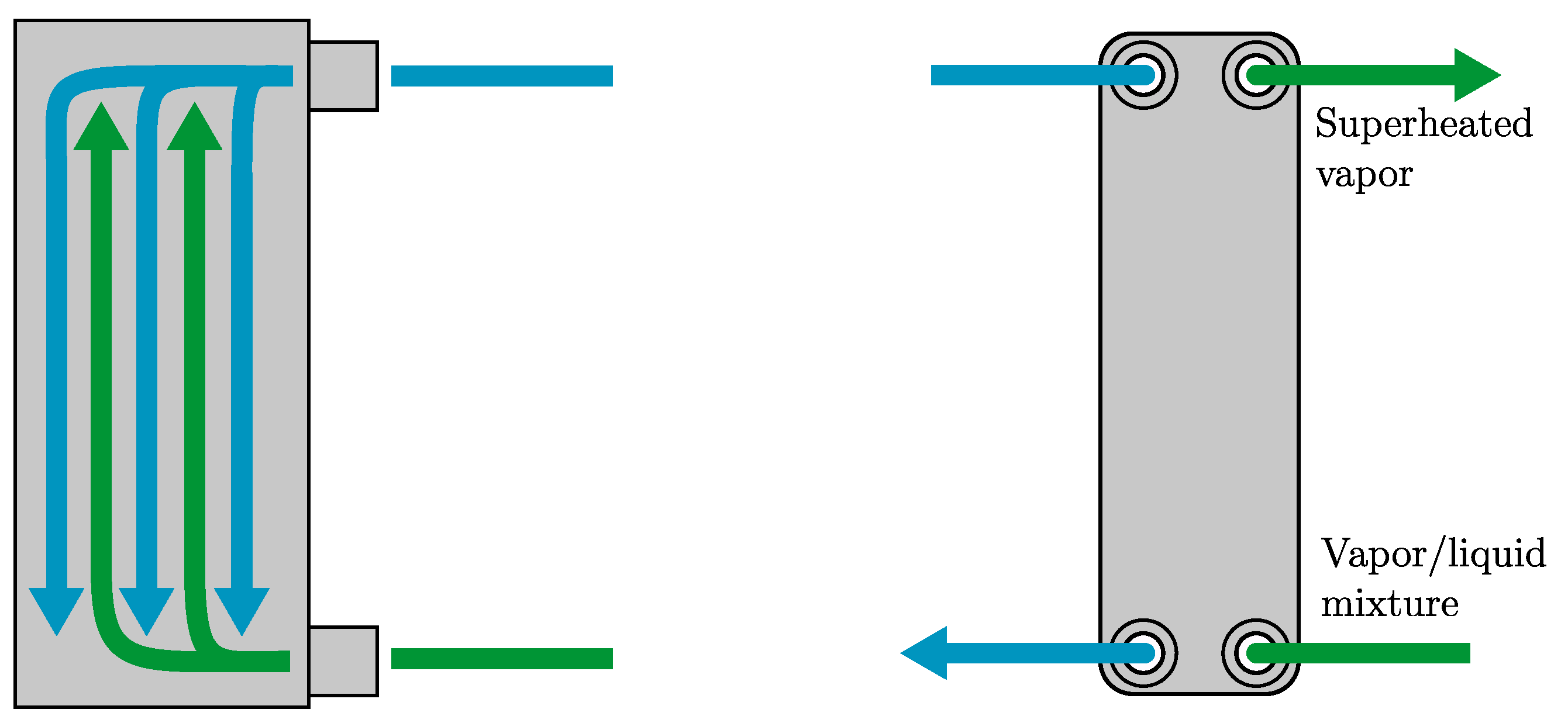
The most common automotive heat exchanger for refrigerant-to-coolant applications is the brazed plate heat exchanger, whose working method as a counter-flow chiller is shown in Figure 2. At the refrigerant inlet, the fluid is typically in a vapor–liquid mixture and evaporates as it flows through the heat exchanger, maintaining its pressure-dependent saturation temperature until the fluid is one hundred percent gas. While the temperature remains constant, the local heat transfer rate is strongly dependent on the local vapor fraction, which varies across the length of the device.

An extension of the system in Figure 1 is shown in Figure 3. If the ambient temperatures are normally lower than the battery temperature setpoint, an additional radiator ($Q_5$) can be added to the system.

Modern vehicles are equipped with air-conditioning systems for cabin cooling. To avoid having two separate refrigeration cycles running independently, the systems are combined, typically as shown in Figure 4, where the battery chiller ($Q_2$) and the cabin evaporator ($Q_6$) both share the external condenser ($Q_4$). The expansion valves ($X_1$ and $X_2$) control the flow through their respective heat exchangers. Heating for this system is accomplished by the electric battery heater ($Q_1$).

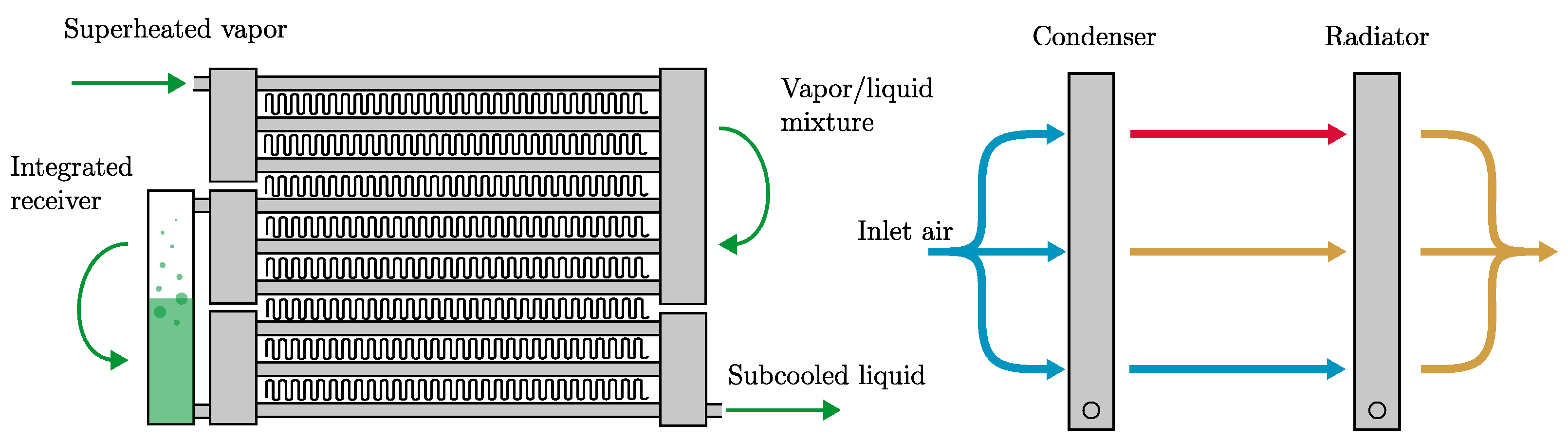
An air-to-refrigerant heat exchanger working as a condenser is shown in Figure 5. Condensers are typically constructed of multiple passes. Each pass consists of a number of tubes interleaved with finned sheet plating. Each tube is perforated with several minichannels to increase the effective heat transfer area to the refrigerant.

It is common to include an integrated receiver between the last two passes of the condenser (second and third as shown in Figure 5). The receiver serves three functions in automotive refrigerant systems. The first is to act as a storage device for the liquid refrigerant when the system is not operating. Secondly, the receiver vessel typically contains a desiccant material that absorbs moisture, protecting the components from damage. Thirdly, following the discussion in [63], while the system is operating, the receiver acts as a buffer vessel, ensuring that only liquid refrigerant reaches the expansion valve ($X_1$): the level of stored liquid in the receiver increases or decreases depending on the thermodynamic state at the condenser outlet. Since the receiver volume is large enough to ensure that the refrigerant it contains always exists in a saturated state, only saturated liquid will leave the vessel. For example, if a vapor–liquid mixture enters the receiver, its enthalpy will increase and cause the stored liquid to evaporate. A greater portion of the refrigerant existing in a gaseous phase results in higher system pressures, which increase the saturation temperature of the condenser and consequently increase the heat transfer from the refrigerant. The pressure continues to rise until the refrigerant at the condenser outlet is a saturated liquid, whereupon a steady state is achieved.

Figure 6 shows the first method of improving the efficiency of cabin and battery heating through reducing the dependence on the electric heater ($Q_1$). A heat pump is technically nothing more than a reversed refrigeration cycle, which is realized by introducing the four-way reversing valve ($V_3$). $V_3$ enables the refrigerant to flow in reverse direction, turning the battery chiller ($Q_2$) and the cabin evaporator ($Q_6$) into condensers and the external condenser ($Q_4$) into an evaporator. Of course, additional shut-off valves ($V_4$, $V_5$, and $V_6$) are necessary. The cooling mode is achieved by setting the reversing valve as indicated in the figure, while $V_4$ is left open, $V_5$ is closed, and $V_6$ is open. Thus, the system simplifies to that shown in Figure 1. The heating mode is achieved by turning $V_3$ such that a clockwise flow direction follows, where $V_5$ is opened and $V_4$ is closed. $V_6$ may be open or closed, depending on the need for battery cooling. In this configuration, the net effect is a transfer of heat from the low ambient temperature to the cabin compartment and the battery coolant loop, at the price of compression work. In the heating mode, the evaporator ($Q_4$) pressure is dependent on the ambient temperature. For very low ambient temperatures, an equally low pressure must be maintained in the evaporator, at greater cost in terms of compression work.

Thus, further efficiency gains can be achieved by harvesting waste heat from the motor and power electronics systems. One possible realization of this technology is shown in Figure 7. The system in Figure 6 is extended with a motor chiller ($Q_7$), whose purpose is to cool the medium temperature (MT) loop, thereby transferring heat to the refrigerant. This heat is then available for either the cabin condenser ($Q_6$) or the battery loop condenser ($Q_2$). As opposed to the system in Figure 6, the evaporator pressure for the waste-heat recovery system in Figure 7 is not as dependent on the ambient temperature.

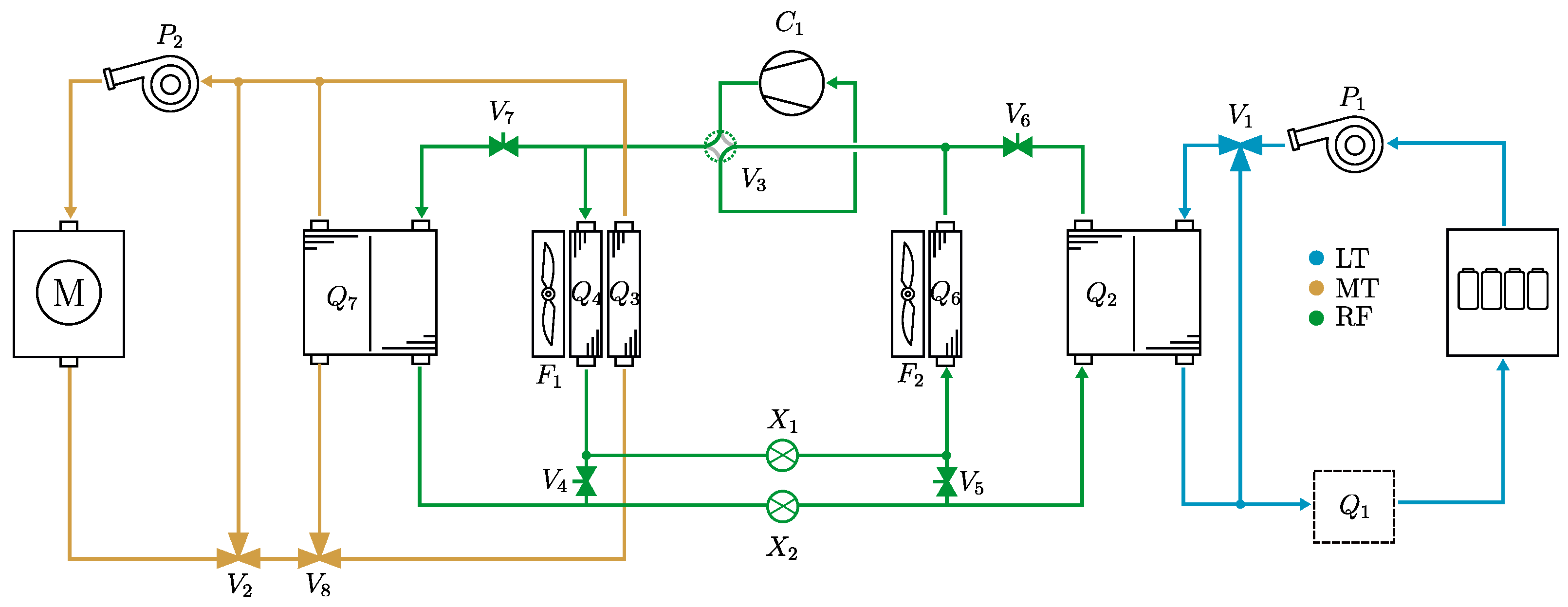
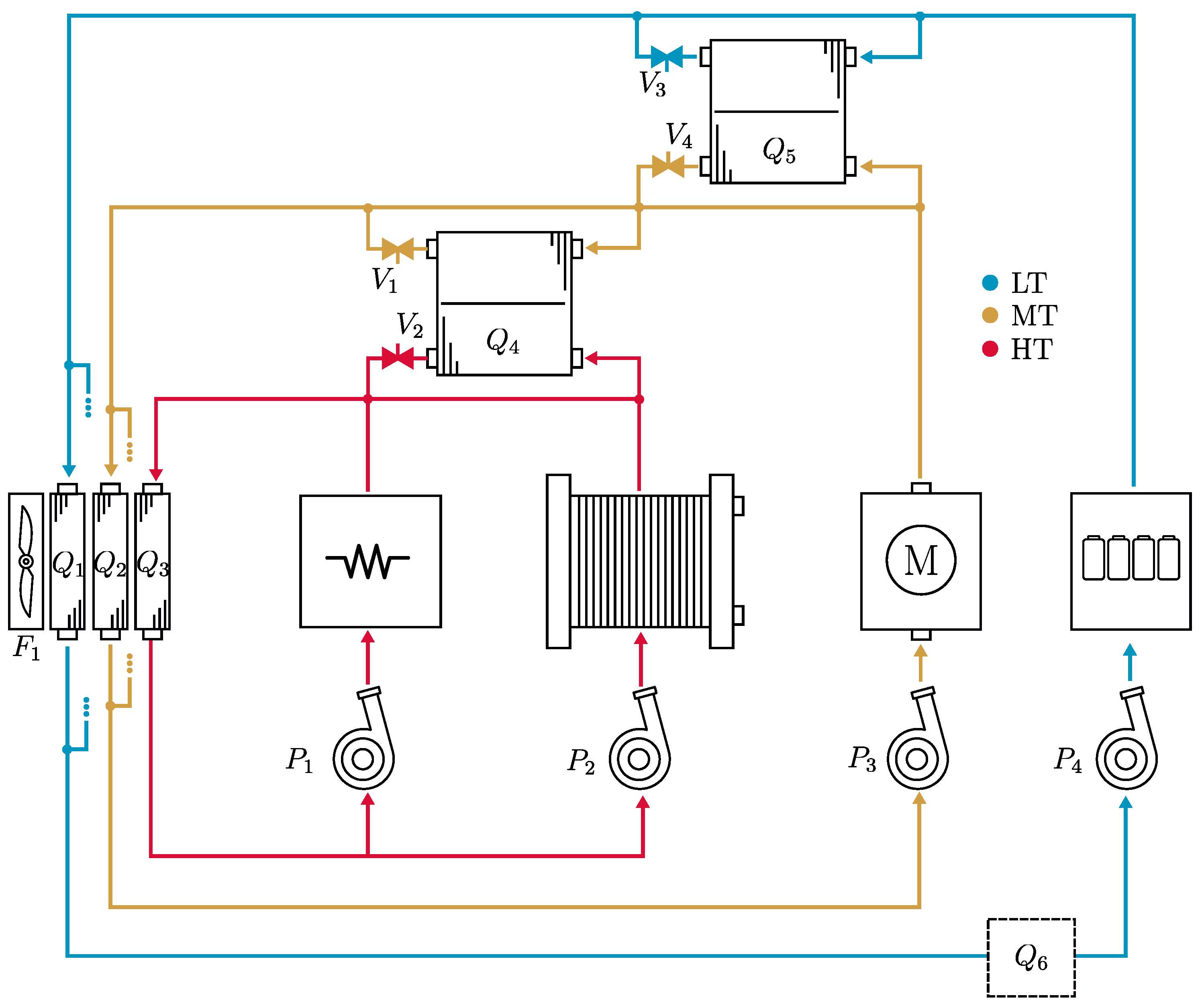
Thermal management systems for fuel cell hybrid powertrains employ additional radiators to deal with the overheating problem. Figure 8 shows a system with (from left to right) a front-mounted fan ($F_1$) and radiator ($Q_1$) assembly, a brake resistor, two separate fuel cell stacks, and two additional fan and radiator assemblies ($F_2$ and $Q_2$, $F_3$ and $Q_3$) mounted on the sides of the truck. The radiator bypass valve ($V_1$) is responsible for regulating the high-temperature (HT) coolant loop, while the secondary valve ($V_2$) can be opened if additional cooling power is required.

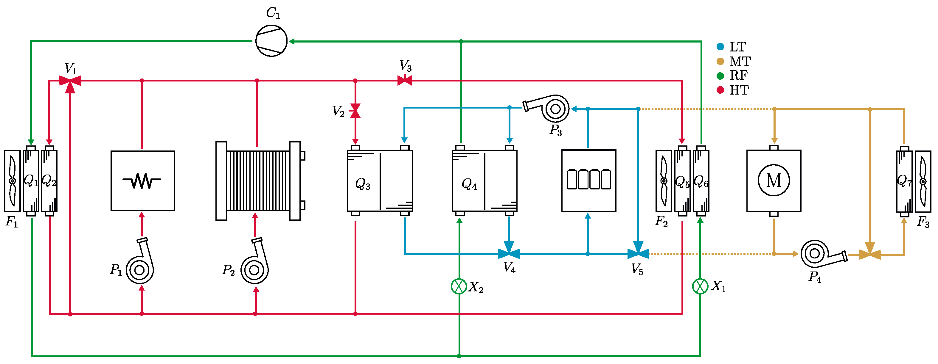
Waste-heat recovery can be achieved in multiple ways for the fuel cell hybrid systems. As shown in Figure 9, three fluidically separate but thermally connected loops are used, each with their own dedicated front-mounted radiator ($Q_1$, $Q_2$, and $Q_3$). By actuating the valves ($V_1$, $V_2$, $V_3$, and $V_4$) waste-heat from the fuel cell stacks and motor can be transferred to the battery loop. Of course, lacking a refrigeration system, this design will suffer in high-temperature environments.

A state-of-the-art TMS designed for fuel cell hybrid trucks is shown in Figure 10. Here, four fluid circuits are used to manage the thermal states of the vehicle. The high-temperature (HT) circuit cools the fuel cell stack and brake resistor, while also providing waste heat to the battery loop through a liquid-to-liquid heat exchanger ($Q_3$), and the cabin compartment through a heater core ($Q_5$). The refrigeration cycle is used to cool the cabin compartment through the evaporator ($Q_6$) and the battery loop through a chiller ($Q_4$). A heat pump is not necessary since the fuel cell stack produces sufficient waste heat for the cabin and battery. The motor and power electronics are cooled by a medium temperature (MT) loop through a side-mounted radiator ($Q_7$).

The cabin air flow system is also an important part of thermal management. The cabin air is maintained at a temperature setpoint through various methods shown in the schematics thus far. It is also necessary to circulate air through the cabin to keep it fresh and limit humidity. Therefore, an air flow control system manages the air flow through fans/blowers and flaps, as shown in Figure 11. The first and third flaps ($V_1$ and $V_3$) and the blower ($F_1$) regulate the net air intake to a desired level. The second flap ($V_2$) controls the air flow through the heating or cooling devices ($Q_1$ and $Q_2$) and thus regulates the cabin temperature. To keep the cabin air fresh, a minimum net flowthrough is required, which can be a significant load on the cabin air conditioning systems. To limit the air conditioning load in these cases, the net air intake is reduced to its minimum level, and a recirculation fan ($F_2$) is used to achieve the sufficient level of air flow required for good heat transfer conditions in the cabin-mounted heat exchangers ($Q_1$ and $Q_2$).

Thermal Management System Control

As shown in the previous section, the thermal management architectures of modern electric vehicles have become complex interconnected systems with multiple competing objectives and actuators. It follows that designing control algorithms for these systems have also become more difficult; however, the difficulty has not only come from the additional control objectives and actuators. There has also been a shift in viewpoint with respect to thermal management.

Traditionally, the thermal management problem has consisted of moving heat from one principal component, the combustion engine, to the ambient environment and if needed, the cabin compartment. This viewpoint is shown on the left in Figure 12. In contrast, the modern viewpoint of TMSs for electric vehicles is to view the vehicle components as both consumers and producers of heat, and the TMS the network in which transactions occur, as shown on the right in Figure 12. This viewpoint requires the online solution of network optimization problems that aim to satisfy each component’s need of heating or cooling.

In addition to solving the steady-state heat distribution problem posed in Figure 12, modern predictive energy management strategies to a greater extent consider the thermal states of the vehicle, in what is commonly referred to as combined energy and thermal management. Typically, only mechanical and electrochemical states such as velocity and state of charge have been included in onboard mission planning.

3. Modeling

Following the schematics in Figure 1, Figure 2, Figure 3, Figure 4, Figure 5, Figure 6, Figure 7, Figure 8, Figure 9, Figure 10 and Figure 11, the scope of the modeling work becomes clear. First, three types of fluids need to be modeled: air, coolant, and refrigerant. The fluids should act as a medium for heat transfer between the vehicle components. Further, models for junctions (splits and convergences in the flow path) are needed for all three fluids. They also need to be implemented in a way that is thermodynamically valid. While air and coolant may be treated as a single-phase medium, the refrigerant circuit requires the consideration of phase changes and thus a significantly more detailed treatment. In addition to the fluid medium properties, several other components are required, namely the heat exchangers, pumps, fans, valves, and pipes that construct the TMS, as well as the thermal models for the battery, fuel cell, motor, power electronics, and cabin compartment. A nomenclature for the equations and formulas to follow is shown in Nomenclature.

3.1. Air, Coolant, and Refrigerant Flow Circuits

The coolant medium and its thermophysical properties was a 50% water–ethylene glycol mixture with a constant density, thermal capacity, and thermal conductivity, taken from CoolProp (version 6.6.0) [64], and evaluated at $T=60$ °C, while air parameters were evaluated at $T=25$ °C and atmospheric pressure. The thermophysical properties of the refrigerant are considered in a separate section in the following.

An approach to flow modeling was adopted where pressure information was fed back from merging to diverging junctions, where a ratio was calculated to ensure that pressures in the merging junction converged in a steady state. The rate at which the pressures converged was a tuneable parameter, and its value depended on the trade-off between computational speed and the impact of transient condition errors. For driving missions where the TMS operates in a steady state for most of the mission’s duration, a convergence rate in the order of seconds provides a good balance between numerical stability and accuracy.

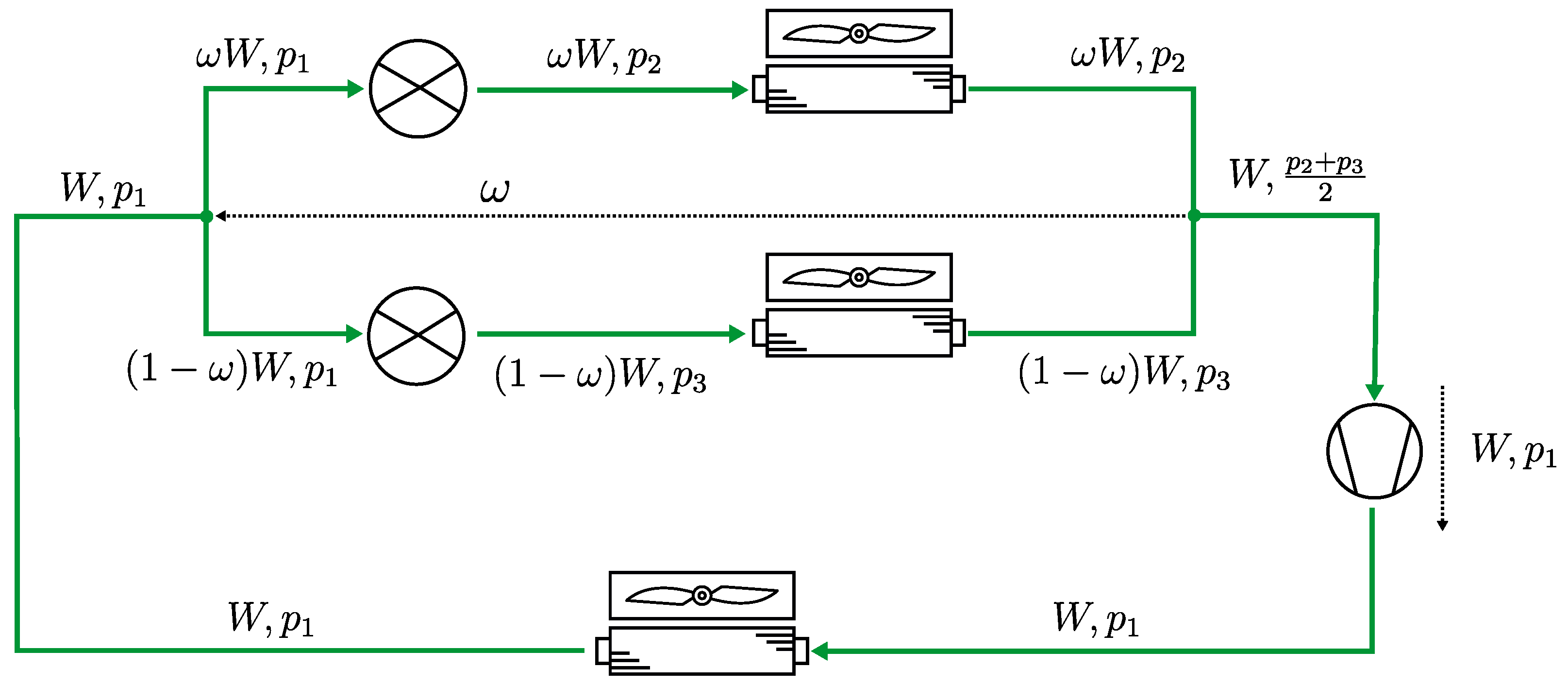
The flow–pressure balancing method is shown in Figure 13, Figure 14 and Figure 15. The output of the loop’s flow-balancing component was the total flow W and pressure $p_1$. At the first junction, the flow distributed on the two branches according to the ratio $\omega$, and on each branch, the pressure was increased from $p_1$ to $p_2$ and $p_3$ by a coolant pump. The flows merged in the second junction, and the pressure was assumed to be the mean value of the incoming branches. The flow split ratio,

$$\begin{array}{c}\hfill \dot{\omega }=\gamma (p_2-p_3),\end{array}$$

was calculated by integrating a first-order system that depended on the merging branch pressure difference and a gain parameter $\gamma$. That is, if $p_2>p_3$ then $\omega$ would increase, in turn increasing the flow through branch one. A higher flow resulted in a reduced pressure head according to the pump curve, which would cause $p_2$ to drop, and inversely, $p_3$ to rise until $p_2=p_3$. The temperature output of the merging junction was calculated according to the mass flow ratio and temperatures of the incoming streams.

Similar to the flow split ratio, the total flow (W) in the circuit was given by the differential equation

$$\begin{array}{c}\hfill \dot{W}=\beta \left(p_1-{\displaystyle \frac{p_2+p_3}{2}}\right).\end{array}$$

That is, the total circuit flow W was determined by the difference in pressure over the flow-balancing component. $\beta$ was a tuneable parameter similar to $\gamma$.

Commonly, a radiator is often in part covered by a condenser, which is the scenario shown in Figure 14. Thus, the covered radiator is split in two parts, one covered and one exposed. The air stream splits before the heat exchanger as shown in the figure and then merges afterwards before the fan. This splitting and merging of the flow path was treated in the same way as for the coolant system discussed above.

The refrigerant circuit flow modeling was treated similarly to the coolant and air circuits, the main difference being that the flow W was given by the compressor model (calculated from the compressor speed and pressure ratio) and propagated through the system. The high-side pressure $p_1$ was a parameter chosen by the user, a simplification made to avoid dealing with refrigerant charge. The receiver pressure modulation can be included through a control system which regulates the high-side pressure such that the receiver inlet stream is saturated liquid.

Compared to methods discussed in, for example, Ref. [65], the strategy to model coolant flows for the ECCV platform cannot handle reversing flows, but the benefits are instead the simplicity and computational speed. With the adopted methodology, the flow–temperature–pressure information propagates downstream, except in junctions, where the flow distribution ratio $\omega$ is fed from the point of convergence back to the splitting junction.

3.2. Refrigerant Thermodynamics

Due to global warming potential and flammability restrictions placed on automotive refrigerants, R1234yf emerged in the 2020s as the main contender to replace R134a and is used in most EVs in production. Its foremost competitors are R290 (propane), which has an exceptionally low global warming potential but is highly flammable, and R744 (carbon-dioxide), which requires extremely high pressures and is commonly seen in application with high air conditioning loads such as buses. In this work, R1234yf was chosen as the refrigerant, but the methods described in this section are also applicable to similar refrigerant fluids.

Refrigerant flow is more complex to model than single-phase systems. For coolant flow, temperature and pressure are a natural choice of propagation variables, while for a two-phase flow, temperature and pressure are insufficient to fully specify the thermodynamic state. In this work, pressure and specific enthalpy were used, as they are the default pair of thermodynamic variables considered in most commercial refrigerant flow modeling software.

The pressure and flow balancing of the refrigerant system were modeled exactly like the coolant circuit. The fluid was considered to be incompressible, even in the gas phase, and components such as compressors, expansion valves, and refrigerant lines functioned as pressure boosters or pressure drops, where the split and merge components governed the equalizing of pressures and diverting of flow.

Refrigerant system component models require the calculation of other thermodynamic variables than pressure and enthalpy, which necessitates an equation of state. Multiparameter equations of state are mathematical models that relate thermodynamic state variables with extreme accuracy, and although the equations are typically explicit in the Helmholtz energy as a function of density and temperature, a convenient feature of the multiparameter state equations is that all other thermodynamic state variables can be accessed through particular combinations of partial derivatives. The general equations shown below and the lists of partial derivative combinations used in this work are found in [66].

In addition to the equation of state, other thermophysical properties like the surface tension and thermal conductivity are required, and the source of their correlations are presented in

Table 1. Thermophysical properties references.

Property	Reference
Equations of state	[67]
Speed of sound	[68]
Surface tension	[69]
Thermal conductivity	[70]
Viscosity	[71]
Saturation correlations	[72,73]

. The equations and correlations references was provided by the CoolProp [64] documentation.

If temperature and density are known, all other thermodynamic state variables can be calculated through a combination of partial derivatives of the Helmholtz energy. For a circuit where pressure and enthalpy are the variables communicated between components, neither temperature nor density are known, and therefore need to be calculated. The procedure for calculating a thermodynamic state variable using two others is called a “flash” calculation, and the numerical difficulty of this procedure varies depending on which variables are known, and which are sought. For the refrigerant flow case, pressure and enthalpy are known, so temperature and density need to be solved simultaneously. This is a time-consuming operation and not feasible to perform during simulation. Instead, 2D lookup tables were generated to find temperature and density from a known pressure and enthalpy.

To generate pressure–enthalpy (p-h) lookup maps, the equations that need to be solved are

$$\begin{array}{c}\hfill p=p(\rho ,T),h=h(\rho ,T),\end{array}$$

(1)

in the single-phase region, where $\rho$ and T are the fluid density and temperature, and

$$\begin{array}{c}\hfill p=p_v\left(T\right)=p_f\left(T\right),h=x{h}_v\left(T\right)+(1-x)h_f\left(T\right),\end{array}$$

in the two-phase region, where x is the vapor fraction, and the subscripts f and v denote the saturated vapor and liquid properties for the given temperature T. Therefore, before generating the map, the phase envelope needs to be accurately outlined. For vapor–liquid equilibrium, with g denoting the Gibbs energy, it holds that

$$\begin{array}{c}\hfill g_v=g_f,p_v=p_f,T_v=T_f,\end{array}$$

so the equations

$$\begin{array}{c}\hfill g({\rho }_f,T)=g({\rho }_v,T),p({\rho }_f,T)=p({\rho }_v,T)\end{array}$$

(2)

may for a known temperature be solved to find the two solutions corresponding to the saturated vapor and liquid phase densities, ${\rho }_v$ and ${\rho }_f$, by using the critical density ${\rho }_c$ as lower and upper bounds according to the inequality

$$\begin{array}{c}\hfill {\rho }_v<{\rho }_c<{\rho }_f.\end{array}$$

A numerical solution to Equation (2) is shown in Figure 16 and compared to single-phase pressure-volume-temperature ($p\text{-}v\text{-}T$) data from [67].

With the saturation densities known, any other saturation variable can be calculated using the partial derivatives of the state equation,

$$\begin{array}{c}\hfill h_v=h({\rho }_v,T),h_f=h({\rho }_f,T),p_v=p({\rho }_v,T),p_f=p({\rho }_f,T)\end{array}$$

so any given pressure and enthalpy can be compared against the saturation curves to determine the active phase region, and the correct equations to use when solving for $\rho$ and T.

Nonlinear equation solvers need an initial guess for density and temperature. A cubic equation of state like the Peng–Robinson [74] equation can be used to find an initial guess $T_0$ and ${\rho }_0$ with the equations

$$\begin{array}{c}\hfill p=p({\rho }_0,T_0),h=h({\rho }_0,T_0),{\rho }_0={\rho }_{PR}(p,T_0).\end{array}$$

The results for the initial step of finding the phase envelope, as compared to p-v-T data from [67] is shown in Figure 16, along with the temperature lookup map generated by the solution of Equation (1).

3.2.1. Pipe and Channel Models

The pressure drop for the pipe and channel flow was calculated using the Darcy–Weisbach friction factor ($f_D$) correlations [75]

$$\begin{array}{cc}\hfill f_{D,\mathrm{lam}}& ={\displaystyle \frac{64}{\mathrm{Re}}},{\displaystyle \frac{1}{\sqrt{f_{D,\mathrm{turb}}}}}=-1.8{log}_{10}\left[{\displaystyle \frac{6.9}{\mathrm{Re}}}+{\left({\displaystyle \frac{ϵ/D}{3.7}}\right)}^{1.11}\right]\hfill \\ \hfill f_D& =y{f}_{D,\mathrm{turb}}+(1-y)f_{D,\mathrm{lam}},y=0.5tanh\left({\displaystyle \frac{\mathrm{Re}-2100}{100}}\right)+0.5\hfill \end{array}$$

where D is the hydraulic diameter of the pipe, Re the fluid Reynolds number, and the subscripts lam and turb denote the laminar and turbulent regions. A hyperbolic tangent function was used, through the variable y, for a smooth transition from laminar to turbulent flow, as shown in the left of Figure 17. In addition to a pressure drop, the pipe model also included a variable time delay for the coolant temperature, which depended on the pipe length and flow speed.

The Hausen and Sieder–Tate correlations for the Nusselt number (Nu) [76],

$$\begin{array}{cc}\hfill {\mathrm{Nu}}_{\mathrm{lam}}& =3.66+{\displaystyle \frac{0.0668\mathrm{Re}\mathrm{Pr}(D/L)}{1+0.04{\left(\mathrm{Re}\mathrm{Pr}\right)}^{2/3}}},{\mathrm{Nu}}_{\mathrm{turb}}=0.027{\mathrm{Re}}^{4/5}{\mathrm{Pr}}^{1/3}\hfill \\ \hfill \mathrm{Nu}& =y{\mathrm{Nu}}_{\mathrm{turb}}+(1-y){\mathrm{Nu}}_{\mathrm{lam}},y=0.5tanh\left({\displaystyle \frac{\mathrm{Re}-3500}{400}}\right)+0.5\hfill \end{array}$$

were used to model convective heat transfer in laminar and turbulent channel flows, where Pr is the fluid Prandtl number. The Nusselt number as a function of the Reynolds number is shown to the right in Figure 17.

3.2.2. Restrictions

For the system in Figure 13, the amount of flow distributed on each branch can be controlled by varying the pump speeds. Faster pump speeds produce higher discharge pressures and therefore, more flow is required to balance the pressures at the merging point. Flow (W) can also be controlled in a similar manner using pressure drops from flow restrictions ($\Delta p$), which was implemented in the platform using the Bernoulli’s obstruction equation [77]

$$\begin{array}{c}\hfill \Delta p=(1/2\rho )(1-{\beta }^4){\left({\displaystyle \frac{W}{C_{d}A}}\right)}^2,\beta =d/D\end{array}$$

where common flow restriction-based components were modeled by manipulating the pipe and orifice area, D and d.

3.3. Pumps and Fans

Two electric water pumps, the WP120 and WP150 from EMP [78], and one fan, the VA164A from SPAL [79], were included in the ECCV platform. The water pumps were modeled by correlating flow, pressure, speed, and power consumption data as simple polynomials and the fan affinity laws, where the model fit to data is shown in Figure 18, Figure 19 and Figure 20.

3.4. Two-Phase Flow in Pipes

Two-phase flow pressure drop was calculated using first the correlation developed in [80] for single-phase-only friction factors ($f_{\mathrm{lo}}$)

$$\begin{array}{cc}\hfill f_{\mathrm{lo}}& =0.25{\left[{log}_{10}\left({\displaystyle \frac{150.39}{{\mathrm{Re}}_{\mathrm{lo}}^{0.98865}}}-{\displaystyle \frac{152.66}{{\mathrm{Re}}_{\mathrm{lo}}}}\right)\right]}^{-2},{\mathrm{Re}}_{\mathrm{lo}}={\displaystyle \frac{G_{\mathrm{tp}}D}{{\mu }_l}},\hfill \end{array}$$

i.e., a friction factor correlated to a Reynolds number calculated using the liquid only (lo) or gas only (go) single-phase dynamic viscosity ${\mu }_l$ or ${\mu }_g$ and the two-phase mass flux $G_{\mathrm{tp}}$. The two-phase pressure gradient ${(\partial p/\partial z)}_{tp}$ was then calculated by multiplying the liquid-only pressure gradient

$$\begin{array}{c}\hfill {\left({\displaystyle \frac{\partial p}{\partial z}}\right)}_{\mathrm{lo}}=f_{\mathrm{lo}}{\displaystyle \frac{G_{\mathrm{tp}}^2}{2D{\rho }_l}},\end{array}$$

with a two-phase multiplier ${\varphi }_{\mathrm{lo}}$ given by the correlation in [81]:

$$\begin{array}{cc}\hfill Y& =\sqrt{{(\partial p/\partial z)}_{\mathrm{go}}/{(\partial p/\partial z)}_{\mathrm{lo}}}\hfill \\ \hfill {\varphi }_{\mathrm{lo}}& =\left(Y^2{x}^3+{(1-x)}^{1/3}[1+2x(Y^2-1)]\right)\left[1+1.54{(1-x)}^{0.5}{\mathrm{La}}^{1.47}\right],\hfill \end{array}$$

where La is the fluid Laplace number.

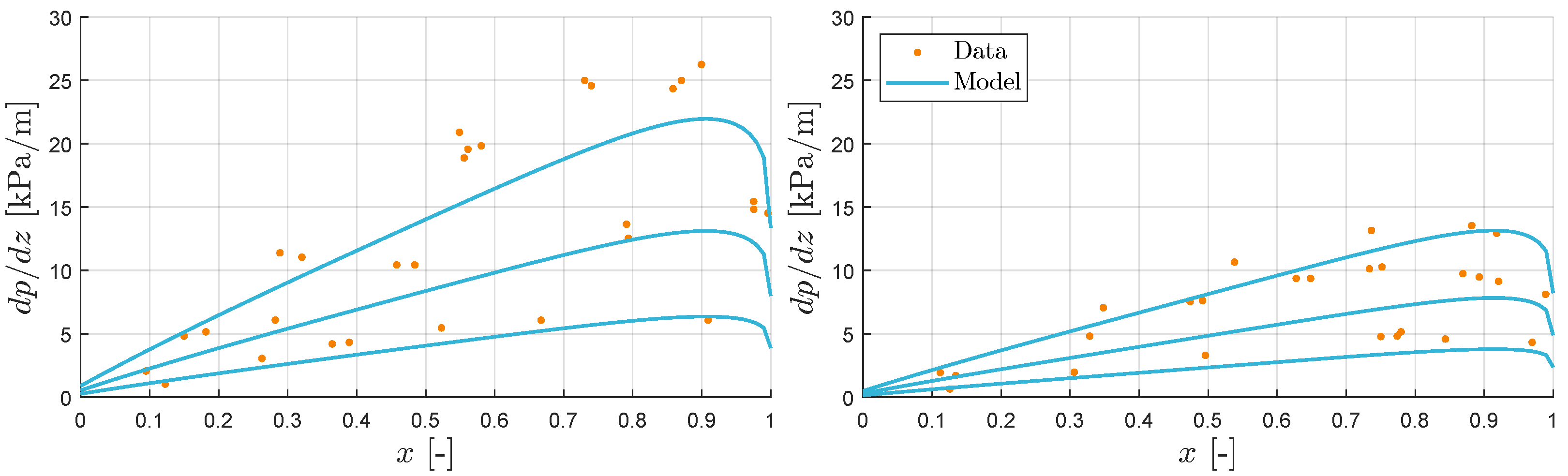
The pressure gradient was compared to data from [82] and is shown in Figure 21 for mass fluxes $G_{\mathrm{tp}}=200$, 300 and 400 [kg/s m²] and pipe diameters $D=3.2$ mm and 4.8 mm.

Similarly to coolant pipes, a variable time delay was applied to the specific enthalpy to capture the dynamic effects and transport in long pipes.

3.5. Refrigerant Compressor

The compressor model was taken from [83], where the author parameterized the model to multiple compressor types and datasets and found good results. One of the datasets was taken from [84], a reciprocating compressor designed for automotive air conditioning, and was included in the ECCV platform. First, correlations for a reference suction-line volumetric flow (${\dot{V}}_{\mathrm{ref}}$) and reference electric power consumption ($P_{\mathrm{ref}}$) were parameterized to the data at a single reference speed $N_{\mathrm{ref}}$,

$$\begin{array}{c}\hfill {\dot{V}}_{\mathrm{ref}}=\left[b_1+b_2{\left({\displaystyle \frac{p_d}{p_s}}\right)}^{1/\kappa }\right]N_{\mathrm{ref}}{V}_{\mathrm{disp}},P_{\mathrm{ref}}=p_s{\dot{V}}_{\mathrm{ref}}{a}_1\left[{\left({\displaystyle \frac{p_d}{p_s}}\right)}^{a_2+(\kappa -1)/\kappa }+{\displaystyle \frac{a_3}{p_d}}\right]+P_{\mathrm{loss}}\end{array}$$

Normalized volumetric and isentropic efficiencies, (${\eta }_v/{\eta }_{v,\mathrm{ref}}$) and (${\eta }_{is,\mathrm{ref}}/{\eta }_{is}$) were then correlated to the normalized speed ($N/N_{\mathrm{ref}}$) through the parameters d and e as

$$\begin{array}{c}\hfill {\displaystyle \frac{{\eta }_v}{{\eta }_{v,\mathrm{ref}}}}=d_1+d_2\left({\displaystyle \frac{N}{N_{\mathrm{ref}}}}\right)+d_3{\left({\displaystyle \frac{N}{N_{\mathrm{ref}}}}\right)}^2,{\displaystyle \frac{{\eta }_{is,\mathrm{ref}}}{{\eta }_{is}}}=e_1+e_2\left({\displaystyle \frac{N}{N_{\mathrm{ref}}}}\right)+e_3{\left({\displaystyle \frac{N}{N_{\mathrm{ref}}}}\right)}^2,\end{array}$$

which then allowed the computation of flow rate $\dot{V}$ and power consumption P at any speed as

$$\begin{array}{c}\hfill \dot{V}={\dot{V}}_{\mathrm{ref}}\left({\displaystyle \frac{N}{N_{\mathrm{ref}}}}\right)\left({\displaystyle \frac{{\eta }_v}{{\eta }_{v,\mathrm{ref}}}}\right),P=P_{\mathrm{ref}}\left({\displaystyle \frac{\dot{V}}{{\dot{V}}_{\mathrm{ref}}}}\right)\left({\displaystyle \frac{{\eta }_{is,\mathrm{ref}}}{{\eta }_{is}}}\right).\end{array}$$

The dataset in [84] and parameter fit by [83] used R134a as the refrigerant. Using R1234yf instead gave a small constant error in flow and power consumption for all data points which could be removed by decreasing the suction line density by ten percent and increasing the compressor electrical losses from 350 W to 700 W. The resulting model fit is shown in Figure 22.

3.6. Heat Exchangers

Four types of heat exchangers were considered in this work: air-to-coolant, air-to-refrigerant, coolant-to-refrigerant, and coolant-to-coolant.

The air-to-coolant heat exchanger model was based on the effectiveness-NTU method, where the overall heat transfer coefficient U was correlated to the air and coolant stream velocities as

$$\begin{array}{c}\hfill 1/U=a_1+a_2{v}_{\mathrm{air}}^{a_3}+a_4{v}_{\mathrm{cl}}^{a_5}\end{array}$$

where the parameter set $a_1\cdots a_5$ corresponds to four possible choices of radiator depth, ranging from 19 to 52 mm. The parameter set and heat exchanger model structure used in this work was developed by collaborators at TitanX AB, Sölvesborg, Sweden. The effectiveness ($ϵ$) correlation for unmixed cross-flow conditions was given by [76] as

$$\begin{array}{c}\hfill ϵ=1-exp\left[{\displaystyle \frac{exp(-NCn)-1}{Cn}}\right],C={\displaystyle \frac{C_{\min }}{C_{\max }}},n=N^{-0.22}\end{array}$$

where C is the ratio of heat capacity rates, and $N=UA/C_{\min }$ the number of transfer units.

The coolant-to-refrigerant heat exchanger was implemented as the brazed plate heat exchanger in Figure 2. The refrigerant side heat transfer coefficient is strongly dependent on the local vapor fraction, which varies over the length of the refrigerant flow path inside the device. The heat exchangers were initially modeled using a discretized grid approach, so that the effect of a varying vapor fraction was captured. However, when the discretized model was compared to a much simpler implementation where only the coolant side single-phase heat transfer coefficient was considered, it was found that both models gave similar predictions. The simpler model was adopted for the platform. With G denoting the coolant mass flux, and $c_p$ its specific heat capacity, the single-phase coolant side heat transfer coefficient (h) correlation was given by

$$\begin{array}{c}\hfill h=0.494G{c}_p{\mathrm{Re}}^{-0.426}{\mathrm{Pr}}^{-2/3},\end{array}$$

a correlation developed in [85], where the authors performed experiments on counterflow offset strip fin brazed plate heat exchangers.

A similar method was used to model the air-to-refrigerant heat exchangers. The discretized grid model performed similarly to a much simpler approach using only the single-phase heat transfer coefficient on the air side. The air-to-refrigerant heat exchanger was implemented as a louvered-fin cross-flow radiator, shown in Figure 5. With u denoting the free stream velocity of the radiator air flow, together with A and $A_{\min }$ denoting the total and minimum flow area as seen in the flow direction, the air side heat transfer coefficient was calculated using the Colburn j-factor from [86] as

$$\begin{array}{c}\hfill h=j\rho u\sigma (c_p/{\mathrm{Pr}}^{2/3}),\sigma =A/A_{\min },\end{array}$$

where j, given by

$$\begin{array}{cc}\hfill j& ={\mathrm{Re}}^{-0.487}{(L_a/90)}^{0.257}{(F_p/L_p)}^{-0.13}{(H/L_p)}^{-0.29}\dots \hfill \\ \hfill & \dots {(F_d/L_p)}^{-0.235}{(L_l/L_p)}^{0.68}{(T_p/L_p)}^{-0.279}{(d_f/L_p)}^{-0.05},\hfill \end{array}$$

is a correlation of the Reynolds number and ratios of louvered-fin dimensions specified in

Table 2. Louvered-fin geometry.

Dimension	Symbol	Unit
Louver angle	$L_a$	°
Louver pitch	$L_p$	m
Louver length	$L_l$	m
Fin pitch	$F_p$	m
Fin height	H	m
Fin thickness	$d_f$	m
Tube pitch	$T_p$	m
Flow depth	$F_d$	m

. See [86] for a detailed description of the louvered-fin geometry.

3.7. Thermal Inertia

Two methods were included to model component temperatures. The first method applied to components whose thermal inertia was insignificant, where the component temperature may be sufficiently approximated as equal to the outlet coolant temperature. In such cases, the heat produced by the component was simply added to the coolant, and a temperature increase followed. For components with large thermal inertias such as the fuel cell stacks and battery pack, the temperature was modeled dynamically as a balance of its generated heat $Q_{\mathrm{gen}}$ and the applied cooling power, where the dynamic response time was a function of the component mass m and its specific heat as

$$\begin{array}{cc}\hfill m{c}_p\dot{T}& =Q_{\mathrm{gen}}-Q_{\mathrm{cool}}.\hfill \end{array}$$

The generated heat $Q_{\mathrm{gen}}$ and cooling power $Q_{\mathrm{cool}}$ were calculated from the component loss models and the channel heat transfer correlations described above.

3.8. Simulink Implementation

The sections above complete the necessary component models to build the systems shown in the schematics (Figure 1, Figure 2, Figure 3, Figure 4, Figure 5, Figure 6, Figure 7, Figure 8, Figure 9, Figure 10 and Figure 11). The models were implemented in the ECCV Simulink framework discussed further in [20]. An example of using the component models in Simulink is shown in Figure 23, where the simple system in Figure 13 was implemented. The coolant properties (temperature, pressure, and flow) were propagated through the models in vector format. In addition to the inlet coolant conditions, the pump models took as inputs a voltage and a desired speed. A pressure boost was calculated according to the pump models described above, and the output coolant state was output to the next component models. Figure 23 shows a simple example, but with this modular approach, large and complex coolant and refrigerant networks can be built.

4. Results and Discussion

Two challenging thermal management scenarios were investigated as case studies. As cold climates are considered the main challenge for battery electric vehicles, the first scenario considers the potential driving range improvements of the air-source heat pump shown in Figure 6 and the waste-heat recovery system shown in Figure 7, compared to pure electric heating for ambient temperatures down to −15 °C.

The second scenario considered the potential cooling capacity gains by including a side-mounted radiator for fuel cell hybrid vehicles operating in high ambient temperature environments. The system shown in Figure 10 was used as a baseline and was extended with an additional radiator as shown in Figure 8. The objective of the scenario was then to determine the maximum possible ambient temperature for each system when maintaining a stack temperature of 80 °C.

Both scenarios were evaluated for a truck weight of 20 and 40 tons.

4.1. Vehicle and Power Control

The control system was simple and used only single input–single output proportional–integral (PI) regulators to satisfy the mission objectives. The velocity target was 80 km/h and maintained by adjusting the torque demand on the electric motors. For the battery electric vehicle, the DC bus was maintained at seven hundred volts by adjusting the battery current only, while for the fuel cell hybrid, the bus was regulated by a combination of power sources, whose ratio of contribution was determined by the operating conditions. If the battery was charging at maximum capacity (a situation that might occur when driving downhill) the fuel cell stack output was temporarily reduced to allow maximum recuperation.

4.2. Thermal Management System Control

The thermal management control system’s primary task was to maintain the motor, battery, fuel cell, and cabin temperatures at their respective targets. For the battery electric vehicle equipped with electric heaters, the battery and cabin temperatures were directly controlled by the heating power while the motor temperature was maintained using its own waste heat. For both battery electric and fuel cell hybrid cases, the cabin and battery temperatures were regulated by adjusting the compressor speed. The condenser pressure and expansion valves were controlled to achieve a subcooling and superheating of 10 °C and 5 °C at the condenser and evaporator outlets, regardless of whether the refrigeration system was working in air conditioning or heat pump mode. For the battery electric case where additional heating was required, the cabin electric heater was controlled to maintain a temperature of 0.5 °C lower than the heat pump, so that the electric heater was only used if the heat pump system was insufficient.

The fuel cell stack and traction motor temperatures were controlled with the bypass valves and fan speeds associated with their respective radiators.

4.3. Case Study 1: Heating for Battery Electric Trucks

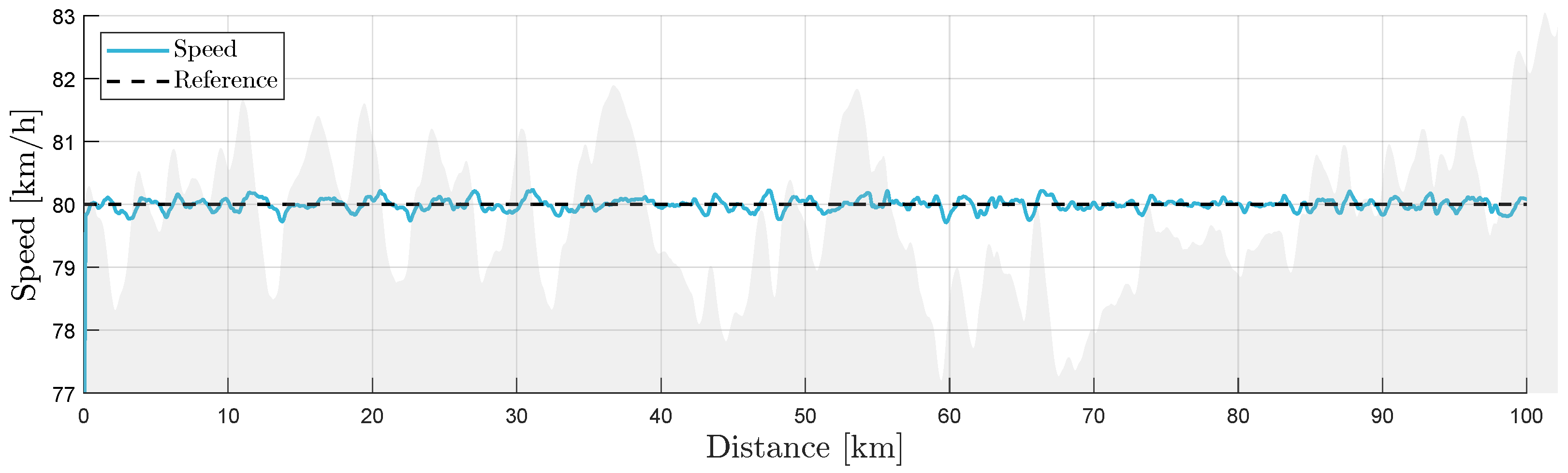
The vehicle speed was controlled by a PI regulator set to a reference of 80 km/h. The velocity tracking simulation result of a 40-ton battery electric truck is shown in Figure 24, with the altitude profile as a gray backdrop. The velocity profile was identical for each TMS considered.

To maintain the velocity reference when driving resistance forces act on the vehicle, the electric machine must either motor or act as a brake, where energy is recuperated. The electric machine power signal is shown in Figure 25. Positive and negative values for the electric machine power represent motoring mode and recuperation mode. The average power consumption of the vehicle was approximately 150 kW, a common figure for class 8 trucks in highway driving.

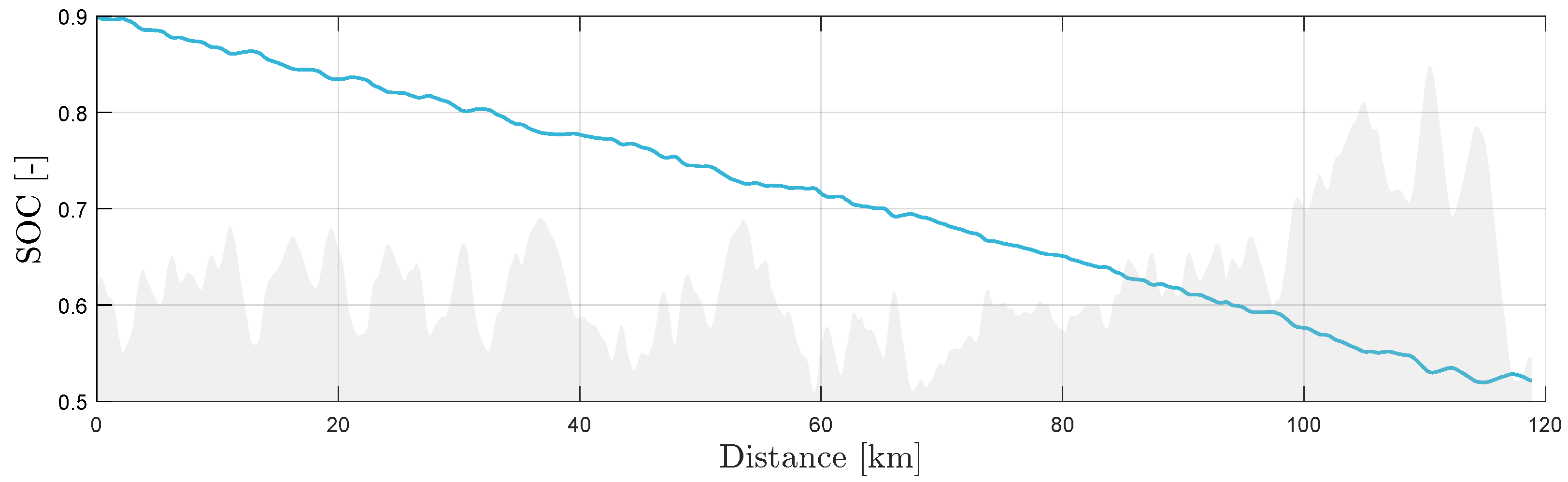
As the average power consumption was positive, the onboard energy storage was depleted during the mission. The state of charge is a common measure of available battery capacity and is shown in Figure 26. The mission started at 90% capacity. After 120 km, the state of charge reached fifty percent, suggesting a range of approximately 250 km.

The cabin compartment and battery back needed heating to maintain their temperatures. Heat was lost through convection from the battery and cabin to the ambient, in addition to the heat lost by maintaining a net flow of 300 m³/h flow of air through the cabin. The TMS was tasked to maintain temperature reference levels, in this case 23 °C for the cabin and 20 °C for the battery. The results for the pure electric heating case at $T_{\mathit{amb}}=-1$ °C is shown in Figure 27.

To maintain the battery and cabin temperatures, the performance of the three TMS architectures considered varied with ambient temperature and vehicle weight. Figure 28 shows the total energy efficiency (expended energy in kWh per 100 km driven), for vehicle weights of 20 tons (left) and 40 tons (right). The three thermal management architectures are separated by color. Each data point in the figure was collected by running a simulation for the specified technology, vehicle mass, and ambient temperature. Fifteen ambient temperatures were considered.

The main difference between the pure electric and heat pump cases was the expended compressor work. The total expended energy by the compressor is shown in Figure 29. The compressor work for the pure electric heating configuration was zero since no heat pump was used.

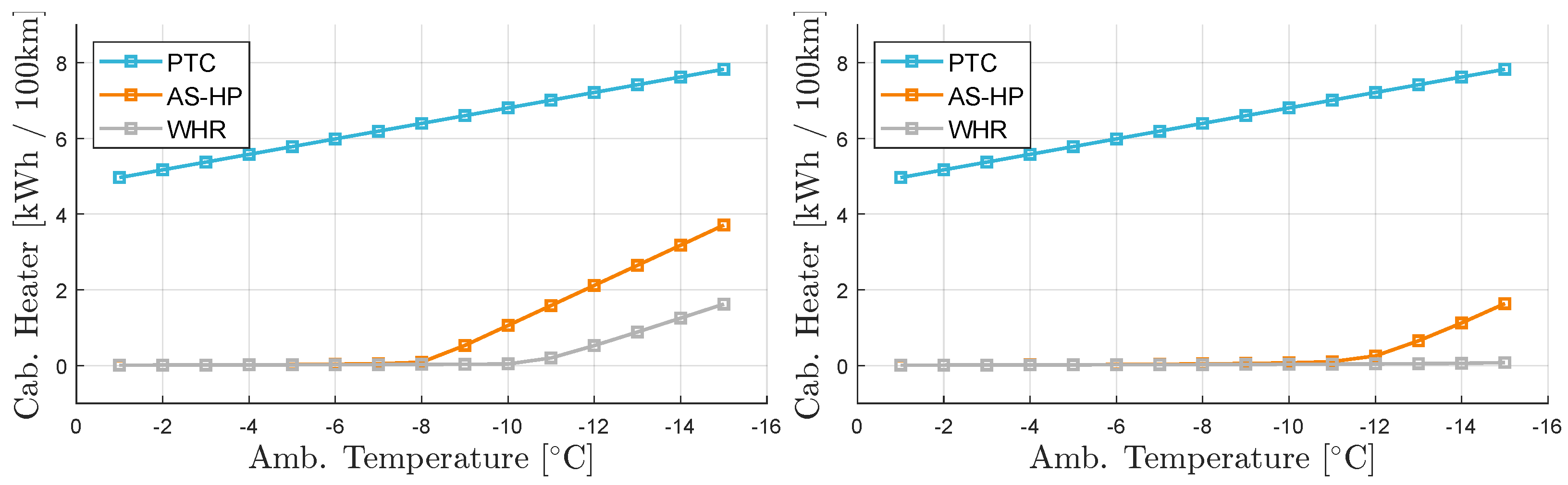
The performance gains or losses appeared as trade-offs between the compressors and heaters in the TMS. Figure 30 shows the total expended heating energy for the cabin heaters.

The heat pump coefficient of performance varies with ambient temperature. The coefficient of performance was calculated as the total heating energy from the cabin condenser over the total expended compressor work. The results are shown in Figure 31.

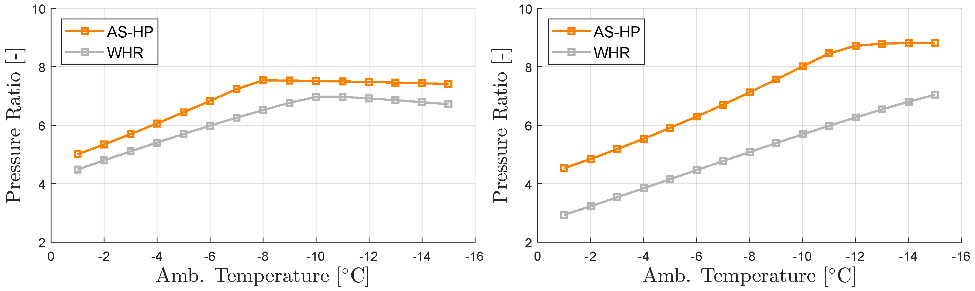
The refrigerant compressor work increases strongly with increasing compression pressure ratio. The pressure ratio over the compressor is shown in Figure 32. The pressure ratio was calculated as an average over the total driving mission.

The results show that for lighter and heavier battery electric trucks, the heat pump systems outperformed pure electric heating, and the waste-heat recovery system outperformed the air-sourced system. The benefit of using waste heat increased as ambient temperatures became colder. The performance of the waste-heat recovery and air-source systems were almost indistinguishable for 20-ton vehicles at −1 and −2 °C ambient temperatures.

The improvement in performance can be explained by the ratio of the compressor and electric heater work. The compressor work was higher for the lighter vehicle for both waste-heat recovery and the air-source heat pump, since the heavier vehicle produced more waste heat, requiring less external heating for the battery pack. For higher temperatures, the waste heat system required less compressor work than the air-source system, and vice versa for lower temperatures. For the lighter and heavier vehicles these crossover points occurred at $T_{\mathit{amb}}=-9$ °C and $T_{\mathit{amb}}=-14$ °C.

The crossover points for the compressor work matched the points at which additional electrical heating was required to maintain the temperature setpoints for the cabin and battery. For both lighter and heavier vehicles, the air-source heat pump system needed additional heating at higher ambient temperatures. The heavy vehicle equipped with waste-heat recovery did not need any electrical cabin heating for temperatures down to −15 °C.

The heat pump performance worsened for both heat pump systems as temperature decreased, as shown by the coefficient of performance in Figure 31, but the waste-heat recovery system outperformed the air-source heat pump system in terms of coefficient of performance.

4.4. Case Study 2: Cooling for Fuel Cell Hybrid Trucks

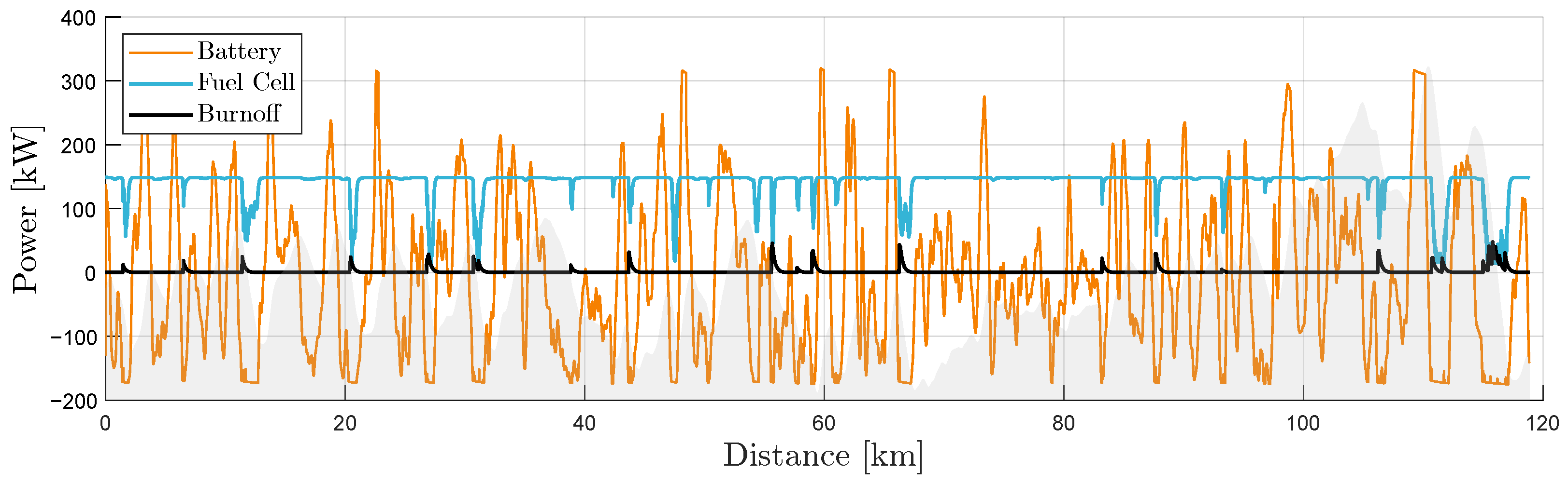
The fuel cell hybrid truck carried two onboard energy storage systems and needed a strategy for their respective control to match the total power demand, positive or negative. The result of this control strategy, for a 40-ton fuel cell truck at $T_{\mathit{amb}}=31$ °C, for the entire driving mission, is shown in Figure 33.

The fuel cell output a nominal power, while reducing its output when the battery was recuperating at maximum capacity. The nominal fuel cell power output level was tuned so that the state of charge was maintained at around half capacity. The state of charge of the battery corresponding to Figure 33 is shown in Figure 34.

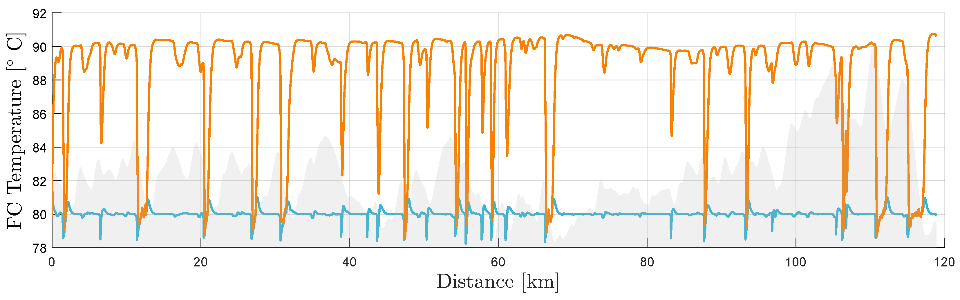
Heat is produced when energy is converted in the fuel cell, battery, and motor. The TMS’s task is to transfer this heat to the ambient environment through the radiators. As the ambient temperature increases, the potential cooling power decreases. The fuel cell temperature is shown in Figure 35, where the temperature reference is 80 °C. The figure shows the temperature traces of a case where $T_{\mathit{amb}}=31$ °C (blue), and $T_{\mathit{amb}}=45$ °C (orange).

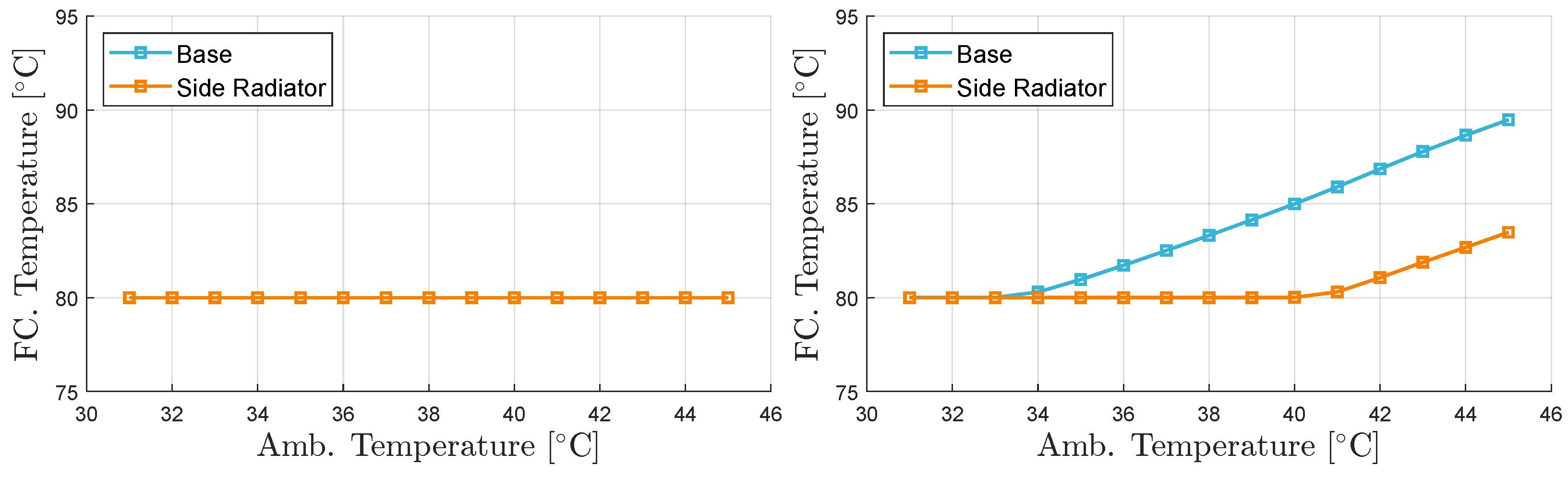
To evaluate the performance gains of including additional radiator area for the fuel cell hybrid truck, simulations were carried out for two vehicle weights and ambient temperatures varying from $T_{\mathrm{amb}}=31$ °C (blue) and $T_{\mathrm{amb}}=45$ °C. The average temperature for each simulation, calculated from the traces as shown in Figure 35, is shown in Figure 36.

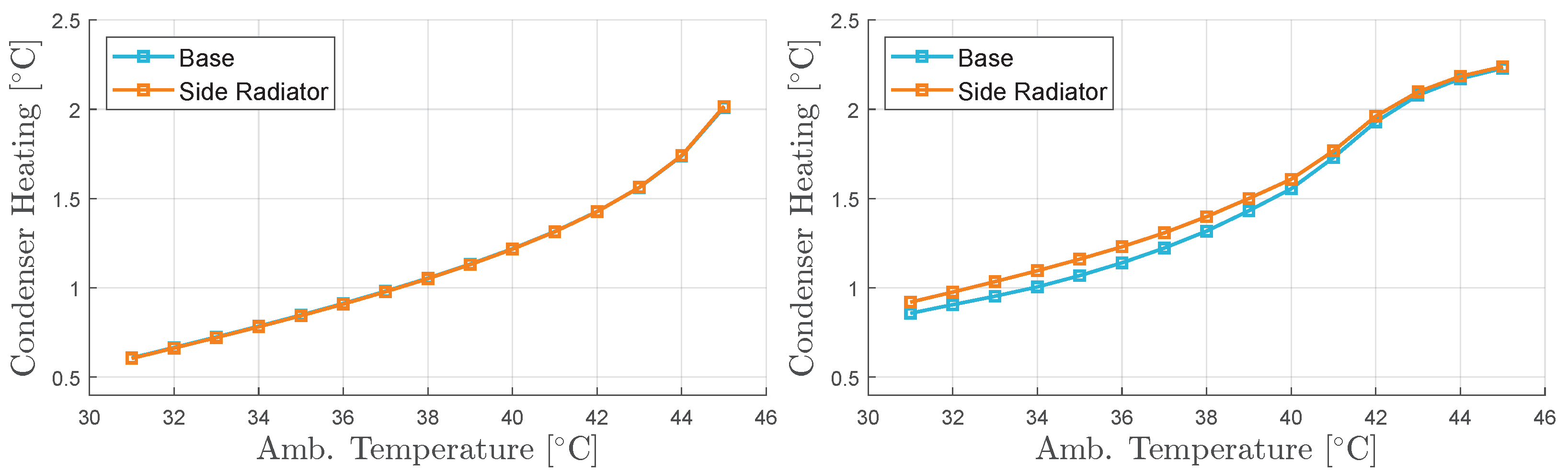
The front radiator is hidden by a condenser, used to cool the cabin and battery. The air temperature reaching the radiator is therefore slightly hotter than ambient temperature, depending on the refrigeration operating. The average condenser heating in degrees above ambient temperature is shown in Figure 37. The heating was calculated as an average over the mission.

The results show that the benefits of the additional radiator area were dependent on the vehicle weight. As shown in Figure 36, the lighter vehicle received no benefit from an extra radiator, while the heavier vehicle was able to maintain the fuel cell temperature up to $T_{\mathrm{amb}}=40$ °C.

5. Conclusions

As electric vehicle manufacturers continue to seek performance improvements, the onboard hardware and software systems become increasingly complex. The state of the art for electric vehicle TMSs has advanced considerably over the last twenty years. This complexity brings with it challenges in design, evaluation, and control. A model-based simulation method is one method to counter this challenge, by providing engineers an environment in which system designs and control algorithms can be evaluated quickly and simultaneously.

In this work, the state of the art of TMSs was investigated, both from an academic and industrial perspective. It was found that most systems relied on similar technologies to deal with the thermal management problem, namely, heat pumps and waste-heat recovery for battery electric heating, and additional radiators for fuel cell cooling.

With a clear picture of what features a state-of-the-art TMS should include, models were developed to suit those requirements, extending the ECCV platform with models that described coolant and refrigerant flow and heat transfer systems. In order to keep the simulation tool to native Matlab/Simulink, lookup maps for a common refrigerant were developed using multiparameter equations of state.

To demonstrate the simulation tool’s capability, the developed models were then used to build five TMSs for four vehicle configurations (light and heavy, battery electric and fuel cell hybrid), and the performance of the TMSs were evaluated. The results of the case studies showed that waste-heat recovery systems improved total energy efficiency, particularly in very cold environments, and that the benefits of using additional radiators for a fuel cell vehicle were conditional on the vehicle weight.