Abstract
Power system stability prediction leveraging deep learning has gained significant attention due to the extensive deployment of phasor measurement units. However, most existing methods focus on predicting either transient or voltage stability independently. In real-world scenarios, these two types of instability often co-occur, necessitating distinct and coordinated control strategies. This paper presents a novel concurrent prediction framework for transient and voltage stability using a spatio-temporal embedding graph neural network (STEGNN). The proposed framework utilizes a graph neural network to extract topological features of the power system from adjacency matrices and temporal data graphs. In contrast, a temporal convolutional network captures the system’s dynamic behavior over time. A weighted loss function is introduced during training to enhance the model’s ability to handle instability cases. Experimental validation on the IEEE 118-bus system demonstrates the superiority of the proposed method compared to single stability prediction approaches. The STEGNN model is further evaluated for its prediction efficiency and robustness to measurement noise. Moreover, results highlight the model’s strong transfer learning capability, successfully transferring knowledge from an N-1 contingency dataset to an N-2 contingency dataset.
1. Introduction
The continuous growth in global electricity demand drives power systems to operate under increasingly high-load conditions, often nearing their stability thresholds [1]. This trend imposes substantial pressure on the reliability and resilience of modern power grids, making it imperative to address the challenges associated with maintaining stable operations. The integration of renewable energy sources (RESs), such as wind and solar power, further complicates this landscape due to their inherent intermittency and variability. While these sources offer significant environmental advantages, they introduce dynamic behaviors that, if not carefully managed, can undermine grid stability. Moreover, the widespread adoption of power electronic devices exacerbates these challenges by introducing rapid and nonlinear dynamics that may interact detrimentally with the grid [2]. Consequently, ensuring the stability of power systems under such conditions has become a paramount concern for researchers and practitioners. Accurate prediction of power system stability has become increasingly vital, as it enables operators to implement timely and effective control measures, thereby ensuring reliable electricity delivery and mitigating the risk of cascading failures [3].
Traditional model-based stability prediction methods can be categorized into time-domain simulation and energy function approaches [4]. Time-domain methods typically use low-order models to simulate system stability. For instance, C.-W. Liu and J. S. Thorp employed an implicit decoupling PQ method for stability prediction while utilizing a linear model for parallel simulation approach [5] to predict stability in the IEEE 145-bus system [6]. Time-domain simulation methods require detailed system models to solve differential or algebraic equations. However, with the continuous expansion of modern power systems and the integration of RESs, obtaining detailed models becomes impractical, and the solution process is time-consuming [2]. Energy function methods are generally based on Lyapunov’s second law. The Lyapunov exponent’s out-of-step technique [7] is used to predict system stability and energy functions [8] are employed to estimate stability margins for predicting stability in the IEEE 39-bus system. In large-scale power systems, determining an appropriate Lyapunov function is challenging, and the computation of system energy is highly time-consuming [9]. However, traditional methods have significant limitations. They require precise power system models, and inaccuracies can lead to unreliable stability analysis. Additionally, their computational time increases with system size, making them unsuitable for real-time applications in modern, large-scale power systems.
With the deployment of phasor measurement units (PMUs) and the development of wide-area monitoring systems (WAMS), machine learning (ML) has been extensively applied to power system stability prediction. ML methods are data-driven and model-free, making them well-suited for online use, where fast response times and high accuracy are required. A.Karami employed a multi-layer perceptron (MLP) to estimate the transient stability margin of power systems [10]. Convolutional neural networks (CNNs) are utilized for transient stability prediction [11]. Machine learning techniques are applied to predict voltage stability in power systems [12], while G. Wang et al. leveraged graph convolutional networks (GCN) and long short-term memory (LSTM) networks for online voltage stability prediction [13]. ML methods do not rely on the detailed modeling of power systems and possess strong generalization capabilities, making them highly promising for online diagnostics [14]. Farheen Bano et al. analyzed microgrid voltage stability using a variety of machine learning models, including random forest, gradient boosting, K-means, hierarchical clustering, and regression models [15].
Short-term power system instability includes transient and voltage instability [16]. Transient instability occurs when, after a large disturbance, the generators in the power system fail to maintain synchronous operation, causing the system to become unstable. Voltage instability occurs when a disturbance leads to a significant voltage drop, potentially resulting in voltage collapse. When a fault occurs in the system, transient and voltage instability often manifest simultaneously, or the system may transition from one instability mode to another. Different instability types require distinct control strategies [16]. For transient stability, the objective is to maintain generator synchronization, and control strategies typically focus on the generator rotor, such as excitation control or early disconnection of critical generators [2]. For short-term voltage stability, the focus is on controlling reactive power, which can be achieved by deploying reactive power compensation devices, such as capacitors, reactors, or emergency load shedding [17]. However, achieving precise classification of power system stability remains a complex challenge [18]. For instance, when the rotor angles of two generators gradually separate, the electrical distance between them increases, causing voltage drops at intermediate load nodes. This issue, caused by transient power angle instability, cannot be effectively resolved by reactive power compensation alone at the critical load node [19]. Therefore, precise classification of power system stability behaviors is crucial for successful operation.
Although current deep learning-based methods for single instability prediction perform relatively well, they focus on individual stability, such as transient or voltage stability, often overlooking the interrelated nature of instability behaviors. The coupling between phase angle and voltage instabilities is well-established, and neglecting this aspect can lead to incomplete or inaccurate control strategies. Moreover, deep learning models face the challenge of imbalanced data, as instability events are rare in power system operations. This imbalance often results in overfitting, reducing model generalizability to unseen scenarios. Current methods have not sufficiently addressed this issue, which limits their robustness in real-world applications. Furthermore, the practical applicability of these methods under more complex conditions, such as N-2 contingencies, remains underexplored. Given the significant impact of such contingencies on system stability, further research is necessary to improve the reliability and scalability of deep learning-based approaches in handling these complex scenarios. This paper proposes a co-prediction of transient and voltage stability based on a spatio-temporal embedding graph neural network (STEGNN). The main contributions of this paper are as follows:
(1) The STEGNN model proposed combines power system topology with PMU historical data to co-predicate transient and voltage stability, enabling a comprehensive analysis of power system dynamic stability for more precise operational decisions in the event of system instability.
(2) In power system operation data, instability samples constitute a small proportion. During the training process, a weighted loss function is adopted to emphasize unstable samples, effectively addressing the data imbalance issue, which enhances the model’s training stability and prevents overfitting.
(3) The proposed STEGNN model is designed for real-time applications, ensuring that it balances prediction accuracy and computational efficiency. By selecting an optimal observation window length, the model provides timely and accurate transient and voltage stability predictions, making it suitable for real-time monitoring and control in power systems.
(4) The STEGNN model is pre-trained on the N-1 contingency dataset and successfully applied to the N-2 contingency dataset, validating its effectiveness in handling various contingency scenarios and demonstrating its strong transferability.
2. Spatiotemporal Embedding Graph Neural Network
We propose a STEGNN framework for co-predicting the transient and voltage stability assessment. The structure of the STEGNN framework is presented below. STEGNN mainly consists of three parts: the multi-head GCN modules as topological features extractors, the temporal convolution networks (TCN) module as a temporal features extractor, and the MLP layer as the classifier. The co-prediction framework and the STEGNN model are shown in Figure 1. The structure has three main parts: the GC module, TC module, and MLP prediction layer. Each GC module has five neurons, where and (i = a to e) represent the input states of the five neurons in each GC module. The operation of the GC module is to update the output state of the focused neurons (red) using the adjacency matrix, which is only relevant to the adjacent neurons (blue) rather than others (gray). The topological features are then extracted by the FC layer and processed by the TC module, which is composed of R residual blocks with dilated factors to . In the end, the MLP layer generates the prediction probability function.
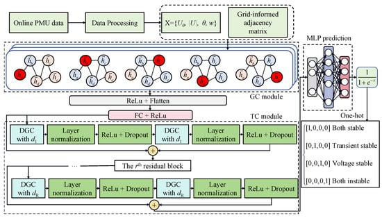
Figure 1.
The power system stability co-prediction process and details of the STEGNN model.
2.1. Preliminary DL Techniques
The framework of the proposed STEGNN model consists of GC and TC modules based on GCN [20] and TCN [21]. The fundamental concepts of GCN and TCN provide a foundation for understanding the STEGNN model. MLP is the classifier for the transient stability prediction.
GCN structure: The structure of the GCN layer can be represented as an undirected graph , where is the set of neurons, is the set of neuron connections, and is the adjacency matrix [22]. To represent the neuron connections in a GCN layer, the re-normalized adjacency matrix is often used:
where is the adjacency matrix with self-loops, and is the identity matrix. is the diagonal degree matrix, where . The core idea of a GCN is to map a input matrix to a new output feature matrix for the nodes in the graph, where R and S represent the input and output feature dimensions, respectively. The layer function of GCN is defined as follows:
where , , , and represent the input, output, network weights, and bias, respectively. is the ReLU activation function.
TCN structure: The TCN model consists of sequential residual blocks, each containing a 1D fully convolutional network (FCN) [23] that uses causal and dilated convolutions and a residual connection. The causal convolution ensures that the output has the same length as the input and considers the entire history while preserving the causality of the sequence. Dilated convolutions are employed to address the depth burden introduced by causal convolutions. Dilated convolutions expand the receptive field exponentially, allowing the model to consider a larger portion of the history with a smaller depth. Specifically, the dilated convolution operation applied to the j-th element in the 1D sequence , using a filter , is defined as follows:
where k is the filter size and d is the dilation factor. The dilation factor expands the receptive field, allowing the model to capture a broader input range than standard convolutions. Residual connections stabilize deep causal dilated convolutions, enabling the layers to learn adjustments to the identity mapping. Additionally, a convolution layer, denoted as , is introduced to resolve any dimensional mismatches between the input and output. Consequently, the output of a residual block is defined as follows:
where and are the input and output of the residual block, and refers to layer normalization.
MLP structure: An MLP consists of an input layer, one or more hidden layers, and an output layer.
Input layer: The input layer accepts the input vector .
Hidden layers: Each hidden layer performs a linear transformation followed by a nonlinear activation function. The output of the l-th hidden layer is defined as follows:
where is the weight matrix, is the bias vector, and represents the activation function (e.g., ReLU, sigmoid, and tanh).
Output layer: The output layer generates the final output vector :
where L is the total number of layers.
2.2. STEGNN Framework
The proposed STEGNN model extracts the topological spatial features from the multivariate physical PMU data input using GC modules, composed of two GCN layers and one fully connected (FC) layer with relu activations [24].
Then, the TC module follows the GC modules, located after the convenience of l topological features extracted by GC modules, which were introduced in the former part. The last one is the MLP module after the TC module. MLP modules are adopted to integrate the topological and temporal features extracted by both the GC and TC modules. Finally, the softmax activation generates the prediction as a probability function.
Class-weighted loss function: Since STEGNN’s transient stability prediction gives a multi-stability probability, the class-weighted category cross-entropy (CCE) is the loss function with the regularization. Then, the loss function is defined as follows:
where and denote the label and the model output of the jth category sample, and represents category weight factors, . Additionally, and serve as learnable network parameters, where is the regularization weight.
Grid-informed adjacency matrix: In spatial feature extraction within the GC modules, three distinct grid-informed adjacency matrices, , have been conceptualized, considering a power system’s electrical and structural attributes. Initially, drawing from reference, a binary adjacency matrix with self-connections for a power system is selected (referred to as ). The elements of this matrix are defined by Equation (9), which accounts for the system’s topological structure while disregarding the edge weights. Subsequently, the concept of is introduced, where the active power flows are integrated as weights into the adjacency matrix, as articulated in Equation (10). Lastly, the adjacency matrix is formulated by incorporating the maximum transmission capacity of transmission lines as off-diagonal elements, complemented by the active power injections for the diagonal elements, as delineated by Equation (11). This approach comprehensively represents the power system’s spatial characteristics for enhanced feature extraction.
where denotes the ensemble of transmission lines operating under normal conditions. In contrast, represents the set of transmission lines that are compromised during contingencies. The notation signifies the transmission line interconnecting nodes i and j within the network. The variable corresponds to the maximum permissible transmission capacity for the line connecting these two nodes. Additionally, and represent the active power injections at nodes i and j, respectively. If a transmission line is an element of the set , it is characterized as being in a state of malfunction during the contingency scenario. This classification is crucial for analyzing power system resilience and developing strategies to mitigate the impact of such disruptions.
2.3. Data Representation and Label Definition
The inputs to the proposed co-prediction framework are the feature matrix of transient dynamics time series data:
where , F is the number of features, and N is the number of nodes. The jth column of is the post-fault time series with length l describing one of the PMU data streams of node j, in power systems. Thus, we choose the bus relative phase, bus voltage magnitude, rotor angles, and rotor speed as the second input , where .
The transient stability of power systems is decided by the transient stability index (TSI) as [11]
where is the maximum absolute value of the difference between the rotor angles of any two synchronous motors during the simulation process. The is also indicated by the sign of ,
The voltage stability of power system depends on the voltage magnitude dip at any bus within the evaluation period [25].
where is typically defined as 50 cycles or 1000 ms, with 1000 ms adopted in this study.
As shown in Table 1, the label y for supervising the model training is a one-hot variable, i.e., four classes are considered according to the stability condition of transient stability label and voltage stability label . The prediction of the STEGNN model, , is the probability that the power system will evolve to one of the four stability conditions after the softmax calculation of the last layer output of the proposed network:

Table 1.
Definition of label y as the one-hot form.
The power system stability co-prediction process and the detailed STEGNN model are depicted in Figure 1. The proposed framework utilizes online PMU data to derive the feature matrix , as defined in Equation (12), and labels the stability states according to Table 1. The adjacency matrix is constructed based on the power system topology, as defined in Equations (9)–(11). The inputs and are fed into the STEGNN model, where a weighted loss function is used for training, as described in Equation (8). During testing, one-hot encoding is applied to represent the predicted stability states of the power system.
3. Case Studies
The experimental results of the IEEE 118-bus power system are used to evaluate the proposed STEGNN model. We evaluate the model’s performance on the stability co-prediction and benchmark it with a single stability prediction. Additionally, we discuss the impact of grid-informed adjacency matrices and the time length of input PMU data on the STEGNN model’s performance. We also discuss the model’s robustness to noise. N-1 contingencies are considered, and the transient fault dynamics of the power system are simulated in the PSS/E program as follows:
- (1)
- The consumed power randomly varies between 80% and 120% of the base load levels, repeated for 50 iterations;
- (2)
- The load flow equation is solved to adjust the generator outputs accordingly;
- (3)
- Three phase-to-ground faults are applied at all 118 buses and the ends of 177 transmission lines, with random fault clearance times of 0.3, 0.4, 0.5, or 0.6 s;
- (4)
- The simulation is run for 5 s, and both transient stability and voltage stability labels are set.
Consequently, 59,000 samples are generated, and the number of four classes is 35381, 6389, 701 and 16,529, where the proportions of the training set, validation set, and test set are 80%, 10%, and 10%, respectively.
The confusion matrix is a valuable tool for evaluating the prediction model, defining four key values based on actual and predicted outcomes: true positive (), false positive (), true negative (), and false negative (). Here, or represents the instances where the model correctly predicts the positive or negative class. At the same time, or corresponds to instances where the model incorrectly predicts the negative or positive class. Stable (positive) and unstable (negative) are used interchangeably. To assess the performance of the STEGNN model, four metrics are employed: accuracy (), false positive rate (), false negative rate (), and F-score () where
where denotes the fraction of among the models classified as positive class, and denotes the fraction of among the total number of positive samples. While , , and can reveal whether the predictions are good or not, could evaluate the prediction of the model of imbalanced samples more comprehensively, for it indicates how much more important recall is than precision or vice versa. We set in this paper. The STEGNN model is trained on the NVIDIA GeForce RTX 4090 platform with the Tensorflow 2.3.1 environment and the model training hyperparameters are shown in Table 2.

Table 2.
The detailed seven main hyperparameters and construction of STEGNN.
3.1. Concurrent Prediction Performance
ACC and loss curves during the training and validation process are shown in Figure 2a. ACC and loss denote the validation dataset’s prediction accuracy rate and class-weighted CCE. The confusion matrix for the co-prediction is given in Figure 2b.
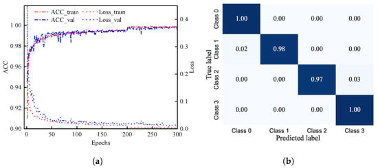
Figure 2.
Training results of the STEGNN model. Subfigure (a) shows accuracy and loss for the stability co-prediction on both the training set and validation set. Subfigure (b) shows the confusion matrix of the test set, where Class 0, Class 1, Class 2, and Class 3 represent [1, 0, 0, 0], [0, 1, 0, 0], [0, 0, 1, 0], and [0, 0, 0, 1] in Table 1. (a) ; (b) confusion matrix.
To evaluate the effectiveness of the STEGNN model, a performance comparison is conducted between the proposed method and four existing deep learning models: MLP, CNN, TCN, and GCN. Concurrent transient stability prediction (Co-TSP) and voltage stability prediction (Co-VSP) are performed on the IEEE-118 bus power system using identical training, evaluation, and test datasets, as well as the same experimental setup. The results are presented in Table 3. As shown in Table 3, the STEGNN model outperforms the other methods in both transient stability and voltage stability prediction and the results of prediction are shown in bold.

Table 3.
Comparison of STEGNN with other deep learning methods.
In the IEEE 118-bus power system, the dataset of transmission line ground faults at 0.2 s (TLGF-0.2) has a size of 1770 and simultaneously has transient and voltage stability status labels. Compared to the concurrent prediction model trained with the dataset of the joint labels of transient stability and voltage stability, the single TSP and VSP prediction models are trained with the datasets with the single stability labels for the transient stability and voltage stability, respectively. In Table 4, it can be observed that the concurrent STEGNN prediction model, co-prediction, can predict the TSP and VSP simultaneously for the TLGF-0.2 dataset, while the combined prediction of the single TSP and single VSP respectively recorded 23 and 38 incorrect predictions and 54 errors in total for TSP and VSP. In Table 5 and Table 6, the co-TSP and co-VSP predictions perform better than the single TSP and single VSP. As for the joint prediction, the concurrent STEGNN model can make the perfect prediction for the TLGF-0.2 test dataset. The concurrent prediction method demonstrates superior performance in transient stability, voltage stability, and co-prediction. The results of the joint prediction in Table 4, Table 5 and Table 6 are all optimal, and are presented in bold.

Table 4.
The performance comparison of the combined result of the single TSP and the VSP with the concurrent TSP and VSP for the IEEE 118-bus power system based on the TLGF-0.2 dataset.

Table 5.
The performance comparison of the single TSP and co-TSP for the IEEE 118-bus power system based on the TLGF-0.2 dataset.

Table 6.
The performance comparison of the single VSP and co-VSP for the IEEE 118-bus power system based on the TLGF-0.2 dataset.
Figure 3 provides a visualization of the high-dimensional features extracted from the hidden layers of the STEGNN model. The training and testing datasets samples are color-coded according to their true labels and predictions, visually assessing the model’s learning process. In the two subplots in the first row of Figure 3, the training and testing samples are colored based on their true labels, while the second row shows the same datasets colored according to the predicted output with the STEGNN model. The two subplots in the third row of Figure 3 show the prediction error. The results in Figure 3 demonstrate that the STEGNN model successfully learns the underlying features of the dataset and makes accurate predictions.
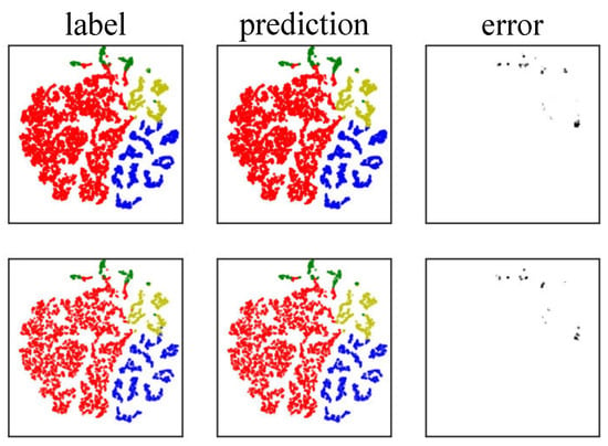
Figure 3.
Visualization of high-dimension features from the hidden layer. The first row is training and testing dataset samples colored with labels, and the second row is training and testing dataset samples colored with network outputs.
3.1.1. Effect of Time Length
The observation window length of post-fault PMU data directly impacts the real-time application of the proposed STEGNN model. A longer observation window provides more system dynamics information, which enhances prediction (), as shown in Table 7. However, it also increases computational training time, as illustrated in Figure 4. While the training time itself does not affect real-time applications, it may become significant when scaling to larger power systems, increasing the overall computational cost.

Table 7.
The concurrent prediction performance with different time lengths of post-fault PMU data in the IEEE 118-bus power system.
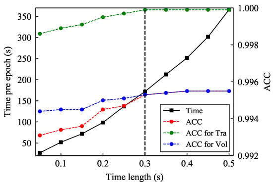
Figure 4.
ACC and computational training time per epoch with different time lengths for the proposed STEGNN model trained in the IEEE 118-bus power system.
As depicted in Figure 4, when the time length is less than 0.3 s, the shows a steady increase. Beyond 0.3 s, the plateaus, providing diminishing returns despite the additional observation data. To balance the demands of real-time application and predictive performance, a time length of 0.3 s is chosen and the prediction effect for time length of 0.3s is shown in bold. This selection ensures high prediction accuracy while limiting the computational cost associated with larger power systems, thereby maintaining the practical feasibility of the model.
3.1.2. Sensitivity Analysis
For the co-prediction of transient stability and voltage stability in practical power systems, the presence of noise in PMU data significantly impacts the prediction model performance. The standard deviation of noise in PMU data typically ranges from 0.0005 to 0.01, corresponding to a signal-to-noise ratio (SNR) of approximately 45 dB [26]. Table 8 presents the co-prediction performance of the IEEE 118-bus power system under various SNR levels. Even at an SNR of 50 dB (slightly lower than typical levels), the model maintains high accuracy, with the ACCs of transient stability prediction (TSP) and voltage stability prediction (VSP) decreasing by only 0.01% and 0.03%, respectively. Under high-noise conditions at an SNR of 20 dB, the prediction performance exhibits a moderate decline, with ACCs decreasing by 0.14% and 1.22%. Additionally, other evaluation metrics also show degradation as the SNR decreases for co-TSP and co-VSP. These results demonstrate that STEGNN exhibits strong robustness against noise.

Table 8.
Performance on co-prediction in the IEEE 118-bus power system under different SNR levels of PMU data.
3.2. Performance in N-2 Contingency
The N-2 dataset, obtained from simulating three-phase grounding at two random buses in the IEEE 118-bus system, contains 29,500 samples. We evaluated and compared the ACC of co-prediction, single prediction, and co-prediction without a weighted loss function based on the STEGNN model. Figure 5 shows that co-prediction performs best transferability for the N-2 dataset. All methods achieve high VSP accuracy, with the main differences observed in TSP. The ACC of co-prediction surpasses that of single prediction by 22.4%. It indicates a coupling relationship between transient and voltage stability and co-prediction significantly improves model transferability. Additionally, the ACC of co-prediction exceeds that of co-prediction without weighted loss by 32.3%, highlighting the importance of a weighted loss function for imbalanced datasets.
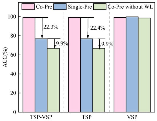
Figure 5.
The ACC of different methods for the N-2 contingency dataset. Co-Pre, Single-Pre, and Co-Pre without WL are abbreviations for co-prediction, TSP/VSP single prediction, and co-prediction without weight loss, respectively. TSP-VSP Co-Pre represents the co-prediction for transient and voltage stability, and the TSP–VSP single prediction represents the combined result of the single TSP and the single VSP. TSP Co-Pre represents Co-TSP, and VSP Co-Pre represents Co-VSP. TSP Single-Pre represents the single TSP and VSP Single-Pre represents the single VSP.
3.3. Effect of Grid-Informed Adjacency Matrices
In Figure 6, three grid-informed adjacency matrices are introduced, incorporating the power grid’s structural and electrical parameter information. The grid-informed adjacency matrices are introduced in Figure 6, where the colors of each small pixel block represent the corresponding element value of the four adjacency matrices. The corresponding prediction performances are shown in Table 9. It can be observed from Table 9 that the adjacency matrix shows the worst performance. This can be explained by the very sparse adjacency matrix visualization in Figure 6, which indicates that although contains information on active power flow distribution, other useful information about the power system topology and electrical properties is discarded. Under the same training conditions, demonstrates superior performance compared to . Therefore, the STEGNN model uses as the power grid information adjacency matrix for the co-prediction of the power system stability.
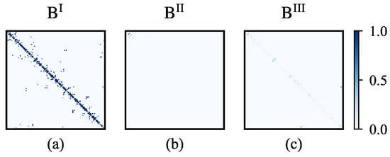
Figure 6.
Visualization of grid-informed adjacency matrices, where subfigure (a) shows , subfigure (b) shows , and subfigure (c) shows .

Table 9.
Performance comparison of grid-informed adjacency matrices.
Table 9 presents a comparison of the joint prediction performance of the concurrent STEGNN model as well as the performance of co-TSP and co-VSP using three different grid-informed adjacency matrices for the IEEE-118 bus power system and the predictions of grid-informed adjacency matrice using are shown in bold. The performance is evaluated using three metrics: , , and . The joint prediction of TSP and VSP is 99.28%. The co-TSP and co-VSP perform very well. The of the co-TSP and co-VSP are 99.97% and 99.31%, respectively.
3.4. Effect of Weighted Loss
Figure 7 illustrates the impact of weighted loss on the STEGNN model during training. Figure 7a shows the ACC of co-prediction, co-TSP, and co-VSP. It can be observed that the ACC remains high whether weighted loss is applied, which, to some extent, demonstrates the superiority of the STEGNN model. The ACC is higher when the weighted loss is used. Figure 7b shows the FPR for co-TSP and co-VSP. The results indicate that without weighted loss, the FPR is significantly higher. This suggests when transient or voltage instability occurs, models without weighted loss fail to provide adequate warnings, which is hazardous and unacceptable.
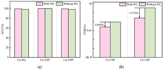
Figure 7.
Subfigure (a) shows the of STEGNN with and without weighted loss. Subfigure (b) shows of STEGNN with and without weighted loss, and WL is short for weighted loss. (a) comparison; (b) comparison.
4. Conclusions
In conclusion, the proposed spatiotemporal enhanced graph neural network (STEGNN) model effectively addresses the intricate challenges of concurrent transient and voltage stability prediction in power systems. The model enables comprehensive and accurate stability assessments by seamlessly integrating spatial features derived from power system topology with temporal dynamics captured from PMU data. This dual-perspective approach enhances predictive precision while capitalizing on the interdependencies between transient and voltage stability, resulting in robust and dependable performance.
The STEGNN framework employs a cohesive integration of spatial and temporal information. Spatial features are extracted via a graph convolution (GC) module, while temporal data from PMUs are processed through a temporal convolution (TC) module. This synergistic design allows for a unified and accurate analysis of both stability phenomena. The model’s capability to simultaneously predict transient and voltage stability delivers several distinct advantages:
1. Superior predictive accuracy: The STEGNN framework outperforms traditional single-focus stability prediction methods for transient stability prediction (TSP) and voltage stability prediction (VSP). By jointly analyzing transient and voltage stability, the model harnesses inherent correlations, such as those between rotor angle dynamics and voltage behavior, to produce more precise and reliable predictions.
2. Real-time prediction capability: The STEGNN model facilitates rapid stability assessments using solely PMU data, making it highly suitable for real-time and online applications. This swift response capability is critical for system operators, enabling proactive interventions and preventive measures to mitigate potential instabilities and enhance grid reliability.
3. Robustness and transferability: To address the issue of limited, unstable samples, a weighted loss function is employed to enhance the model’s generalization ability. The model exhibits exceptional resilience to noise in PMU measurements, a critical attribute for real-world implementation in operational power systems where data imperfections are unavoidable. This robustness ensures consistent performance under varying conditions. Furthermore, the STEGNN framework demonstrates strong adaptability, maintaining high accuracy when applied to more complex and dynamic system scenarios.
The STEGNN’s ability to deliver timely and reliable stability predictions establishes it as a vital tool for system operators managing increasingly complex and interconnected power grids. Its robustness to data noise and unified treatment of transient and voltage stability enhance its practical utility, ensuring reliable operation even in challenging environments. By addressing these critical aspects of power system stability, the STEGNN framework contributes significantly to the operational resilience and security of modern and future energy systems, aligning with the evolving demands of smarter, more interconnected grids.
Author Contributions
Conceptualization: C.D., L.D., W.C., J.H. and X.C.; Methodology: C.D., L.D., W.C. and X.C. Resources: J.H., J.W. and L.L.; Formal Analysis: J.W. and W.Q; Validation: L.L., W.Q. and S.L.; Data Analysis: W.Q. and S.L.; Original Draft Preparation: X.C., S.L. and W.Q.; Writing—Review and Editing: X.C., C.D., W.Q. and S.L. All authors have read and agreed to the published version of the manuscript.
Funding
This research was supported by the Science and Technology Project of State Grid Fujian Power Co., Ltd. of China (521304240018), which is named Research on an Artificial Intelligence Joint Prediction Method for Transient Stability Based on Physics Driven Feature Engineering.
Data Availability Statement
The original contributions presented in this study are included in the article. Further inquiries can be directed to the corresponding author.
Conflicts of Interest
Author Lanxin Lin was employed by the company State Grid Fujian Electric Power Co., Ltd. Fuzhou Company. The remaining authors declare that the research was conducted in the absence of any commercial or financial relationships that could be construed as a potential conflict of interest.
References
- Das, S.; Ketan Panigrahi, B. Prediction and control of transient stability using system integrity protection schemes. IET Gener. Transm. Distrib. 2019, 13, 1247–1254. [Google Scholar] [CrossRef]
- Zhu, L.; Hill, D.J.; Lu, C. Hierarchical deep learning machine for power system online transient stability prediction. IEEE Trans. Power Syst. 2019, 35, 2399–2411. [Google Scholar] [CrossRef]
- Hooshyar, H.; Savaghebi, M.; Vahedi, A. Synchronous generator: Past, present and future. In AFRICON 2007; IEEE: Piscataway, NJ, USA, 2007; pp. 1–7. [Google Scholar]
- Sobbouhi, A.R.; Vahedi, A. Transient stability prediction of power system; A review on methods, classification and considerations. Electr. Power Syst. Res. 2021, 190, 106853. [Google Scholar] [CrossRef]
- Zadkhast, P.; Jatskevich, J.; Vaahedi, E. A multi-decomposition approach for accelerated time-domain simulation of transient stability problems. IEEE Trans. Power Syst. 2014, 30, 2301–2311. [Google Scholar] [CrossRef]
- Liu, C.-W.; Thorp, J.S. New methods for computing power system dynamic response for real-time transient stability prediction. IEEE Trans. Circuits Syst. Fundam. Theory Appl. 2000, 47, 324–337. [Google Scholar]
- Yan, J.; Liu, C.-C.; Vaidya, U. Pmu-based monitoring of rotor angle dynamics. IEEE Trans. Power Syst. 2011, 26, 2125–2133. [Google Scholar] [CrossRef]
- Bhui, P.; Senroy, N. Real-time prediction and control of transient stability using transient energy function. IEEE Trans. Power Syst. 2016, 32, 923–934. [Google Scholar] [CrossRef]
- Farantatos, E.; Huang, R.; Cokkinides, G.J.; Meliopoulos, A. A predictive generator out-of-step protection and transient stability monitoring scheme enabled by a distributed dynamic state estimator. IEEE Trans. Power Deliv. 2015, 31, 1826–1835. [Google Scholar] [CrossRef]
- Karami, A. Tability margin estimation using neural networks. Int. J. Electr. Power Energy Syst. 2011, 33, 983–991. [Google Scholar] [CrossRef]
- Gupta, A.; Gurrala, G.; Sastry, P. An online power system stability monitoring system using convolutional neural networks. IEEE Trans. Power Syst. 2018, 34, 864–872. [Google Scholar] [CrossRef]
- Malbasa, V.; Zheng, C.; Chen, P.-C.; Popovic, T.; Kezunovic, M. Voltage stability prediction using active machine learning. IEEE Trans. Smart Grid 2017, 8, 3117–3124. [Google Scholar] [CrossRef]
- Wang, G.; Zhang, Z.; Bian, Z.; Xu, Z. A short-term voltage stability online prediction method based on graph convolutional networks and long short-term memory networks. Int. J. Electr. Power Energy Syst. 2021, 127, 106647. [Google Scholar] [CrossRef]
- Sarajcev, P.; Kunac, A.; Petrovic, G.; Despalatovic, M. Power system transient stability assessment using stacked autoencoder and voting ensemble. Energies 2021, 14, 3148. [Google Scholar] [CrossRef]
- Bano, F.; Rizwan, A.; Serbaya, S.H.; Hasan, F.; Karavas, C.-S.; Fotis, G. Integrating microgrids into engineering education: Modeling and analysis for voltage stability in modern power systems. Energies 2024, 17, 4865. [Google Scholar] [CrossRef]
- Kundur, P.; Paserba, J.; Ajjarapu, V.; Andersson, G.; Bose, A.; Canizares, C.; Hatziargyriou, N.; Hill, D.; Stankovic, A.; Taylor, C. Definition and classification of power system stability IEEE/CIGRE joint task force on stability terms and definitions. IEEE Trans. Power Syst. 2004, 19, 1387–1401. [Google Scholar]
- ALShamli, Y.; Hosseinzadeh, N.; Yousef, H.; Al-Hinai, A. A review of concepts in power system stability. In Proceedings of the 2015 IEEE 8th GCC Conference & Exhibition, Muscat, Oman, 1–4 February 2015; IEEE: Piscataway, NJ, USA, 2015; pp. 1–6. [Google Scholar]
- Abdi-Khorsand, M.; Vittal, V. Identification of critical protection functions for transient stability studies. IEEE Trans. Power Syst. 2017, 33, 2940–2948. [Google Scholar] [CrossRef]
- Atputharajah, A.; Saha, T.K. Power system blackouts-literature review. In Proceedings of the 2009 International Conference on Industrial and Information Systems (ICIIS), Peradeniya, Sri Lanka, 28–31 December 2009; IEEE: Piscataway, NJ, USA, 2009; pp. 460–465. [Google Scholar]
- Wu, Z.; Pan, S.; Chen, F.; Long, G.; Zhang, C.; Philip, S.Y. A comprehensive survey on graph neural networks. IEEE Trans. Neural Networks Learn. Syst. 2020, 32, 4–24. [Google Scholar] [CrossRef] [PubMed]
- Tang, X.; Chen, H.; Xiang, W.; Yang, J.; Zou, M. Short-term load forecasting using channel and temporal attention based temporal convolutional network. Electr. Power Syst. Res. 2022, 205, 107761. [Google Scholar] [CrossRef]
- Kipf, T.N.; Welling, M. Semi-supervised classification with graph convolutional networks. In Proceedings of the 5th International Conference on Learning Representations, ICLR, Toulon, France, 24–26 April 2017. [Google Scholar]
- Long, J.; Shelhamer, E.; Darrell, T. Fully convolutional networks for semantic segmentation. In Proceedings of the IEEE Conference on Computer Vision and Pattern Recognition (CVPR), Boston, MA, USA, 7–12 June 2015; pp. 3431–3440. [Google Scholar]
- Nair, V.; Hinton, G.E. Rectified linear units improve restricted Boltzmann machines. In Proceedings of the 27th International Conference on Machine Learning (ICML-10), Haifa, Israel, 21–24 June 2010; pp. 807–814. [Google Scholar]
- Shoup, D.; Paserba, J.; Taylor, C. A survey of current practices for transient voltage dip/sag criteria related to power system stability. In Proceedings of the IEEE PES Power Systems Conference and Exposition, New York, NY, USA, 10–13 October 2004; Volume 2, pp. 1140–1147. [Google Scholar]
- Rafique, Z.; Khalid, H.M.; Muyeen, S.; Kamwa, I. Bibliographic review on power system oscillations damping: An era of conventional grids and renewable energy integration. Int. J. Electr. Power Energy Syst. 2022, 136, 107556. [Google Scholar] [CrossRef]
Disclaimer/Publisher’s Note: The statements, opinions and data contained in all publications are solely those of the individual author(s) and contributor(s) and not of MDPI and/or the editor(s). MDPI and/or the editor(s) disclaim responsibility for any injury to people or property resulting from any ideas, methods, instructions or products referred to in the content. |
© 2025 by the authors. Licensee MDPI, Basel, Switzerland. This article is an open access article distributed under the terms and conditions of the Creative Commons Attribution (CC BY) license (https://creativecommons.org/licenses/by/4.0/).