Robust Stability Analysis of Grid-Forming Converter-Dominated Grids Using Grey-Box Modelling Approach

Abstract

In recent years, continuous efforts have been made for the modelling and stability analysis of converter-dominated grids. Ensuring stability in converter-dominated grids presents a unique challenge, primarily due to the manufacturers’ intellectual property (IP) protections. Determining the robust stability boundary of a grid incorporating converters from various manufacturers remains an area requiring extensive research. Recently, a grey-box modelling approach for studying interoperability has been proposed in the literature. However, the existing methodology is solely suitable for grid-following converters. This study bridges the gap by proposing a GFM converters model which aligns with the methodology for analysing the interoperability of GFL converters. The model is designed to represent a range of control system implementations across different manufacturers. Using robust control theory, this approach assesses the grid’s stability margin and sensitivity analysis of the control loops under various conditions considering a single GFM converter. The results are validated both analytically and through real-time hardware-in-the-loop (HIL) tests to demonstrate the model accuracy in predicting robust stability margin and sensitivity of the control loops in GFM converter-dominated grids.

1. Introduction

Power electronics converters like grid-following (GFL) and grid-forming (GFM) converters are playing a significant role in integrating renewable energy sources (RESs), e.g., wind and solar power, into the power grid [1,2]. In addition, the power electronics converters, especially the GFM converters, are expected to play an important role in the future multi-terminal high-voltage direct-current (HVDC) transmission systems [3]. Moreover, recent studies on GFM converters are highlighting their significance in the dynamic power sharing between hybrid AC/DC grids. They are mainly used for the coupling of low-voltage DC (LVDC) and AC grids, ensuring voltage and current regulation during interconnected and islanding modes. By actively participating in the control of voltage and frequency, these converters enable seamless integration and stabilization of the hybrid grid, ensuring reliable operation under varying load conditions [4,5]. These increasing interests in the transition to clean energy and the use of the power electronics converters in the multi-terminal HVDC systems and hybrid AC/DC grids are indeed introducing several challenges to the power systems. The first one is the stability problem. Power electronics converters which integrate the RESs to the grid do not inherently provide the same level of inertia as the conventional synchronous generators [6]. This leads to a reduction in the system’s stability when withstanding disturbances [7,8].

The second challenge is the interoperability problem due to the lack of standardization. The integration of RESs and multi-terminal HVDC systems involves the use of power electronics converters from different vendors, each implementing different control algorithms and strategies, which may lead to compatibility issues. The control strategies for all converters are kept confidential by their manufacturers due to the intellectual property (IP) protection [9]. Converters of different vendors may have different voltage variations and it might cause unwanted dynamics to the grid unless a proper standardization of converters control system tuning is in place [10].

Grid stability analysis, control loop sensitivity analysis, and interoperability analysis of GFM converters are areas for which intense research is needed. However, it requires a precise model which truly represent the GFM converters’ behaviour. A significant number of studies have been conducted to derive model that can represent the converters’ behaviour under different operating conditions [11]. The white-box modelling is based on the assumption that the detailed control structure and parameters of power converters are fully known [12,13,14]. This assumption often does not hold true in practice, as industries typically keep the detailed implementation of the converters control system confidential to protect the IP [9].

To address the confidentiality issues, impedance-based black-box converter models, which are derived from measurements at their points of connection (PoCs), have gained popularity in the literature [15,16]. These impedance models are accurate only near the nominal operating point used during the estimation process [17]. Given the high variability of load profiles and power injection from renewable sources, modern power systems operate across a wide range of steady state conditions. Unless the measurement is repeated, whenever there is a change in the system’s operating condition, the model becomes inaccurate and results in the wrong analysis of the power system [9].

Given the confidentiality challenges of white-box modelling and the potential inaccuracy of black-box modelling under change in operating conditions, it is necessary to develop an accurate model of GFM converters with unknown dynamics for analysing the robust stability of grids and for establishing converter control tuning guidelines to ensure grid stability. A non-linear grey-box modelling approach was proposed in [18], but it is only limited to GFL converters. Therefore, this paper presents a non-linear grey-box modelling of GFM converters without disclosing the internal details of the converters control system. The model is then used to study the grid’s stability boundary and evaluate the sensitivity of uncertain control loops using robust control theory. The summary of this paper is as follows:

• Generic modelling of the GFM converter is provided considering all the possible implementations of the synchronization, the voltage profile management, and the inner voltage and current control loops by assuming only rough and non-detailed knowledge of the converters control system.
• The generic modelling considers the DC link dynamics, which make it suitable to model hybrid AC/DC grids.
• A proper definition of uncertainties for each uncertain control loop is discussed to be able to consider all the possible implementations.
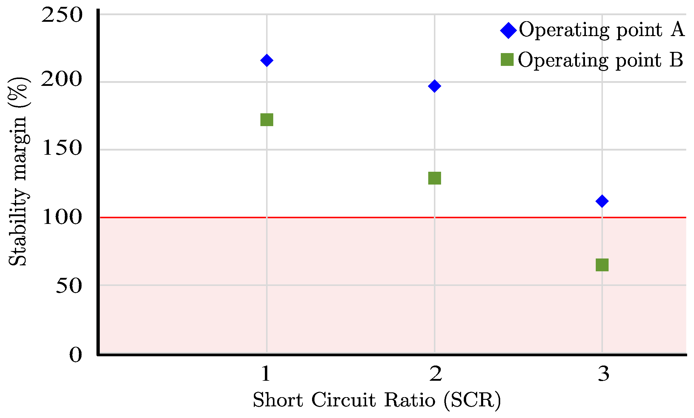
• Stability analysis of GFM converter-dominated grids using robust control theory is conducted by studying the stability margin for different operating conditions of the grid.
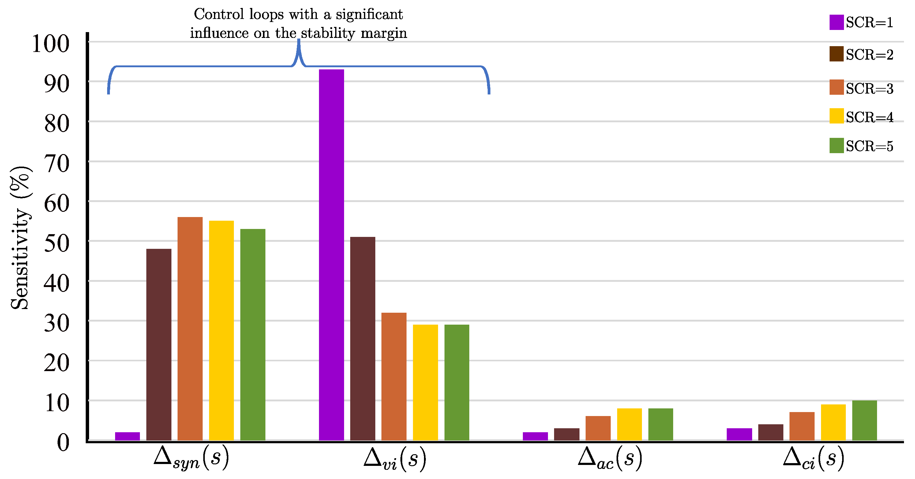
• Sensitivity analysis of the uncertain control loops is also investigated in order to determine which of the control loops have a significant impact on the stability of GFM converter-dominated grids.

This paper is organized as follows: In Section 2, the discussion and modelling of the generic GFM converter is illustrated in detail. In Section 3, the grey-box modelling of the GFM converters and the interconnection with power grid are discussed. In Section 4, the robust stability analysis of the grid considering a single GFM converter is presented. In Section 5, the HIL result is presented, and in Section 6 a brief conclusionis provided.

2. Power Converters Control System Uncertainties and Their Modelling

Making a few assumptions about the converters control system grounded in understanding of the physical laws governing power converters and their basic operation in power grids gives sufficient information to assume the converter as a grey-box rather than viewing it as a black-box model, which would be based solely on impedance-based measurements. For instance, manufacturing industries provide the mode of operations of the converters (e.g., GFL or GFM) and generic information about their control system as long as it does not reveal confidential details. In addition, the mathematical equations used in power converter models, like energy conservation and reference frame transformations, which are derived from fundamental principles of electromagnetism and standard mathematical techniques, are not protected by IP. With the generic information provided by the manufacturing industries without disclosing the internal details, the power converters can be modelled with uncertainty using the grey-box modelling approach.

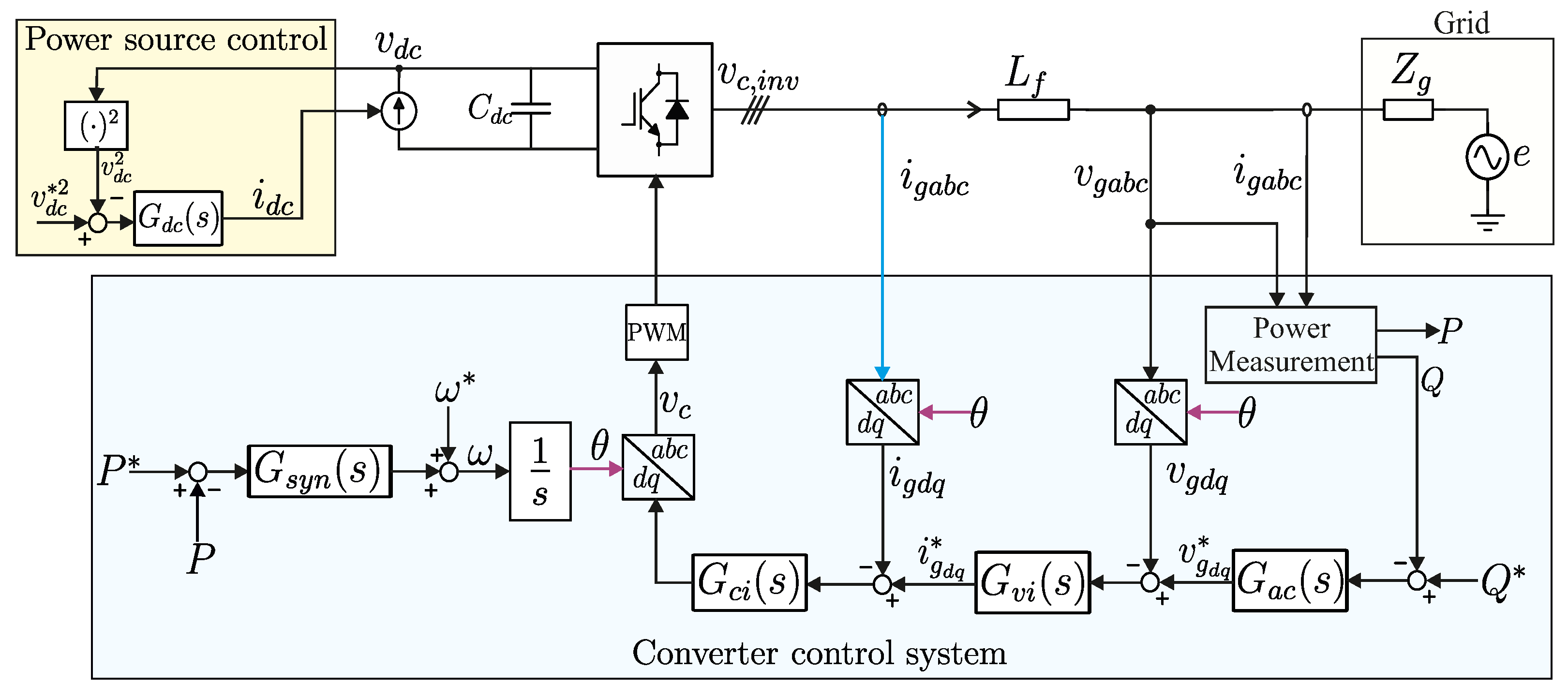
2.1. Generic Modelling of GFM Converters

In this paper, the generic GFM three-phase converter shown in Figure 1 is considered. The control structure of the generic GFM converter consists of a DC voltage control loop $G_{dc}\left(s\right)$, power synchronization loop $G_{syn}\left(s\right)$, the reactive power AC voltage loop $G_{ac}\left(s\right)$, the inner voltage loop $G_{vi}\left(s\right)$, and current loop $G_{ci}\left(s\right)$. Due to the possibility of implementing GFM converter control in various ways, the control loops inside the grey-box in Figure 1 are assumed to be unknown and they are modelled through unknown transfer functions $G_{syn}\left(s\right)$, $G_{ac}\left(s\right)$, $G_{vi}\left(s\right)$, and $G_{ci}\left(s\right)$. The DC voltage control loop is used to regulate the voltage at the power source, and it is assumed that the control tuning and its implementations are fully known.

The proper modeling of the converter considering its non-linearity is crucial to represent the operating point-dependent behaviors of the converter, which is necessary for system-level small-signal analysis.

2.1.1. Synchronization Loop Modelling

The generic representation of the synchronization loop in the GFM converter is an inclusive representation of all the possible synchronization mechanisms such as droop control [19], power synchronization control (PSC) [20], enhanced direct power control (EDPC), synchronverter [21], and synchronous power control (SPC) [22]. The virtual synchronous machine (VSM) swing equation is used to generically represent all the possible implementations of the GFM synchronization mechanisms. Therefore, the dynamic equation can be derived as follows:

$$\begin{array}{cc}\hfill \dot{\omega }& ={\displaystyle \frac{P^{*}-P_e}{J}}-{\displaystyle \frac{D_f\omega }{J}}\hfill \end{array}$$

(1)

$$\begin{array}{cc}\hfill \dot{\theta }& =\omega \hfill \end{array}$$

(2)

where J is the virtual inertia, $D_f$ is the damping coefficient, $P^{*}$ and $P_e$ are the reference active power and the converter active power output, respectively, and $\omega$ and $\theta$ are the angular frequency and the synchronization angle, respectively.

2.1.2. Reactive Power AC Voltage Loop Modelling

The reactive power injection profile of the grid is dependent on this loop and is designed based on the grid code requirement. Thus, a proportional (droop) controller is considered to generically model the reactive power AC voltage loop.

$$V{g}^{*}=\left[\begin{array}{c}{V}_n+K_p(Q^{*}-Q)\\ 0\end{array}\right]$$

(3)

where $V{g}^{*}$ and $V_n$ are the reference and nominal voltages, and Q and $Q^{*}$ the reactive power output of the converter and the reference reactive power.

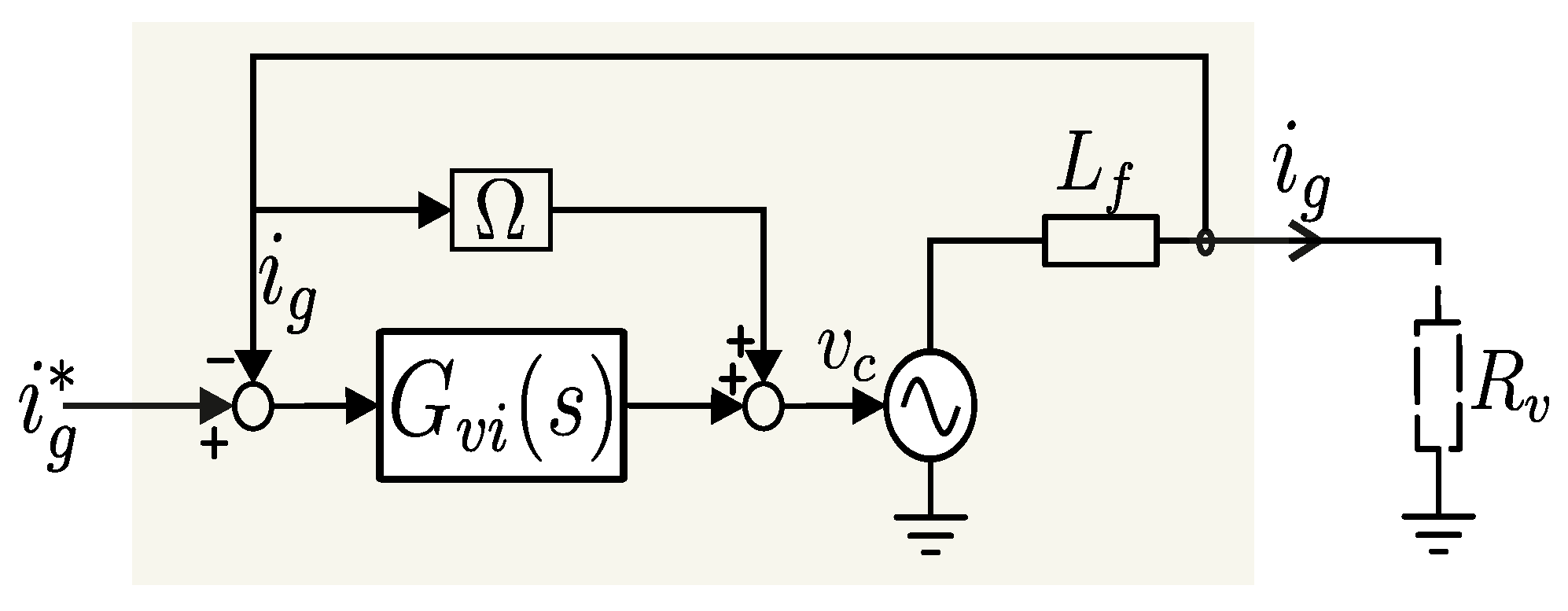
2.1.3. Cascaded Voltage and Current Control Loop Modelling

The integration of the voltage source converters (VSCs) subsystem to the distribution lines subsystem requires an accurate modelling of the inner voltage and current control loop. The cascaded loop is used to calculate the voltage for producing the pulse width modulation (PWM) signal of the converter.

A wide range of voltage control strategies were presented in [23] to manage and stabilize the output voltage of GFM converters. These schemes aim to ensure reliable voltage regulation and address various operational challenges. For the generic modelling of this loop, a cascaded proportional integral (PI) controller is considered.

The first control loop, which is used to adjust the reference current for the inner current loop, is based on the difference between the output voltage at the point of common coupling (PCC) and the reference voltage. The corresponding dynamic equation is provided in (5):

$$i_g^{*}=(K_{p_{vi}}+{\displaystyle \frac{K_{i_{vi}}}{s}})(V_g^{*}-V_g)$$

(4)

$$\begin{array}{c}\hfill i_g^{*}=K_{p_{vi}}(V_g^{*}-V_g)+K_{i_{vi}}{\Phi }_g\\ \hfill {\dot{\Phi }}_g=V_g^{*}-V_g\end{array}$$

(5)

where $i_g^{*}$ is the reference current of the current controller, ${\Phi }_g$ is the integral state voltage error, and $K_{p_{vi}}$ and $K_{i_{vi}}$ are the proportional and integral gains of the voltage controller.

The inner current control loop is modelled using the impedance modelling approach, as in [24], which permits the interconnection of VSCs and distribution lines without the need of a virtual resistor as shown in Figure 2 [25].

$$v_c-v_g=L_f{\displaystyle \frac{d{i}_g}{dt}}+L_f\Omega i_g$$

(6)

$$i_g={\displaystyle \frac{v_c-v_g}{L_f(s+\Omega )}}$$

(7)

$$v_c=(K_{p_{ci}}+{\displaystyle \frac{K_{i_{ci}}}{s}})(i_g^{*}-i_g)+L_f\Omega i_g$$

(8)

where $\Omega$ is the $dq$-axis decoupling term and $K_{p_{ci}}$ and $K_{i_{ci}}$ are the proportional and integral gains of the current controller.

By substituting (8) into (7), the impedance model of the VSC current control loop is derived, as presented in (9). A detailed discussion can be found in [25].

$$\begin{array}{c}\hfill G_c\left(s\right)={\displaystyle \frac{w_{cc}}{s+w_{cc}}}\\ \hfill Y_c\left(s\right)={\displaystyle \frac{s}{K_{p_{ci}}s+K_{i_{ci}}}}\end{array}$$

(9)

where ${\omega }_{cc}$ is the bandwidth of the current loop. The state space model of the current loop is realized using the non-physical state variables defined by $i_c=G_c\left(s\right)i_g^{*}$ and $v_{cc}={\displaystyle \frac{K_{i_{ci}}}{s}}(i_c-i_g)$.

$$\begin{array}{c}\hfill v_g=K_{p_{ci}}(i_c-i_g)+v_{cc}\\ \hfill {\dot{v}}_{cc}=K_{i_{ci}}{i}_c-K_{i_{ci}}{i}_g\\ \hfill {\dot{i}}_c=-w_{cc}{i}_c+w_{cc}{i}_g^{*}\end{array}$$

(10)

2.1.4. DC Voltage Control Loop Modelling

A Proportional–Integral (PI) controller is employed to regulate the DC input voltage of the GFM converter. The operation of the PI controller is based on the squared difference between the actual DC voltage and the desired DC voltage reference. By minimizing this difference, the PI controller adjusts the current ($i_{dc}$) from the energy sources (e.g., storage systems and wind turbine) to ensure that the DC voltage remains close to its set point. Therefore, the DC voltage control loop is modelled through the dynamic equations as follows:

$$i_{dc}=K_{p_{dc}}(V_{dc}^{*2}-V_{dc}^2)+K_{i_{dc}}{\Phi }_{dc}$$

(11)

$${\dot{\Phi }}_{dc}=V_{dc}^{*2}-V_{dc}^2$$

(12)

where ${\Phi }_{dc}$ is the integral state DC voltage error, and $K_{p_{dc}}$ and $K_{i_{dc}}$ are the Proportional and Integral gains of the DC voltage controller. The DC side of the converter dynamics is described by a non-linear power balance equation as in [25,26], by assuming that there is no conversion loss.

$$v_{dc}{i}_{dc}-c_{dc}{\displaystyle \frac{d{v}_{dc}}{dt}}{v}_{dc}={\displaystyle \frac{3}{2}}{v}_{gdq}^T{i}_{gdq}$$

(13)

$${\dot{v}}_{dc}=-{\displaystyle \frac{3}{2}}{\displaystyle \frac{1}{c_{dc}{v}_{dc}}}{v}_{gdq}^T{i}_{gdq}+{\displaystyle \frac{1}{c_{dc}}}{i}_{dc}$$

(14)

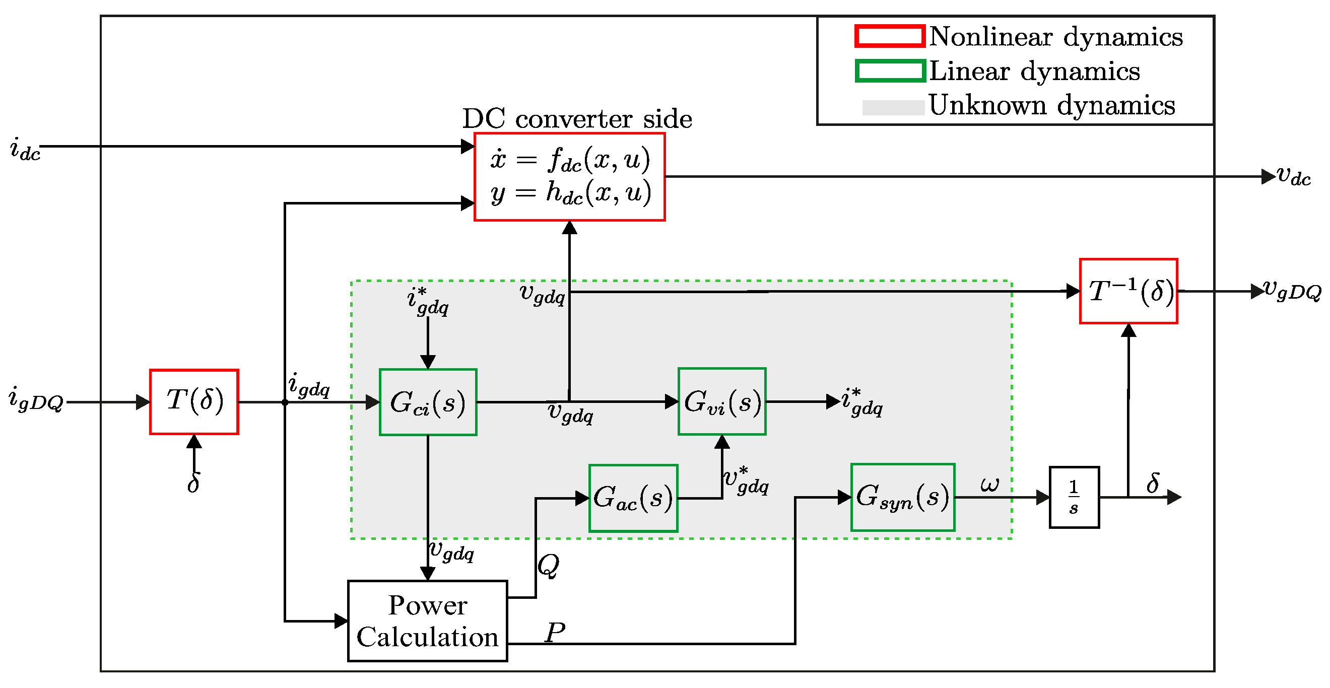
2.2. Grey-Box Non-Linear Modelling of GFM Converter

The grey-box modelling strategy of the GFM converter shown in Figure 1 is illustrated in Figure 3. The model in Figure 3 is composed of non-linear blocks (in red) and linear blocks (in green). The non-linear dynamics of the DC side of the converter and DC voltage control dynamics indicated in (11), (12), and (14) are assumed to be known without uncertainty by assuming that the DC link capacitor $C_{dc}$ and the control tunings for the PI controller are known.

The converter model in Figure 3 presents both input/output for the AC grid interconnection ($v_{g_{DQ}}$, $i_{g_{DQ}}$) and DC interconnection ($v_{dc}$, $i_{dc}$). In the cases of multiple parallel operations of grid-connected converters, which is shown in Figure 4, the frequency of each converter is determined by its local power sharing controller and is modelled using its own local reference frame [27,28]. Thus, the transformation of the voltages and currents from global to local frame and vice versa is performed by the non-linear blocks, the direct and inverse rotation matrices $T\left(\delta \right)$ and $T^{-1}\left(\delta \right)$. The matrix $T\left(\delta \right)$ is defined as follows:

$$T\left(\delta \right)=\left(\begin{array}{cc}cos\delta & sin\delta \\ -sin\delta & cos\delta \end{array}\right)$$

(15)

and used in the algebraic relations $i_{g_{dq}}$ = $T\left(\delta \right)$$i_{g_{DQ}}$ and $v_{g_{DQ}}$ = $T^{-1}\left(\delta \right)$$v_{g_{dq}}$. There is no uncertainty on the matrices $T\left(\delta \right)$ and $T^{-1}\left(\delta \right)$, which can thus be considered as known blocks in the converter model in Figure 3. The remaining blocks in Figure 3 are all linear: the integral relationship $\dot{\delta }=\omega$ is linear and certain, while the transfer functions $G_{syn}\left(s\right)$, $G_{ac}\left(s\right)$, $G_{vi}\left(s\right)$, and $G_{ci}\left(s\right)$ are linear but unknown.

The uncertain control systems of the converter indicated with a green dashed frame in Figure 3 can be modelled by applying frequency-dependent uncertainty to the generic representation of the respective control loops using the multiplicative uncertainty principle.

Frequency-dependent uncertainty refers to the uncertainty in a system’s behaviour or parameters that vary as a function of frequency. Applying this uncertainty type in the grey-box models of GFM converters helps to capture the essential dynamics of GFM converters across different frequency ranges. While this approach is effective for analysing different operational scenarios, its assumptions may not fully hold if the converter type or control structure is changed.

2.3. Multiplicative Uncertainty Formulation

According to the robust control theory to model the unknown subsystems, the amount of uncertainty of the subsystem must be properly quantified and mathematically characterized [29,30]. The uncertain converter control systems can be modelled by using either additive complex norm-bounded perturbations (additive uncertainty) or linear multiplicative perturbations which are defined in the frequency domain. Due to its simplicity in robust stability analysis and performance parameters calculation, multiplicative uncertainty modelling [29] is used in this paper. The multiplicative uncertainty is formulated as follows (16):

$$G_p\left(s\right)=G_n\left(s\right)(1+\omega \Delta \left(s\right));|\Delta \left(j\omega \right)|\le 1$$

(16)

where:

• $G_p\left(s\right)$ is the real plant transfer function.
• $G_n\left(s\right)$ is the transfer function of the nominal control loop implementations. In this case, the control loop parameters and implementations are totally unknown, so the nominal control loop $G_n\left(s\right)$ is chosen by the initial guess made with the generic knowledge about the converter.
• $\Delta \left(s\right)$ is the uncertainty transfer function for which the real plant $G_p\left(s\right)$ is deviated from the initial guess $G_n\left(s\right)$. For instance, if a higher deviation is expected in the real implementations of the control loop, then $\Delta \left(s\right)$ can be chosen as a high-pass filter. The unknown frequency-dependent transfer function $\Delta \left(s\right)$ can be defined using a MATLAB 2023b command $ultidyn\left(\right)$ with $H_{\infty }$ norm of unitary and $makeweight\left(\right)$ can be used to shape the frequency response of the uncertain function.
• $\omega$ is a scalar constant which quantifies the amount of uncertainty.

2.4. Quantitative Design of the Uncertainty in the Converter Control System

The multiplicative uncertainty formulation is now applied to all the uncertain control loops $G_{syn}\left(s\right)$, $G_{ac}\left(s\right)$, $G_{vi}\left(s\right)$, and $G_{ci}\left(s\right)$, as shown in Figure 3. The definition of the nominal transfer function $G_n\left(s\right)$ and the uncertainty $\omega \Delta \left(s\right)$ is conducted loop-by-loop, tailored to the individual characteristics and possible implementations of each specific loop.

To model the uncertainties of each control loop, lower uncertainty in low-frequency regions and high uncertainty in high-frequency regions were assumed. These assumptions were made based on the control system principles of grid-forming converters and power systems. High-frequency dynamics are highly influenced by fast-switching behaviours of the converters, unmodelled dynamics, and the interaction of high-bandwidth control loops, which are inherently more sensitive to parameter variations and external disturbances. Conversely, at low-frequency regions, dynamics are shaped by the interactions between voltage and frequency control loops and the grid’s steady-state properties. These low-frequency characteristics are less variable because they are governed by more stable physical parameters. It is also common practice in robust stability analysis to consider high uncertainties in high-frequency ranges to take in to account the unmodelled dynamics [29,30]. The quantification of the uncertainties depends on the specific loops, which is further discussed in the following subsections.

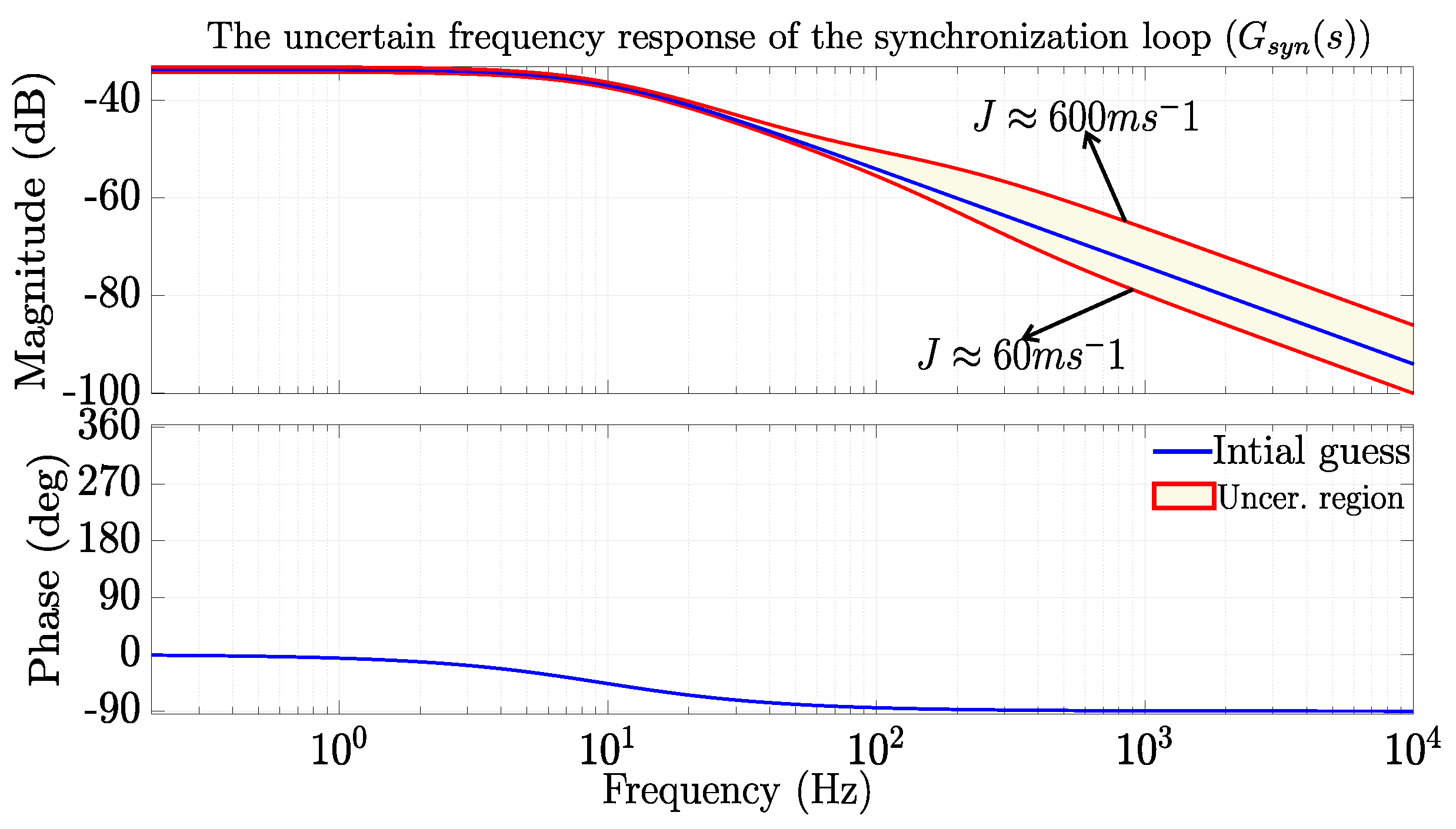
2.4.1. Synchronization Loop $G_{syn}\left(s\right)$

Various synchronization mechanisms for GFM converters were presented in different studies, including droop [19], power synchronization control (PSC) [20], enhanced direct power control (EDPC), synchronverter [21], and synchronous power control (SPC) [22]. The manufacturers generally kept the converters control system and their tunings confidential. In such cases, a nominal plant (i.e., initial guess) $G_{n_{syn}}\left(s\right)$ for the synchronization loop represented in grey colour in Figure 3 is firstly defined, and the unknown dynamics are then included through proper frequency-dependent uncertainty ${\omega }_{syn}{\Delta }_{syn}\left(s\right)$. So, as an initial guess $G_{n_{syn}}\left(s\right)$, the VSM swing equation is considered:

$$\begin{array}{c}\hfill \omega =G_{{}_{n}syn}\left(s\right)(P^{*}-P)\\ \hfill G_{{}_{n}syn}\left(s\right)={\displaystyle \frac{\frac{1}{J}}{s+\frac{D_f}{J}}}\end{array}$$

(17)

The uncertainty definition by means of ${\omega }_{syn}$ and ${\Delta }_{syn}$ must be conducted with several considerations, for the unknown real plant to represent all the possible synchronization loop implementations and their parameter tuning. The relations and equivalency of all those implementations are discussed in [23,31] by properly choosing their parameters. The representation of the synchronization mechanisms are highly different at high-frequency ranges so, it is reasonable to assume higher uncertainty at high-frequency ranges to be able to represent all of them. In the light of this, ${\omega }_{syn}$ is chosen 1.5 (150% uncertainty on the nominal plant $G_{{}_{n}syn}\left(s\right)$) and ${\Delta }_{syn}\left(s\right)$ is chosen to be low at low frequency and high at high frequency. Based on the assumptions made to consider all the possible synchronization loop implementations, the transfer function of the uncertainty is given by Equation (18).

$${\Delta }_{syn}\left(s\right)={\displaystyle \frac{s+{\tau }_{z_{syn}}}{s+{\tau }_{p_{syn}}}}$$

(18)

where ${\tau }_{z_{syn}}$ and ${\tau }_{p_{syn}}$ are chosen to give low uncertainty in the low-frequency range and high uncertainty in the high-frequency range. The resulting synchronization loop transfer function $G_{syn\left(s\right)}$ is shown in Figure 5. The blue curve in Figure 5 is the initial guess $G_{{}_{n}syn}\left(s\right)$ of the synchronization loop, while the yellow region in the Bode plot is the admissible region where the frequency response of the real implementation $G_{syn}\left(s\right)$ must lay.

2.4.2. Reactive Power AC Voltage Loop $G_{ac}\left(s\right)$

The AC voltage loop is more constrained to the grid reactive power requirement. With a proper knowledge of the grid code, it is reasonable to assume no uncertainty in the AC voltage loop in the low-frequency range, i.e., ${\Delta }_{ac}\left(s\right)=0$. At high-frequency ranges, the response of various controller implementations for AC voltage loop has to be considered. In this paper, the nominal AC voltage control loop is modelled with a proportional (droop) constant and known gain.

$$\begin{array}{c}\hfill V{g}^{*}=\left[\begin{array}{c}{V}_n+G_{n^{ac}}\left(s\right)(Q^{*}-Q)\\ 0\end{array}\right]\\ \hfill G_{n^{ac}}\left(s\right)=K_p\end{array}$$

(19)

With the addition of a high-frequency uncertainty, obtained by setting ${\omega }_{ac}=0.6$ and ${\Delta }_{ac}\left(s\right)$ as a high-pass filter. The resulting transfer function for the reactive power AC voltage loop uncertainty is given by (20) and the uncertain implementation of this control loop lays in the yellow region of the Bode plot shown in Figure 6.

$${\Delta }_{ac}\left(s\right)={\displaystyle \frac{s}{s+{\tau }_{p_{ac}}}}$$

(20)

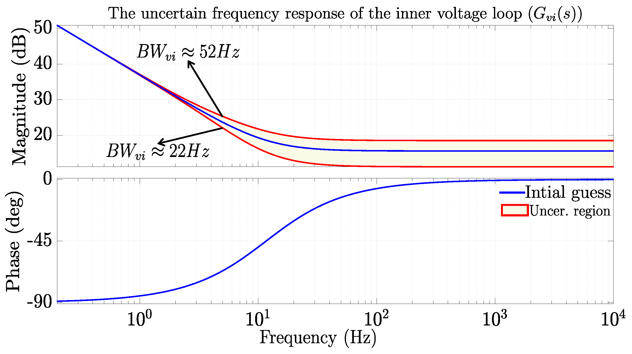
2.4.3. Inner Voltage Control Loop $G_{vi}\left(s\right)$

The primary function of this control loop is to support reactive power to the AC grid. It is therefore conceived to control the voltage $v_g$ to be as close as possible to the nominal value during grid faults, grid disturbances, and over currents. This control loop can be modelled using PI, PR, or virtual admittance models. To encompass all the possible implementations, higher uncertainty in the high-frequency range is considered. The nominal model is with a PI controller tuned with symmetrical optimum technique [26].

$$\begin{array}{c}\hfill i_g^{*}=G_{n_{vi}}\left(s\right)\ast \left(\begin{array}{c}{v}_g^{*}\\ v_g\end{array}\right)\\ \hfill G_{n_{vi}}\left(s\right)=K_{p_{vi}}+{\displaystyle \frac{K_{i_{vi}}}{s}}\end{array}$$

(21)

For the uncertain model, the uncertainty ${\Delta }_{vi}\left(s\right)$ is chosen as a high-pass filter without any uncertainty in the low-frequency range with the weighting constant ${\omega }_{vi}=0.4$. The resulting transfer function for the uncertainty is given by (22) and the uncertain transfer functions of the inner voltage loop implementations lays in the yellow region as depicted in Figure 7.

$${\Delta }_{vi}\left(s\right)={\displaystyle \frac{s}{s+{\tau }_{p_{vi}}}}$$

(22)

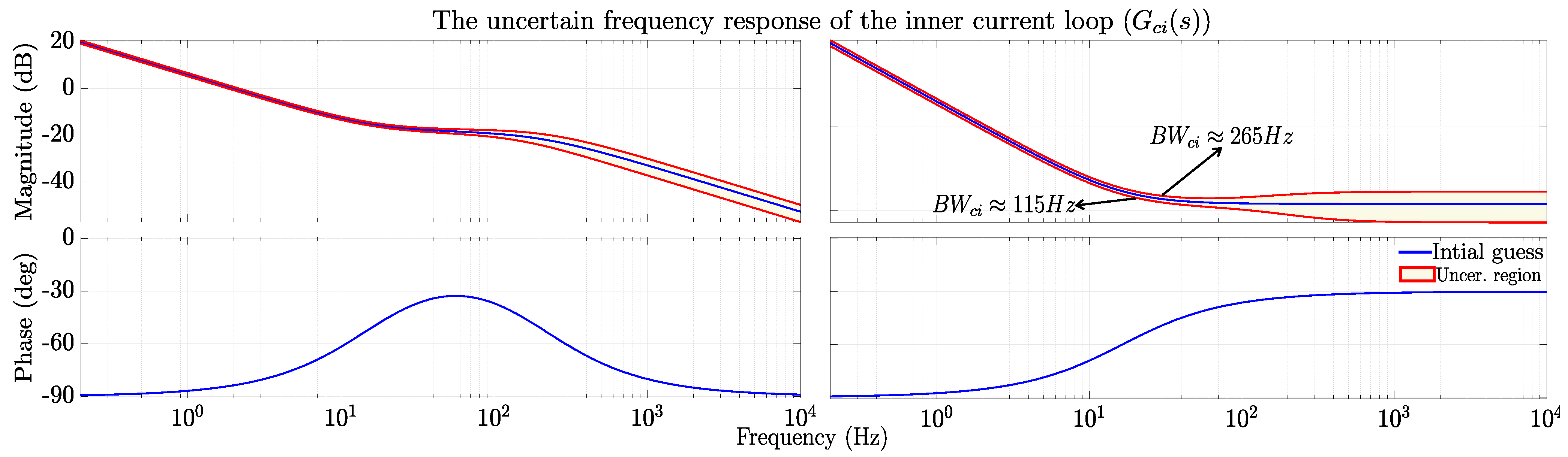
2.4.4. Inner Current Control Loop $G_{ci}\left(s\right)$

The inner loop is generally designed to have higher bandwidth than the outer loops in order to have a quick response to the change in the command signals. The implementation of this control loop is achieved by taking in to account the negative sequence and harmonic compensation schemes. Therefore, higher uncertainty in the high-frequency range and low uncertainty in the low-frequency range is considered. The generic implementation is a PI controller tuned with the technical optimum technique [26]. Therefore, it is modelled as a Multiple Input Multiple Output (MIMO) system as in (23)

$$\begin{array}{c}\hfill v_g=G_{n_{ci}}\left(s\right)\ast \left(\begin{array}{c}{i}_g^{*}\\ i_g\end{array}\right)\\ \hfill G_{n_{ci}}\left(s\right)=\left(\begin{array}{cc}{\displaystyle \frac{K_{p_{ci}}^{2}s+K_{p_{ci}}{K}_{i_{ci}}}{s^2{L}_f+K_{p_{ci}}s}}{I}_{2x2}& -(K_{p_{ci}}+{\displaystyle \frac{K_{i_{ci}}}{s}})I_{2x2}\end{array}\right)\end{array}$$

(23)

For the uncertain model, ${\Delta }_{ci}\left(s\right)$ is chosen as a high-pass filter with a slightly lower DC gain in the low-frequency range and the weighting constant ${\omega }_{ci}=0.4$. The resulting transfer function of the uncertainty is defined as a MIMO high-pass filter given by Equation (24).

$${\Delta }_{ci}\left(s\right)=\left(\begin{array}{cc}{\displaystyle \frac{s+{\tau }_{z_{ci}}}{s+{\tau }_{p_{ci}}}}& 0\\ 0& {\displaystyle \frac{s+{\tau }_{z_{ci}}}{s+{\tau }_{p_{ci}}}}\end{array}\right)$$

(24)

where ${\tau }_{z_{ci}}$ and ${\tau }_{p_{ci}}$ are chosen to give high uncertainty in the high-frequency range and low uncertainty in the low-frequency range. The uncertain transfer functions of the inner current loop implementations lays in the yellow region, as depicted in Figure 8.

2.4.5. DC Voltage Control Loop $G_{dc}\left(s\right)$

In this paper, the DC voltage control loop is used to control the voltage from the power source (storage system) and it is modelled without uncertainty, which means that ${\omega }_{dc}=0$ and the uncertainty ${\Delta }_{dc}\left(s\right)=0$.

$$\begin{array}{c}\hfill i_{dc}=G_{n_{dc}}\left(s\right)(V_{dc}^2-V_{dc}^{*2})\\ \hfill G_{n_{dc}}\left(s\right)=G_{p_{dc}}\left(s\right)=K_{p_{dc}}+{\displaystyle \frac{K_{i_{dc}}}{s}}\end{array}$$

(25)

The parameters representing the uncertainties of all control loops are chosen to account for variations in their implementation and to reflect a level of conservativeness that avoids making the grid system robustly stable for all possible grid conditions. Considering these factors, the parameters of $\Delta \left(s\right)$ for all uncertain control loops, which ensure robust stability under the specified grid conditions, have been determined and are reported in

Table 1. Parameters of the uncertainty $\Delta \left(s\right)$ able to ensure grid stability.

Control Loop	Parameters for Uncertainty
Synchronization loop	${\tau }_{z_{syn}}=22$, ${\tau }_{p_{syn}}=1080$
AC voltage loop	${\tau }_{p_{ac}}=1630$
Inner voltage loop	${\tau }_{p_{vi}}=33$
Inner current loop	${\tau }_{z_{ci}}=20$, ${\tau }_{p_{syn}}=1005$

.

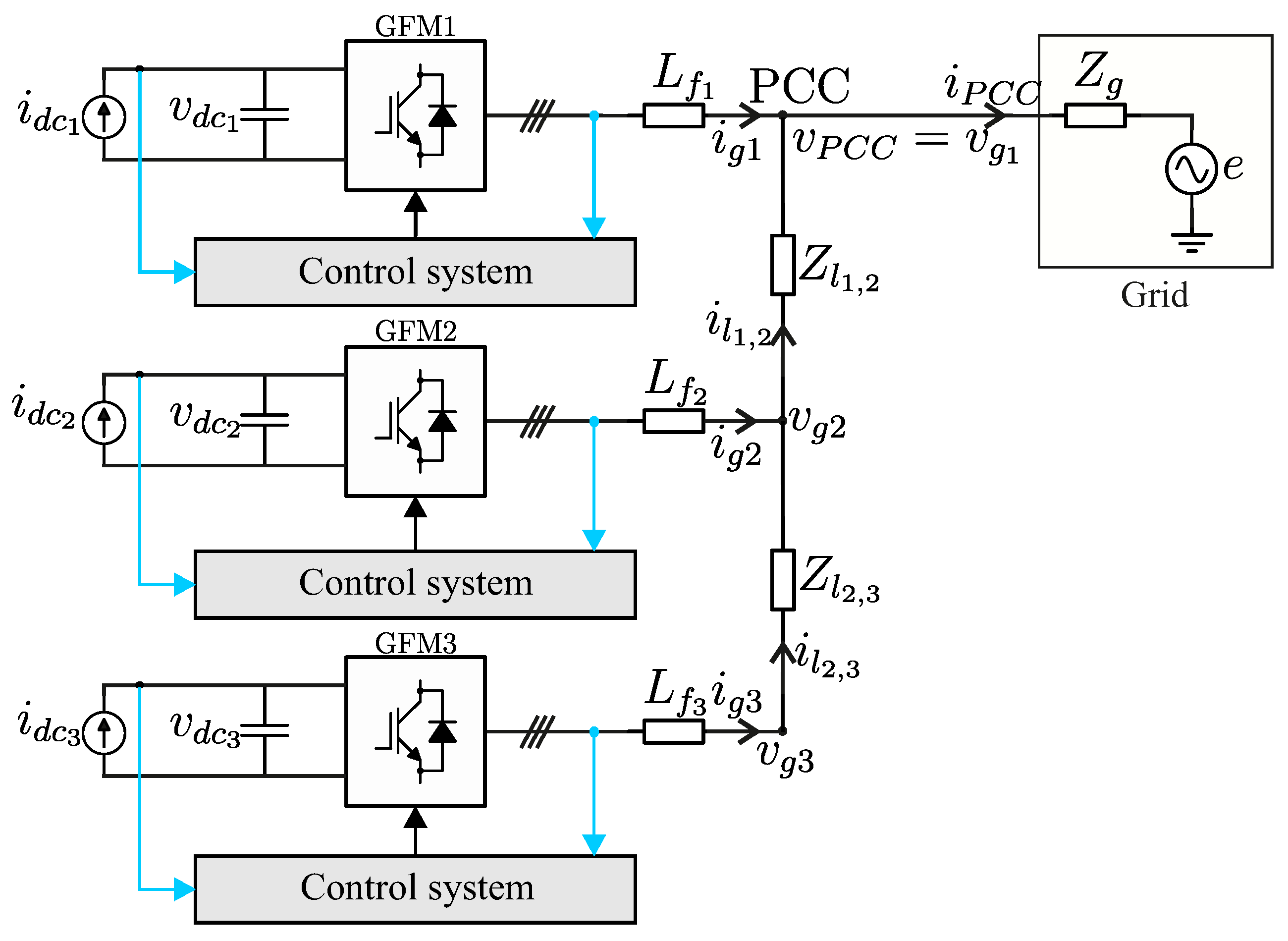
3. Non-Linear Grey-Box State-Space Model of Converter-Dominated Grids

The unknown model of the converter’s control system is simply the interconnection of the two blocks: nominal control system and the uncertainty of control systems, as shown in Figure 9. This approach is typically used in robust control theory [29,30] to incorporate multiplicative uncertainties in the form (16) by means of linear fractional transformation (LFT). The uncertainty of the control system shown in Figure 9 is defined as $7X7$ MIMO transfer matrix ${\omega }_{ctl}{\Delta }_{ctl}\left(s\right)$, which is the concatenation of the uncertainties of all control loops as defined in (26).

The remaining blocks of the converter model in Figure 3 that lay outside the dashed green rectangle (dc converter side, rotation matrices, and frequency/angle differential relationship) are embedded into the block known non-linear part, as shown in Figure 9 with red outline. The resulting converter model in Figure 9 is favourable for robust stability analysis, since the uncertainty of the control system is interconnected with a fully linear subsystem and the converter non-linear part is isolated and cannot be directly affected by the uncertainty. One of the key advantages of the converter model proposed in this paper is its capability to take in to account the converter non-linearities, which is not addressed in previous articles in the same area of interest [32,33].

$${\omega }_{ctl}{\Delta }_{ctl}\left(s\right)=\left(\begin{array}{cccc}{\omega }_{ci}{\Delta }_{ci}\left(s\right)& 0& 0& 0\\ 0& {\omega }_{vi}{\Delta }_{vi}\left(s\right)& 0& 0\\ 0& 0& {\omega }_{ac}{\Delta }_{ac}\left(s\right)& 0\\ 0& 0& 0& {\omega }_{syn}{\Delta }_{syn}\left(s\right)\end{array}\right)$$

(26)

Non-Linear Interconnection with the Power Grid

The non-linear DAE model of the grid is built according to the procedure in [25], and takes the following form:

$$\begin{array}{c}\hfill {\dot{x}}_{ps}=f_{ps}(x_{ps},u_{ps})\\ \hfill y_{ps}=h_{ps}(x_{ps},u_{ps})\end{array}$$

(27)

where $u_{ps}$ contains the grid voltage $E_g$, the reference power, and the DC voltage reference and $y_{ps}$ contains the variables used for the power flow analysis (voltage, angle, active, and reactive power of the converter).

The linearization of (27) requires the computation of the static equilibrium point $x_{pse}$ by solving through the Newton–Raphson method.

$$f_{ps}(x_{ps},u_{ps})=0$$

(28)

for a defined and constant input $u_{pse}$. The total uncertainty ${\Delta }_{ps}\left(s\right)$ does not play any role in the static converters and grid behaviour, but it influences only their transient dynamics. Thus, the uncertainty is considered null (${\Delta }_{ps}\left(s\right)=0$) in the non-linear static model (28) to compute the equilibrium point, and is then included in the grid model only after its linearization.

The computation of $x_{pse}$ through the solution of (28) with the standard Newton–Raphson method is a generalized power flow problem [34]. Once $x_{pse}$ is computed, the steady state power flow variables in $y_{ps}$ are obtained through the non-linear algebraic function $y_{pse}=h_{ps}(x_{pse},u_{pse})$. The resulting $y_{pse}$ for a single converter connected to the grid, as in Figure 1, is reported in

Table 2. Equilibrium point of the single converter under different SCRs and grid voltage $E_g$ steady state values.

${\mathit{E}}_{\mathit{g}}$	Steady State Var.	$\mathit{SCR}=1$	$\mathit{SCR}=2$	$\mathit{SCR}=3$	$\mathit{SCR}=4$
	$|v_g|$ (p.u.)	0.91	0.986	0.987	0.981
0.9	$\delta$ (deg)	39.79	15.42	10	7.41
	P (p.u.)	1	1	1	1
	Q (p.u.)	0.33	0.052	0.049	0.07
	$|v_g|$ (p.u.)	0.958	1.024	1.032	1.033
1	$\delta$ (deg)	32.7	14.02	9.17	6.83
	P (p.u.)	1	1	1	1
	Q (p.u.)	0.158	−0.089	−0.122	−0.125
	$|v_g|$ (p.u.)	0.993	1.06	1.08	1.088
1.1	$\delta$ (deg)	28.68	12.89	8.5	6.35
	P (p.u.)	1	1	1	1
	Q (p.u.)	0.027	−0.235	−0.30	−0.33

for different $SCR$ values and grid voltage levels $E_g$. The same fundamental steps used in the single-converter-based grid can be followed to extend the approach to a multiple-converter case.

RES-based power generation comprises various types of generation units which always show variability in their power generations due to their intermittent nature. A very flexible and comprehensive model which takes into account the differing dynamic behaviours and interactions among these units is highly needed to study the stability of the grid system. The stability of the grid is affected by the variation in power injected from the RESs due to the varying dynamic behaviours. The result presented in

Table 3. Power flow analysis under different grid operating points and short circuit ratio values.

Op. Point	Op. Point A			Op. Point B
Steady state var.	SCR = 1	SCR = 2	SCR = 3	SCR = 1	SCR = 2	SCR = 3
$|v_g|$ (p.u.)	0.958	1.024	1.032	0.93	1.03	1.04
$\delta$ (deg)	32.7	14.02	9.17	35.2	13.8	9.02
P (MW)	1	1	1	1.5	1.5	1.5
$Q\left(MVar\right)$	0.158	−0.089	−0.122	0.25	−0.12	−0.15

shows the effect of the variability of the RESs in power flow analysis with different power injections as different operating conditions, namely Operating Point A, with a 1 MW power injection from RESs, and Operating Point B, with a 1.5 MW power injection from RESs. However, the primary focus of this study is on the stability and dynamics of grid-forming converters within the grid, rather than the external environmental variability of RESs.

The model (27) is then linearized around the computed static equilibrium point based on the procedure in [25], obtaining:

$$\begin{array}{c}\hfill {\dot{X}}_{ps}=A_{ps}{X}_{ps}+B_{ps}{U}_{ps}\\ \hfill y_{ps}=C_{ps}{X}_{ps}+D_{ps}{U}_{ps}\end{array}$$

(29)

The linearized nominal system (29) is then expressed in a frequency domain as $G_{n_{ps}}$. The uncertain grey-box grid model can be then obtained by interconnecting the uncertainty ${\Delta }_{ps}\left(s\right)$ with the nominal grid model $G_{n_{ps}}$ using LFT, with the same procedure in [29], which is given by:

$$G_{ps}=G_{n_{ps},22}+G_{n_{ps},21}{\Delta }_{ps}{(I-G_{n_{ps},11}{\Delta }_{ps})}^{-1}{G}_{n_{ps},12}$$

(30)

with I identity matrix and $G_{n_{ps},ii}$, i = 1, 2 being the sub-blocks of $G_{n_{ps}}$.

4. Robust Stability Analysis

In this paper, structured singular value ($\mu$-analysis) is used to analyze the robust stability. $\mu$- analysis is a robust control tool that evaluates the smallest perturbation needed to destabilize a system with structured uncertainties. This approach is suitable for GFM converter-dominated grids, where structured uncertainties from variations in converter control implementations and unmodelled dynamics are common. Unlike traditional stability criteria, $\mu$- analysis explicitly incorporates these uncertainties, providing a more realistic and robust stability margin assessment.

The first step in robust stability analysis of the proposed system is the computation of the power grid stability margin ${\alpha }_{min}$ in the presence of grey-box converter models, which is defined as follows:

$${\alpha }_{min}:=\underset{{\Delta }_{ps}}{min}[\overline{\sigma }\left({\Delta }_{ps}\left(s\right)\right):det(I-G_{n_{ps},11}{\Delta }_{ps})=0]$$

(31)

being $\overline{\sigma }\left({\Delta }_{ps}\left(s\right)\right)$ the maximum singular value of ${\Delta }_{ps}\left(s\right)$, which belongs to the defined uncertainty set. The solution of (31) is computed through the command $robstab\left(\right)$ in MATLAB 2023b. The stability margin is inherently related to the choice of the uncertainty set and is generally more conservative compared with the results obtained by means of eigenvalue analysis. This is mainly because of the fact that the stability margin is calculated for a set of possible configurations instead of only for a specific one. However, it provides a mathematically accurate calculation of the robust stability of controls for MIMO systems [29,30].

However, if there are no uncertainties in the converter modelling, stability analysis using robust control theory is no longer used. One can use the linearized model to compute the eigenvalues of the system to analyze the stability of the grid-forming converter-dominated grid.

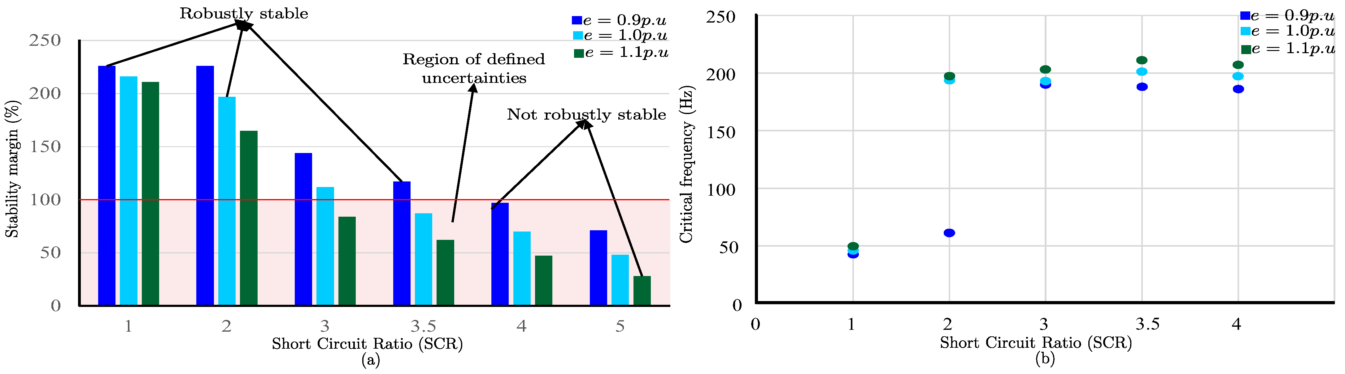
4.1. Robust Stability Analysis of the Grid with Single GFM Converter

The stability margin of the grid with the considered converter is obtained for different voltage levels under different SCR values, as depicted in Figure 10, by considering the parameters in

Table 4. Parameters considered for robust stability (RS) analysis.

Grid and Converter Parameters	Nominal Values	For RS Analysis
Line-to-line grid voltage (V)	690	690
Short Circuit Ratio	1.5	variable
R/X ratio	0.4	0.4
DC-link capacitor (mF)	22	22
Converters Control Parameters	Nominal Values	For RS Analysis
Active power reference $P^{*}$ (MW)	1	1
Switching frequency (kHz)	2	2
DC-link voltage reference (V)	1100	1100
DC voltage time constant (ms)	100	100
AC voltage controller gain	150 × 10−6	unknown
Bandwidth of the synchronization loop (rad/s)	540	unknown
Bandwidth of the inner voltage loop (rad/s)	460	unknown
Bandwidth of the inner current loop (rad/s)	1200	unknown

. In stability analysis, a higher stability margin signifies a greater ability of the system to maintain stability under varying conditions [29,30]. Therefore, the study of robust stability using stability margin follows the following rule:

Robust stability assessment criteria: In the context of control loop implementations considering multiplicative uncertainties, the studied system is robustly stable if the stability margin is beyond $100\%$ and conversely, if the stability margin is lower than $100\%$, then the system is not robustly stable.

This rule provides a clear benchmark for analysing the grid’s robust stability analysis with various scenarios. Applying this rule to the GFM converters-dominated power system is based on the stability margin values obtained and presented in Figure 10. Considering the case for $SCR=2$ and $e=1.0$ p.u., which has a stability margin of ${\alpha }_{min}=197\%$, indicates that the GFM converter-dominated grid is stable for all possible control tuning included by the uncertainty. This is because the smallest possible perturbation that is capable of destabilizing this converter-dominated grid system has an ${\mathrm{H}}_{\infty }$ norm of that is 197% of the maximum defined admissible perturbation, which implies that no destabilizing perturbation exists within the specified range of uncertainty. So, the GFM converter-dominated grid system is robustly stable for the considered case for all possible perturbations within the defined range of uncertainties.

For more illustrations, considering the system for a slightly increased SCR value (for instance, for $SCR=4$ with $e=1.0$ p.u.), the stability margin ${\alpha }_{min}=70\%$, which is lower than $100\%$. This implies that there is at least one destabilizing perturbation with an ${\mathrm{H}}_{\infty }$ norm greater than or equal to $70\%$ of the maximum permissible perturbation. Therefore, the system is not robustly stable, as there is at least one unstable control implementation within the specified range of uncertainty. Based on the results obtained, the GFM converter-dominated grids become not robustly stable for SCR values greater than $3.5$ due to their robust stability margin result below $100\%$.

As can be seen in Figure 10, the stability margin is decreasing with an increase in SCR values. This is because the increase in the SCR decreases the impedance of the grid which in turn reduces the damping effect provided by the grid. This causes the converter to become more sensitive to disturbances and variations in the grid voltage and frequency, leading to reduced stability margins. Due to the non-linearity of the converter model, for the same SCR value changing the grid voltage level affects the stability margin. As seen in Figure 10, the stability margin decreases with the increase in the grid voltage level. This is because the injection of reactive power which will increase the grid voltage reduces the stability margin of GFM converter-dominated grids. This dependability is because the change in the grid voltage level will also change the equilibrium points computed to linearize the system. Studying this dependency in the impedance-based black-box converter model is not possible.

The effect of different power injections from RESs on grid stability has been investigated under two operating conditions: Operating Point A, with a 1 MW power injection from RESs, and Operating Point B, with a 1.5 MW power injection from RESs. The result depicted in Figure 11 demonstrates that the stability margin decreases with higher power injection from the RESs. This indicates that increasing the power injected into the grid from RESs has a negative impact on stability. This suggests that the grid’s ability to maintain stability is sensitive to the level of power injected from RESs, requiring careful energy management and control strategies to mitigate stability issues.

Furthermore, the critical frequency value for which instability might occur in the system is also studied and computed through robust stability analysis tools for the scenarios considered for the simulation, and the result is presented in Figure 10. Considering the case $SCR=2$ and $e=0.9$ p.u., the critical frequency obtained from the simulation is 61 Hz. This implies the frequency at which instability might occur in the system for the considered case is at 61 Hz. Determining the critical frequency is very important to design the damping action without the full knowledge of the grid model during grid resonance instability.

4.2. Sensitivity Analysis of the Control Loops

The sensitivities of robust stability margins concerning each control loop uncertainties were analyzed in percentage to characterize how the variation in normalized perturbations of each control loop affects the grid stability margin. This analysis is necessary because it shows which control loops mainly affect overall system stability under uncertainties and gives insight into the influence of each control loop on the grid stability. The obtained results from the simulation of the model are presented in Figure 12 for different short circuit ratio values of the grid. For the considered cases, it is found that the reactive power AC voltage and the inner current loop design and tuning have less impact on the stability margin. On the other hand, the synchronization loop and the inner voltage loop tuning have a higher impact on the stability margin.

To prevent grid instability, system operators can use sensitivity analysis to develop and provide guidelines to converter manufacturers for tuning control loops [18]. These guidelines consist of specific tuning boundaries, derived using robust stability theory, which considers uncertainties and variations in grid conditions. By providing these boundaries, operators enable converters to operate within a safe range of parameters, maintaining stability even in the presence of disturbances or changing grid operating conditions.

5. Hardware-in-the-Loop (Hil) Results

In order to validate the robust stability analysis results obtained by robust control theory, the power grid in Figure 1 is simulated in a real-time simulation tool, the Typhoon HIL device. The validation of the generic model is firstly performed to verify whether it can exactly reflect the behaviours of GFM converters and followed by verification of robust stability analysis results.

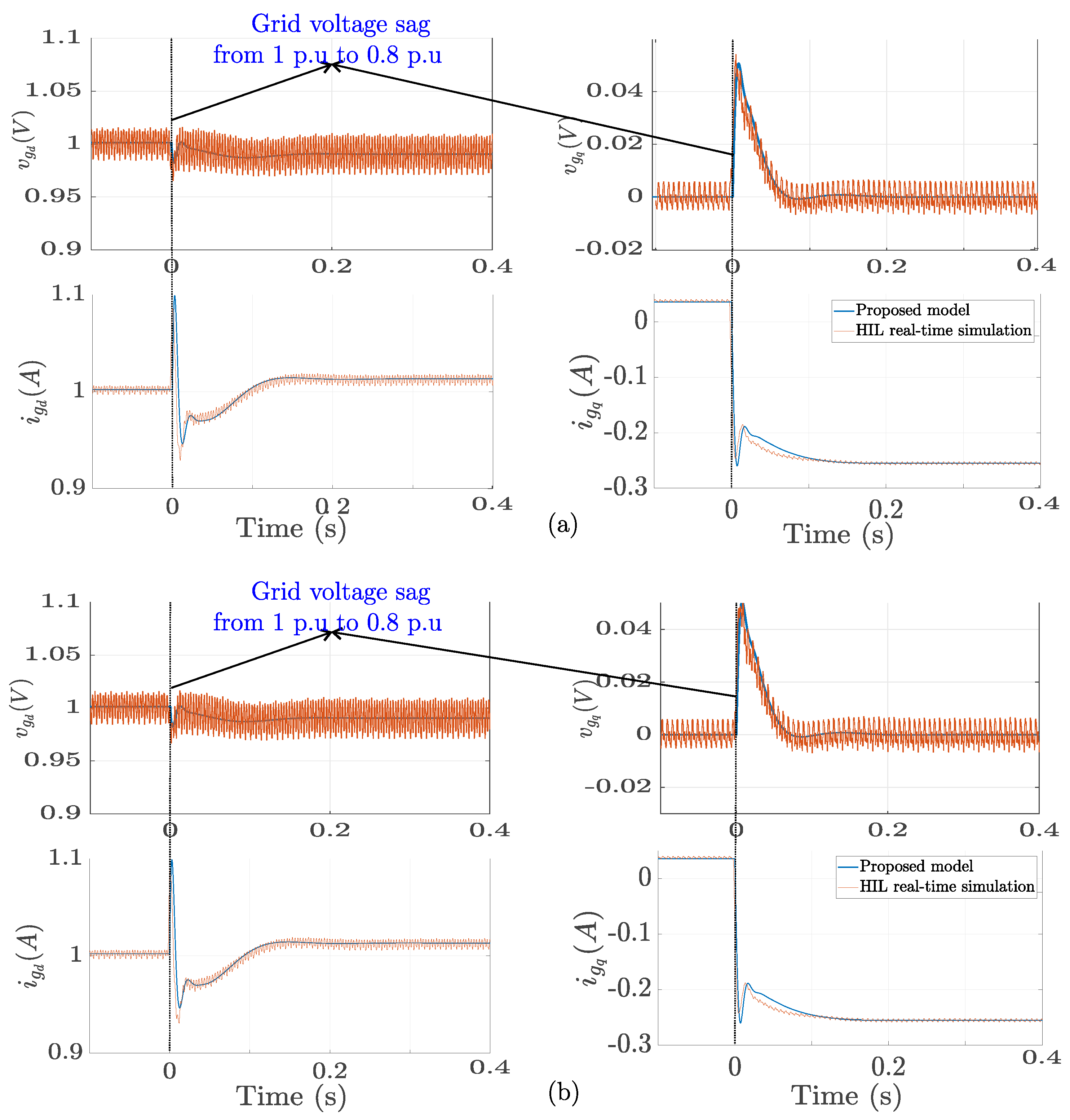
5.1. Model Validation with Hil Real Time Simulation

To ensure the accuracy of the results from the robust stability analysis, it is essential to verify that the mathematical model developed in Section 2 accurately reflects the behaviour of GFM converters. Due to the sense of generality of the model of the converter, the validation is performed with two control system implementations of GFM converters, i.e., Droop and VSM.

The dynamic response for each converter case is compared with the HIL result. As can be seen in Figure 13, during a voltage sag, the GFM converters attempt to compensate the drop by adjusting their output voltage, providing voltage support to prevent further sag. The current waveforms indicate that there is an increase in leading current to inject the necessary reactive power to the grid to compensate for the voltage drop and restore the voltage level and stability of the grid.

The results of the validation in Figure 13a,b confirm the accuracy of the proposed model for representing the control system implementations of GFM converters.

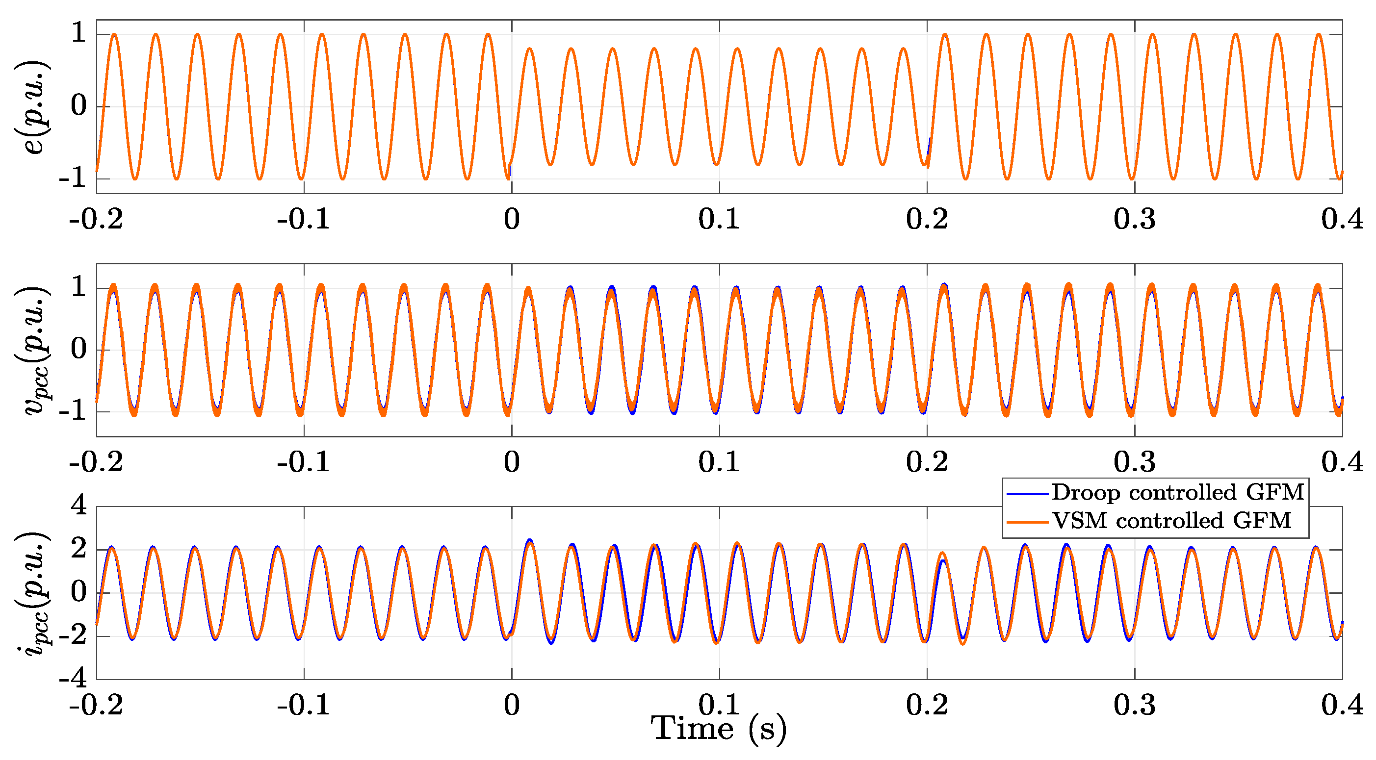
5.2. Robust Stability Analysis Validation

In order to validate the results obtained by the robust control theory, two converters with different control mechanisms are considered for the analysis: one utilizing VSM control and the other employing droop control. These control systems of the converters are accurately represented by the generic representation of the GFM in Section 2.

The result in Figure 14 is obtained by considering VSM-controlled GFM and droop-controlled GFM, with an SCR of 3.5. In this case, the grid is stable regardless of which converter cases are integrated with the grid. The grid is subjected to a voltage sag of 0.2 p.u. for 0.2 s, the stability is preserved even though a disturbance happens in the grid. This demonstrates that the grid to which the GFM converters are connected are stable for weak grid conditions regardless of the various possible control implementations.Differently, the result shown in Figure 15 is obtained by setting the SCR equal to 4.

As shown in the figure, the stability is preserved for droop-controlled GFM during transience, but instability is observed in the response of VSM-controlled GFM. This implies stability is not warranted for GFM converter-dominated grids when the SCR is greater than 3.5. Thus, based on the results from the robust stability analysis and the HIL implementation, the stability of weak grid is ensured when GFM converters are connected with it. Further increase in the short circuit ratio of the grid causes a stability problem. Therefore, robust stability of the grid to which GFM converters are connected is ensured for SCR values of 3.5 or lower, which aligns with the results obtained with robust control theory analysed by using the generic model discussed in Section 2.

To verify the sensitivity analysis result of which control loop tuning is playing a significant role in the stability of GFM converters-dominated grids, a real-time simulation is performed considering two tuning cases as defined in

Table 5. Control loop tunings for sensitivity analysis.

Control Systems	Initial Guess	Tuning A	Tuning B	Rationale for Selection
AC voltage controller gain	150 × 10−6	150 × 10−6	55 × 10−6	To study grid stability with a weak control for voltage regulation
Bandwidth of the inner current loop (rad/s)	1200	1200	445	To study grid stability with slowest current dynamics
Bandwidth of the synchronization loop (rad/s)	540	200	540	To study grid stability with low damping
Bandwidth of the inner voltage loop (rad/s)	460	170	460	To study grid stability with a slow response to the grid reactive power requirement

. The result in Figure 16 indicated by orange colour is obtained by using the case Tuning A, for which the synchronization and the inner voltage loop are tuned, while the reactive power AC voltage loop and the inner current loop remain unchanged from their initial settings. In this case, the stability of the grid is significantly distorted, underscoring the critical role of precise tuning in both the synchronization and inner voltage loops in the stability of the grid. Differently, the result indicated by green colour in Figure 16 demonstrates the second case, Tuning B, wherein the reactive power AC voltage loop and the inner current loop are tuned, and the synchronization and the inner voltage loop remain unchanged from their initial settings. In this case, the effect in the stability of the grid is insignificant, implying the reactive power AC voltage loop and the inner current loop tuning do not play a significant role in the stability of the GFM converters-dominated grids.

6. Conclusions

This paper presented a grey-box model of GFM converter without disclosing the internal details of the converter’s control system. Robust control theory is utilized to study the robust stability boundary of the grid with GFM converters connected to it. Based on the results obtained, the GFM converter-dominated grids are robustly stable for SCR values below 3.5. However, stability is not warranted for SCR values exceeding 3.5, as the stability margin is below $100\%$ for large SCR values. In addition, sensitivity analysis of the control loops is also conducted to give an intuition on which control loop tuning is playing a significant role in the stability of GFM converter-dominated grids. To demonstrate this, the bandwidths of the synchronization and the inner voltage loop, and the reactive power AC voltage loop and inner current loop, are reduced to below $40\%$ of their nominal value alternatively. It was found that the synchronization and the inner voltage loop significantly affect the stability of the grid, while the tuning of the reactive power AC voltage loop and inner current loop have a negligible effect on grid stability. Therefore, from control loop tuning’s point of view, to avoid grid instability, with this modelling approach, system operators can compute and deliver stability specifications to converter manufacturers in the form of a set of tuning boundaries for the control loops that ensures grid stability. In order to verify the results, a real-time simulation with Typhoon HIL is performed and it was demonstrated that the results in both MATLAB 2023b and HIL simulations are consistent.

References

1. Pishbahar, H.; Blaabjerg, F.; Saboori, H. Emerging grid-forming power converters for renewable energy and storage resources integration—A review. Sustain. Energy Technol. Assessments 2023, 60, 103538. [Google Scholar] [CrossRef]
2. Zhang, H.; Xiang, W.; Lin, W.; Wen, J. Grid Forming Converters in Renewable Energy Sources Dominated Power Grid: Control Strategy, Stability, Application, and Challenges. J. Mod. Power Syst. Clean Energy 2021, 9, 1239–1256. [Google Scholar] [CrossRef]
3. Liao, Y.; Wu, H.; Wang, X.; Ndreko, M.; Dimitrovski, R.; Winter, W. Stability and Sensitivity Analysis of Multi-Vendor, Multi-Terminal HVDC Systems. IEEE Open J. Power Electron. 2023, 4, 52–66. [Google Scholar] [CrossRef]
4. Arévalo-Soler, J.; Nahalparvari, M.; Groß, D.; Prieto-Araujo, E.; Norrga, S.; Gomis-Bellmunt, O. Small-Signal Stability and Hardware Validation of Dual-Port Grid-Forming Interconnecting Power Converters in Hybrid AC/DC Grids. IEEE J. Emerg. Sel. Top. Power Electron. 2024. [Google Scholar] [CrossRef]
5. Navarro-Rodríguez, Á.; García, P.; Gómez-Aleixandre, C.; Blanco, C. Cooperative Primary Control of a Hybrid AC/DC Microgrid Based on AC/DC Virtual Generators. IEEE Trans. Energy Convers. 2022, 37, 2837–2850. [Google Scholar] [CrossRef]
6. Hu, P.; Li, Y.; Yu, Y.; Blaabjerg, F. Inertia estimation of renewable-energy-dominated power system. Renew. Sustain. Energy Rev. 2023, 183, 113481. [Google Scholar] [CrossRef]
7. Saha, S.; Saleem, M.I.; Roy, T.K. Impact of high penetration of renewable energy sources on grid frequency behaviour. Int. J. Electr. Power Energy Syst. 2023, 145, 108701. [Google Scholar] [CrossRef]
8. Mehrasa, M.; Pouresmaeil, E.; Sepehr, A.; Pournazarian, B.; Catalão, J.P.S. Control of power electronics-based synchronous generator for the integration of renewable energies into the power grid. Int. J. Electr. Power Energy Syst. 2019, 111, 300–314. [Google Scholar] [CrossRef]
9. Liao, Y.; Li, Y.; Chen, M.; Nordstr, L.; Wang, X.; Mittal, P.; Poor, H.V. Neural network design for impedance modeling of power electronic systems based on latent features. IEEE Trans. Neural Netw. Learn. Syst. 2023, 35, 5968–5980. [Google Scholar] [CrossRef] [PubMed]
10. Suryani, A.; Sulaeman, I.; Rosyid, O.A.; Moonen, N.; Popović, J. Interoperability in Microgrids to Improve Energy Access: A Systematic Review. IEEE Access 2024, 12, 64267–64284. [Google Scholar] [CrossRef]
11. Paolone, M.; Gaunt, T.; Guillaud, X.; Liserre, M.; Meliopoulos, S.; Monti, A.; Van Cutsem, T.; Vittal, V.; Vournas, C. Fundamentals of power systems modelling in the presence of converter interfaced generation. Electr. Power Syst. Res. 2020, 189, 106811. [Google Scholar] [CrossRef]
12. Rasheduzzaman, M.; Mueller, J.A.; Kimball, J.W. Reduced-order small-signal model of microgrid systems. IEEE Trans. Sustain. Energy 2015, 6, 1292–1305. [Google Scholar] [CrossRef]
13. Lai, N.B.; Baltas, G.N.; Rodriguez, P. Small-Signal Modeling of Grid-Forming Power Converter. In Proceedings of the 2022 IEEE 13th International Symposium on Power Electronics for Distributed Generation Systems (PEDG), Kiel, Germany, 26–29 June 2022; pp. 1–5. [Google Scholar] [CrossRef]
14. Bryant, J.S.; McGrath, B.; Meegahapola, L.; Sokolowski, P. Small-Signal Modeling and Stability Analysis of a Droop-Controlled Grid-Forming Inverter. In Proceedings of the 2022 IEEE Power & Energy Society General Meeting (PESGM), Denver, CO, USA, 17–21 July 2022; pp. 1–5. [Google Scholar] [CrossRef]
15. Wen, B.; Boroyevich, D.; Mattavelli, P.; Burgos, R.; Shen, Z. Impedance-based analysis of grid-synchronization stability for three-phase paralleled converters. In Proceedings of the 2014 IEEE Applied Power Electronics Conference and Exposition—APEC 2014, Fort Worth, TX, USA, 16–20 March 2014; pp. 1233–1239. [Google Scholar] [CrossRef]
16. Sun, J. Impedance-Based Stability Criterion for Grid Connected Inverters. IEEE Trans. Power Electron. 2011, 26, 3075–3078. [Google Scholar] [CrossRef]
17. Riccobono, A.; Mirz, M.; Monti, A. Noninvasive online parametric identification of three-phase ac power impedances to assess the stability of grid-tied power electronic inverters in lv networks. IEEE J. Emerg. Sel. Top. Power Electron. 2018, 6, 629–647. [Google Scholar] [CrossRef]
18. Cecati, F.; Liserre, M. Interoperability Specifications for Multi Vendor Converter-Dominated Grid: A Robust Stability Perspective. TechRxiv 2024. [Google Scholar] [CrossRef]
19. Fazal, S.; Haque, M.E.; Arif, M.T.; Gargoom, A. Droop control techniques for grid forming inverter. In Proceedings of the 2022 IEEE PES 14th Asia-Pacific Power and Energy Engineering Conference (APPEEC), Melbourne, Australia, 20–23 November 2022; pp. 1–6. [Google Scholar]
20. Zhang, L.; Harnefors, L.; Nee, H.-P. Power-Synchronization Control of Grid Connected Voltage-Source Converters. IEEE Trans. Power Syst. 2010, 25, 809–820. [Google Scholar] [CrossRef]
21. Zhong, Q.-C.; Nguyen, P.-L.; Ma, Z.; Sheng, W. Self-synchronized synchronverters: Inverters without a dedicated synchronization unit. IEEE Trans. Power Electron. 2013, 29, 617–630. [Google Scholar] [CrossRef]
22. Rodríguez, P.; Citro, C.; Candela, J.I.; Rocabert, J.; Luna, A. Flexible Grid Connection and Islanding of SPC-Based PV Power Converters. IEEE Trans. Ind. Appl. 2018, 54, 2690–2702. [Google Scholar] [CrossRef]
23. Rosso, R.; Wang, X.; Liserre, M.; Lu, X.; Engelken, S. Grid-Forming Converters: Control Approaches, Grid-Synchronization, and Future Trends—A Review. IEEE Open J. Ind. Appl. 2021, 2, 93–109. [Google Scholar] [CrossRef]
24. Cecati, F.; Zhu, R.; Liserre, M.; Wang, X. State-feedback-based Low-Frequency Active Damping for VSC Operating in Weak-Grid Conditions. In Proceedings of the 2020 IEEE Energy Conversion Congress and Exposition (ECCE), Detroit, MI, USA, 11–15 October 2020; pp. 4762–4767. [Google Scholar] [CrossRef]
25. Cecati, F.; Zhu, R.; Liserre, M.; Wang, X. Nonlinear Modular State-Space Modeling of Power-Electronics-Based Power Systems. IEEE Trans. Power Electron. 2022, 37, 6102–6115. [Google Scholar] [CrossRef]
26. Teodorescu, R.; Liserre, M.; Rodriguez, P. Grid Converters for Photovoltaic and Wind Power Systems; John Wiley & Sons: Hoboken, NJ, USA, 2011. [Google Scholar]
27. Pogaku, N.; Prodanovic, M.; Green, T.C. Modeling, analysis and testing of autonomous operation of an inverter-based microgrid. IEEE Trans. Power Electron. 2007, 22, 613–625. [Google Scholar] [CrossRef]
28. Cavazzana, F.; Caldognetto, T.; Mattavelli, P.; Corradin, M.; Toigo, I. Analysis of Current Control Interaction of Multiple Parallel Grid Connected Inverters. IEEE Trans. Sustain. Energy 2018, 9, 1740–1749. [Google Scholar] [CrossRef]
29. Zhou, K.; Doyle, J.C. Essentials of Robust Control; Prentice Hall: Upper Saddle River, NJ, USA, 1998; Volume 104. [Google Scholar]
30. Skogestad, S.; Postlethwaite, I. Multivariable Feedback Control: Analysis and Design; John Wiley & Sons: Hoboken, NJ, USA, 2005. [Google Scholar]
31. D’Arco, S.; Suul, J.A. Equivalence of virtual synchronous machines and frequency droops for converter-based microgrids. IEEE Trans. Smart Grid 2013, 5, 394–395. [Google Scholar] [CrossRef]
32. Gao, X.; Zhou, D.; Anvari-Moghaddam, A.; Blaabjerg, F. Stability Analysis of Grid Following and Grid-Forming Converters Based on State-Space Model. In Proceedings of the 2022 International Power Electronics Conference (IPEC-Himeji 2022- ECCE Asia), Himeji, Japan, 15–19 May 2022; pp. 422–428. [Google Scholar] [CrossRef]
33. Li, C.; Huang, Y.; Wang, Y.; Monti, A.; Wang, Z.; Zhong, W. Modelling and small signal stability for islanded microgrids with hybrid grid-forming sources based on converters and synchronous machines. Int. J. Electr. Power Energy Syst. 2024, 157, 109831. [Google Scholar] [CrossRef]
34. Milano, F. An open source power system analysis toolbox. IEEE Trans. Power Syst. 2005, 20, 1199–1206. [Google Scholar] [CrossRef]
Figure 1. Generic representation of GFM converter with power synchronization loop, reactive power AC voltage loop, inner voltage loop, and current loop.
Energies 18 00587 g001
Figure 2. Current loop modelling.
Energies 18 00587 g002
Figure 3. The proposed modelling scheme for the generic GFM converter including linear, non-linear, and uncertain blocks.
Energies 18 00587 g003
Figure 4. The power grid consists of three grid-forming converters in parallel, with an unknown control systems.
Energies 18 00587 g004
Figure 5. The uncertain frequency response of the synchronization loop.
Energies 18 00587 g005
Figure 6. The uncertain frequency response of the reactive power AC voltage loop.
Energies 18 00587 g006
Figure 7. The uncertain frequency response of the inner voltage loop.
Energies 18 00587 g007
Figure 8. The uncertain frequency response of the inner current loop.
Energies 18 00587 g008
Figure 9. The block interconnection procedure to embed the uncertainty in the proposed grey-box non-linear converter model.
Energies 18 00587 g009
Figure 10. Robust stability analysis results for different SCR and grid voltage values: (a) Stability margin and (b) Critical frequency.
Energies 18 00587 g010
Figure 11. Grid stability margin with different power injections from RESs.
Energies 18 00587 g011
Figure 12. The sensitivity of the robust stability margin with respect to the individual control loops uncertainty.
Energies 18 00587 g012
Figure 13. The validation of the proposed GFM converter model with respect to: (a) Droop-controlled GFM converter and (b) VSM-controlled GFM converter.
Energies 18 00587 g013
Figure 14. The real-time HIL simulation of the grid connected to GFM converter of different control systems with S C R = 3.5 .
Energies 18 00587 g014
Figure 15. The real-time HIL simulation of the grid connected to GFM converter of different control systems with S C R = 4 .
Energies 18 00587 g015
Figure 16. The real-time HIL simulation of the grid with different control loop tunings: the response of Tuning A is indicated by orange colour and Tuning B is indicated by green colour.
Energies 18 00587 g016