Robust Optimal Dispatch of Microgrid Considering Flexible Demand-Side

Abstract

Objective To address the uncertainty in power grid scheduling caused by the output variability of distributed energy resources (DERs) in microgrids, as well as the limitations of stochastic optimization relying on accurate probability distributions and the overly conservative nature of robust optimization leading to insufficient economic performance, this paper proposes a disseminated robust optimization method for microgrid operation that considers flexible demand-side resources. Methods First, to address the uncertainty in the forecasting of wind and solar power scenarios, this paper launches a two-stage distributionally robust optimization (DRO) model based on a Kullback–Leibler (KL) divergence ambiguity set using a min–max–min framework. Then, the Column-and-Constraint Generation (C&CG) algorithm is employed to decouple the model for an iterative solution. Finally, simulation case studies are directed to validate the effectiveness of the proposed model. Results The demand response-based optimization model projected in the paper effectively enhances the flexibility of the Microgrid. Compared to robust optimization, this model reduces the daily operating cost by 2.86%. Although the cost is slightly higher (4.88%) than that of stochastic optimization, it achieves a balance between economy and robustness by optimizing the expected value under the worst-case probability distribution.

1. Introduction

In recent years, as environmental and energy issues have become increasingly critical, the exploration and utilization of renewable energy have garnered growing attention worldwide [1]. According to the latest statistics, China has ranked first globally in installed capacities of wind power and photovoltaics for multiple consecutive years [2]. With the rapid growth in renewable energy integration, the instability and uncertainty of wind power and photovoltaic power production have intensified, posing significant challenges to the safe and steady process of grid dispatch. Microgrids can efficiently coordinate equipment operation and interact compatibly with upper-level systems, demonstrating favorable characteristics for renewable energy integration. With the integration of demand-side response and electric vehicle loads, microgrid operation has become more complex. Ensuring its safe, economic, and environmentally friendly operation is a key focus for future development. The economic scheduling issue of the Microgrid is to diminish operating costs as much as possible and achieve efficient energy utilization [3,4].

The methodologies for addressing uncertainties in microgrid scheduling have evolved along distinct paradigms. A significant stream of research relies on Stochastic Optimization (SO), which utilizes predefined probability distributions to model uncertainties. For instance, reference [5] proposed a scenario-based stochastic scheduling model solved via rolling horizon optimization. This approach was extended by [6] to a multi-scenario, multi-timescale framework for AC-DC hybrid microgrids, and by [7] for scheduling multi-form microgrid clusters. Beyond scheduling, ref. [8] applied SO to a joint bidding problem for wind and storage. The common strength of these methods is their ability to leverage distributional information to seek cost-effective solutions. However, a critical limitation is their heavy reliance on accurate probability distributions, which are difficult to obtain in practice. When the actual distribution deviates from the estimated one, SO models can become over-optimistic and lack robustness.

In contrast, Robust Optimization (RO) methods make no assumptions about probability distributions, instead optimizing against the worst-case realization within an uncertainty set. Reference [9] established a foundational two-stage RO model for microgrids, a framework later enhanced by [10] through an advanced algorithm to improve computational efficiency. Literature [11] further refined the RO approach with a three-level min–max–min structure to derive more precise scheduling strategies. The primary advantage of RO is its rigorous, distribution-free guarantee of feasibility and reliability under all possible uncertainties. Nevertheless, this very strength leads to its main drawback: over-conservatism. By focusing solely on the worst-case scenario, which may have a very low probability, RO often sacrifices economic performance, resulting in high operating costs.

To bridge the gap between the economy of SO and the robustness of RO, Distributionally Robust Optimization (DRO) has emerged as a promising paradigm. DRO acknowledges that some distributional information is available but accounts for its ambiguity by optimizing over a set of plausible distributions (an ambiguity set). Studies on collaborative optimization [12] and peer-to-peer trading [13] have demonstrated its balanced approach. Applied to problems like chance-constrained management [14], DRO hedges against distributional errors without being overly pessimistic. To overcome the shortcomings of stochastic optimization’s reliance on probability distributions and the conservativeness of robust optimization, distributionally robust optimization (DRO) integrates the strengths of both. By optimizing the expected value under the worst-case probability distribution, it attains a relative equilibrium between robustness and financial efficacy.

Despite its promise, key research gaps remain in the application of DRO to integrated microgrid scheduling. Specifically, many existing studies lack a coordinated framework that simultaneously models the uncertainty of renewables and the flexibility of diverse demand-side resources—such as electric vehicle clusters, shiftable loads, and interruptible loads—within a computationally tractable DRO model. Furthermore, efficiently solving the resulting complex multi-level optimization problem remains a practical challenge.

To address the intermittency and randomness of wind and solar outputs, causing uncertainties in the Microgrid, as well as the problems that stochastic optimization depends on exact probability distributions, and robust optimization produces overly conservative scheduling results. Accordingly, this paper first constructs a probability distribution ambiguity set based on the KL Divergence to characterize the distribution range of uncertain parameters. Then, aiming to minimize the power exchange cost between the Microgrid and the distribution system, the operational cost of electric vehicles, and the wind and solar curtailment cost, a three-layer, two-stage min–max–min structured distributionally robust optimization model is developed. The framework comprises two main stages: the first stage performs deterministic planning for microgrid energy trading decisions, energy storage scheduling, and the charging and discharging power of electric vehicle fleets. In the second stage, based on the actual realization of uncertainty parameters, the optimal real-time scheduling strategy for the Microgrid is generated. To address the computational complexity of such multi-level nested optimization problems, the column-and-constraint generation (C&CG) algorithm is introduced. By decomposing the original three-level structure into a coupled system of the master difficulty and the Subproblem, the global ideal result is obtained through an iterative optimization approach.

Compared to existing research, the main contributions of this paper are threefold:

• A three-level min–max–min DRO framework integrating flexible demand-side resources. This structure uniquely embeds the search for the worst-case probability distribution within the optimization process, bridging the economic focus of stochastic optimization and the robustness of traditional robust optimization without relying on accurate probability distributions or being overly conservative.
• An ambiguity set for renewable generation based on KL divergence, with a clear interpretation of the risk parameter ρ. Chosen for its computational practicality, the KL divergence allows the model to handle distributional uncertainty. The parameter ρ serves as an adjustable risk-aversion lever, enabling decision-makers to balance economy and robustness based on data availability and risk preference.
• A coordinated microgrid scheduling model for EV clusters and adjustable loads, solved efficiently. The model aggregates EVs as a dispatchable unit and coordinates them with shiftable and interruptible loads. The complex three-level problem is effectively solved using the C&CG algorithm, ensuring computational feasibility for practical dispatch systems.

2. Microgrid System Architecture and Optimal Operation Model

Figure 1 illustrates a typical microgrid system architecture, whose core consists of dispersed new energy production units, energy storage strategies, composite loads, and a microgrid control center. The load side includes flexible adjustable loads (household appliances, air conditioners, electric vehicle charging stations) and conventional loads: the former are dynamically regulated through demand response by the control center, while the latter ensure power supply stability. The Microgrid flexibly adjusts the electricity consumption of flexible loads through time-of-use electricity pricing and compensation policies, thereby reducing operating costs, incentivizing load participation in demand response, and providing economic benefits to users.

2.1. Two-Stage Distributionally Robust Optimization Model for Microgrid

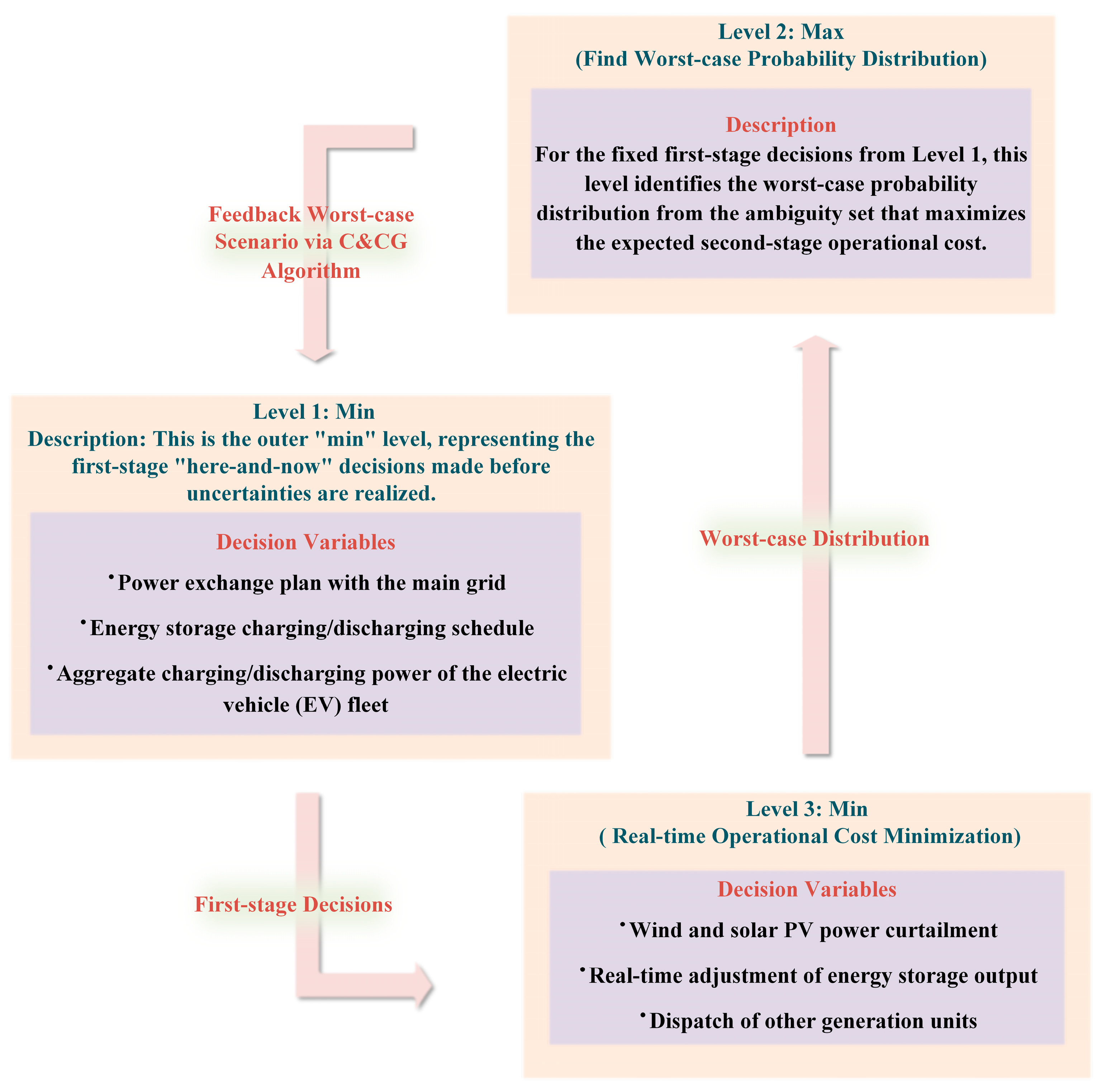
As shown in Figure 2, this paper constructs a two-stage distributionally robust optimization (DRO) scheduling framework for a typical microgrid system to address the inherent randomness and volatility of renewable energy sources. It is crucial to clarify the model’s architecture: the “two-stage” defines the temporal sequence of decisions, while the “three-level min-max-min” structure describes the mathematical approach to solving the optimization problem under uncertainty.

• Temporal Decision Stages

The model operates across two temporal stages. The first stage (Day-ahead Scheduling) makes “here-and-now” decisions before uncertainties are realized, determining the power exchange schedule, energy storage plans, and aggregate EV fleet power. The second stage (Real-time Dispatch) makes “wait-and-see” adjustments after uncertainties are known, dispatching fast-regulating resources to correct deviations from the day-ahead plan.

2.

Optimization Levels

The core optimization problem is structured in three levels. The first level (Min) determines the optimal day-ahead decisions. The second level (Max) identifies the worst-case probability distribution from the ambiguity set. The third level (Min) then optimizes the real-time decisions under that worst-case distribution.

The decision variables for each stage are explicitly defined in

Table 1. Definition of decision variables in the two-stage DRO model.

Decision Stage	Category	Decision Variables	Symbol
Stage1 (Day-ahead)	Microgrid Trading	Power purchased from the main grid	$P_t^{\mathrm{Buy}}$
		Power is sold to the main grid.	$P_t^{S\mathrm{ell}}$
	Energy Storage	Charging power	$P_t^{\mathrm{e}\_\mathrm{ch}}$
		Discharging power	$P_t^{\mathrm{e}\_\mathrm{dis}}$
	Electric Vehicle Fleet	Aggregate charging power	$P_{u,t}^{\mathrm{ev}}$
		Aggregate discharging power	$P_{u,t}^{\mathrm{ev}}$
Stage2 (Real-time)	Unit Dispatch & Balancing	Realized PV power curtailment	$P_{s,t}^{r,N}$
		Realized wind power curtailment	$P_{s,t}^{r,W}$
		Actual charging power of energy storage (adjustment)	$P_{s,t}^{\mathrm{e}\_\mathrm{ch}}$
		Actual discharging power of energy storage (adjustment)	$P_{s,t}^{\mathrm{e}\_\mathrm{dis}}$

.

The overall objective of this framework is to minimize the total expected operating cost, which comprises the power exchange cost with the primary grid, the operating cost of electric vehicles, and the penalty cost for wind and solar curtailment.

The advantage of this DRO framework is that it neither relies on the difficult-to-obtain accurate probability distribution (as stochastic programming does) nor suffers from the excessive conservatism of traditional robust optimization. By seeking the optimal decision under the worst-case distribution within an ambiguity set, it produces a scheduling strategy that is both robust and economical.

In the initial phase, decision variables include the power consumption and sale plan of the distribution network, the energy storage charging and discharging schedule, and Electric vehicle charging and discharging power; in the second stage, the decision variables are the outputs of each unit. Upon realization of uncertainties, a scheduling plan for the Microgrid is developed. In the model’s outer layer, the min function serves to achieve the overall objective through comprehensive optimization. At the middle layer of the model, the max function is used to maximize the expected second-stage cost within the given probability distribution ambiguity set, thereby determining the worst-case probability distribution. At the inner layer of the model, the min occasion aims to diminish the expected second-stage cost.

The optimization objective proposed in this paper can be conveyed as follows:

$$\begin{array}{l}\min F\\ =\underset{x}{\min }{F}_{\mathrm{ev}}+\underset{{\sigma }^s\in \Omega }{\max }\underset{y}{\min }{\displaystyle \sum _{\mathrm{s}=1}^{\mathrm{N}}{\sigma }^{\mathrm{s}}(F_{\mathrm{grid}}^{\mathrm{s}}+F_{\mathrm{cur}}^{\mathrm{s}})}\end{array}$$

(1)

In the equation, x and y represent the decision variables of the first and second stages, respectively, σ^s characterizing the probability of occurrence of the s-th scenario, Ω denotes the probability distribution ambiguity set, and N is the total number of scenarios considered.

(1)

First stage: the charging and discharging costs of electric vehicles.

$$F_{\mathrm{ev}}={\displaystyle \sum _{t=1}^T{\displaystyle \sum _{u=1}^U{\omega }_{\mathrm{ev},t}{P}_{u,t}^{\mathrm{ev}}}}$$

(2)

In the equation: ω_ev,t Charging and discharging cost of the electric vehicle at time t.

(2)

Second Stage: Collaboration cost between the Microgrid and the distribution network, as well as the costs of wind curtailment and photovoltaic curtailment.

$$F_{\mathrm{grid}}^{\mathrm{s}}=\sum _{s=1}^S\sum _{t=1}^T\left({\omega }_{\mathrm{M},t}^{\mathrm{Buy}}{P}_{s,t}^{\mathrm{Buy}}-{\omega }_{\mathrm{M},t}^{\mathrm{Sell}}{P}_{s,t}^{\mathrm{Sell}}\right)$$

(3)

$$F_{\mathrm{cur}}^{\mathrm{s}}=\sum _{s=1}^S\sum _{t=1}^T\omega \left(P_{s,t}^{r,N}+P_{s,t}^{r,\mathrm{W}}\right)$$

(4)

In the equation: ${\omega }_{\mathrm{M},t}^{\mathrm{Buy}}$, ${\omega }_{\mathrm{M},t}^{\mathrm{Sell}}$ The electricity acquisition and sale prices at period t, respectively; $\omega$ Unit economic penalty coefficient for wind curtailment and photovoltaic curtailment.

2.2. Electric Energy Storage Model

Electric energy storage devices can store electricity when wind turbines and photovoltaic power production exceed load demand and release it during peak load periods. The electric energy storage model is expressed as:

$$\begin{array}{l}{E}_{s,t}^{\mathrm{e}}=E_{s,t-1}^{\mathrm{e}}+\\ \left(P_{s,t}^{\mathrm{e}\_\mathrm{ch}}{\mu }_{e_{-}ch}-P_{s,t}^{\mathrm{e}\_\mathrm{dis}}/{\mu }_{e_{-}dis}\right)\Delta t\end{array}$$

(5)

In the equation: $E_{s,t}^{\mathrm{e}}$ State of charge of the energy storage battery at retro t under scenario s; $P_{s,t}^{\mathrm{e}\_\mathrm{ch}}$, $P_{s,t}^{\mathrm{e}\_\mathrm{dis}}$ denotes the charging and discharging power during the s th scenario and tth time interval, ${\mu }_{\mathrm{e}\_\mathrm{ch}}$, ${\mu }_{\mathrm{e}\_\mathrm{dis}}$ represents the charging and discharging efficiency, and Δt denotes the time interval.

2.3. Demand Response Model

Demand response enhances grid flexibility by actively managing load profiles. This paper models two primary types of flexible loads: shiftable loads and interruptible loads, each with distinct physical characteristics. Shiftable loads, such as washing machines or electric vehicle charging (when not acting as a power source), represent tasks whose operation can be delayed or advanced in time without affecting the service provided to the user. The key is to shift energy consumption away from expensive peak periods to lower-cost off-peak times. In contrast, interruptible loads, typified by air conditioners, have inherent thermal inertia. This means they can be temporarily turned off or reduced without causing an immediate, uncomfortable change in the indoor environment. The building itself acts as a thermal energy storage buffer, allowing the load to be modulated for grid support while maintaining temperature within a comfortable band. The following mathematical models formalize these physical principles into operational constraints for the microgrid scheduling problem.

2.3.1. Shiftable Load Model

Shiftable load is a demand-side management strategy that motivates users to proactively adjust their load distribution across time periods by modifying electricity price structures or applying economic incentives. Its mathematical expression is: [15]

$$D_{s,t}^{\mathrm{DR}}-D_{s,t}+D_{s,t}^{\mathrm{DR},1}-D_{s,t}^{\mathrm{DR},2}=0$$

(6)

$D_{s,t}$ and $D_{s,t}^{\mathrm{DR}}$, respectively, denote the actual microgrid load levels before and after demand response in the tth interval of the sth scenario, and represents the demand response reduction ratio.

2.3.2. Interruptible Load Model

An important representative is the air conditioner; the model can be expressed as:

$$\begin{array}{l}{\theta }_{s,t+1}^{\mathrm{in}}={\mathrm{e}}^{{\displaystyle \frac{-\Delta t}{RC}}}{\theta }_{s,t}^{\mathrm{in}}+{\displaystyle \frac{\Delta tR}{C}}(1-{\mathrm{e}}^{{\displaystyle \frac{-\Delta t}{RC}}})Q_{s,t}{B}_{s,t}^Q+\\ ({\mathrm{e}}^{{\displaystyle \frac{-\Delta t}{RC}}}-1){\theta }_{s,t}^{\mathrm{out}}\end{array}$$

(7)

In the formula: ${\theta }_{s,t}^{\mathrm{in}}$ Indoor temperature at time period t in scenario s; ${\theta }_{s,t+1}^{\mathrm{in}}$ Indoor temperature at time period t + 1 in scenario s. ${\theta }_{s,t}^{\mathrm{out}}$ Outdoor temperature; R is the thermal insulation coefficient; C is the building’s thermal capacity; Δ t is the time interval; $Q_{s,t}$ Air conditioner power at time period t in scenario s; $B_{s,t}^Q$ Binary variable indicating the air conditioner activation state.

2.3.3. Electric Vehicle Model

Electric vehicle charging and discharging are affected by various factors, including arrival time, departure time, and expected state of charge. As distributed generation, electric vehicles can absorb load through charging and supply power to the Microgrid through discharging, thereby achieving peak shaving and valley stuffing. The cluster electric vehicle model proposed in this paper accurately captures the influence of coordinated charging of multiple electric vehicles on the Microgrid.

The cluster electric vehicle model is defined as:

State of Charge of Electric Vehicles $E_{u,t}^{\mathrm{ev}}$ Influenced by charging and discharging power, the variation formula is

$$\begin{array}{l}{E}_{u,t}^{\mathrm{ev}}=E_{u,t-1}^{\mathrm{ev}}+{\mu }^{\mathrm{ev}\_\mathrm{ch}}{P}_{u,t}^{\mathrm{ev}\_\mathrm{ch}}\Delta t-{\displaystyle \frac{P_{u,t}^{\mathrm{ev}\_\mathrm{dis}}\Delta t}{{\mu }^{\mathrm{ev}\_\mathrm{dis}}}},\\ t\in T_u^{\mathrm{ev}}\end{array}$$

(8)

The modeling of EV uncertainty and its integration has been studied in network reconfiguration considering DG and EVs [16], and the temporal correlation of wind power uncertainty has been modeled using polyhedral sets [17]. Furthermore, collaborative scheduling of active distribution networks and multiple microgrids considering renewable uncertainties has also been investigated [18].

2.4. Constraints

(1)

Power interaction balance constraint of the Microgrid

$$\begin{array}{l}{P}_{s,t}^{\mathrm{Buy}}+P_{s,t}^{\mathrm{S}}+P_{s,t}^{\mathrm{W}}+P_{s,t}^{\mathrm{d}}=D_{s,t}^{\mathrm{DR}}+P_{s,t}^{\mathrm{Sell}}+\\ P_{s,t}^{\mathrm{c}}+N_{\mathrm{Ro}}{Q}_{s,t}{B}_{s,t}^Q\end{array}$$

(9)

$$P_{s,t}^{\mathrm{MG}}=P_{s,t}^{\mathrm{Sell}}-P_{s,t}^{\mathrm{Buy}}$$

(10)

In the equation: $P_{s,t}^{\mathrm{S}}$ and $P_{s,t}^{\mathrm{W}}$ For the microgrid generation, $P_{s,t}^{\mathrm{d}}$ For load demand, $P_{s,t}^{\mathrm{Buy}}$, $P_{s,t}^{\mathrm{Sell}}$, respectively, are the purchased electricity amount and the sold electricity amount. $N_{\mathrm{Ro}}$ Number of typical rooms. The equivalent power of electricity procured and traded by the Microgrid during the time period t.

(2)

Energy Storage Constraints

$$E_{\min }^e\le E_{s,t}^{\mathrm{e}}\le E_{\max }^{\mathrm{e}}$$

(11)

$$E_{s,t=24}^{\mathrm{e}}=E_{s,t=0}^{\mathrm{e}}$$

(12)

$$0\le P_{s,t}^{\mathrm{e}\_\mathrm{ch}}\le B_{s,t}^{\mathrm{e}\_\mathrm{ch}}{P}_{\max }^{\mathrm{e}\_\mathrm{ch}}$$

(13)

$$0\le P_{s,t}^{\mathrm{e}\_\mathrm{dis}}\le B_{s,t}^{\mathrm{e}\_\mathrm{dis}}{P}_{\max }^{\mathrm{e}\_\mathrm{dis}}$$

(14)

$$B_{s,t}^{\mathrm{e}\_\mathrm{ch}}+B_{s,t}^{\mathrm{e}\_\mathrm{dis}}\le 1$$

(15)

In the equation: $P_{s,t}^{\mathrm{e}\_\mathrm{ch}}$, $P_{s,t}^{\mathrm{e}\_\mathrm{dis}}$ Denotes the charging and discharging power during the sth scenario and tth time interval, $P_{\max }^{\mathrm{e}\_\mathrm{ch}}$, $P_{\max }^{\mathrm{e}\_\mathrm{dis}}$ Maximum charging and discharging power; $B_{s,t}^{\mathrm{e}\_\mathrm{ch}}$, $B_{s,t}^{\mathrm{e}\_\mathrm{dis}}$ Binary variable for charging and discharging; $E_{s,t=0}^{\mathrm{e}}$ Initial energy storage capacity; Δt denotes the time interval.

(3)

Demand Response Coefficient Constraints

$$0\le {\alpha }_{s,t}\le {\alpha }_{s,t}^{\max }$$

(16)

$${\mathrm{P}}_{s,t}^{\mathrm{Inc}}\ge 0,D_{s,t}^{\mathrm{DR},1}\ge 0,D_{s,t}^{\mathrm{DR},2}\ge 0$$

(17)

$${\theta }_{\min }^{\mathrm{in}}\le {\theta }_{s,t}^{\mathrm{in}}\le {\theta }_{\max }^{\mathrm{in}}$$

(18)

In the equation, ${\alpha }_{s,t}^{\max }$ the Maximum achievable value of the demand response coefficient, $D_{s,t}^{\mathrm{DR},1}$ and $D_{s,t}^{\mathrm{DR},2}$ two introduced auxiliary variables. ${\theta }_{\min }^{\mathrm{in}}$ And ${\theta }_{\max }^{\mathrm{in}}$ the Minimum and maximum indoor temperature.

(4)

Electric Vehicle Related Constraints

$$0⩽P_{u,t}^{\mathrm{ev}\_\mathrm{ch}}⩽P_{\max ,u}^{\mathrm{ev}\_\mathrm{ch}},\hspace{1em}t\in T_u^{\mathrm{ev}}$$

(19)

$$0⩽P_{u,t}^{\mathrm{ev}\_\mathrm{dis}}⩽P_{\max ,u}^{\mathrm{ev}\_\mathrm{dis}},\hspace{1em}t\in T_u^{\mathrm{ev}}$$

(20)

$$C_{u,t}=\left\{\begin{array}{c}0,\mathit{\forall }t\notin \left[T_u^{\mathrm{arr}},T_u^{\mathrm{lea}}\right]\\ 1,\mathit{\forall }t\in \left[T_u^{\mathrm{arr}},T_u^{\mathrm{lea}}\right]\end{array}\right.$$

(21)

$$E_u^{\mathrm{ev}\_\min }⩽E_{u,t}^{\mathrm{ev}}⩽E_u^{\mathrm{ev}\_\min },t\in T_u^{\mathrm{ev}}$$

(22)

In the equation: $P_{u,t}^{\mathrm{ev}\_\mathrm{ch}}$ and $P_{u,t}^{\mathrm{ev}\_\mathrm{dis}}$ Charging power and discharging power of electric vehicle for user u at time t, respectively; $P_{\max ,u}^{\mathrm{ev}\_\mathrm{ch}}$ and $P_{\max ,u}^{\mathrm{ev}\_\mathrm{dis}}$ Maximum charging and discharging power values, respectively. $C_{u,t}$ Availability status of the electric vehicle at time t, taking values 0 or 1; $T_u^{\mathrm{arr}}$ and $T_u^{\mathrm{lea}}$ respectively, the arrival time and departure time; Δt represents the time interval.

(5)

Microgrid electricity purchase and sale constraints

$$0⩽P_{s,t}^{\mathrm{Buy}}⩽B_{s,t}^{\mathrm{Buy}}{P}_{\max }^{\mathrm{Buy}}$$

(23)

$$0⩽P_{s,t}^{\mathrm{Sell}}⩽B_{s,t}^{\mathrm{Sell}}{P}_{\max }^{\mathrm{Sell}}$$

(24)

In the equation: $P_{s,t}^{\mathrm{Buy}}$, $P_{s,t}^{\mathrm{Sell}}$ Respectively, the maximum values for electricity purchase and sale $B_{x,t}^{\mathrm{Buy}}$, $B_{x,t}^{\mathrm{Sell}}$ represent the Microgrid’s electricity purchase and sale status with the distribution network.

2.5. Per-Unit System Normalization

To facilitate numerical stability and generalization of the model, all power (kW) and energy (kWh) variables in this paper are expressed in the per-unit (p.u.) system. The base power value $S_{\mathrm{b}}$ is chosen as 500 kW. Consequently, the base energy value $E_{\mathrm{b}}$ is 500 kWh for a 1-h time interval. All subsequent power and energy-related variables and parameters are normalized using these base values.

3. Construction of Ambiguity Sets for Wind-Photovoltaic Generation Output and Explanation of the Distributionally Robust Optimization Model

This section is dedicated to constructing the two-stage distributionally robust optimization (DRO) model and developing the corresponding solution algorithm. The proposed methodology is designed to achieve robust and economical scheduling for the Microgrid under renewable uncertainty. Firstly, the basic framework of the model, including its “min-max-min” structure and two-stage decision-making sequence, is elaborated in Section 3.1. Furthermore, the precise mathematical formulations for both the first and second-stage problems are presented in Section 3.2, defining the objective functions and constraints.

3.1. Construction of Ambiguity Sets for Wind-Photovoltaic Generation Output Based on KL Divergence

3.1.1. Motivation for KL Divergence and Comparison with Wasserstein Metric

The Kullback–Leibler (KL) divergence is selected to construct the ambiguity set in this work, primarily due to its computational tractability and practical applicability in engineering settings.

The key motivation for adopting the KL divergence lies in its ability to quantitatively measure the information loss when a reference distribution $P_0$ is used to approximate the true distribution P. This property makes it particularly suitable for characterizing distributional uncertainty in contexts where only limited historical data are available.

A further advantage of the KL divergence emerges when compared to alternative methods such as the Wasserstein metric. While Wasserstein-based ambiguity sets often lead to computationally intensive, non-convex optimization problems—especially in multi-level frameworks like the one presented here—the KL divergence generally preserves convexity. This characteristic is crucial for the efficient solution of our three-level min–max–min problem using the Column-and-Constraint Generation (C&CG) algorithm. Moreover, the KL divergence requires only a reference distribution for its construction, eliminating the need to estimate higher-order moments, which are often difficult to obtain reliably. This feature significantly enhances its practicality in real-world microgrid scheduling applications, where data may be scarce or uncertain.

3.1.2. Reference Distribution of Wind-Photovoltaic Generation $P_0$

To construct ambiguity sets based on probability distributions, it is first necessary to determine the reference distribution of the uncertain parameters. This paper adopts the Latin Hypercube method combined with the Synchronous Backward Scenario Reduction method to generate reference distributions of wind power and photovoltaic output [9]. The synchronous rearward scenario discount process can be used to select representative scenarios and specify their probabilities. Specifically, the prospect of each wind power and photovoltaic scenario can be calculated by the following formula

$$P_k^0={\displaystyle \frac{M_k}{M}}$$

(25)

In the formula, $M$ denotes the set of historical output samples, $M_k$ and denotes the number of original scenarios contained within the reduced typical scenarios.

The reference distribution can be formally expressed as

$$P_0=\{{\displaystyle \frac{M_1}{M}},{\displaystyle \frac{M_2}{M}},\dots ,{\displaystyle \frac{M_k}{M}}\}$$

(26)

3.1.3. Establishing the Ambiguity Set $\zeta$

This paper introduces the Kullback–Leibler (KL) divergence to construct the uncertainty ambiguity set for wind-solar outputs. KL divergence, as an important metric in information theory, can precisely quantify the disparity between two probability distributions, thereby characterizing the similarity between the actual distribution of wind-solar outputs and the reference distribution. The formula for calculating the KL divergence is

$$D_{\mathrm{KL}}(P\parallel P_0)=\sum _{n=1}^N{p}_{n}In{\displaystyle \frac{p_n}{p_n^0}}$$

(27)

In the formula, N represents the dimension of the sample space, $p_n$ and represents the value of the probability distribution function P at the sample point n, $p_n^0$ as the reference distribution function $P_0$ at the same sample point n. Accordingly, the mathematical expression of the ambiguity set can be

$$\zeta =\{P\mid D_{\mathrm{KL}}(P\parallel P_0)⩽d_{\mathrm{KL}}\}$$

(28)

In the formula, $P_0$ represents the reference distribution defined in Equation (32). $d_{\mathrm{KL}}$ Represents the set distance, indicating the reference distribution function $P_0$ and the similarity threshold of the probability distribution function P. The greater this value, the stronger the robustness of the model, and the more conservative the optimization strategy tends to be.

3.1.4. Determination of Set Distance $\rho$

The set distance parameter $\rho$ is the key to controlling the conservativeness of the distributionally robust optimization model. Decision-makers generally determine its value based on their actual risk preference. Physically, $\rho$ represents a risk-aversion parameter. It defines the maximum “tolerance” allowed for the true distribution to deviate from the reference distribution. A larger $\rho$ value indicates a higher degree of risk aversion, meaning the decision-maker considers a wider range of possible distributions (a larger ambiguity set D), leading to a more conservative and robust scheduling strategy.

The value $\rho$ should be set in relation to the volume and quality of available historical data. Considering that the larger the amount of historical data, the closer the reference distribution is to the true probability distribution, at this time, $\rho$ a smaller value can be set; conversely, if the data is insufficient, it should be appropriately increased. $\rho$ The value. Specifically, $\rho$ the value can be determined by the following formula:

$$\rho ={\displaystyle \frac{1}{2N}}{\chi }_{R-1,{\alpha }^{\ast }}^2$$

(29)

In the formula, N is the number of days covered by the historical data; ${\chi }_{R-1,{\alpha }^{\ast }}^2$ is the upper quantile of the chi-square distribution D, ensuring that the true distribution is contained within set D with a probability no less than α^∗.

3.2. Solution Method for the Distributionally Robust Optimization Model

After constructing the probability ambiguity set based on KL divergence, the model adopts a two-stage progressive optimization solution strategy: The first stage defines whether the Microgrid desires to purchase or sell electricity with the upstream grid, the charging and discharging plans of the energy storage devices, and the charging and discharging power of the electric vehicle fleet; In stage 2, a corresponding scheduling strategy is formulated after the realization of the preceding uncertainty. The proposed Microgrid distributionally robust optimization model can be simplified into the following form [19,20,21]:

$$\left\{\begin{array}{l}\underset{L,X}{\min }{\mathit{C}}^T\mathit{X}+\underset{\delta \in D}{\max }{\displaystyle \sum _{s=1}^S}{\delta }_s\underset{Y_s,L_s^u}{\min }{\mathit{D}}^{\mathrm{T}}{\mathit{Y}}_s\\ \mathrm{s}.\mathrm{t}.\left\{\begin{array}{c}\mathit{A}\mathit{X}+\mathit{B}{\mathit{Y}}_s+\mathit{C}{\mathit{L}}_s^u⩽\mathit{h}\\ \mathit{L}\in \{0,1\}& \\ {\mathit{L}}_s^u\in \{0,1\}\end{array}\right.\end{array}\right.$$

(30)

In the equation: $\mathit{X}$ are the decision variables of stage 1, $\mathit{L}$, ${\mathit{L}}_s^u$ are the 0–1 variables in the stage 1 and stage 2 optimization models, respectively; ${\mathit{Y}}_s$ are the continuous variables in the stage 2 optimization problem; ${\delta }_s$ are the probabilities of the corresponding scenario s; S is the total number of scenarios; ${\mathit{D}}^T$, A, B, C, h are all constant coefficient matrices.

The specific composition of the above optimization variables can be further expressed as:

$$\left\{\begin{array}{c}\begin{array}{l}\mathit{X}={\left[P_{u,t}^{\mathrm{ev}\_\mathrm{ch}},P_{u,t}^{\mathrm{ev}\_\mathrm{dis}},E_{u,t}^{\mathrm{ev}}\right]}^{\mathrm{T}}\\ \mathit{L}={\left[B_{s,t}^c,B_{s,t}^{\mathrm{d}},B_{s,t}^{\mathrm{Buy}},B_{s,t}^{\mathrm{Sell}}\right]}^{\mathrm{T}}\end{array}\\ {\mathit{Y}}_s={\left[\begin{array}{c}{D}_{s,t}^{\mathrm{DR}},{\mathrm{DR}}_{s,t},{\mathrm{P}}_{s,t}^{\mathrm{Inc}},{\theta }_{s,t}^{\mathrm{in}},P_{s,t}^{e\_ch},P_{s,t}^{e\_dis},\\ E_{s,t}^e,P_{s,t}^{\mathrm{Buy}},P_{s,t}^{\mathrm{Sell}},D_{s,t}^{\mathrm{DR},1},D_{s,t}^{\mathrm{DR},2}\end{array}\right]}^{\mathrm{T}}\\ {\mathit{L}}_s^u={\left[B_{s,t}^Q\right]}^{\mathrm{T}}\end{array}\right.$$

(31)

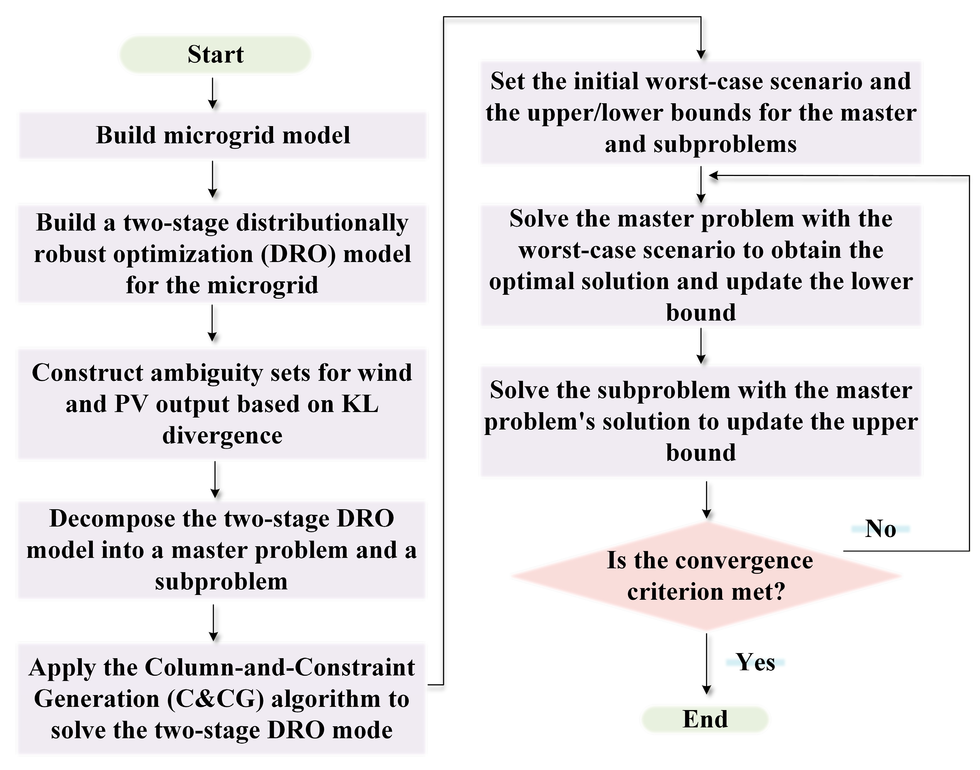
To unravel the above two-stage min–max–min distributionally robust optimization difficulty, this paper adopts a solution strategy based on the Column-and-Constraint Generation (C&CG) algorithm. This method first decouples the model into a master setback and a subproblem, and afterward iteratively approaches the global optimum solution, achieving convergence.

3.2.1. Master Problem

During the solution process of the master problem, whenever the most critical risk scenario is identified in the inner loop, it is fed back to the master problem, introducing a set of new variables, which leads to re-solving the master problem. The mathematical model is described as follows:

$$\begin{array}{c}\underset{\mathit{X},\mathit{L},\eta ,{\mathit{Y}}_s^w,{\mathit{L}}_s^{u,w},w=1,2,\dots ,V}{\min }\eta \\ \mathrm{s}.\mathrm{t}.\left\{\begin{array}{c}{\displaystyle \sum _{s=1}^S}{\delta }_s^{\ast ,w}{\mathit{D}}^{\mathrm{T}}{\mathit{Y}}_s^w\le \eta ,\\ \mathit{A}\mathit{X}+\mathit{B}{\mathit{L}}_s^{u,w}+\mathit{B}{\mathit{Y}}_s^w\le \mathit{h},\\ \eta \ge 0,\\ \mathit{L}\in \{0,1\},\\ {\mathit{L}}_s^{u,w}\in \{0,1\},\\ \forall 1\le w\le V.\end{array}\right.\end{array}$$

(32)

In the equation, $\eta$ as an intermediate variable, it represents the estimation value for the Subproblem; V $w$ denotes the total number of outer loop iterations and the current iteration count; ${\delta }_s^{\ast ,w}$ and is the $w$ distribution probability of the most critical scenario at the iteration. Thus, the master problem provides a lower bound for the innovative problem. ${\mathrm{m}}_{\mathrm{out}}$, while the Subproblem obtains the upper bound of the innovative difficulty ${\mathrm{M}}_{\mathrm{out}}$. When the superior and lower bounds satisfy a certain error tolerance, i.e., when the gap between the upper and lower bounds meets the preset error threshold, the model can be considered united, i.e.,

$$\left|{\mathrm{M}}_{\mathrm{out}}-{\mathrm{m}}_{\mathrm{out}}\right|⩽E_{\mathrm{out}}$$

(33)

In the formula, $E_{\mathrm{out}}$ is a very small positive number.

3.2.2. Subproblem

The inner subproblem points to classify the worst-case scenario distribution probability and convey this information back to the master problem. Its model is defined as

$$\left\{\begin{array}{c}\underset{\delta \in D}{\max }{\displaystyle \sum _{s=1}^S}{\delta }_s\underset{{\mathit{Y}}_s,{\mathit{L}}_s^u}{\min }{\mathit{D}}^{\mathrm{T}}{\mathit{Y}}_s\\ \mathrm{s}.\mathrm{t}.\left\{\begin{array}{ccc}\mathit{A}{\mathit{X}}^{\ast }+\mathit{B}{\mathit{Y}}_s+\mathit{C}{\mathit{L}}_s^u⩽\mathit{h}& & \\ {\mathit{L}}_s^u\in \{0,1\}& & \end{array}\right.\end{array}\right.$$

(34)

Here, ${\mathit{X}}^{\ast }$ represents the first-stage conclusion values attained from the master problem, which are treated as parameter constants in this Subproblem. At this stage, this Subproblem is a bilevel optimization problem with integer variables, and the nonlinear terms in the objective function make direct application of KKT conditions or strong duality theory challenging however, since the lower-level objective function is a fixed scalar and does not affect the feasibility domain of the constraints, a stepwise decoupling strategy can be adopted to decompose this Subproblem into two independent steps, thereby simplifying the computational process.

Step 1: Solve the lower-level mixed-integer linear programming models, which can be formulated as

$$\left\{\begin{array}{c}{h}_s^{\ast }=\underset{Y_s,L_s^u}{\min }{\mathit{D}}^{\mathrm{T}}{\mathit{Y}}_s\\ \mathrm{s}.\mathrm{t}.\left\{\begin{array}{cc}\mathit{A}{\mathit{X}}^{\ast }+\mathit{B}{\mathit{Y}}_s+\mathit{C}{\mathit{L}}_s^u⩽\mathit{h}& \\ {\mathit{L}}_s^u\in \{0,1\},& \\ s=1,2,\dots ,S& \end{array}\right.\end{array}\right.$$

(35)

Step 2: Substitute the optimal solution obtained in the lower level from Step 1 into the upper-level problem, i.e.,

$$\underset{\delta \in D}{\max }\sum _{s=1}^S{\delta }_s{h}_s^{\ast }$$

(36)

At this stage, based on the above calculations, the upper bound M of the original problem can be resolved. Notably, although the upper-level model exhibits a nonlinear structure, the convexity of the KL divergence ambiguity set ensures that the overall problem maintains convex optimization characteristics, thereby enabling the determination of a global optimum. Through this decomposition method, the subproblem solution can be effectively transmitted to the master problem for iterative optimization.

3.2.3. Solution Method Based on the C&CG Algorithm

The Column-and-Constraint Generation (C&CG) algorithm decomposes the problem into a Master Problem (MP) and a Subproblem (SP), which are solved iteratively:

• MP minimizes costs given a set of critical scenarios;
• SP finds the worst-case distribution for fixed first-stage decisions;
• Iteration continues until bounds converge.

The iterative procedure is detailed as follows:

Step 1: Initialize iteration counter $w=1$, upper bound ${\mathrm{M}}_{\mathrm{out}}=+\infty$, and lower bound ${\mathrm{m}}_{\mathrm{out}}=-\infty$ tolerance $E_{\mathrm{out}}$.

Step 2: Obtain the first-stage decision ${\mathit{X}}^{\ast }$. Update ${\mathrm{m}}_{\mathrm{out}}=\max \{{\mathrm{m}}_{\mathrm{out}},{\eta }^{\ast }\}$

Step 3: Fix ${\mathit{X}}^{\ast }$ and find the worst-case distribution. Update ${\mathrm{M}}_{\mathrm{out}}=\min \{{\mathrm{M}}_{\mathrm{out}},{\eta }^{\ast }\}$

Step 4: If $\left|{\mathrm{M}}_{\mathrm{out}}-{\mathrm{m}}_{\mathrm{out}}\right|⩽E_{\mathrm{out}}$, stop the iteration and output the results;

Step 5: Add optimality cut from SP to MP. Set $w=w+1$ goes to Step 2.

This iterative process continues until the gap between the upper and lower bounds meets the convergence criterion, ensuring a globally optimal solution is found.

As shown in Figure 3, the solution methodology is based on the Column-and-Constraint Generation (C&CG) algorithm, which operates through a cycle of decomposition and iterative refinement. The original complex optimization model is first decomposed into a Master Problem, which determines the day-ahead scheduling decisions, and a Subproblem that accounts for real-time uncertainties in wind and photovoltaic output. The algorithm proceeds iteratively: the Master Problem generates first-stage decisions, which are then passed to the Subproblem to identify the most adverse probability distribution of renewable generation under those decisions. The Subproblem’s outcome is subsequently fed back to the Master Problem, enabling it to adjust and improve the decisions. This cycle continues until the gap between the lower bound provided by the Master Problem and the upper bound provided by the Subproblem narrows sufficiently, indicating convergence and resulting in a scheduling plan that effectively balances economic efficiency with operational robustness.

4. Case Study Analysis

Following the mathematical formulation and solution algorithm presented in Section 3, this section proceeds to the numerical validation of the proposed DRO framework. The objective is to assess its practical performance using a realistic microgrid test case. The structure of this section is organized as follows: it begins with a description of the case study setup, including the system parameters and defined scenarios. It then presents and discusses the simulation results, focusing on scheduling outcomes and cost analysis. The section concludes with a comparative study to quantify the benefits of the proposed model against traditional scheduling methods.

4.1. Basic Microgrid Data

The paper selects a microgrid in Central China (structure shown in Figure 1) as the test case to validate the efficacy of the projected distributionally robust optimization model and algorithm. The microgrid parameters and time-of-use electricity prices are detailed in

Table 2. Microgrid Parameters.

Parameter	Value	Parameter	Value
${\alpha }_{s,t}^{\max }$	0.3	${\mu }_{\mathrm{e}\_\mathrm{ch}}$, ${\mu }_{\mathrm{e}\_\mathrm{dis}}$	0.95, 0.90
${\Delta }_{\max }^{\mathrm{DR}}$, ${\Delta }_{\min }^{\mathrm{DR}}$	0.3, 0.3	$E_{\max }^{\mathrm{e}}$, $E_{\min }^{\mathrm{e}}$	100, 0
$R$/°C	18	$E_{s,t=0}^{\mathrm{e}}$ (p.u.)	0.2
$C$/(kW·h·(°C)−1)	0.525	$P_{s,t}^{\mathrm{Buy}}$, $P_{s,t}^{\mathrm{Sell}}$/kW	500, 500
${\theta }_{s,t}^{\mathrm{in}}$, ${\theta }_{s,t}^{\mathrm{out}}$/°C	26.24	$T_{\mathrm{set}}$/°C	25
$\rho$	0.01	$N_{\mathrm{Ro}}$	6
$P_{\max }^{\mathrm{e}\_\mathrm{ch}}$, $P_{\min }^{\mathrm{e}\_\mathrm{ch}}$/kW	20, 20	$P_{\max ,u}^{\mathrm{ev}\_\mathrm{ch}}$, $P_{\min ,u}^{\mathrm{ev}\_\mathrm{ch}}$	0.98, 0.98

and

Table 3. Electricity Purchase and Sale Prices.

Time Period	Electricity Purchase Price/(yuan/kWh)	Electricity Sale Price/(yuan/kWh)
00:00–07:00	0.43405	0.33405
08:00–22:00	0.78405	0.68405
12:00–15:00	0.63405	0.53405
16:00–18:00	0.78405	0.68405
19:00–22:00	0.88405	0.78405
23:00–24:00	0.43405	0.33405

, respectively. Furthermore, to account for the uncertainties of wind power and photovoltaics, this paper employs forecast data of wind power and photovoltaics and applies the Latin hypercube sampling method to generate 1000 scenarios. Subsequently, the synchronous retrograde substitution discount way is used to screen five normal discrete scenarios and obtain the initial probability values for these five typical scenarios. This study evaluates the proposed model under five typical scenarios:

(1)

Base Case with normal renewable generation and load;

(2)

High Renewable Generation with high PV/wind output;

(3)

Low Renewable Generation with scarce renewable availability;

(4)

High Load Demand representing a peak load condition;

(5)

EV Charging Peak with concentrated electric vehicle charging loads.

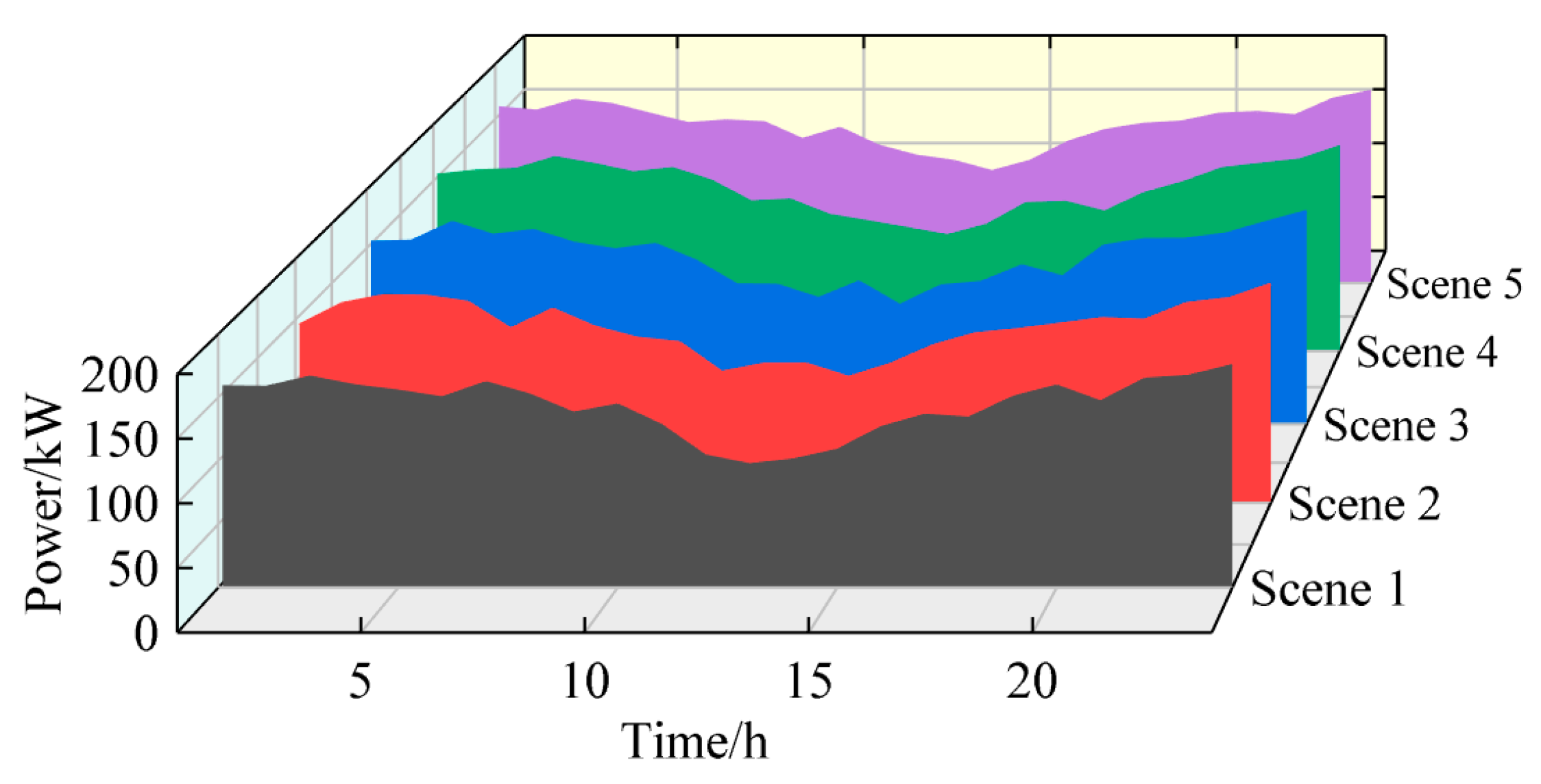
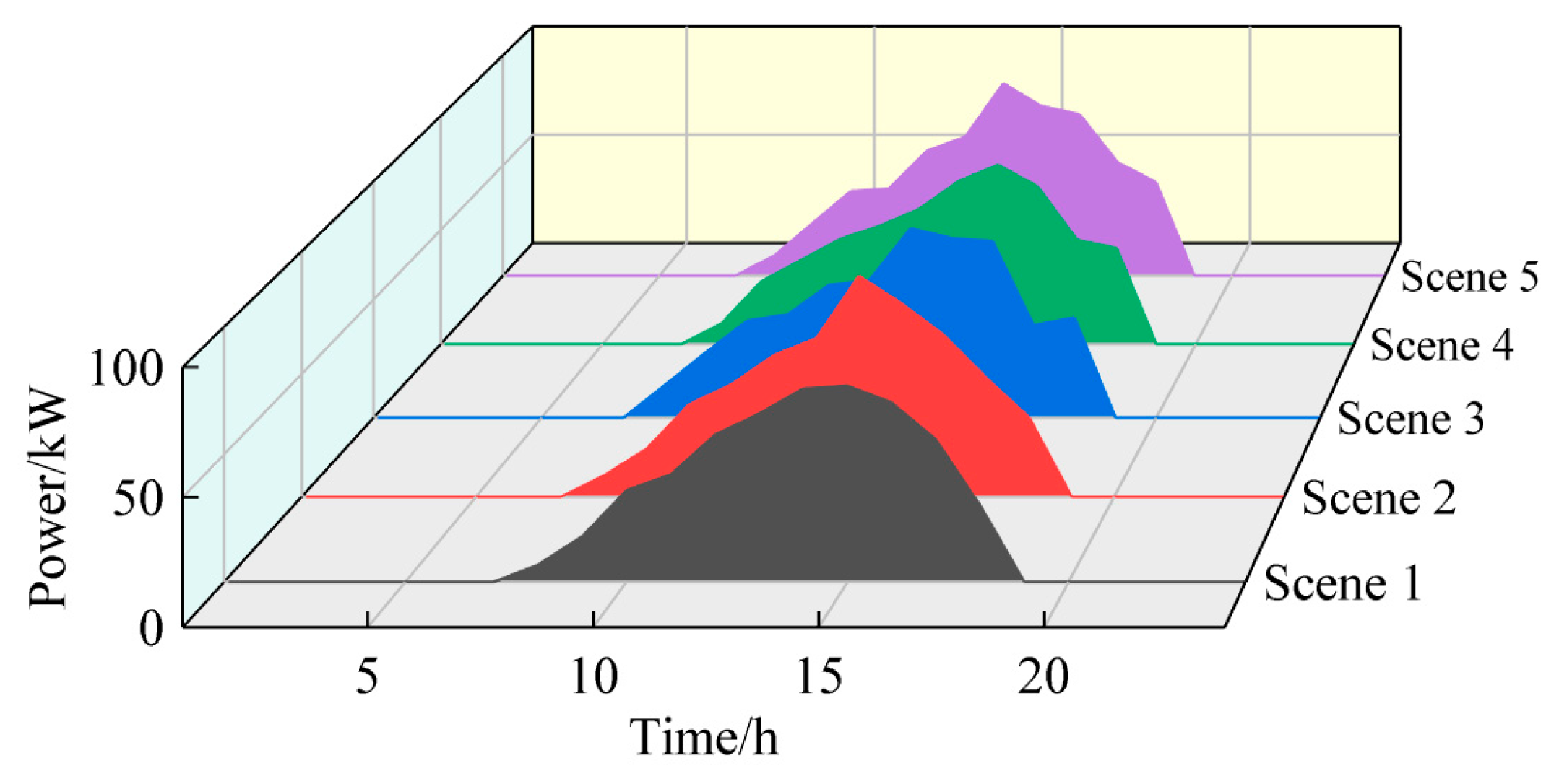
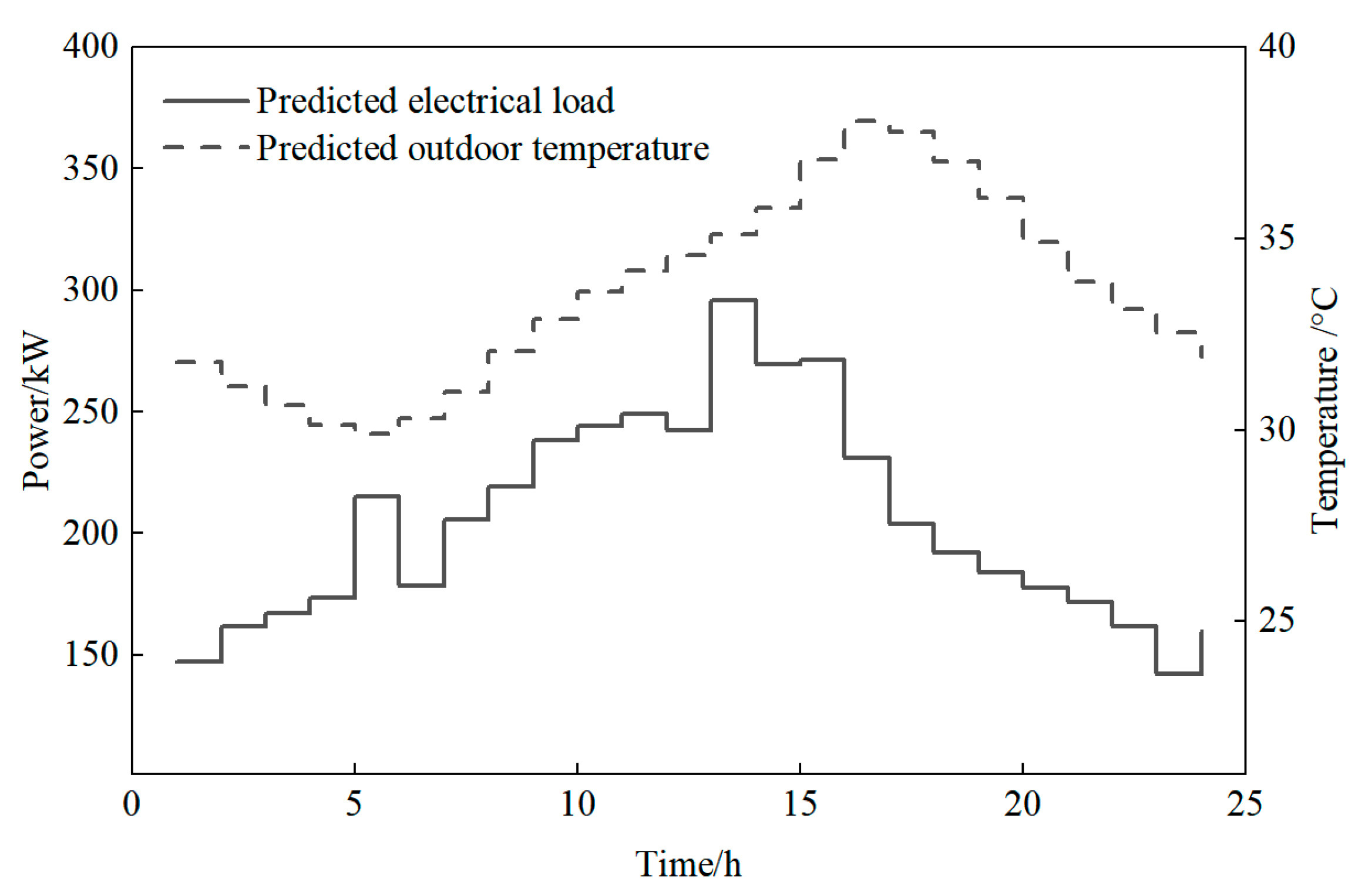
These scenarios are designed to comprehensively test the model’s robustness under diverse operating conditions. Figure 4 and Figure 5, respectively, depict the wind power and photovoltaic output curves of the Microgrid under the five typical scenarios. Meanwhile, Figure 6 shows the temporal variations of the system’s forecasted load and ambient temperature. All optimization simulations in this study were completed using the commercial solver GAMS Studio 25.1.3 (win64) with the GUROBI optimizer.

4.2. Comparison of Distributionally Robust Optimization with Other Optimization Methods

To verify the efficacy of the proposed KL divergence-based distributionally robust optimization (DRO) model, two typical benchmark models were set up for comparison: a stochastic optimization (SO) method and a traditional robust optimization (RO) process. The SO and RO models were selected as benchmarks because they represent the two most prevalent and conceptually contrasting approaches to handling uncertainty. SO relies on a fixed probability distribution and can be over-optimistic, while RO considers the worst-case scenario within a set and can be over-conservative. Comparing our DRO model against both effectively demonstrates its core value: to balance between these two extremes. In the stochastic optimization model, wind power and photovoltaic output are centered on forecast values, constructing a probability distribution with a standard deviation of 10% of the forecast value, thereby generating 10,000 initial scenarios. To reduce computational complexity, scenario reduction techniques are applied to compress them into 20 representative scenarios for optimization. The robust approach, by contrast, models solar-wind output fluctuations based on box uncertainty sets, setting 10% of the forecast value as the uncertainty boundary for simulation analysis.

As can be seen from

Table 4. Cost comparison of uncertainty treatment methods.

Model	Single-Day Operating Cost/¥
Stochastic optimization	2688.92
Robust optimization	2903.47
Distributionally robust optimization	2820.38

, the single-day working cost of stochastic optimization approaches that of the deterministic model because stochastic optimization relies on historical data to generate numerous scenarios, obtains the distribution probabilities of typical scenarios through scenario reduction, and then calculates the expected value of the objective function to ensure the financial efficiency of stochastic optimization. However, stochastic optimization heavily depends on the accurate probability distribution of uncertain parameters, neglecting the uncertainty inherent in the probability distribution itself, which results in its scheduling plan lacking sufficient robustness in practical applications. Secondly, robust optimization results in the highest single-day operating cost. Because robust optimization focuses solely on optimizing for the worst-case scenario, the robust optimization model must find an optimal solution that holds under all uncertain parameters. As a result, the optimization outcomes of the robust optimization model are the most conservative. Compared to stochastic optimization and robust optimization, distributionally robust optimization combines the strengths of both. It does not depend on the exact probability distribution of uncertain parameters but considers the uncertainty of these probability distributions. A day-ahead schedule is determined in the first stage, and adaptive adjustments are made in the second stage after uncertainty realization, continually tracking the worst-case scenario’s probability distribution. The objective function also incorporates an expected value form, ensuring partial economic efficiency of the scheduling plan while maintaining conservatism.

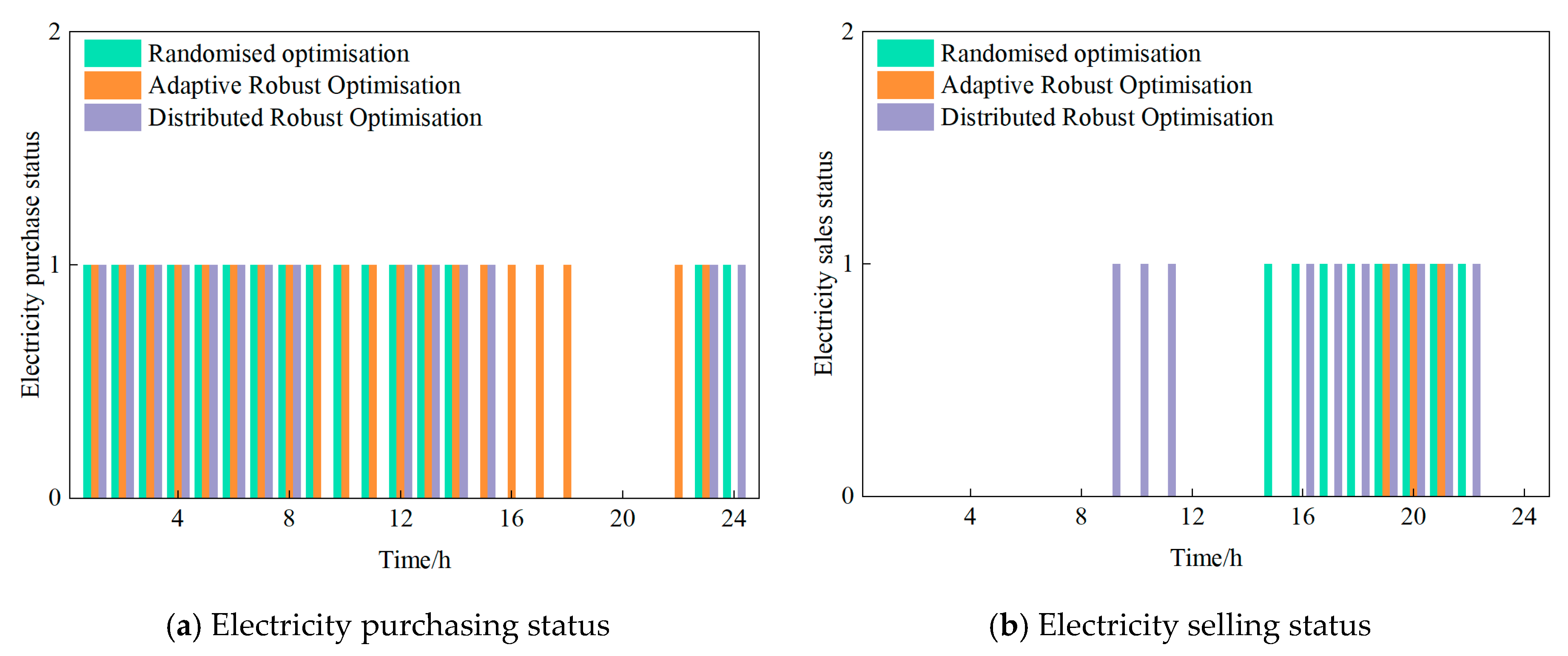
Figure 7 compares the performance of three uncertainty handling methods in the energy procuring and selling station during Stage 1. The figure uses binary variables to represent the electricity procuring and selling station: a value of 1 indicates being in the purchasing or selling state, while a value of 0 indicates no electricity purchase or sale.

The electricity purchasing status is shown in Figure 7a. The robust optimization method, due to overly considering the worst-case scenario, results in frequent electricity purchases across multiple time periods; the stochastic optimization reduces the number of purchases but, without constraints on extreme scenarios, causes the purchasing periods to be more dispersed; the distributionally robust optimization adopts a more targeted purchasing strategy, effectively reducing the number of purchases, especially during t = 10–12 h and t = 18–21 h.

The electricity selling status is shown in Figure 7b. Stochastic optimization frequently sells electricity during the high-price period from t = 16 to 21 h; robust optimization, due to its conservative strategy, sells electricity only from t = 19 to 21 h. In contrast, distributionally robust optimization increases electricity selling occurrences by three times during t = 9 to 12 h and maintains the same selling frequency as stochastic optimization from t = 16 to 21 h, indicating that the proposed distributionally robust model combines the advantages of both stochastic and robust optimization. This further validates the effectiveness of the results presented in Table 3.

4.3. Analysis of Distributionally Robust Optimization Scheduling Results

4.3.1. Analysis of Optimization Status Within the Microgrid

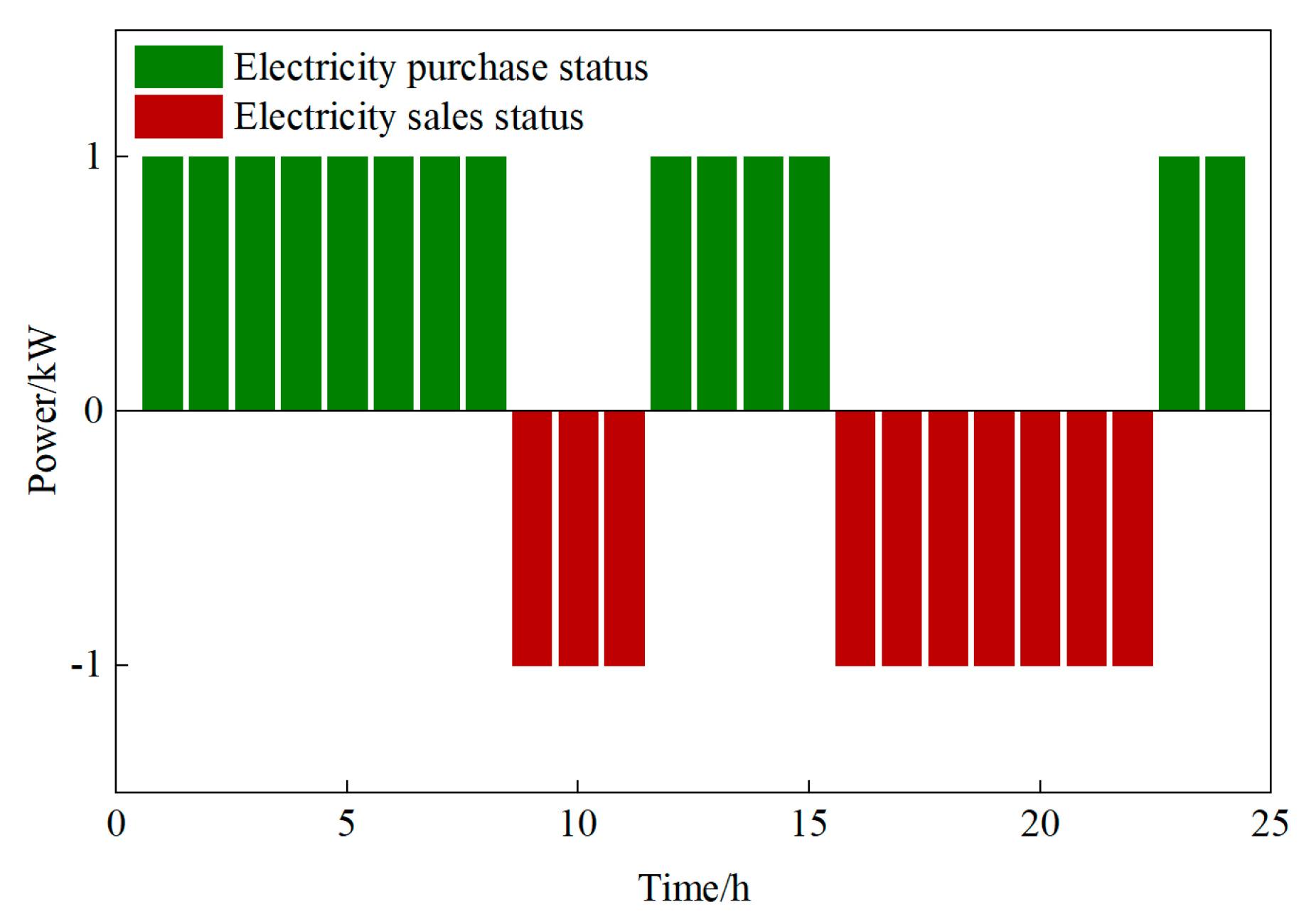
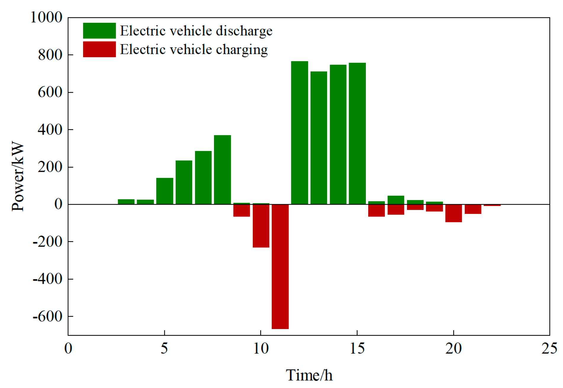
The decision variables in the initial phase of this study include the microgrid electricity purchase and sale plan, the energy storage charging and discharging schedule, and the charging and discharging power of the electric vehicle fleet. Figure 8 presents the Microgrid electricity purchase and sale plan during the first stage, while Figure 9 shows the distribution of the charging and discharging power of the electric vehicle fleet. As shown in Figure 8, the Microgrid adopts a power purchase strategy during low electricity price off-peak periods from 01:00 to 07:00, 12:00 to 13:00, and 23:00 to 24:00, and conducts power sales during peak electricity price periods from 09:00 to 11:00 and 16:00 to 22:00. This price-guided “buy low, sell high” operational strategy significantly enhances the economic efficiency of the Microgrid. Figure 9 shows that the electric vehicle cluster primarily charges during low electricity price stages such as 03:00–08:00 and 12:00–15:00, and switches to discharging mode during high electricity price stages such as 09:00–11:00. This charging and discharging behavior pattern fully validates the effectiveness of the cluster management mechanism, demonstrating that the electric vehicle fleet can intelligently respond to electricity price signals and accurately execute the optimized strategy of ‘charging during off-peak and discharging during peak’ periods.

Decisions in the next stage are made after the initial stage decisions and the realization of uncertainties, and by recourse to the probability distribution of the worst-case scenario of uncertain parameters, the expected cost is obtained, thus addressing the uncertainty of wind and photovoltaic outputs. The second stage scheduling plan is adaptively adjusted based on discrete scenarios generated from uncertain parameters. This paper analyzes the Microgrid’s optimal operation through 5 typical scenarios generated by wind power and photovoltaic output curves. It is noteworthy that the distance parameter ρ in this subsection is set to 0.01. Due to the high similarity in wind power and photovoltaic output characteristics across five typical scenarios, and consistent energy balance equations, the overall trends in microgrid optimal scheduling states are very similar.

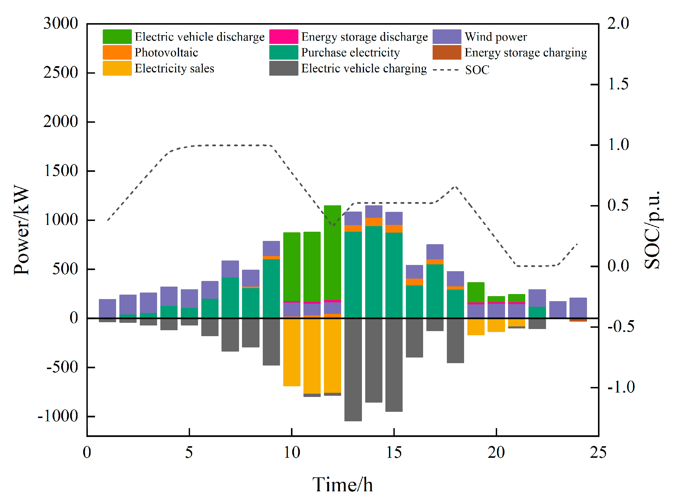
Therefore, this section analyzes the optimization results of Typical Scenario 1. Figure 10 shows the microgrid optimal scheduling results under the typical scenario. The energy storage system significantly mitigates renewable energy variability through dynamic regulation, specifically discharging at 0.28 p.u. to support system demand during the photovoltaic output low at 3 a.m., and switching to charging mode at 0.35 p.u. at noon during the photovoltaic peak to absorb surplus energy. Meanwhile, the electric vehicle cluster implements a spatiotemporal shifting strategy based on electricity price signals, with its charging load concentrated during the low-price period from 00:00 to 06:00, accounting for 72%. Additionally, it releases a discharging power of 0.15 p.u. during the evening peak from 18:00 to 20:00, effectively enhancing peak regulation capability. The external power purchase strategy further emphasizes economic efficiency by prioritizing low-cost electricity purchases at 0.12 yuan/kWh through the valley stage from 00:00 to 04:00, while completely suspending external purchases during the midday period from 12:00 to 14:00 when photovoltaic outturn is sufficient. Statistical results confirm the strong convergence properties of the robust optimization model with the risk parameter ho = 0.01 across multiple scenarios.

4.3.2. Analysis of Distributionally Robust Optimization Effects Based on KL Divergence

(1)

Robustness Analysis

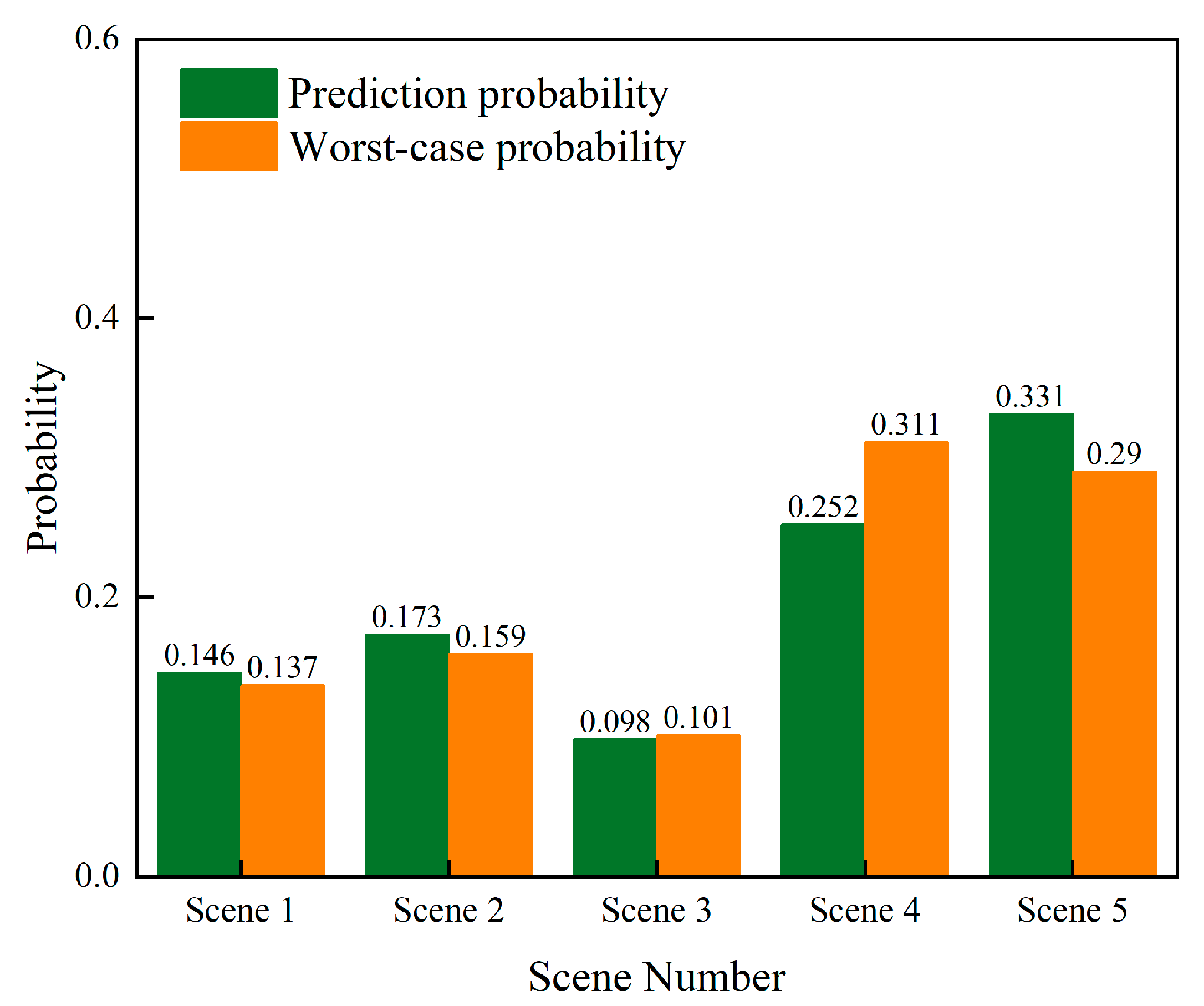
The scenario probability variations of the proposed distributionally robust optimization model are shown in Figure 11. Through the KL divergence-driven optimization mechanism, the system automatically reallocates the occurrence probabilities of each scenario: Scenario 1 decreases from 0.146 to 0.137, Scenario 2 decreases from 0.173 to 0.159, Scenario 3 slightly increases from 0.098 to 0.103, Scenario 4 rises from 0.252 to 0.311, and Scenario 5 decreases from 0.331 to 0.290. After considering uncertainty, the distributionally robust optimization model ensures the robustness of the optimization results by identifying the scenario consistent with the worst-case probability. The model automatically reduces the weights of scenarios 1, 2, and 5, which have lower operating costs, while increasing the probabilities of occurrence of the high-cost scenarios 3 and 4. Through this ‘active pessimistic’ probability adjustment mechanism, the distributionally robust optimization method effectively addresses uncertainty distributions and constructs a scheduling plan with stable performance across various scenarios, ensuring the robustness of the optimization results.

(2)

Analysis of the Impact of Changing the KL Divergence Distance Parameter on the Optimization Results

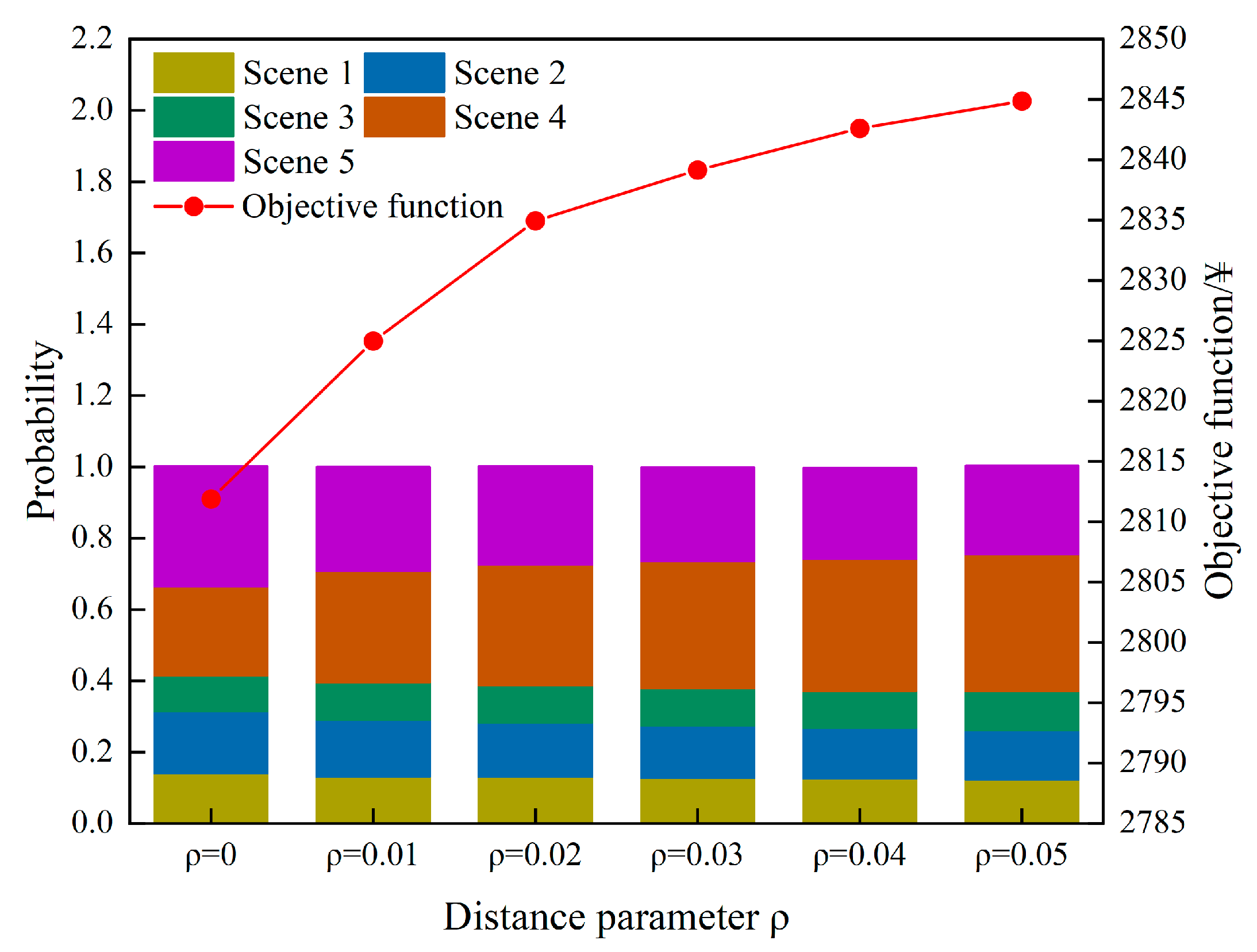
The study further examines the outcome of dissimilar KL Divergence distance parameters ρ on the optimization outcomes. As disclosed in Figure 12, when ρ = 0, distributional uncertainty is not considered, and the model degenerates into a stochastic optimization problem with five scenarios. At this point, the optimized scenario probabilities remain identical to the original distribution, and the system operating cost is 2812.47 yuan. As ρ gradually increases to 0.05, the scenario probabilities experience significant restructuring, with the worst-case probability of Scenario 1 decreasing to 0.125, Scenario 2 decreasing to 0.141, and Scenario 5 decreasing to 0.241, while the worst-case probabilities of the high-cost Scenarios 3 and 4 increase to 0.105 and 0.388, respectively. Consequently, the system operating cost rises to 2844.62 yuan. It is evident that the distance parameter ρ essentially reflects the decision maker’s level of risk aversion. An increase in its value indicates a higher degree of risk aversion by the decision maker, which in the model results in a higher optimization probability for scenarios with greater operating costs, indicating enhanced robustness against uncertainties, but also leads to increased operating costs. Therefore, in practical applications, it is necessary, based on the decision maker’s risk preferences, to collect sufficient historical data to set an appropriate distance parameter ρ.

4.3.3. Optimization Effect Analysis Based on Demand Response

To verify the economic efficacy and effectiveness of the projected demand response mode in the paper, three operating schemes are established for comparison according to the single-factor variable control principle (distance parameter ho is set to 0.01).

Scheme 1: Microgrid optimal scheduling without considering any demand response mode.

Scheme 2: Microgrid optimal scheduling reflecting shiftable demand response.

Scheme 3: Microgrid optimal scheduling considering interruptible demand response based on Scheme 2.

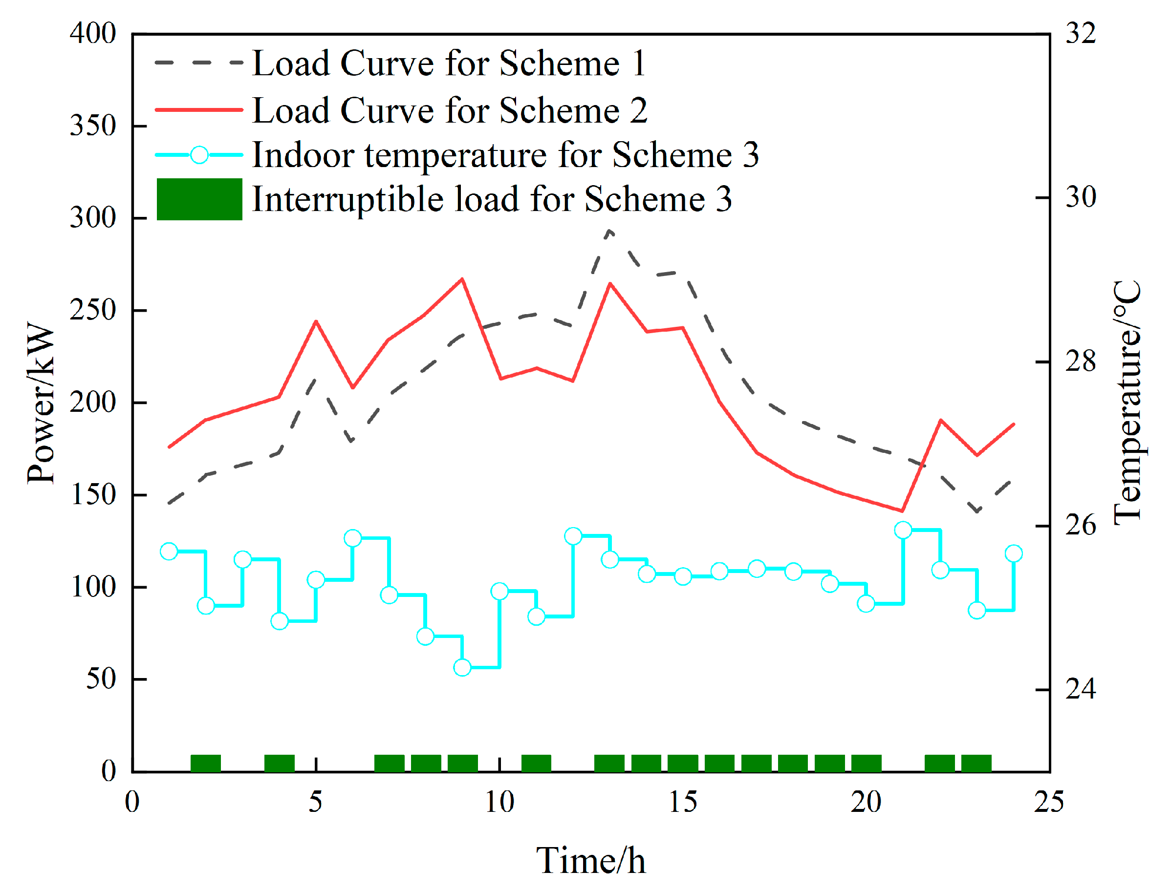
Figure 13 depicts the load variations under different schemes. The load curve of Scheme 1 shows significant fluctuations, especially during the peak period, where the load increases noticeably. This is because Scheme 1 fails to effectively shift the load and directly incurs higher electricity prices during periods of high demand, resulting in a higher single-day operating cost. In contrast, the load curve of Scheme 2 is smoother, particularly during the peak period. Load is clearly shifted from periods with higher electricity prices to those with lower prices, demonstrating that through load scheduling and response optimization, the Microgrid effectively reduces load demand during peak periods. This load adjustment not only avoids heavy load burdens during periods of high electricity prices but also reduces grid stress, thereby lowering overall operating costs. The load curve of Scheme 3 shows a mitigation of load during peak periods; however, under the indoor temperature regulation requirement (maintaining 24–26 °C), the load does not decrease as significantly as in Scheme 2. Although load demand is reduced due to interruptible load response, devices such as air conditioners must still maintain comfortable temperatures; thus, the load curve in Scheme 3 fluctuates within a certain range, resulting in a single-day operating cost slightly higher than that of Scheme 2.

Table 5. Cost comparison among different schemes.

Scheme Number	Single-Day Operating Cost/¥
Scheme 1	2886.58
Scheme 2	2799.78
Scheme 3	2820.38

presents the single-day operating costs obtained by solving the proposed distributionally robust optimization model under three schemes. It can be observed that the single-day operating cost of Scheme 2 is lower than that of Scheme 1, because under the shiftable load demand response mode, the microgrid load is shifted from periods with higher electricity prices to those with lower prices, reducing load demand during peak periods and thus lowering operating costs. The single-day operating cost of Scheme 3 is higher than that of Scheme 2 but lower than that of Scheme 1, because under the interruptible demand response mode, interruptible loads represented by air conditioners must maintain the indoor temperature within a set range (24~26 °C) to ensure human comfort; therefore, the single-day operating cost of Scheme 3 is slightly higher than that of Scheme 2.

4.4. Algorithm Convergence Results

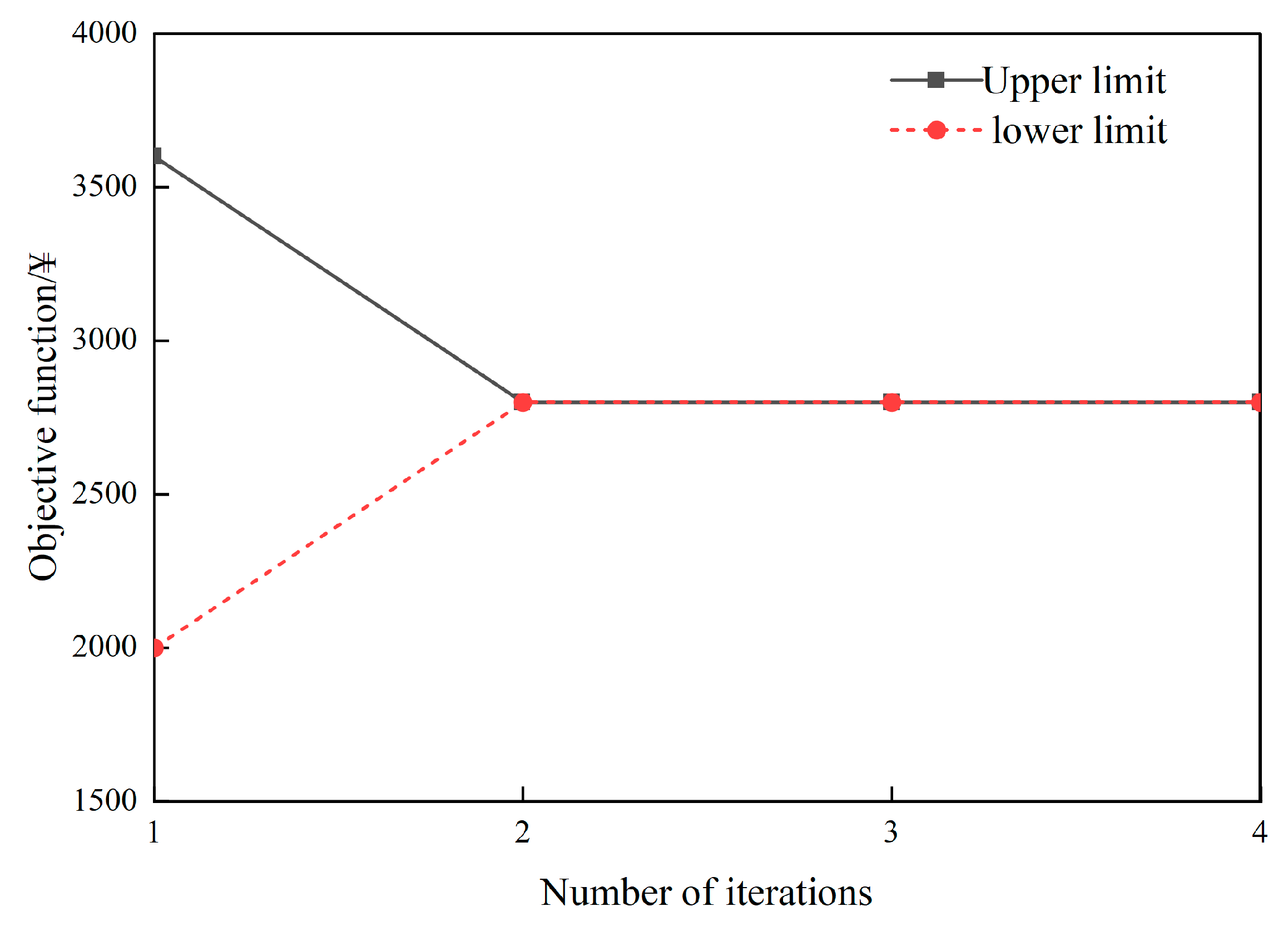
This paper decouples the distributionally robust model into a Master Problem and a Subproblem, grounded on the C&CG Algorithm, thereby dividing the optimization difficulty into complementary upper and lower bound structures. The Master Problem computation provides an upper bound estimate of the model, while solving the Subproblem generates lower bound constraints; the optimal solution is determined through iterative convergence. Meanwhile, within the Subproblem, due to the independence between the Stage 2 uncertainty variables and Stage 3 variables, the process bypasses the strong duality transformation or KKT condition application typical in traditional multi-level problems, thereby effectively simplifying the solving procedure and difficulty. The experimental data in Figure 14 show that this algorithm achieved the specified convergence accuracy within only 5.328 s of processing time, validating the method’s timeliness in practical scheduling systems and satisfying the computational demands of real-time operation.

5. Conclusions

5.1. Discussion of Findings

This study has developed a two-stage distributionally robust optimization (DRO) model for microgrids that leverages flexible demand-side resources to address renewable generation uncertainty. The core findings and their scholarly implications are summarized as follows:

(1)

The proposed DRO model demonstrates a superior balance between economy and robustness. It achieves a 2.86% reduction in daily operating cost compared to robust optimization, while remaining within 4.88% of the cost of stochastic optimization. This performance substantiates the model’s key advantage: by hedging against the worst-case probability distribution rather than a deterministic worst-case scenario, it effectively mitigates the over-conservatism inherent in traditional robust optimization [22], while providing greater resilience to distributional errors than stochastic optimization.

(2)

The model successfully integrates the merits of both stochastic and robust optimization paradigms. Central to this integration is the KL divergence parameter ρ, which provides system operators with a direct and mathematically transparent mechanism to calibrate the trade-off between conservatism and cost. An increase in ρ, indicative of greater risk aversion, shifts the probability weight towards higher-cost scenarios, thereby systematically enhancing operational robustness.

The incorporation of interruptible and transferable demand response modes is confirmed as a critical driver of system efficiency. These mechanisms effectively optimize load scheduling, curtail peak demand, and consequently reduce overall scheduling costs. The efficacy of coordinating such flexible resources, including electric vehicle clusters, aligns with and reinforces the findings of prior studies [23], and is further supported by recent research on low-carbon scheduling of AC/DC microgrids [24,25], differentiated demand response [26], energy storage support [27], renewable uncertainty handling [28], and the integration of EVs [29,30,31,32], underscoring their indispensable role in future energy systems.

5.2. Limitations

This study has several limitations. First, the use of linear models for components like energy storage may not capture nonlinear dynamics under all operating conditions. Second, the computational burden, though mitigated by the C&CG algorithm, could challenge real-time applications in very large-scale systems. Finally, the model’s performance is contingent on the representativeness of historical data used to construct the ambiguity set.

5.3. Future Work

Future research will focus on integrating nonlinear component models and developing more efficient algorithms to enhance scalability. The framework will be extended to multi-microgrid systems to investigate cooperative scheduling and energy trading. Furthermore, we will explore data-driven techniques, such as generative models, to construct ambiguity sets directly from data, reducing reliance on predefined distributions and improving adaptability.

References

1. Ye, X.; Wang, C.; Shi, Z. Analysis of High Proportion Renewable Energy Integration Abroad and Recommendations for Sustainable Development of New Energy in China. China Electr. Power 2025, 58, 137. [Google Scholar] [CrossRef]
2. Georgia, K.; Szábo, S.; Jäger-Waldau, A. Powering Up to Cool Down Climate Change: Tripling Renewable Energy to Meet COP28 Pledge in the EU. In Proceedings of the 2024 IEEE 52nd Photovoltaic Specialist Conference (PVSC), Seattle, WA, USA, 9–14 June 2024. [Google Scholar] [CrossRef]
3. Zhang, Z.; Wu, Y.; Li, X. Microgrid Islanded Operation Strategy Supported by Aggregated Charging and Discharging of Electric Vehicles. Mod. Electr. Power 2025, 42, 1–12. [Google Scholar] [CrossRef]
4. Zuo, J.; Zhong, Y.; Bao, B. Multi-Objective Optimization Model for Power Grid Operation Scheduling Considering the Uncertainty of New Energy. Grid Clean Energy 2025, 41, 152–158. Available online: https://epjournal.csee.org.cn/zh/article/129939526/ (accessed on 28 November 2025).
5. Chen, M.; Geng, J.; Zhao, Y. Weekly Operation Strategy of Electric-Hydrogen Coupled Microgrid Based on Two-stage Stochastic Optimization. China Electr. Power 2024, 58, 82. [Google Scholar] [CrossRef]
6. Wei, B.; Han, X.; Li, W. Multi-timescale stochastic optimization scheduling strategy for AC-DC hybrid microgrids incorporating multi-scenario analysis. High Volt. Eng. 2020, 46, 2359–2369. [Google Scholar] [CrossRef]
7. Hu, H. Research on Optimal Scheduling of Multi-Form Microgrid Clusters Considering Uncertainty Under the New Power System. Ph.D. Theis, North China Electric Power University, Beijing, China, 2024. [Google Scholar] [CrossRef]
8. Liu, J.; Wu, R.; Yao, X. Joint Bidding Strategy of Compressed Air Energy Storage and Wind Power Based on Stochastic Dual Dynamic Integer Programming. South. Power Grid Technol. 2024, 18, 127–137. [Google Scholar] [CrossRef]
9. Ma, Y. Research on Low-Carbon Economic Dispatch of Microgrids Based on Robust Optimization. Ph.D. Thesis, Taiyuan University of Technology, Taiyuan, China, 2023. [Google Scholar] [CrossRef]
10. Chen, Y.; Lou, G.; Ji, L.; Wang, P.; Jing, X.; Huang, J. Adaptive Two-Stage Robust Optimization Scheduling Method for Wind-Solar-Storage Based on the i-C&CG Algorithm. J. Electr. Power Sci. Technol. 2025, 40, 141–153. [Google Scholar] [CrossRef]
11. Liu, Y.; Guo, L.; Wang, C. Two-stage robust optimization economic dispatch method for microgrid. Proc. Chin. Soc. Electr. Eng. 2018, 38, 4013–4022+4307. [Google Scholar] [CrossRef]
12. Wang, Z.; Hou, H.; Zhao, B.; Zhang, L.; Shi, Y.; Xie, C. Risk-averse stochastic capacity planning and P2P trading collaborative optimization for multi-energy microgrids considering carbon emission limitations: An asymmetric Nash bargaining approach. Appl. Energy 2024, 357, 122505. [Google Scholar] [CrossRef]
13. Wang, L.; Wang, Z.; Li, Z.; Yang, M.; Cheng, X. Distributed optimization for network-constrained peer-to-peer energy trading among multiple microgrids under uncertainty. Int. J. Electr. Power Energy Syst. 2023, 149, 109065. [Google Scholar] [CrossRef]
14. Shen, Y.; Zhai, J.; Kang, Z.; Zhao, B.; Gao, X.; Li, Z. Distributionally robust chance-constrained energy management for island DC microgrid with offshore wind power hydrogen production. Energy 2025, 316, 134570. [Google Scholar] [CrossRef]
15. Wu, Y. Distributionally Robust Low-carbon Economic Optimal Scheduling for Integrated Energy Microgrid. Ph.D. Thesis, Hunan University, Changsha, China, 2023. [Google Scholar] [CrossRef]
16. Xie, L.; Tang, Z.; Huang, X. Bilevel Dynamic Distribution Network Reconfiguration Considering Uncertainties of Distributed Generation and Electric Vehicles. Electr. Power Syst. Prot. Control. 2020, 48, 1–11. [Google Scholar] [CrossRef]
17. Yuan, S.; He, Y.; Dai, Z. Modeling of Temporal Correlation Polyhedral Uncertainty of Wind Power and Robust Unit Commitment Optimization. Acta Energiae Solaris Sin. 2020, 41, 293–301. [Google Scholar]
18. Zhang, X.; Kuang, Y.; Zhou, L. Collaborative Optimal Scheduling of Active Distribution Network and Multiple Microgrids Considering Wind and Solar Uncertainties. Water Resour. Hydropower Technol. 2025, 1–10. Available online: https://link.cnki.net/urlid/10.1746.tv.20250417.1730.002 (accessed on 28 November 2025).
19. Lu, J.; Huang, D.; Ren, H. Data-driven source-load robust optimal scheduling of integrated energy production unit including hydrogen energy coupling. Glob. Energy Interconnect. 2023, 6, 375–388. [Google Scholar] [CrossRef]
20. Meng, Y.; Yin, Z.; Zhang, Y.; Zhu, R. Distributed collaborative scheduling of multiple microgrids based on distributionally robust non-zero-sum games. J. Electr. Power Syst. Autom. 2025, 1–12. [Google Scholar] [CrossRef]
21. Jiang, X.; Bao, Z.; Yu, M.; Guo, C.; Guo, Y.; Wang, J. Distributionally robust multi-stage planning of integrated energy systems for industrial parks considering source and load uncertainties. Power Constr. 2025, 46, 99–112. [Google Scholar] [CrossRef]
22. Wei, M.; Wu, Y.; Li, Y. Day-Ahead Economic Operation Model and Solution Method for Microgrids Based on Distributionally Robust Optimization. Proc. Chin. Soc. Electr. Eng. 2022, 34, 81–90. [Google Scholar] [CrossRef]
23. Ge, L.; Fan, Y.; Lai, J.; Sun, H.; Zhang, Y. Artificial Intelligence-Enabled Microgrid Optimal Operation Technology for a Low-Carbon Economy. High Volt. Technol. 2023, 49, 2219–2238. [Google Scholar] [CrossRef]
24. Yang, X.; Zhang, W.; Zou, W.; Li, B.; Chen, X. Low-Carbon Optimal Scheduling of AC-DC Hybrid Microgrids Considering Green Certificate Trading and Carbon Emission Constraints. Intell. Power 2025, 53, 9–16. [Google Scholar] [CrossRef]
25. Li, X.; Chen, Y.; Li, H.; Liu, L.; Huang, J.; Guo, P. Two-Stage Robust Optimization Low-Carbon Economic Dispatch of Electric-Thermal Integrated Energy Systems Considering Carbon Trading. Power Constr. 2024, 45, 58–69. [Google Scholar] [CrossRef]
26. Peng, C.; Zhang, J.; Chen, L. Coordinated Optimal Scheduling of Microgrid Sources, Loads, and Storage Considering Differentiated Demand Response. Electr. Power Autom. Equip. 2020, 40, 1–7. [Google Scholar] [CrossRef]
27. Yan, Z.; Li, L.; Yang, P. Microgrid Optimal Scheduling Strategy Considering Networked Energy Storage Support Capability. China Electr. Power 2025, 58, 103–110. [Google Scholar] [CrossRef]
28. Sun, X.; Liu, J.; Zhao, D. Multi-Energy Microgrid Scheduling Optimization Model Based on Renewable Energy Uncertainty. Science. Technol. Eng. 2020, 20, 14523–14532. [Google Scholar]
29. Rezaei, N.; Khazali, A.; Mazidi, M.; Ahmadi, A. Economic energy and reserve management of renewable-based microgrids in the presence of electric vehicle aggregators: A robust optimization approach. Energy 2020, 201, 117629. [Google Scholar] [CrossRef]
30. Kuang, H.; Xu, Y.; Li, Z. Microgrid Optimal Scheduling Including Electric Vehicles Based on an Improved Scarab Optimization Algorithm. Power Sci. Eng. 2024, 40, 10–17. [Google Scholar] [CrossRef]
31. Xiao, C.; Zhang, K.; Feng, J. Hierarchical Optimal Scheduling of an Independent Wind/Solar/Diesel Microgrid Incorporating Electric Vehicle Charging Stations. J. Tianjin Univ. Technol. 2022, 41, 61–74. [Google Scholar] [CrossRef]
32. Lu, Y.; Yin, L.; Xu, G. Multi-objective Optimization of Combined Cooling, Heating, and Power Microgrid Based on Incentive Demand Response. South. Power Grid Technol. 2025, 1–13. [Google Scholar] [CrossRef]
Figure 1. Schematic Diagram of the Microgrid System Structure.
Energies 18 06516 g001
Figure 2. Two-stage distributionally robust optimization model of the Microgrid and its hierarchical frame.
Energies 18 06516 g002
Figure 3. Microgrid Two-stage Distributionally Robust Solution Process. (A complete list of all notations is provided in Appendix A for reference).
Energies 18 06516 g003
Figure 4. Wind Power Output of the Microgrid under 5 Typical Scenarios.
Energies 18 06516 g004
Figure 5. Photovoltaic Output of the Microgrid under 5 Scenarios.
Energies 18 06516 g005
Figure 6. Temporal Variation of Forecasted Electrical Load and Outdoor Temperature.
Energies 18 06516 g006
Figure 7. Comparison of microgrid electricity purchasing and selling statuses under different uncertainty methods.
Energies 18 06516 g007
Figure 8. Electricity purchase and sale plan for the initial stage.
Energies 18 06516 g008
Figure 9. Charging and Discharging Power of All 200 Electric Vehicles.
Energies 18 06516 g009
Figure 10. Scenario 1 Microgrid Optimal Scheduling Conditions.
Energies 18 06516 g010
Figure 11. Scenario Probability Variation.
Energies 18 06516 g011
Figure 12. Different distance parameters ρ Influence.
Energies 18 06516 g012
Figure 13. Load variation curves under different schemes.
Energies 18 06516 g013
Figure 14. Convergence curve of the model based on the C&CG Algorithm.
Energies 18 06516 g014