Enhancing Photovoltaic Power Forecasting via Dual Signal Decomposition and an Optimized Hybrid Deep Learning Framework

Abstract

Accurate prediction of photovoltaic power generation is a pivotal factor for enhancing the operational efficiency of electrical grids and facilitating the stable integration of solar energy. This study introduces a holistic forecasting framework that achieves seamless integration of dual-stage decomposition, deep learning architectures, and an advanced metaheuristic algorithm, thereby significantly improving the prediction precision of PV power generation. Initially, the raw PV power sequences are processed using Improved Complete Ensemble Empirical Mode Decomposition with Adaptive Noise (ICEEMDAN) to capture multi-scale temporal characteristics. The derived components are subsequently categorized into high-, medium-, and low-frequency groups through K-means clustering to manage complexity. To address residual noise and non-stationary behaviors, the high-frequency constituents are further decomposed via Variational Mode Decomposition (VMD). The refined subsequences are then input into a TCN_BiGRU_Attention network, which employs temporal convolutional operations for hierarchical feature extraction, bidirectional gated recurrent units to model temporal correlations, and a multi-head attention mechanism to prioritize influential time steps. For hyperparameter optimization of the forecasting model, an Improved Crested Porcupine Optimizer (ICPO) is developed, integrating Chebyshev chaotic mapping for initialization, a triangular wandering strategy for local search, and Lévy flight to strengthen global exploration and accelerate convergence. Validation on real-world PV datasets indicates that the proposed model attains a Mean Squared Error (MSE) of 0.3456, Root Mean Squared Error (RMSE) of 0.5879, Mean Absolute Error (MAE) of 0.3396, and a determination coefficient (R²) of 99.59%, surpassing all benchmark models by a significant margin. This research empirically demonstrates the efficacy of the dual decomposition methodology coupled with the optimized hybrid deep learning network in elevating both the accuracy and stability of predictions, thereby offering a reliable and stable forecasting framework for PV power systems.

1. Introduction

As a critical component of renewable energy systems, photovoltaic power generation plays an increasingly vital role in the global transformation of energy infrastructure [1]. Nevertheless, PV power output exhibits significant variability and instability due to its dependence on diverse meteorological factors such as atmospheric temperature, relative humidity, wind speed, directional airflow, and solar irradiance, among others [2]. These inherent fluctuations introduce considerable complexities for maintaining grid stability, formulating effective dispatch strategies, and executing electricity market operations [3]. Consequently, high-accuracy forecasting of PV power generation enables more efficient allocation of grid resources, lowers peak-shaving expenses, and improves renewable energy absorption capacity, thereby emerging as a pivotal research domain within the energy sector [4].

Traditional methodologies for photovoltaic power prediction are generally classified into two main streams: physical model-based approaches and statistical data-driven techniques [5]. Physical approaches formulate mathematical representations by combining numerical weather prediction (NWP) information with the inherent physical characteristics of PV systems. Since this methodology does not require historical operational records, it proves especially advantageous for newly commissioned power stations [6]. However, the predictive accuracy of such methods is heavily dependent on the precision of NWP inputs and the comprehensiveness of the underlying physical representations [7]. In contrast, statistical techniques rely on historical power generation data to establish predictive models, employing conventional time-series algorithms such as Auto Regressive Integrated Moving Average (ARIMA) [8], and Auto Regressive Moving Average (ARMA) [9], among others. Despite their widespread application, these conventional methods exhibit notable limitations in modeling nonlinear relationships and processing high-dimensional datasets. Specifically, physical models demonstrate high sensitivity to the quality and resolution of meteorological data, whereas statistical approaches often fail to accurately represent complex dynamic behaviors under rapidly changing weather conditions. These inherent shortcomings have accelerated the adoption of machine learning strategies in PV forecasting, thereby promoting a fundamental transition from traditional modeling paradigms toward data-driven analytical frameworks [10].

The proliferation of big data technologies and enhanced accessibility of high-quality datasets have led to a growing utilization of machine learning techniques in photovoltaic power forecasting [11]. Methods including Support Vector Machines (SVM) [12], Random Forest (RF) [13], and gradient boosting tree variants such as XGBoost [14] and LightGBM [15] demonstrate a pronounced ability to autonomously capture intricate nonlinear interactions and multivariate coupled characteristics from historical records, thereby substantially improving prediction accuracy [16]. These data-driven algorithms exhibit clear advantages over conventional approaches, particularly in recognizing complex patterns and processing high-dimensional datasets, effectively addressing numerous constraints inherent in traditional forecasting frameworks. Through adaptive learning mechanisms, machine learning models uncover latent data patterns while maintaining considerable robustness and generalization performance [17]. Nonetheless, with the escalating complexity of prediction scenarios and continuous expansion of data volumes, these methods increasingly reveal limitations in modeling long-term temporal dependencies and capturing sophisticated spatiotemporal relationships [18]. This identified gap has subsequently accelerated the development and deployment of more advanced deep learning architectures within the PV forecasting domain [19].

Deep learning architectures have driven substantial advancements in photovoltaic power forecasting, largely attributable to their superior capabilities in automated feature representation and sequential pattern modeling [20]. Particularly, recurrent neural network variants like Long Short-Term Memory (LSTM) [21] and gated recurrent unit (GRU) [22] excel at modeling temporal relationships across extended time horizons and have shown exceptional efficacy in ultra-short-term prediction scenarios [23]. Through sophisticated gating mechanisms that dynamically regulate information flow—selectively preserving relevant features while discarding redundant information—these models effectively alleviate the persistent challenges of gradient vanishing and explosion that plague conventional recurrent networks [6].

In pursuit of augmented predictive capabilities in deep learning frameworks, numerous optimization and integration methodologies have been introduced. One prominent strategy involves the coupling of variational mode decomposition (VMD) with gated recurrent units refined by metaheuristic optimization techniques. This hybrid approach dissects raw photovoltaic data into multiple intrinsic mode functions (IMFs) spanning distinct frequency bands, effectively attenuating non-stationary characteristics in the original sequences. Concurrently, the implementation of intelligent optimization algorithms for comprehensive hyperparameter configuration significantly enhances the development of more resilient forecasting architectures [24]. As deep learning methodologies continue to evolve, composite structures incorporating temporal convolutional networks (TCN) [25], bidirectional gated recurrent units (BiGRU) [26], and attention mechanisms have manifested pronounced superiority. The prototypical TCN-BiGRU-Attention framework employs a staged processing pipeline: initially, the TCN component utilizes dilated convolutional operations to derive multi-scale temporal attributes from input sequences; subsequently, the BiGRU module models both forward and backward temporal relationships within the extracted features; ultimately, the attention component dynamically prioritizes salient temporal information through adaptive weighting of BiGRU outputs, synthesizing the final forecast [27]. This synergistic architecture capitalizes on the extended temporal dependency modeling of TCN, the bidirectional context encoding of BiGRU, and the discriminative feature emphasis enabled by attention, collectively elevating both predictive precision and operational stability [28].

This paper presents a hybrid forecasting framework for short-term photovoltaic power prediction, built upon a dual-stage decomposition architecture. The proposed methodology initiates with the application of Improved Complete Ensemble Empirical Mode Decomposition with Adaptive Noise (ICEEMDAN) to disassemble the original PV power sequence into constituent components. Subsequent computation of sample entropy for these components enables their classification into high-, medium-, and low-frequency categories through K-means clustering. The highest-frequency cluster then undergoes secondary decomposition via Variational Mode Decomposition (VMD) to further refine its characteristics. Each resulting subcomponent is processed through a TCN_BiGRU_Attention network for individual prediction, with the final PV power forecast obtained through systematic reconstruction of all subsequence predictions. Experimental validation confirms the superior predictive accuracy of this integrated approach compared to conventional forecasting techniques. The principal contributions of this research are delineated as follows:

• A novel hybrid forecasting methodology is introduced, integrating ICEEMDAN, VMD, TCN, BiGRU, Attention mechanism, and ICPO optimization. The TCN_BiGRU_Attention composite architecture demonstrates enhanced capability in capturing long-range temporal dependencies within power sequences while leveraging attention mechanisms to accentuate critical temporal features, thereby effectively modeling complex nonlinear relationships inherent in PV power data.
• A comprehensive feature extraction strategy is implemented through the synergistic application of ICEEMDAN, K-means clustering, and VMD techniques. This multi-layered decomposition approach facilitates thorough exploitation of data characteristics across different frequency domains, substantially improving the model’s predictive performance.
• Significant enhancements to the Crested Porcupine Optimizer (CPO) are achieved through incorporating Chebyshev Chaotic Mapping, Triangular Wandering Strategy, and Lévy Flight mechanisms. These modifications promote superior initial population distribution within the search space, consequently accelerating the convergence rate of the TCN_BiGRU_Attention model during training.

2. Method

2.1. Improved Complete Ensemble Empirical Mode Decomposition with Adaptive Noise (ICEEMDAN)

As an enhanced version of the conventional Ensemble Empirical Mode Decomposition technique, the Improved Complete Ensemble Empirical Mode Decomposition with Adaptive Noise (ICEEMDAN) demonstrates substantial methodological progress [29]. This advanced algorithm introduces adaptively scaled noise at each decomposition stage, effectively suppressing mode mixing artifacts while improving the frequency-domain distinctness of the extracted intrinsic mode functions (IMFs). Through iterative ensemble averaging operations, the method diminishes noise interference in the final components, consequently strengthening the decomposition’s overall robustness. Additionally, ICEEMDAN implements a fully adaptive noise-injection mechanism that dynamically modulates noise amplitudes across iterations, achieving superior spectral separation performance with reduced computational requirements. These characteristics collectively ensure markedly enhanced decomposition precision, rendering the approach particularly suitable for time-frequency analysis tasks in applications ranging from fault detection to signal purification. Such technical advantages significantly elevate its practical utility in engineering implementations. The operational workflow of the ICEEMDAN methodology comprises the following sequential steps.

Firstly, gaussian white noise $E_1({\omega }^{(i)})$ is added to the initial signal $s$, which is obtained:

$$s^{(i)}=s+{\beta }_0{E}_1({\omega }^{(i)})$$

(1)

where ${\omega }^{(i)}$ denotes the $ith$ white noise being added; $E_k(\cdot )$ denotes the $kth$ $IMF$ component of the EMD decomposition of a signal being sought.

Secondly, the original time series is decomposed using the ICEEMDAN algorithm to obtain the first $IMF$ component:

$$\left\{\begin{array}{l}{r}_1={\displaystyle \frac{1}{I}}{\displaystyle \sum _{i=1}^{I}M(x^{(i)})}\\ c_1 = x - r_1\end{array}\right.$$

(2)

where $r_1$ denotes the first-order residual; $c_1$ denotes the first $IMF$ value.

Then, continue to calculate the second $IMF$ component:

$$\left\{\begin{array}{l}{r}_2={\displaystyle \frac{1}{I}}{\displaystyle \sum _{i=1}^{I}M\left\{r_1+{\beta }_1{E}_2({\omega }^{(i)})\right\}}\\ c_2=r_1-r_2\end{array}\right.$$

(3)

where $r_2$ denotes the first-order residual; $c_2$ denotes the second $IMF$ value.

Finally, calculate the $kth$ $IMF$ component:

$$\left\{\begin{array}{l}{r}_k={\displaystyle \frac{1}{I}}{\displaystyle \sum _{i=1}^{I}M\left\{r_{k-1}+{\beta }_{k-1}{E}_k({\omega }^{(i)})\right\}}\\ c_k=r_{k-1}-r_k\end{array}\right.$$

(4)

where $k=2,3,\dots ;$$r_k$ denotes the $kth$ order residual; $c_k$ denotes the $kth$ $IMF$ value, ${\beta }_k={\epsilon }_{k}std(r_k), k\ge 1$, ${\beta }_0={\epsilon }_{0}std(x)/std(E_1({\omega }^{(i)}))$, $\epsilon$ denotes the noise figure.

2.2. Varational Mode Decomposition (VMD)

Variational Mode Decomposition (VMD), as an emerging signal processing technique [30] demonstrates multiple distinctive merits in analyzing non-stationary sequences. The method operates by solving a constrained variational optimization problem, through which it systematically segregates complex signals into a finite collection of Intrinsic Mode Functions (IMFs) with specific central frequencies. This decomposition mechanism thereby enables high-resolution time-frequency representations of non-stationary signals. Another crucial feature lies in its incorporation of penalty terms and reconstruction constraints during the decomposition process, which enhances sparsity in the resultant modes and helps mitigate the mode overlap problem frequently observed in alternative decomposition methods. Consequently, the precision of signal decomposition and the quality of reconstructed signals are substantially improved. Additionally, VMD is computationally effective, permitting swift processing that aligns well with real-time implementation requirements. The method also maintains reliable performance under noisy environments due to its inherent resistance to interference. Furthermore, VMD’s self-adaptive capability enables automatic determination of the optimal number of decomposition modes according to signal attributes, thus ensuring that the derived components faithfully represent the inherent structural characteristics of the original signal.

VMD decomposes the input historical photovoltaic power generation sequence $f\left(t\right)$ into $K$ modal $\left\{u_k\right\}=\left\{u_1\left(t\right),\dots u_K\left(t\right)\right\}$. The method requires a finite bandwidth for each mode around its center frequency ${\omega }_k$ such that the sum of the estimated bandwidths of all modes is minimized and the variational optimization model is:

$$\left\{\begin{array}{l}\min {\displaystyle \sum _{k=1}^K{\parallel \partial \left\{\left[\left(\delta \left(t\right)+j/\left(\pi t\right)\right)\ast u_k\left(t\right)\right]e^{-j{\omega }_{k}t}\right\}\parallel }_2^2}\\ s.t.{\displaystyle \sum _{k=1}^K{u}_k\left(t\right)=f\left(t\right)}\end{array}\right.$$

(5)

where $\delta \left(t\right)$ is the unit pulse function at moment $t$, $j$ is an imaginary unit,${\partial }_t$ is the partial derivative of the function with respect to $t$, $\left\{{\omega }_k\right\}=\left\{{\omega }_1,\dots ,{\omega }_K\right\}$ is the set of center frequencies, and ${‖\cdot ‖}_2^2={{\displaystyle \underset{R}{\int }\left|\cdot \right|}}^{2}dt$. In the above model, the constraint is that the sum of the $K$ modal functions is equal to the input wind speed sequence $f\left(t\right)$.

2.3. K-Means Clustering

The K-means clustering technique, widely known as the centroid-based partitioning algorithm [31], operates as an unsupervised learning approach that partitions data objects into homogeneous groups according to specified feature dimensions. This method maximizes intra-cluster similarity while minimizing inter-cluster resemblance through an iterative optimization process.

The fundamental workflow of the K-means algorithm proceeds through the following operational stages:

Step 1: Initialize the target dataset and specify the predetermined number of clusters ($k$).

Step 2: Randomly select K observations from the input data as initial cluster centroids.

Step 3: Compute the proximity between each data point and all current cluster centroids, then assign every sample to its nearest cluster. For two n-dimensional vectors, say: $X\left(x_1,x_2,\dots x_n\right)$ and $Y\left(y_1,y_2\dots y_n\right)$, their dissimilarity is measured using the Euclidean Distance metric:

$$d=\sqrt{{\displaystyle {\sum }_{k=1}^n{\left(x_k-x_k\right)}^2}}$$

(6)

Step 4: Recalculate cluster centroids by averaging all member points within each partition. The iterative process terminates when the change in the within-cluster sum of squares falls below a predefined threshold, indicating centroid stabilization. Otherwise, the algorithm returns to Step 3 for further refinement.

2.4. Temporal Convolutional Network (TCN) Algorithm

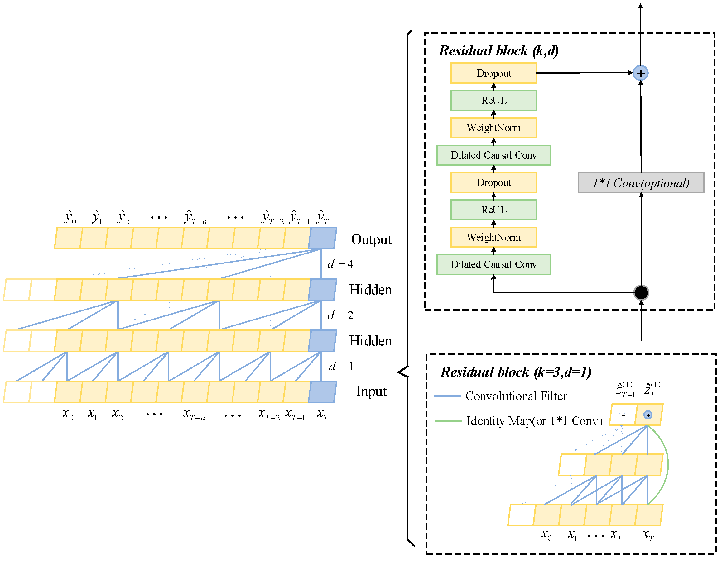
The Temporal Convolutional Network (TCN) constitutes a specialized deep learning architecture tailored for sequential data analysis [32]. Its conceptual foundation lies in adapting the feature extraction principles of conventional Convolutional Neural Networks (CNNs) to temporal contexts, utilizing convolutional operations to identify and model patterns within sequential inputs. A distinctive advantage of TCN is its inherent support for parallel computation, which grants it particular efficacy in handling extended sequential datasets. Among its fundamental constituents are causal convolutions, dilated convolutional structures, and residual connections.

Assuming the input of the $i\mathrm{th}$ residual block is $X^i$ and the output is $X^{i+1}$, the expression is:

$$X^{i+1}=Activation(X^i+F(X^i))$$

(7)

where $Activation$ denotes the activation function; $F(x)$ denotes the residual block operation. The model framework of the TCN is shown in Figure 1.

2.5. Bidirectional Gated Recurrent Unit (BiGRU)

The Gated Recurrent Unit (GRU) represents a streamlined variant of the Long Short-Term Memory (LSTM) architecture [33], designed to maintain comparable temporal modeling capabilities while offering greater structural simplicity and computational efficiency. This recurrent network employs a consolidated gating mechanism that effectively mitigates issues of gradient instability and long-term dependency modeling encountered in standard Recurrent Neural Networks (RNNs). Specifically, the GRU framework incorporates two fundamental gating components: a reset gate and an update gate. The reset gate regulates the retention degree of prior hidden states, while the update gate governs the integration of new inputs with historical information. Through these coordinated gating operations, the model achieves enhanced capacity to preserve critical temporal features and effectively capture both immediate and extended dependencies within sequential data. The mathematical formulation of the GRU cell is defined as follows:

$$z_t=\sigma \left(W_{iz}{x}_t+b_{iz}+W_{hz}{h}_{t-1}+b_{ht}\right)$$

(8)

$$r_t=\sigma \left(W_{ir}{x}_t+b_{ir}+W_{hr}{h}_{t-1}+b_{hr}\right)$$

(9)

$$h_t=\tanh \left(W_{in}{x}_t+b_{in}+r_t\odot \left(W_{hn}{h}_{t-1}+b_{hn}\right)\right)$$

(10)

$$h_t=\left(1-z_t\right)\odot h_{t-1}+z_t\odot h_t$$

(11)

where $h_{t-1}$ denotes the hidden state at time $t-1$; $x_t$ denotes the input at time $t$; $\sigma$ denotes the sigmoid activation function; $r_t$ denotes the reset gate; $z_t$ denotes the update gate; $h_{t-1}$ denotes the candidate hidden state; $h_t$ denotes the final hidden state; $W$ denotes the coefficient matrix; $\odot$ denotes the Hadamard product; $b$ denotes the bias parameter.

The Bidirectional Gated Recurrent Unit (BiGRU) represents an enhanced recurrent architecture that incorporates both forward and backward processing of sequential information. This dual-directional design enables the network to simultaneously incorporate preceding and subsequent contextual information, thereby effectively capturing both immediate contextual cues and extended temporal relationships through integrated feature splicing from bidirectional hidden states. Consequently, BiGRU demonstrates superior capability in representing complex temporal patterns and modeling sophisticated dependencies within sequential data structures.

2.6. Multi-Head Attention Mechanism

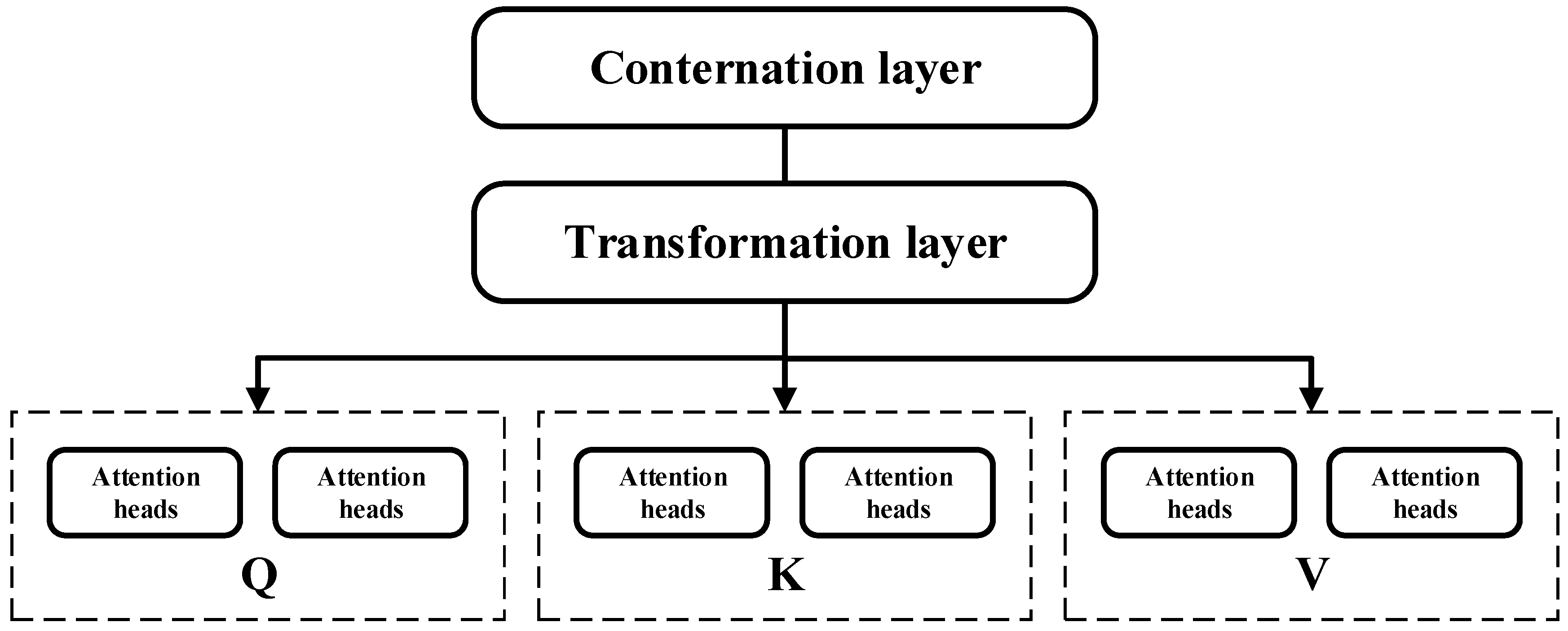
The Multi-Head Attention (MHA) mechanism serves as a foundational component in Transformer-based architectures [34], constituting a significant extension beyond the standard self-attention framework. By parallelly employing multiple independently parameterized attention heads, the model gains the capacity to jointly attend to information from distinct representational subspaces, thereby collectively enhancing its expressive power and feature discriminability.

A detailed structural representation of the multi-head self-attention mechanism is provided in Figure 2.

2.7. Improved Crested Porcupine Optimizer (ICPO)

2.7.1. Crested Porcupine Optimizer (CPO)

The Crested Porcupine Optimizer (CPO) [35] is a metaheuristic algorithm inspired by the defense mechanisms of crested porcupines. These mechanisms, which are modeled in the algorithm, correspond to four specific defensive tactics: visual, auditory, olfactory, and physical assault.

When the algorithm perceives a threat (representing a potential solution), it simulates a scenario where the threat can either advance or retreat, as formulated below:

$$x_i^{t+1}=x_i^t+{\tau }_1\times \left|2\times {\alpha }_2\times x_{CP}^t-y_i^t\right|$$

(12)

where $x_{CP}^t$ is the optimal solution of the evaluation function $t$; $y_i^t$ is the position of the predator at iteration $t$; ${\alpha }_1$ is a normally distributed random number and ${\alpha }_2$ is a random value between the intervals [0, 1].

Crested Porcupines threaten predators by making noise. Crested Porcupines become louder when a predator approaches. The formula is expressed as follows:

$$x_i^{t+1}=\left(1-U_1\right)\times x_i^t+U_1\times \left(y+{\alpha }_3\times \left(x_{n1}^t-x_{n2}^t\right)\right)$$

(13)

where $n1$ and $n2$ are two random integers between $\left[1,N\right]$; ${\alpha }_3$ is a random value generated between $\left[0,1\right]$.

Crested Porcupine secretes a foul odour in the surrounding area to keep predators away. The formula is expressed as follows:

$$x_i^{t+1}=\left(1-U_1\right)\times x_i^t+U_1\times \left[x_{n_1}^t+S_i^t\times \left(x_{n_2}^t-x_{n_3}^t\right)-{\alpha }_3\times {\delta }^2\times {\gamma }_4\times S_i^t\right]$$

(14)

where $U_1$ is the vector; $n_3$ is a random number between $\left[1,N\right]$; $\delta$ is a parameter that controls the search direction; $x_i^t$ is the position of the $i$th individual at iteration $t$; ${\gamma }_t$ is the defence factor; ${\alpha }_3$ is a random value within $\left[0,1\right]$; $s_i^t$ is the odour dispersion factor.

Crested Porcupine will physically attack when a predator is close enough to it to do so. This process of strong fusion of two objects reproposes a one-dimensional inelastic collision. The formula is expressed as follows:

$$x_i^{t+1}=x_i^{t+1}+\left[\beta \left(1-{\alpha }_4\right)+{\alpha }_4\right]\times \left(\delta \times x_{CP}^t-x_i^t\right)-{\alpha }_5\times \delta \times {\gamma }_t\times F_i^t$$

(15)

where $x_{CP}^t$ is the best solution obtained and denotes the position of the $i$th individual at iteration $t$; $\beta$ is the convergence speed factor; ${\alpha }_4$ is a random value in the interval $\left[0,1\right]$. $F_i^t$ is the average force affecting the Crested Porcupine of the $i$th predator.

2.7.2. Chebyshev Chaotic Mapping

The performance of swarm intelligence algorithms, particularly their global convergence speed and solution quality, depends critically on the caliber of the initial candidate set [36]. Enhanced diversity within this initial group directly enhances the algorithm’s optimization efficacy. The conventional CPO implementation relies on stochastic initialization, a method that often fails to guarantee uniform dispersion of individuals across the solution space, consequently constraining the algorithm’s search efficiency. Chaotic systems, recognized for their inherent ergodicity and stochastic properties, possess the capability to facilitate a more exhaustive exploration of potential solutions within the defined domain. To mitigate these drawbacks in the standard CPO, this study proposes the integration of a chaotic mapping technique to refine the population initialization phase. Specifically, the methodology employs the Chebyshev chaotic map for this purpose. This particular mapping is mathematically founded upon the expansion principles of multiplicative cosine and sine functions, representing a specialized class of functional forms in computational mathematics.

The basic expression for the Chebychev chaotic mapping is:

$$\begin{array}{cc}{x}_{n+1}=\cos (k\arccos x_n)& x_n\in [-1,1]\end{array}$$

(16)

where when $k\ge 2$ (is the order, taken here as k = 4), the sequences iterated are uncorrelated, i.e., chaotic and ergodic in this range, no matter how similar the choice of initial values is.

2.7.3. Triangular Wandering Strategy

The triangular wandering strategy is where the population of an intelligent optimisation algorithm wanders around while approaching the optimal position. It increases the algorithm’s local optimisation ability in a certain sense. The formula is as follows:

Firstly, the distance $L_1$ between the population and the prey is obtained, and the range of wandering steps of the population is $L_2$.

$$L_1=po{s}_b\left(t\right)-po{s}_c\left(t\right)$$

(17)

$$\overrightarrow{L_2}=rand () \times \overrightarrow{L_1}$$

(18)

Then, define the direction of travel $\beta$ according to the following equation:

$$\beta =2\times pi\times rand \left(\right)$$

(19)

Finally, the following formula was used to find the position obtained after obtaining the population wandering:

$$P={L_1}^2+{L_2}^2-2\times L_1\times L_2\times \cos \left(\beta \right)$$

(20)

$$Po{s}_{new}=po{s}_b\left(t\right)+r\times P$$

(21)

2.7.4. Levy Flights

The trajectory of successive jumps in Levy flight conforms to the Levy stable distribution. The power-law representation of its probability density function is derived through subsequent simplification and Fourier transformation of the distribution, expressed as:

$$Levy\sim u=t^{-\lambda };1<\lambda <3$$

(22)

where $\lambda$ is the power number. The density function is a probability distribution with heavy tails, but is more difficult to implement through simpler programming languages. Therefore, in calculating the search path L(λ) for Levy’s flight, the formula for modelling Levy flight path is:

$$s=u/{\left|v\right|}^{1/\beta }$$

(23)

where $s$ is the Levy flight path $L\left(\lambda \right)$;The value of the parameter $\beta$ ranges from $0<\beta <2$, and $\beta =1.5$ in general. $\mu$ and $v$ are normally distributed random numbers, and the normal distribution obeyed by the:

$$\left\{\begin{array}{l}u-N\left(0,{\sigma }_u^2\right)\\ v-N\left(0,{\sigma }_v^2\right)\end{array}\right.$$

(24)

The value of the standard deviation of the corresponding normal distribution satisfies:

$$\left\{\begin{array}{l}{\sigma }_u={\displaystyle \frac{\Gamma \left(1+\beta \right)\sin \left(\pi \beta /2\right)}{\Gamma \left[\left(1+\beta \right)/2\right]2^{\left(\beta -1\right)/2}\beta }}\\ {\sigma }_v=1\end{array}\right.$$

(25)

2.7.5. Improvement Process for Improving CPO Optimization Algorithms

To improve the predictive performance of the TCN_BiGRU hybrid model in photovoltaic power forecasting, this study implements an Enhanced Crested Porcupine Optimizer (ICPO) for automated hyperparameter configuration. The step-by-step execution of the ICPO methodology proceeds as follows:

Step 1: Parameter Initialization. Configure the fundamental algorithmic parameters and environmental settings.

Step 2: Chaotic Population Initialization. Generate the initial candidate population using Chebyshev chaotic mapping to ensure uniform distribution across the search space.

Step 3: Fitness Evaluation. Calculate the fitness score for each individual solution within the current population.

Step 4: Spiral-Enhanced Global Exploration. During the global search phase, integrate an adaptive spiral dynamics mechanism into the position update procedure. This modification increases individual mobility flexibility, substantially improving the algorithm’s capacity to explore diverse regions of the solution space.

Step 5: Lévy Flight-based Local Refinement. In the local optimization stage, employ Lévy flight strategies to facilitate intensive neighborhood sampling. This technique helps prevent premature convergence to local optima while maintaining sustained search efficiency throughout the optimization process.

3. Flowchart of the Probabilistic Prediction Model

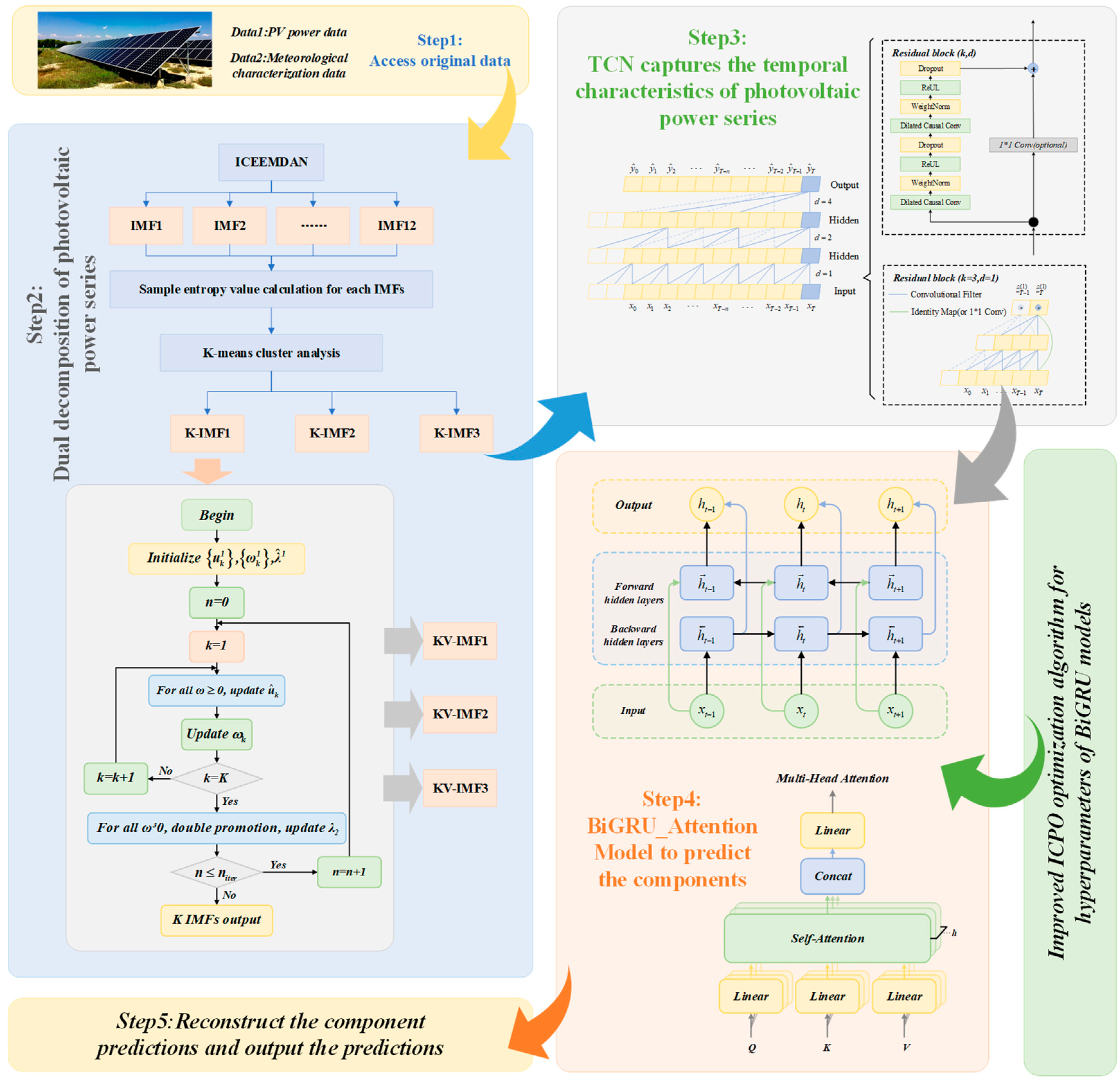
This paper introduces an integrated framework for PV power forecasting, which synergistically combines Variational Mode Decomposition (VMD) for sequence processing and an Improved CPO (ICPO) algorithm to enhance the TCN_BiGRU_Attention model’s efficacy. The role of ICPO is specifically dedicated to the hyperparameter tuning of the deep learning network, thereby refining its predictive performance. Figure 3 depicts the overall structure of this proposed system, with its operational sequence detailed in the following steps:

Step 1: Decompose the PV power sequence using VMD to obtain relatively smooth and less complex multicomponent to enhance the model’s ability to capture power generation features.

Step 2: Divide the dataset. Divide the dataset into a training set and a test set to facilitate the input model for prediction.

Step 3: Construct the TCN_BiGRU_Attention prediction model. Multiple TCN layers are used to extract the PV power series time features, BiGRU is used to capture the bi-directional information of the time series, and Attention mechanism is used to understand the importance of different time features.

Step 4: Optimize the hyperparameters of the TCN_BiGRU_Attention prediction model using the ICPO algorithm.

Step 5: The optimized TCN_BiGRU_Attention prediction model provides test samples in order to predict the PV power.

4. Case Study

4.1. Data Sources

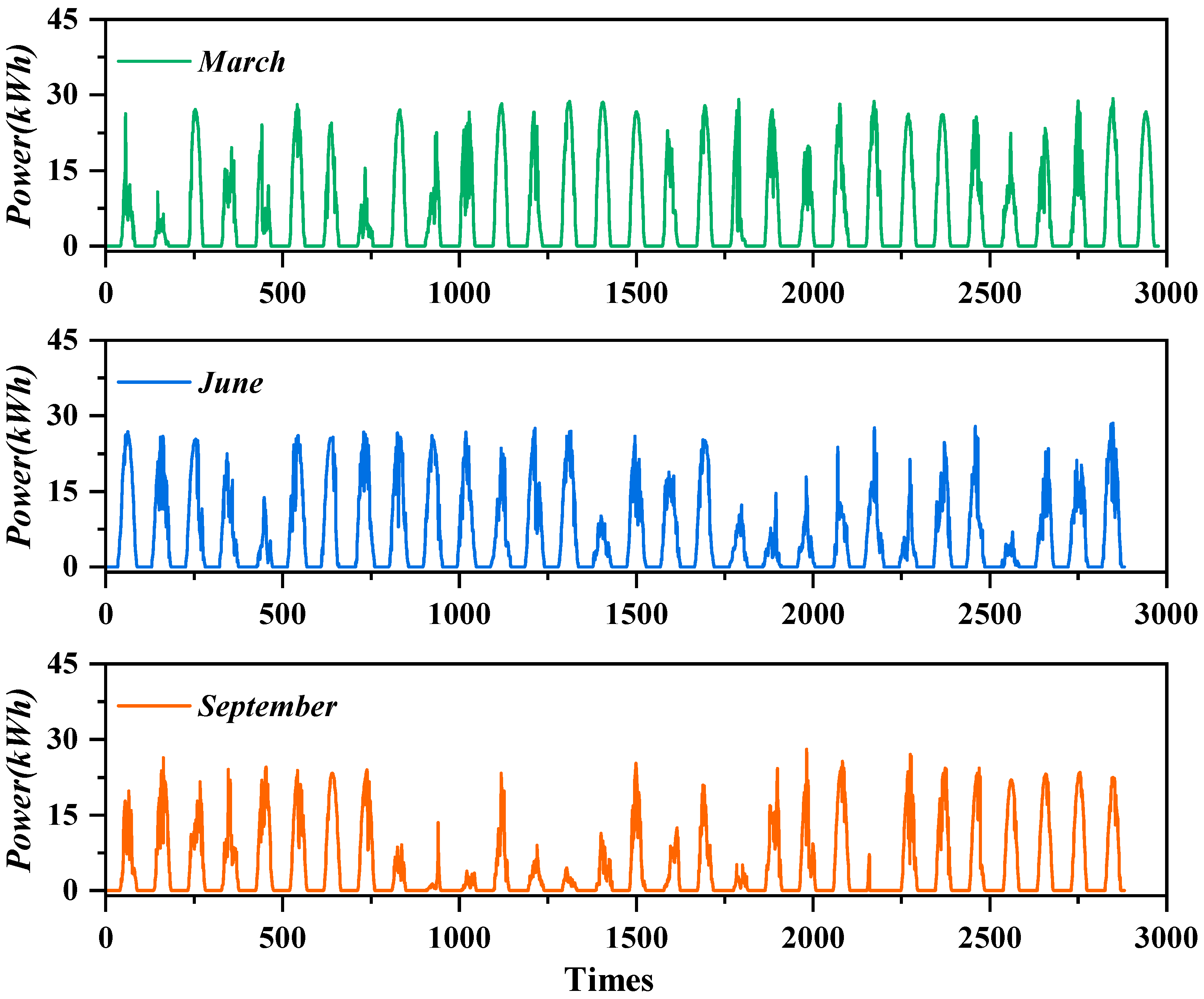
The experimental data used in this study are sourced from the Xihe Energy Meteorological Big Data Platform (https://xihe-energy.com/#climate, accessed on 1 January 2024), an integrated platform specializing in photovoltaic system monitoring that delivers remote data acquisition, intelligent alert systems, and comprehensive plant management solutions. The specific dataset originates from a northern Chinese PV power plant, comprising both historical power generation records and corresponding numerical weather prediction data provided by the China Meteorological Administration. Covering the period from 1 January to 31 December, 2021, the power generation dataset contains 35,026 recorded instances with a consistent 15-min sampling resolution. The meteorological companion dataset incorporates multiple atmospheric variables including global horizontal irradiance (W/m²), wind speed at 10 m height (m/s), precipitation rate (mm/h), ambient temperature (°C), relative humidity (%), and barometric pressure (hPa). For model development, the March 2021 power generation records were partitioned chronologically, allocating the initial 70% for training purposes and the remaining 30% for testing validation. The temporal characteristics of the original PV power measurements are illustrated in Figure 4.

4.2. Data Segmentation

This study utilizes operational data collected from a photovoltaic power plant in Northern China, complemented by meteorological forecasting datasets provided by the China Meteorological Administration (CMA). The research employs a dual-stage decomposition methodology for data preprocessing, followed by chronological partitioning of the processed sequences—designating the initial 70% of samples for model training and the remaining 30% for testing validation [37].

4.3. ICEEMDAN_VMD Secondary Decomposition

To verify the robustness and general applicability of the proposed ICEEMDAN_VMD_TCN_BiGRU_Attention forecasting framework under diverse operational conditions, this investigation implements a dual-stage decomposition strategy for processing photovoltaic power generation sequences. The methodology sequentially executes sample entropy computation after the initial ICEEMDAN decomposition, followed by systematic clustering of the resultant components through K-means analysis. The specific implementation protocol comprises the following stages:

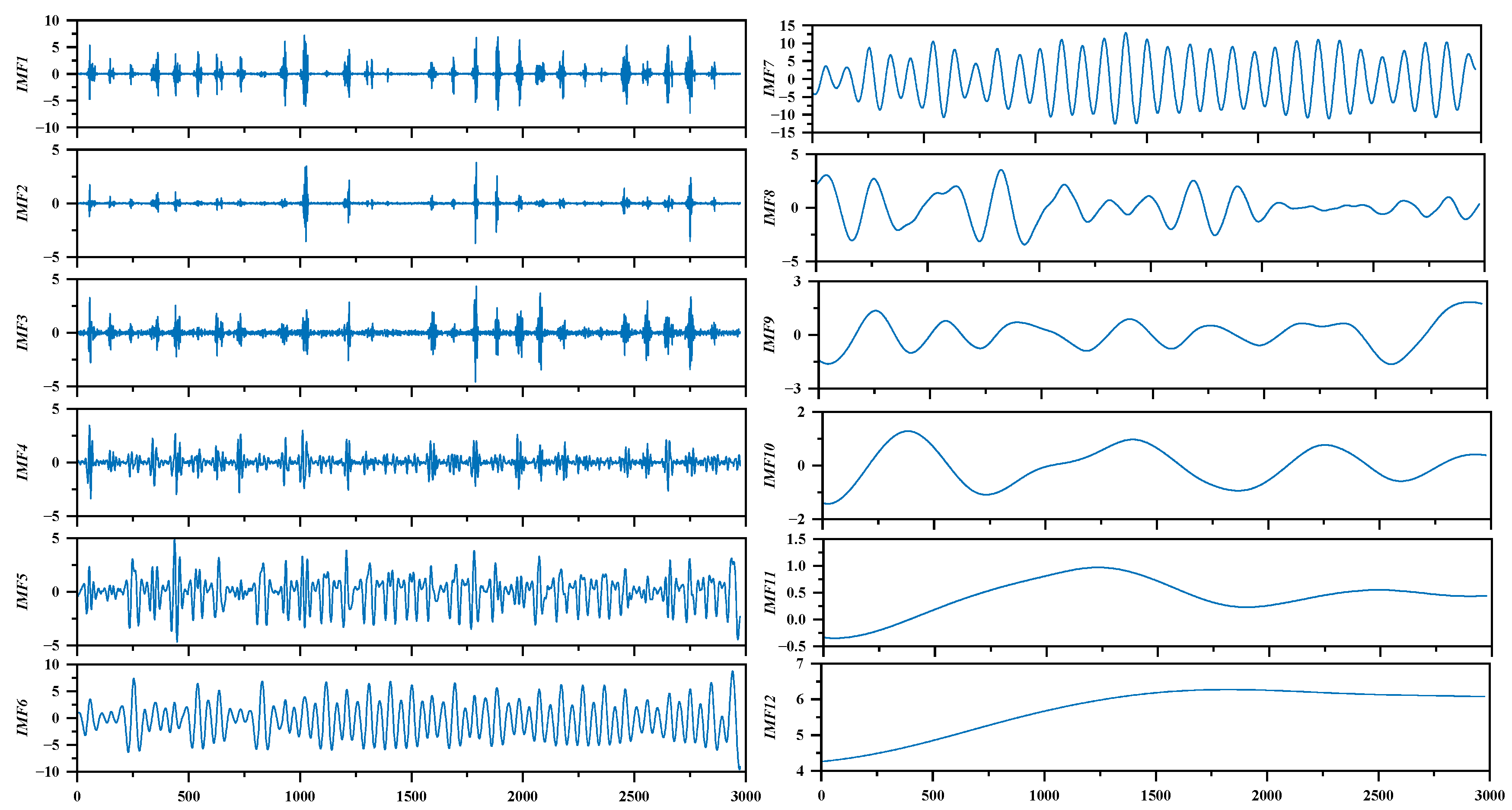
The primary decomposition phase processes raw PV power signals through the ICEEMDAN algorithm with configured parameters: ensemble size (trials) = 200 and noise standard deviation (epsilon) = 0.005, while maintaining default values for other parameters. This decomposition yields twelve Intrinsic Mode Functions (IMFs) from the input power sequences, as visually presented in Figure 5.

Subsequently, sample entropy analysis is applied to quantify the complexity of all components derived from the ICEEMDAN decomposition. Based on these entropy measurements, the K-means algorithm categorizes the decomposed elements into three separate frequency domains: high, medium, and low. The corresponding entropy values and clustering results for each component following the PV power decomposition process are systematically presented in

Table 1. Entropy calculation and K-means clustering.

Components	Sample Entropy Value	K-Means Cluster
IMF1	0.107996	1
IMF2	0.307337	3
IMF3	0.800755	2
IMF4	0.474539	2
IMF5	0.38969	3
IMF6	0.464603	2
IMF7	0.254337	3
IMF8	0.077557	1
IMF9	0.033641	1
IMF10	0.022138	1
IMF11	0.006674	1
IMF12	0.000999	1

.

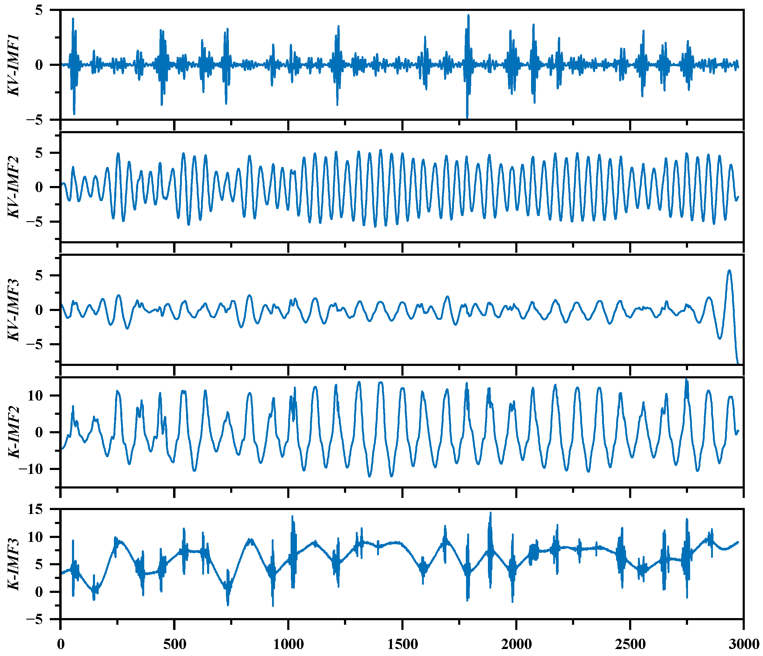
Building upon the clustering results, signal reconstruction is performed by integrating the identified high-frequency (K-IMF1), medium-frequency (K-IMF2), and low-frequency (K-IMF3) components. The high-frequency cluster subsequently undergoes refinement through Variational Mode Decomposition, generating three supplementary IMF constituents. Combined with the original medium- and low-frequency elements, this secondary processing yields a total of five distinct component series. The complete set of subsequences produced by the ICEEMDAN-VMD secondary decomposition framework is visually presented in Figure 6.

4.4. Model Performance Evaluation Metrics

A multi-faceted evaluation framework incorporating four key statistical indicators—Mean Absolute Error (MAE), Mean Squared Error (MSE), Root Mean Squared Error (RMSE), and the Coefficient of Determination (R²)—is established to systematically quantify the predictive performance of various forecasting approaches. The Mean Absolute Error (MAE) serves to measure the average absolute deviation between predicted values and actual observations. The Mean Squared Error (MSE) amplifies the influence of significant prediction errors by computing the average of squared discrepancies, while its square root, RMSE, standardizes the error magnitude to align with the original data units. The determination coefficient R² evaluates the model’s explanatory capacity by quantifying the proportion of variance in the dependent variable that is predictable from the independent variables, thereby providing a statistical measure of goodness-of-fit [38]. The mathematical formulations for these evaluation criteria are expressed as follows:

$$MAE={\displaystyle \frac{1}{N}}{\displaystyle \sum _{i=1}^N\left|Y_i-{\widehat{Y}}_i\right|}$$

(26)

$$MSE={\displaystyle \frac{1}{N}}{\displaystyle \sum _{i=1}^N{(Y_i-{\widehat{Y}}_i)}^2}$$

(27)

$$RMSE=\sqrt{{\displaystyle \frac{1}{N}}{\displaystyle \sum _{i=1}^N{(Y_i-{\widehat{Y}}_i)}^2}}$$

(28)

$$R^2=1-{\displaystyle \frac{{\displaystyle \sum _{i=1}^N{({\widehat{Y}}_i-Y_i)}^2}}{{\displaystyle \sum _{i=1}^N{({\overline{Y}}_i-Y_i)}^2}}}$$

(29)

where $N$ denotes the number of sample data points; ${\widehat{Y}}_i$ denotes the model’s predicted value for the $ith$ data point; and $Y_i$ denotes the actual value for the $ith$ data point.

5. Experimental Results and Discussion

5.1. ICPO Algorithm Performance Test

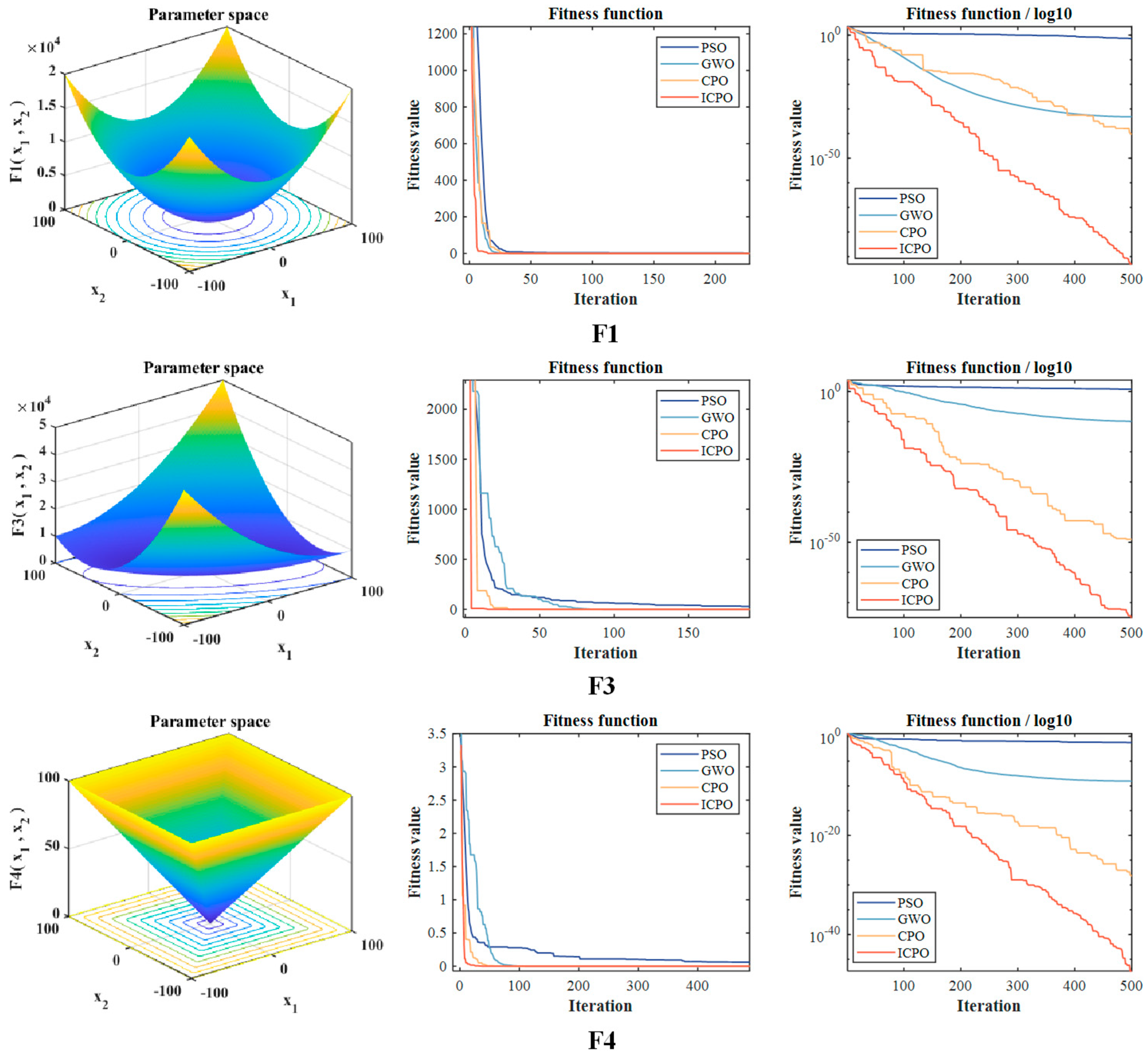
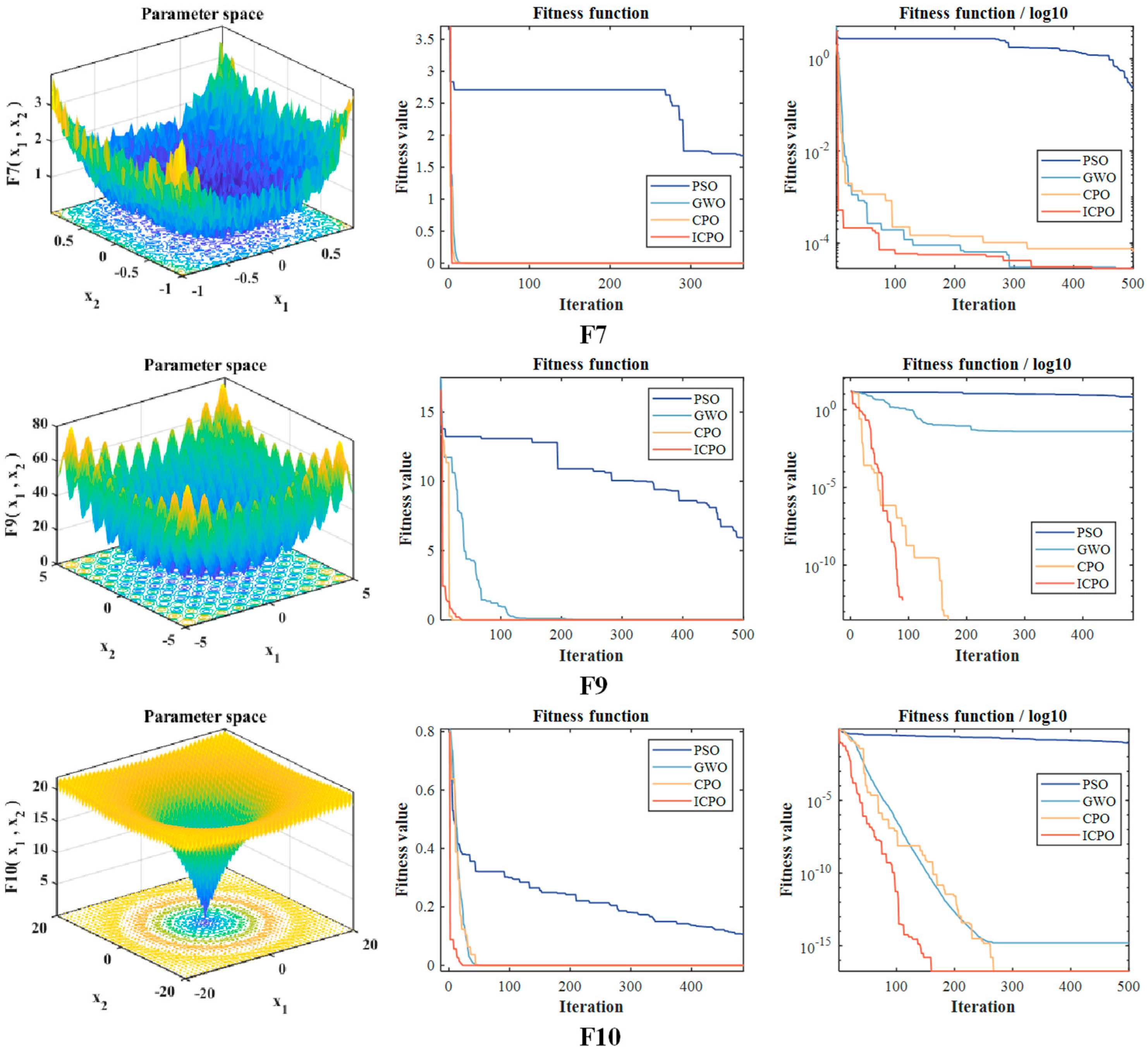
To evaluate the efficacy of the proposed ICPO algorithm, this section conducts simulation experiments utilizing six established benchmark test functions. The function set encompasses both unimodal (F1–F3) and multimodal (F4–F6) types, as detailed in

Table 2. Benchmarking functions.

Function Name	Function Formula	Dim	Range	Fmin
F1	$f_1(x)={\displaystyle \sum _{i=1}^n{x}_i^2}$	30	[−100, 100]	0
F3	$f_3(x)={\displaystyle \sum _{i=1}^n{\left({\displaystyle \sum _{j=1}^i{x}_j}\right)}^2}$	30	[−10, 10]	0
F4	$f_4(x)={\max }_i\left\{\left|x_i\right|,1\le i\le n\right\}$	30	[−100, 100]	0
F7	$f_7(x)={\displaystyle \sum _{i=1}^{n}i{x}_i^4+random\left(0,1\right)}$	30	[−1.28, 1.28]	0
F9	$f_9(x)={\displaystyle \sum _{i=1}^n\left[x_i^2-10\cos \left(2\pi x_i\right)+10\right]}$	30	[−5.12, 2.12]	0
F10	$\begin{array}{ll}{f}_{10}(x)=& -20\exp \left(-0.2\sqrt{{\displaystyle \frac{1}{n}}{\displaystyle \sum _{i=1}^n{x}_i^2}}\right)-\\ & \exp \left({\displaystyle \frac{1}{n}}{\displaystyle \sum _{i=1}^n\cos (2\pi x_i)}\right)+10+e\end{array}$	30	[−32, 32]	0

.

A comparative evaluation of the ICPO algorithm was conducted against Particle Swarm Optimization (PSO) [39], the Gray Wolf Optimizer (GWO) [40], and the standard Crested Porcupine Optimizer (CPO) using benchmark functions. For all algorithms, a population size of 50 and 500 iterations were configured, with each experiment executed over 30 independent runs. The resulting best solution, mean, and standard deviation for each technique are compiled in

Table 3. Comparison results of the algorithms.

Function Name	Optimization Algorithm	Best_Fitness	Ave	Std
F1	PSO	0.25 × 100	1.78 × 100	0.81 × 100
	GWO	3.65 × 10−35	1.93 × 10−33	2.86 × 10−33
	CPO	1.85 × 10−79	7.34 × 10−41	2.93 × 10−40
	ICPO	7.05 × 10−96	5.80 × 10−88	3.07 × 10−87
F3	PSO	6.18 × 10+01	1.30 × 10+02	3.42 × 10+01
	GWO	1.14 × 10−11	2.23 × 10−07	1.08 × 10−06
	CPO	9.16 × 10−71	1.13 × 10−40	7.66 × 10−40
	ICPO	4.16 × 10−83	1.52 × 10−72	9.88 × 10−72
F4	PSO	1.36 × 100	1.81 × 100	0.24 × 100
	GWO	2.81 × 10−09	2.34 × 10−08	2.37 × 10−08
	CPO	2.13 × 10−38	1.17 × 10−21	5.62 × 10−21
	ICPO	8.29 × 10−100	4.95 × 10−98	1.24 × 10−98
F7	PSO	2.31 × 10+00	1.44 × 10+01	1.05 × 10+01
	GWO	3.77 × 10−04	1.36 × 10−03	7.08 × 10−04
	CPO	1.19 × 10−04	1.62 × 10−03	9.79 × 10−04
	ICPO	4.35 × 10−26	2.43 × 10−24	2.04 × 10−24
F9	PSO	9.45 × 10+01	1.65 × 10+02	4.15 × 10+01
	GWO	0.00 × 100	2.50 × 100	3.96 × 100
	CPO	0.00 × 100	0.00 × 100	0.00 × 100
	ICPO	0.00 × 100	0.00 × 100	0.00 × 100
F10	PSO	1.16 × 100	2.32 × 100	4.40 × 10−01
	GWO	3.59 × 10−14	4.32 × 10−14	5.29 × 10−15
	CPO	4.44 × 10−120	6.57 × 10−126	8.52 × 10−126
	ICPO	0.00 × 100	0.00 × 100	0.00 × 100

.

As evidenced by the comparative data in Table 3, the proposed ICPO algorithm consistently yields lower mean values and standard deviations across unimodal benchmark functions (F1, F3, F4) when evaluated against PSO, GWO, and standard CPO implementations. These statistical outcomes confirm both the superior stability of ICPO’s optimization process and its enhanced solution quality relative to the competing algorithms. Furthermore, the method demonstrates comparable robustness when applied to multimodal test functions. To enable more intuitive assessment of algorithmic convergence characteristics, we present both original and logarithmically scaled convergence plots for all six benchmark functions, accounting for the distinct optimization behaviors observed across different methods. Figure 7 illustrates the convergence patterns for unimodal functions, while Figure 8 displays the corresponding trajectories for multimodal optimization problems.

Analysis of the convergence characteristics presented in Figure 7 and Figure 8 indicates that the ICPO approach achieves faster convergence rates on both unimodal (F1–F3) and multimodal test functions when compared to PSO, GWO, and the standard CPO. Furthermore, the algorithm demonstrates notable efficiency in locating promising solution regions and rapidly converging toward optimal solutions, consequently reducing the computational time required for optimization. These consistent results across diverse function types validate the algorithm’s strengthened global search capability compared to other competing techniques.

5.2. Comparison of Forecast Results for March

A variety of forecasting methodologies have been developed for photovoltaic power prediction in prior research. To ensure a comprehensive and impartial evaluation of our proposed framework, this study implements a component-wise prediction strategy: each decomposed subsequence is forecasted independently, followed by a weighted aggregation of all component predictions to generate the final photovoltaic power output. For systematic comparison, we constructed nine distinct model configurations. For clarity in subsequent discussion, these comparative models are designated as Model 1 through Model 9, with detailed specifications provided in

Table 4. Code name of each model.

Name	Models
Model 1	BP
Model 2	BiGRU
Model 3	TCN_BiGRU
Model 4	VMD_TCN_BiGRU
Model 5	ICEEMDAN_VMD_BiGRU
Model 6	ICEEMDAN_VMD_TCN_BiGRU
Model 7	ICEEMDAN_VMD_TCN_BiGRU_Attention
Model 8	ICEEMDAN_VMD_CPO_TCN_BiGRU_Attention
Model 9	ICEEMDAN_VMD_ICPO_TCN_BiGRU_Attention

.

In order to further compare the performance of each comparison model, the evaluation index situation of each model is given as shown in

Table 5. Comparison of PV power prediction results for the March dataset.

	MSE	RMSE	MAE	R2
Model 1	3.4083	1.8462	1.0015	95.8351
Model 2	2.2969	1.5156	0.9296	96.8496
Model 3	1.9939	1.4120	0.8589	97.5324
Model 4	1.5139	1.2304	0.8745	97.8901
Model 5	0.9043	0.9509	0.6943	98.9897
Model 6	0.7570	0.8701	0.5985	99.0506
Model 7	0.6663	0.8163	0.4702	99.2089
Model 8	0.4697	0.6853	0.3843	99.4391
Model 9	0.3456	0.5879	0.3396	99.5910

.

A systematic examination of the comparative results presented in Table 4 and Figure 7 yields the following analytical insights: (a) Beginning with the baseline models, the BiGRU demonstrates a clear advantage over the conventional BP network, MSE with a reduction to 2.2969 and R² improves to 96.85%. This result aligns with existing literature on the strength of recurrent architectures in modeling temporal dependencies in sequential data, such as PV power generation. (b) The integration of TCN_BiGRU further improves predictive accuracy. The TCN architecture employs dilated convolutions to capture multi-scale temporal features, effectively complementing the BiGRU sequential processing capabilities. This is reflected in a decreased MSE of 1.9939 and an increased R² of 97.53%. (c) The introduction of Variational Mode Decomposition (VMD_TCN_BiGRU) yields notable improvement, with MSE declining to 1.5139 and RMSE to 1.2304. This suggests that VMD contributes to noise reduction and signal stabilization, thereby facilitating more robust feature extraction. (d) A dual decomposition strategy incorporating ICEEMDAN followed by VMD constitutes a significant advancement. Model 6, in particular, achieves an MSE of 0.7570, underscoring the efficacy of hierarchical decomposition in isolating interpretable modes and mitigating non-stationarity. (e) ICEEMDAN_VMD_TCN_BiGRU_Attention further enhances performance, yielding an MSE of 0.6663 and an R² of 99.21%. This aligns with established findings that attention improves interpretability and long-range dependency modeling. (f) The application of hyperparameter optimization via the CPO algorithm results in consistent gains (MSE = 0.4697). The most substantial improvement, however, is achieved by the proposed Improved CPO, which attains an MSE of 0.3456 and R² of 99.59%. This underscores the efficiency of chaotic mapping and Lévy flight strategies in enhancing optimization robustness and avoiding premature convergence.

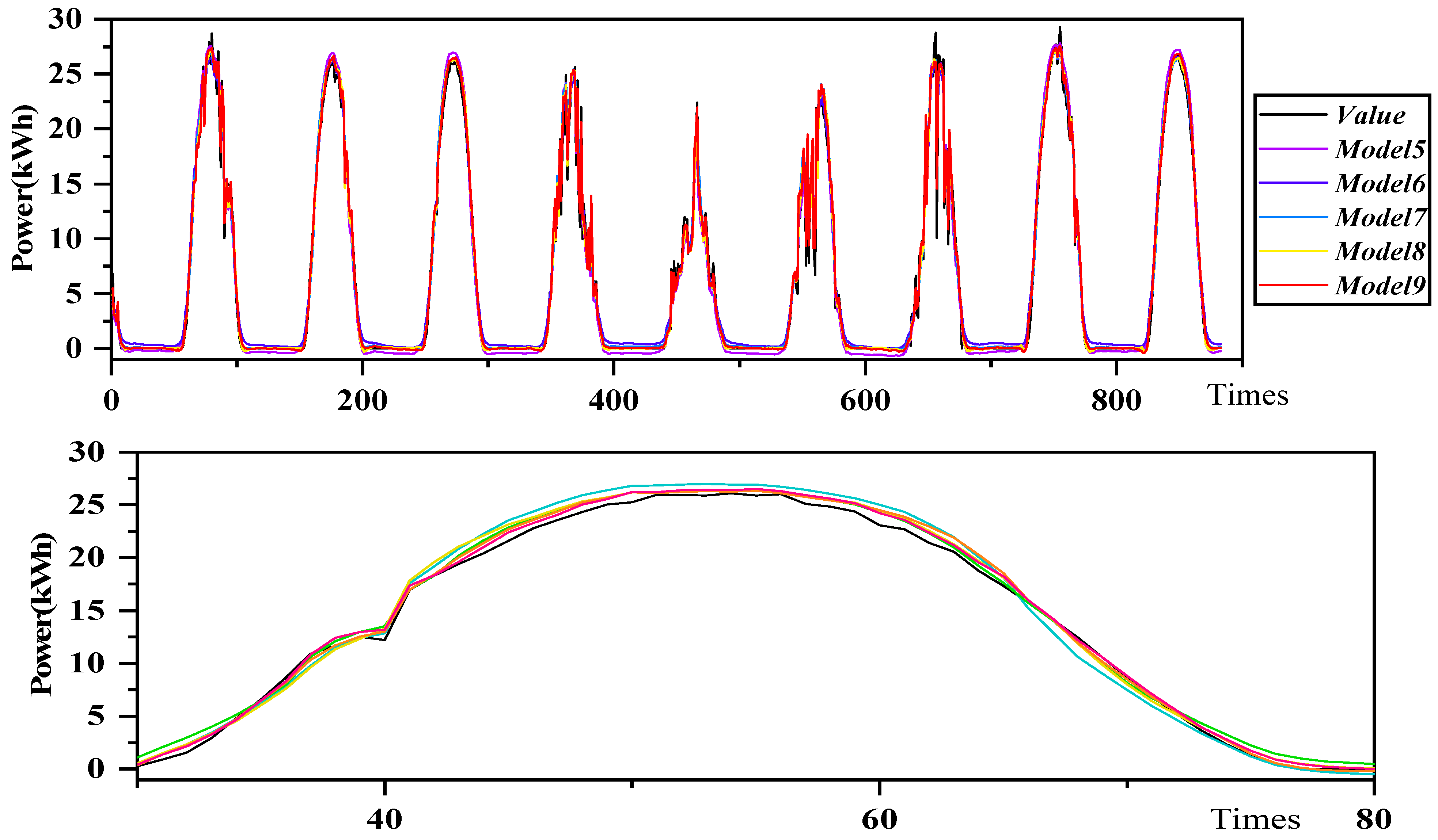
As visually summarized in Figure 9, prediction fidelity improves progressively across model variants. The proposed Model 9 exhibits a high degree of alignment with the actual power curve, including during periods of rapid fluctuation, whereas baseline models (e.g., Models 1 and 2) display noticeable deviations. These observations corroborate the quantitative findings and affirm the robustness of the optimized hybrid framework.

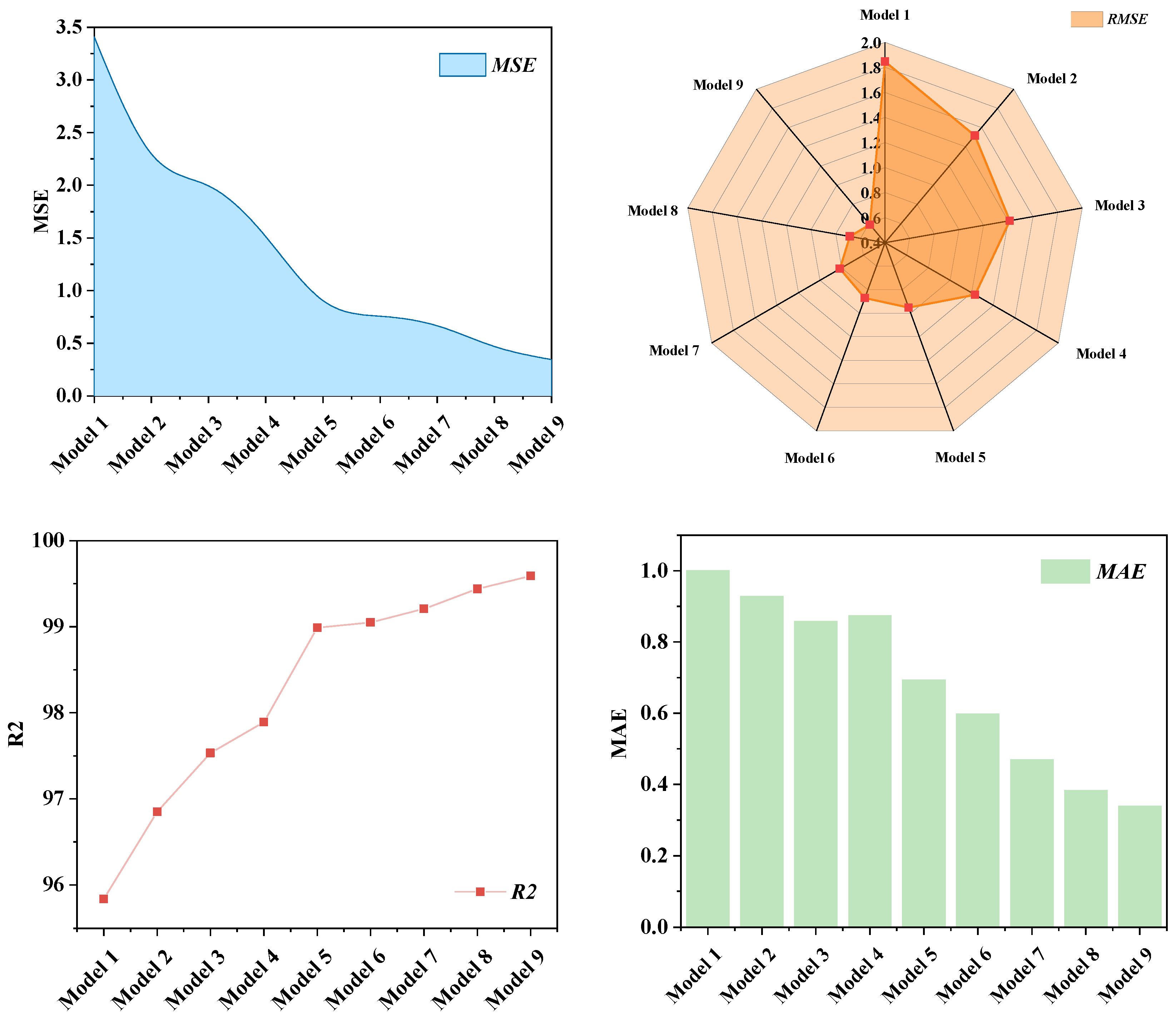
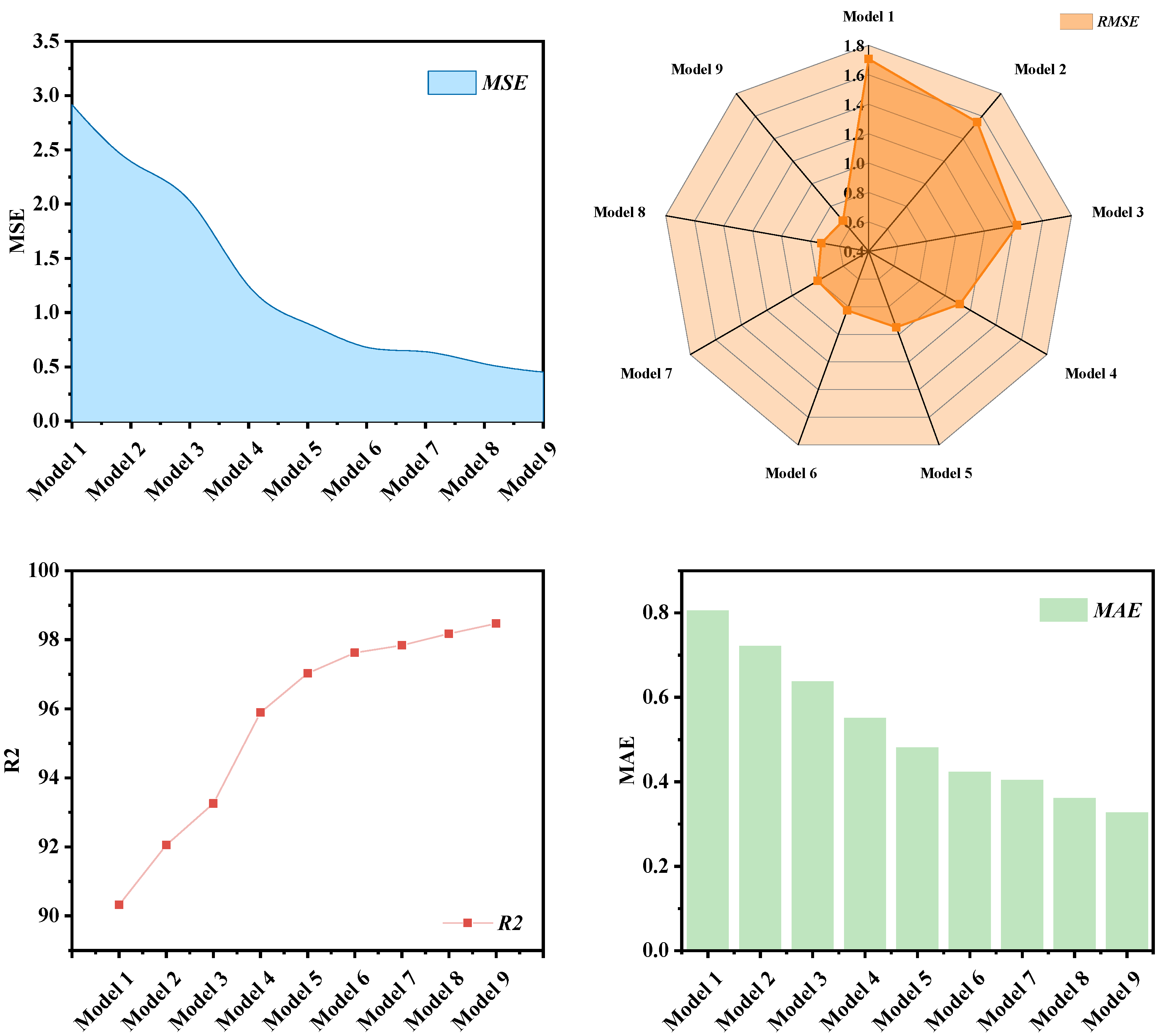
In order to visualize the best prediction effect of the combined model proposed in this paper, this paper also analyzes the prediction results of each model with normal distribution, and it can be seen through Figure 10 that the model proposed in this paper is more skewed towards 0, which indicates the best prediction performance of the hybrid learning model. In order to visualize the performance evaluation results of the combined models, this paper also plots the performance indicators of the prediction results of the combined models on the March dataset in radar charts, dot line charts, bar charts and spline charts, just to show the prediction effect of each combined model more intuitively, and it can be seen very intuitively in Figure 10, the combined prediction model proposed in this paper has very good prediction of the PV power dataset of the month of March.

5.3. Comparison of Forecast Results for May and June

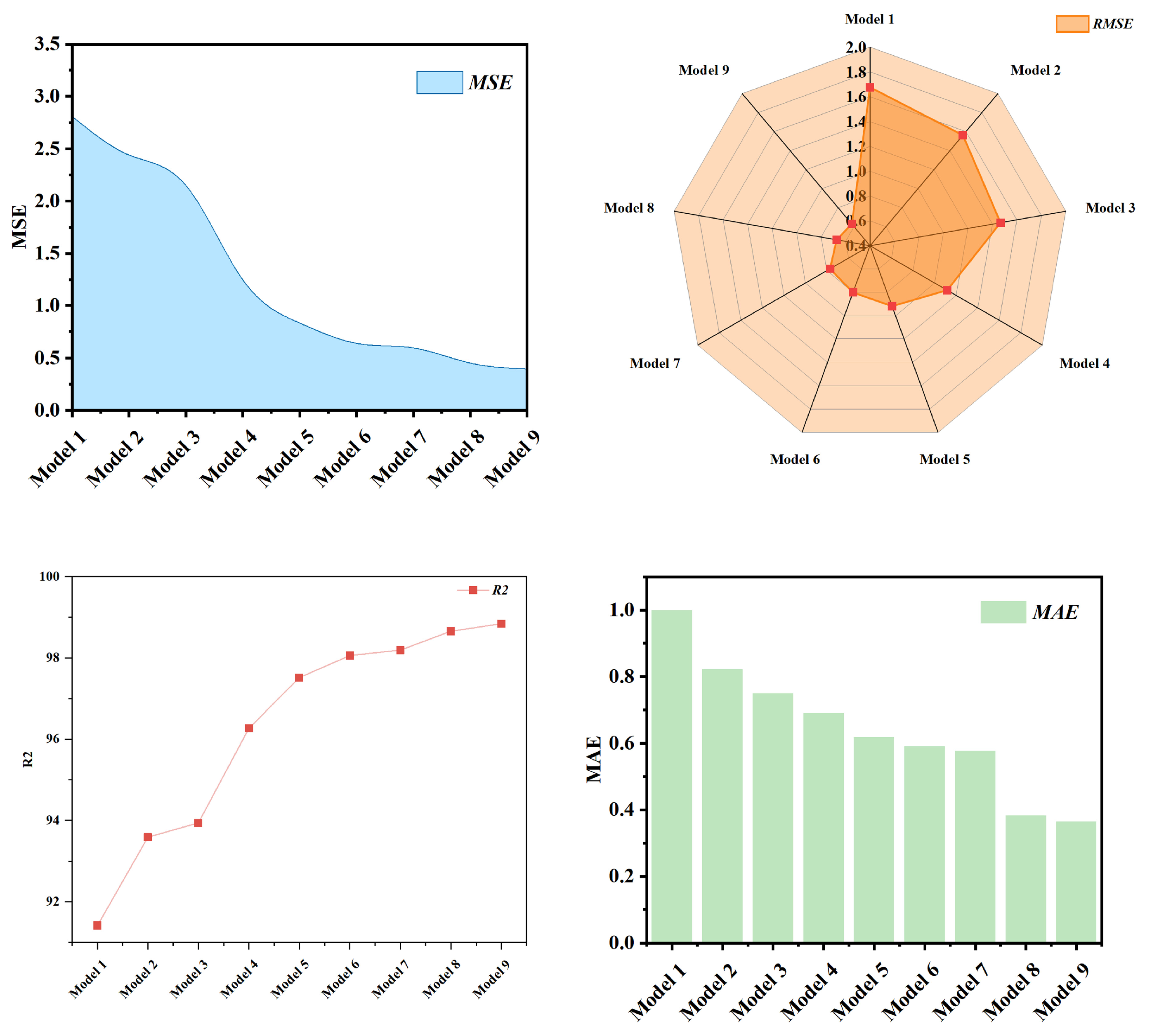
The generalizability and robustness of the proposed hybrid model were further assessed on additional PV power datasets from January and July. This evaluation aims to verify its stable predictive accuracy and generalization capability beyond the initial training data. The performance metrics for these temporal frames are detailed in

Table 6. Comparison of PV power prediction results for the January dataset.

	MSE	RMSE	MAE	R2
Model 1	2.9165	1.7078	0.8060	90.3189
Model 2	2.3931	1.5470	0.7216	92.0551
Model 3	2.0298	1.4247	0.6385	93.2585
Model 4	1.2456	1.1161	0.5518	95.8898
Model 5	0.8989	0.9481	0.6408	97.0303
Model 6	0.6822	0.8259	0.4237	97.6232
Model 7	0.6390	0.7994	0.4041	97.8418
Model 8	0.5280	0.7266	0.3612	98.1759
Model 9	0.4519	0.6722	0.3275	98.4679

(January) and

Table 7. Comparison of PV power prediction results for the July dataset.

	MSE	RMSE	MAE	R2
Model 1	2.8096	1.6762	0.9986	91.4154
Model 2	2.4406	1.5622	0.8213	93.5919
Model 3	2.1500	1.4663	0.7488	93.9420
Model 4	1.2473	1.1168	0.9500	0.9627
Model 5	0.8345	0.9184	0.6177	97.5177
Model 6	0.6400	0.8003	0.5896	98.0590
Model 7	0.5956	0.7718	0.5768	98.1930
Model 8	0.4525	0.6727	0.3828	98.6588
Model 9	0.3951	0.6286	0.3650	98.8414

(July).

Table 6 and Table 7 show the prediction results of the various combinations of models on the January and July datasets, respectively. The performance of each model was evaluated using four metrics: MSE, RMSE, MAE, and R².

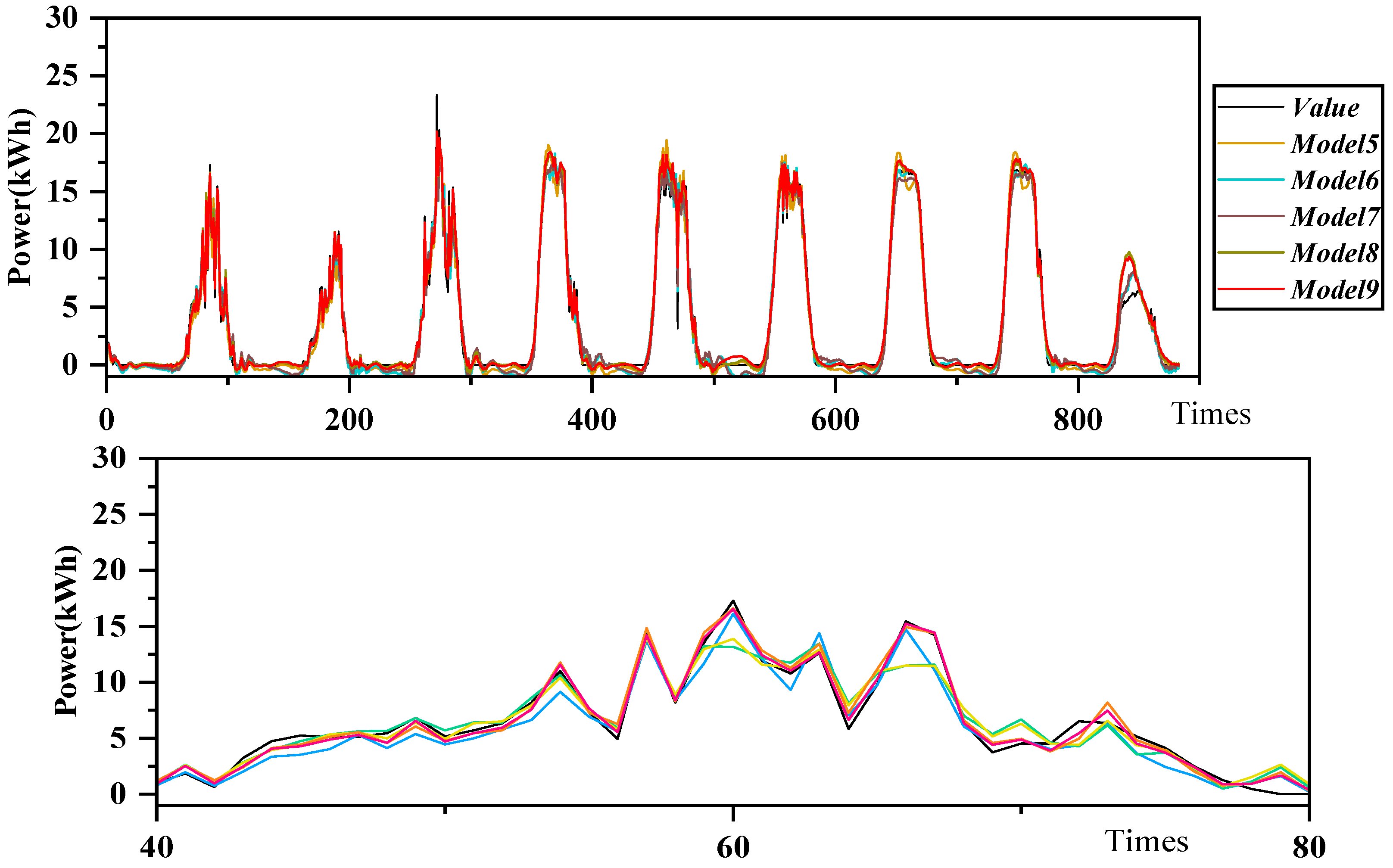
From Table 6, we can observe the following trends: (a) Among all the metrics, the combined model proposed in this paper has the best performance, with an MSE of 0.4519, an RMSE of 0.6722, an MAE of 0.3275, and an R² of 98.47%. (b) From the simple BiGRU model to the more complex ICEEMDAN_VMD_ICPO _TCN_BiGRU _Attention model, the performance of the model increases sequentially. This indicates that the dual decomposition strategy combined with the hybrid learning model proposed in this study helps to improve the prediction accuracy of PV power pairs. Table 7 shows the following trends: (a) Similar to the January dataset, the ICEEMDAN_VMD_ICPO _TCN_BiGRU_Attention model achieves the best performance on the July dataset with the lowest MSE (0.3951), RMSE (0.6286), MAE (0.3650), and R² (98.84%). (b) The ICEEMDAN_VMD_ICPO _TCN_BiGRU_Attention model is the best predictor of PV power pairs in terms of performance, and it is also the best predictor of PV power pairs in terms of performance. The performance improvement from the BiGRU model to the ICEEMDAN_VMD_ICPO _TCN_BiGRU_Attention model is consistent in both datasets, which confirms the effectiveness of the proposed combined model. All models in the July dataset show higher errors compared to the January dataset, attributed to the differences in data features and the complexity of the underlying patterns. In summary, the combined models combining TCN, BiGRU, attention mechanism and dual decomposition strategy ICEEMDAN_VMD all outperform the individual models on the PV power dataset. The ICEEMDAN_VMD_ICPO _TCN_BiGRU_Attention model has the best overall performance, highlighting the advantages of feature fusion and temporal aggregation in the time series prediction task. To visualize the prediction results, Figure 11 shows the combined model prediction fit curve for the January generation power dataset, Figure 12 shows the Plot of the results of the predictive performance assessment of the integrated model for the January dataset. Figure 13 shows the combined model prediction fit curve for the July power generation dataset, Figure 14 shows the Plot of the results of the predictive performance assessment of the integrated model for the July dataset.

Figure 11 and Figure 13 show the prediction fitting curves of the nine combined models for the January and July datasets. The fitting curves of the combined prediction models show obvious superiority in terms of high fitting accuracy and robustness, indicating that the hybrid learning model used in this paper has certain prediction accuracy and reliability for the PV power prediction strategy. Figure 12 and Figure 14 show the performance evaluation of the January and July datasets on the hybrid learning model proposed in this paper.

6. Conclusions

In this paper, a hybrid learning model based on dual decomposition model and optimized decomposition model is proposed in order to consider one decomposition of PV power using ICEEMDAN, and then using K-means cluster analysis to cluster and analyze the decomposed components into three components of high frequency, mid-frequency, and low-frequency, and then using VMD to decompose the high-frequency component, and finally inputting the decomposed component plus the feature data into the TCN_BiGRU_Attention prediction model for prediction. In order to improve the estimation accuracy of the TCN_BiGRU_Attention model, ICPO is used to optimize the hyperparameters of the TCN_BiGRU_Attention model. This study takes the data of a photovoltaic power station in northern China in March as an example and uses the data of January and July in this region to test the generalization ability. The results are discussed as follows.

(a) The ICEEMDAN algorithm is employed to decompose the original dataset and extract feature signals across various frequency bands. Subsequently, K-means clustering is utilized to segment these decomposed feature signals into several subsequences, thereby delving deeper into the underlying structure of the data. In the final step, VMD is applied to further decompose each subsequence, thereby extracting more refined feature details.

(b) In this paper, the standard CPO algorithm is optimized and the ICPO method is introduced to optimize the hyperparameters of the TCN_BiGRU_Attention model. It reduces the number of manual adjustments to the parameters of the TCN_BiGRU_Attention model and shortens the computation time.

(c) Hybrid learning models have better prediction accuracy than single prediction models. Each PV power sequence has different features and attributes, which makes it difficult for a single prediction model BiGRU to predict various types of sequences. The MSE, RMSE, MAE and R² of the hybrid learning model are 0.3456, 0.5879, 0.3396, and 99.59%, respectively, which is an improvement of 3.0627, 1.2583, 0.6619, and 3.876% compared to the single model.

The developed hybrid learning paradigm demonstrates robust PV power forecasting capabilities through three interconnected methodological dimensions: advanced data preprocessing, systematic hyperparameter optimization, and sophisticated predictive model architecture. Experiments verify the stability and reliability of the model.

References

1. Antonanzas, J.; Osorio, N.; Escobar, R.; Urraca, R.; Martinez-De-Pison, F.J.; Antonanzas-Torres, F. Review of photovoltaic power forecasting. Sol. Energy 2016, 136, 78–111. [Google Scholar] [CrossRef]
2. Das, U.K.; Tey, K.S.; Seyedmahmoudian, M.; Mekhilef, S.; Idris, M.Y.I.; Van Deventer, W.; Horan, B.; Stojcevski, A. Forecasting of photovoltaic power generation and model optimization: A review. Renew. Sustain. Energy Rev. 2018, 81, 912–928. [Google Scholar] [CrossRef]
3. Wang, K.; Qi, X.; Liu, H. Photovoltaic power forecasting based LSTM-Convolutional Network. Energy 2019, 189, 116225. [Google Scholar] [CrossRef]
4. Mayer, M.J.; Gróf, G. Extensive comparison of physical models for photovoltaic power forecasting. Appl. Energy 2021, 283, 116239. [Google Scholar] [CrossRef]
5. Mellit, A.; Pavan, A.M.; Lughi, V. Deep learning neural networks for short-term photovoltaic power forecasting. Renew. Energy 2021, 172, 276–288. [Google Scholar] [CrossRef]
6. Li, P.; Zhou, K.; Lu, X.; Yang, S. A hybrid deep learning model for short-term PV power forecasting. Appl. Energy 2020, 259, 114216. [Google Scholar] [CrossRef]
7. van Heerden, L.; Vermeulen, H.J.; van Staden, C. Wind power forecasting using hybrid recurrent neural networks with empirical mode decomposition. In Proceedings of the 2022 IEEE International Conference on Environment and Electrical Engineering and 2022 IEEE Industrial and Commercial Power Systems Europe (EEEIC/I&CPS Europe), Prague, Czech Republic, 28 June–1 July 2022; IEEE: New York, NY, USA, 2022; pp. 1–6. [Google Scholar]
8. Fara, L.; Diaconu, A.; Craciunescu, D.; Fara, S. Forecasting of energy production for photovoltaic systems based on ARIMA and ANN advanced models. Int. J. Photoenergy 2021, 2021, 6777488. [Google Scholar] [CrossRef]
9. Wan, C.; Zhao, J.; Song, Y.; Xu, Z.; Lin, J.; Hu, Z. Photovoltaic and solar power forecasting for smart grid energy management. CSEE J. Power Energy Syst. 2015, 1, 38–46. [Google Scholar] [CrossRef]
10. Pan, M.; Li, C.; Gao, R.; Huang, Y.; You, H.; Gu, T.; Qin, F. Photovoltaic power forecasting based on a support vector machine with improved ant colony optimization. J. Clean. Prod. 2020, 277, 123948. [Google Scholar] [CrossRef]
11. Mayer, M.J. Benefits of physical and machine learning hybridization for photovoltaic power forecasting. Renew. Sustain. Energy Rev. 2022, 168, 112772. [Google Scholar] [CrossRef]
12. Scott, C.; Ahsan, M.; Albarbar, A. Machine learning for forecasting a photovoltaic (PV) generation system. Energy 2023, 278, 127807. [Google Scholar] [CrossRef]
13. Lateko, A.A.H.; Yang, H.T.; Huang, C.M. Short-term PV power forecasting using a regression-based ensemble method. Energies 2022, 15, 4171. [Google Scholar] [CrossRef]
14. Zhou, B.; Chen, X.; Li, G.; Gu, P.; Huang, J.; Yang, B. Xgboost–sfs and double nested stacking ensemble model for photovoltaic power forecasting under variable weather conditions. Sustainability 2023, 15, 13146. [Google Scholar] [CrossRef]
15. Liao, S.; Tian, X.; Liu, B.; Liu, T.; Su, H.; Zhou, B. Short-term wind power prediction based on LightGBM and meteorological reanalysis. Energies 2022, 15, 6287. [Google Scholar] [CrossRef]
16. Rana, M.; Rahman, A. Multiple steps ahead solar photovoltaic power forecasting based on univariate machine learning models and data re-sampling. Sustain. Energy Grids Netw. 2020, 21, 100286. [Google Scholar] [CrossRef]
17. Markovics, D.; Mayer, M.J. Comparison of machine learning methods for photovoltaic power forecasting based on numerical weather prediction. Renew. Sustain. Energy Rev. 2022, 161, 112364. [Google Scholar] [CrossRef]
18. Huang, C.J.; Kuo, P.H. Multiple-input deep convolutional neural network model for short-term photovoltaic power forecasting. IEEE Access 2019, 7, 74822–74834. [Google Scholar] [CrossRef]
19. Li, G.; Xie, S.; Wang, B.; Xin, J.; Li, Y.; Du, S. Photovoltaic power forecasting with a hybrid deep learning approach. IEEE Access 2020, 8, 175871–175880. [Google Scholar] [CrossRef]
20. Wang, K.; Qi, X.; Liu, H. A comparison of day-ahead photovoltaic power forecasting models based on deep learning neural network. Appl. Energy 2019, 251, 113315. [Google Scholar] [CrossRef]
21. Huang, C.; Yang, M. Memory long and short term time series network for ultra-short-term photovoltaic power forecasting. Energy 2023, 279, 127961. [Google Scholar] [CrossRef]
22. Liu, H.; Gao, Q.; Ma, P. Photovoltaic generation power prediction research based on high quality context ontology and gated recurrent neural network. Sustain. Energy Technol. Assess. 2021, 45, 101191. [Google Scholar] [CrossRef]
23. Farah, S.; Humaira, N.; Aneela, Z.; Steffen, E. Short-term multi-hour ahead country-wide wind power prediction for Germany using gated recurrent unit deep learning. Renew. Sustain. Energy Rev. 2022, 167, 112700. [Google Scholar] [CrossRef]
24. Wang, L.; Liu, Y.; Li, T.; Xie, X.; Chang, C. Short-term PV power prediction based on optimized VMD and LSTM. IEEE Access 2020, 8, 165849–165862. [Google Scholar] [CrossRef]
25. Simeunović, J.; Schubnel, B.; Alet, P.J.; Carrillo, R.E. Spatio-temporal graph neural networks for multi-site PV power forecasting. IEEE Trans. Sustain. Energy 2021, 13, 1210–1220. [Google Scholar] [CrossRef]
26. Zhang, C.; Peng, T.; Nazir, M.S. A novel integrated photovoltaic power forecasting model based on variational mode decomposition and CNN-BiGRU considering meteorological variables. Electr. Power Syst. Res. 2022, 213, 108796. [Google Scholar] [CrossRef]
27. Thanh, P.N.; Cho, M.Y.; Chang, C.L.; Chen, M.-J. Short-term three-phase load prediction with advanced metering infrastructure data in smart solar microgrid based convolution neural network bidirectional gated recurrent unit. IEEE Access 2022, 10, 68686–68699. [Google Scholar] [CrossRef]
28. Zhou, H.; Wang, J.; Ouyang, F.; Cui, C.; Li, X. A two-stage method for ultra-short-term pv power forecasting based on data-driven. IEEE Access 2023, 11, 41175–41189. [Google Scholar] [CrossRef]
29. Zhang, F.; Guo, J.; Yuan, F.; Shi, Y.; Li, Z. Research on denoising method for hydroelectric unit vibration signal based on ICEEMDAN–PE–SVD. Sensors 2023, 23, 6368. [Google Scholar] [CrossRef]
30. Kaytez, F. A hybrid approach based on autoregressive integrated moving average and least-square support vector machine for long-term forecasting of net electricity consumption. Energy 2020, 197, 117200. [Google Scholar] [CrossRef]
31. Sleiman, A.; Su, W. Combined K-means clustering with neural networks methods for PV short-term generation load forecasting in electric utilities. Energies 2024, 17, 1433. [Google Scholar] [CrossRef]
32. Zhou, D.; Wang, B. Battery health prognosis using improved temporal convolutional network modeling. J. Energy Storage 2022, 51, 104480. [Google Scholar] [CrossRef]
33. Liu, J.; Lei, X.; Zhang, Y.; Pan, Y. The prediction of molecular toxicity based on BiGRU and GraphSAGE. Comput. Biol. Med. 2023, 153, 106524. [Google Scholar] [CrossRef]
34. Aznaran, F.R.A.; Farrell, P.E.; Kirby, R.C. Transformations for Piola-mapped elements. SMAI J. Comput. Math. 2022, 8, 399–437. [Google Scholar] [CrossRef]
35. Abdel-Basset, M.; Mohamed, R.; Abouhawwash, M. Crested Porcupine Optimizer: A new nature-inspired metaheuristic. Knowl.-Based Syst. 2024, 284, 111257. [Google Scholar] [CrossRef]
36. Zhang, C.; Zhou, J.; Li, C.; Fu, W.; Peng, T. A compound structure of ELM based on feature selection and parameter optimization using hybrid backtracking search algorithm for wind speed forecasting. Energy Convers. Manag. 2017, 143, 360–376. [Google Scholar] [CrossRef]
37. Haben, S.; Arora, S.; Giasemidis, G.; Voss, M.; Greetham, D.V. Review of low voltage load forecasting: Methods, applications, and recommendations. Appl. Energy 2021, 304, 117798. [Google Scholar] [CrossRef]
38. Jahromi, A.J.; Mohammadi, M.; Afrasiabi, S.; Afrasiabi, M.; Aghaei, J. Probability density function forecasting of residential electric vehicles charging profile. Appl. Energy 2022, 323, 119616. [Google Scholar] [CrossRef]
39. Morel, G.; Grabot, B. Engineering Applications of Artificial Intelligence; IMS: Virginia Beach, VA, USA, 2003; p. 16. [Google Scholar]
40. Zhang, Y.; Wang, Y.; Zhang, C.; Qiao, X.; Ge, Y.; Li, X.; Peng, T.; Nazir, M.S. State-of-health estimation for lithium-ion battery via an evolutionary Stacking ensemble learning paradigm of random vector functional link and active-state-tracking long–short-term memory neural network. Appl. Energy 2024, 356, 122417. [Google Scholar] [CrossRef]
Figure 1. The model framework of the TCN.
Energies 18 06159 g001
Figure 2. The structure of the multi-head self-attention mechanism.
Energies 18 06159 g002
Figure 3. Framework of the proposed model.
Energies 18 06159 g003
Figure 4. Raw PV output power data plot.
Energies 18 06159 g004
Figure 5. Subsequences obtained from ICEEMDAN decomposition.
Energies 18 06159 g005
Figure 6. ICEEMDAN_VMD Photovoltaic Output Power Data Secondary Decomposition Components.
Energies 18 06159 g006
Figure 7. Convergence curve of unimodal test functions.
Energies 18 06159 g007
Figure 8. Convergence curve of multimodal test functions.
Energies 18 06159 g008
Figure 9. Prediction results for all models for the March dataset.
Energies 18 06159 g009
Figure 10. Plot of the results of the predictive performance assessment of the integrated model for the March dataset.
Energies 18 06159 g010
Figure 11. Prediction results for all models for the January dataset.
Energies 18 06159 g011
Figure 12. Plot of the results of the predictive performance assessment of the integrated model for the January dataset.
Energies 18 06159 g012
Figure 13. Prediction results for all models for the July dataset.
Energies 18 06159 g013
Figure 14. Plot of the results of the predictive performance assessment of the integrated model for the July dataset.
Energies 18 06159 g014