Bearing Fault Diagnosis Using Torque Observer in Induction Motor

Abstract

This study introduces a sensorless fault diagnosis method for efficiently detecting bearing faults in induction motors. The proposed method eliminates the need for torque sensors, frequency sensors, thermal cameras, or real-time Fast Fourier Transform (FFT) tools. Induction motors are commonly utilized in a variety of industrial applications, including fans, pumps, and home appliances, due to their straightforward construction, affordability, and robust reliability. Traditional bearing fault diagnosis methods often rely on additional hardware such as vibration or thermal sensors. Additionally, approaches employing Artificial Intelligence (AI) and real-time FFT processing require advanced and expensive hardware capabilities. However, many V/f control systems are primarily intended for cost-effective and simple implementations, making resource-intensive approaches undesirable. Therefore, such methods present limitations for these use cases. To address these challenges, this paper presents a sensorless detection technique that estimates torque via a flux observer, removing the dependence on external sensors. The estimated torque is processed using an offline FFT to identify amplitude changes within bearing fault frequency bands. Here, the FFT-based frequency analysis is performed offline and is used to design a targeted band-pass filter (BPF). The torque signal, after passing through the BPF, undergoes a straightforward threshold-based logic to assess the existence of faults. Compared to AI- or data-driven approaches, the proposed method provides a lightweight, interpretable, and sensorless solution without the need for additional training or high-end processors. Despite its straightforward approach, the technique achieves effective detection of bearing faults across various components and speeds, making it ideal for embedded and economically constrained motor applications.

1. Introduction

Induction motors are widely employed in systems such as household appliances, pumps, railway applications, and electric vehicles, owing to their uncomplicated construction, low cost, and high reliability. Nevertheless, faults in these motors can result in performance loss or critical operational failures, particularly in high-power environments. As reported by IEEE, about 42% of induction motor failures are attributed to bearing faults, with stator faults at 28%, rotor faults at 8%, and other causes accounting for 22% [1]. Since bearings support the rotating components and are subjected to diverse mechanical and thermal stresses, proactive detection of bearing faults is essential for maintaining motor reliability.

To detect such faults, a range of diagnostic techniques has been developed. Thermal imaging methods combined with signal processing, such as two-dimensional discrete wavelet transform (2D-DWT) [2] or convolutional neural networks (CNNs) [3], provide real-time and non-contact monitoring capabilities. However, these techniques necessitate the use of costly thermal cameras, and their performance is susceptible to environmental factors such as ambient temperature and humidity.

Vibration-based approaches are extensively utilized as well. Fault detection models using externally induced vibration are presented in [4], while foundational vibration signal processing techniques were introduced in [5]. Frequency-domain analysis through FFT or time–frequency analysis has been employed in [6,7] to identify frequencies associated with faults. Although these approaches are effective, they require supplementary hardware such as accelerometers, which elevates system costs and diminishes maintainability. Recently, sensorless or low-cost approaches have also been proposed, such as rectification-based noise reduction [8] and current-based transfer learning techniques [9]. However, these methods still involve frequency analysis or additional transformation processes, making them sensitive to load and speed variations.

To address these constraints, stator current analysis has emerged as a sensorless solution. Research on fault-induced frequency components in stator current was detailed in [10,11], and later studies expanded upon this with the use of precomputed fault frequencies [12], continuous wavelet transforms (CWT) [13], and time-domain feature extraction combined with pattern recognition [14]. Further developments include advanced approaches, such as deploying Duffing oscillators [15] and fractional Fourier transforms [16] to enhance weak signals under noisy conditions. While these methods are effective, their reliance on complex model assumptions or significant parameter tuning restricts their applicability for real-time monitoring.

Several studies have combined different sensing techniques. For instance, the integration of thermal imaging with vibration analysis has demonstrated improved fault localization [17]. However, implementing such multimodal strategies increases the complexity of the system and often proves cost-prohibitive for many industrial environments.

In recent years, deep learning has gained traction in fault diagnosis. Generative adversarial network (GAN)-based architectures [18], contrastive self-supervised transformer models [19], and variational autoencoder (VAE) methods [20] have demonstrated high classification accuracy. Additionally, lightweight and interpretable structures, including multidimensional Taylor networks [21] and attention-enhanced gated recurrent unit (GRU) frameworks [22], have been introduced for embedded system applications. Nonetheless, these AI-driven methods generally require large datasets, significant training times, and powerful computation resources, which can limit their use in low-cost or real-time settings.

In contrast, this paper introduces a sensorless fault diagnosis approach for detecting bearing faults in induction motors operating under V/f control. The proposed technique eliminates the need for torque sensors, frequency sensors, thermal cameras, or real-time FFT analysis, as mentioned in the previous paragraph. In this method, motor torque is estimated using a full-order flux observer, which is inherently sensitive to variations induced by faults. Although this flux observer is somewhat complex in theory, it is still simpler compared to existing methods. A single offline FFT is performed during the initial setup to identify characteristic fault frequencies, which are then used to configure a BPF. During real-time operation, the observed torque signal is passed through the BPF, and a lightweight threshold-based decision mechanism is employed to identify fault occurrences.

While AI-based methods such as convolutional neural networks or GRU frameworks have shown high diagnostic accuracy, their reliance on large datasets, parameter tuning, and computational resources makes them unsuitable for embedded or low-cost environments. In contrast, the proposed method achieves comparable diagnostic effectiveness using a simple threshold-based logic applied to torque observation, without requiring any learning or training process.

This study particularly focuses on large-scale industrial pump systems employing 110 kW induction motors, where installing additional sensors on each motor is economically and technically impractical. By utilizing only the observed torque estimated from the flux observer, the proposed algorithm achieves a sensorless and low-cost implementation without the need for vibration sensors, thermal cameras, or real-time FFT computation. This practical consideration differentiates the proposed method from complex AI- or sensor-based approaches that depend on costly hardware or large datasets, thereby emphasizing its applicability to embedded and industrial environments.

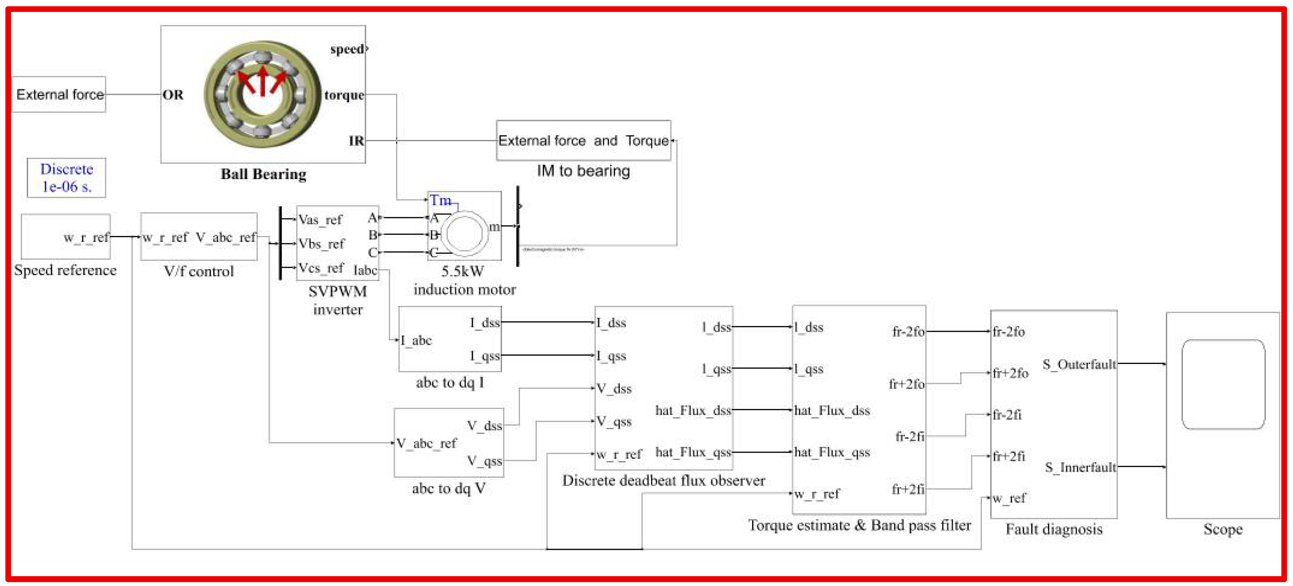
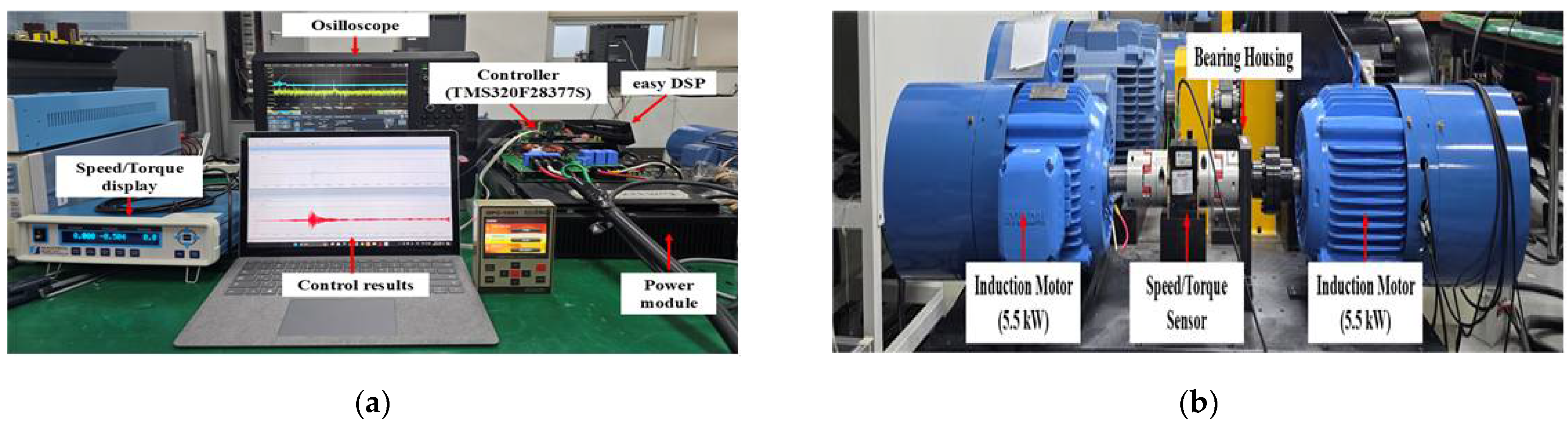
In contrast to conventional methods that depend on sophisticated signal transformation techniques, external sensors, or large-scale data-driven models, the presented method is computationally efficient and particularly suitable for embedded system deployment. The effectiveness of the approach was validated through MATLAB/Simulink (version 2024a) simulations as well as experimental investigations on a 5.5 kW motor-generator (M-G) setup.

2. Structure and Mathematical Modeling of the Induction Motor

2.1. Structure and Characteristics of the Induction Motor

An induction motor mainly comprises two principal elements: the stator and the rotor. The stator consists of laminated iron cores and distributed windings, which are supplied with an external AC voltage to produce a rotating magnetic field. This rotating field induces currents in the rotor by electromagnetic induction, thereby producing mechanical torque. Rotors are mainly divided into two categories: wound rotors and squirrel-cage rotors. Wound rotors are equipped with windings linked via slip rings and brushes, permitting external resistances to be inserted into the rotor circuit for torque adjustment and speed control. However, this design results in increased structural complexity and greater maintenance needs. By contrast, squirrel-cage rotors are formed from conductive bars that are short-circuited by end rings and embedded in the rotor core, removing the need for slip rings and brushes. This construction provides improved mechanical durability and decreased maintenance. As a result of these benefits, squirrel-cage induction motors are widely used in industrial environments. When compared to synchronous motors employing vector control, induction motors display more intricate dynamic characteristics owing to their nonlinear behavior dependent on slip. This increased complexity is particularly significant for torque estimation and observer-based control methodologies, where an accurate representation of rotor dynamics plays a critical role.

2.2. Mathematical Modeling of the Induction Motor

Equations (1) and (2) describe the voltage equations for both the stator and rotor components of induction motors:

$$V_s=R_s{I}_s+{\displaystyle \frac{d{\psi }_s}{dt}}$$

(1)

$$V_r=R_r{I}_r+{\displaystyle \frac{d{\psi }_r}{dt}}$$

(2)

where $V_s$ and $V_r$ represent the stator and rotor voltages, $R_s$ and $R_r$ denote the stator and rotor resistances, $I_s$ and $I_r$ indicate the stator and rotor currents, and ${\psi }_s$ and ${\psi }_r$ correspond to the stator and rotor flux linkages, respectively.

Equations (3) and (4) specify the stator-referenced d-axis and q-axis fluxes, respectively:

$${\psi }_{sd}=\int \left(v_{sd}-R_s{i}_{sd}\right)dt$$

(3)

$${\psi }_{sq}=\int \left(v_{sq}-R_s{i}_{sq}\right)dt$$

(4)

where ${\psi }_{sd}$ and ${\psi }_{sq}$ represent the stator-referenced d-axis and q-axis fluxes, $v_{sd}$ and $v_{sq}$ are the stator-referenced d-axis and q-axis voltages, and $i_{sd}$ and $i_{sq}$ represent the stator-referenced d-axis and q-axis currents, respectively.

Equation (5) presents the mechanical torque in terms of the stator d-axis and q-axis currents and fluxes, where $T_e$ denotes the mechanical torque, and $P$ indicates the number of poles:

$$T_e={\displaystyle \frac{3}{2}}{\displaystyle \frac{P}{2}}({\psi }_{sd}{i}_{sq}-{\psi }_{sq}{i}_{sd})$$

(5)

3. Bearing Fault Diagnosis

3.1. Ball Bearing

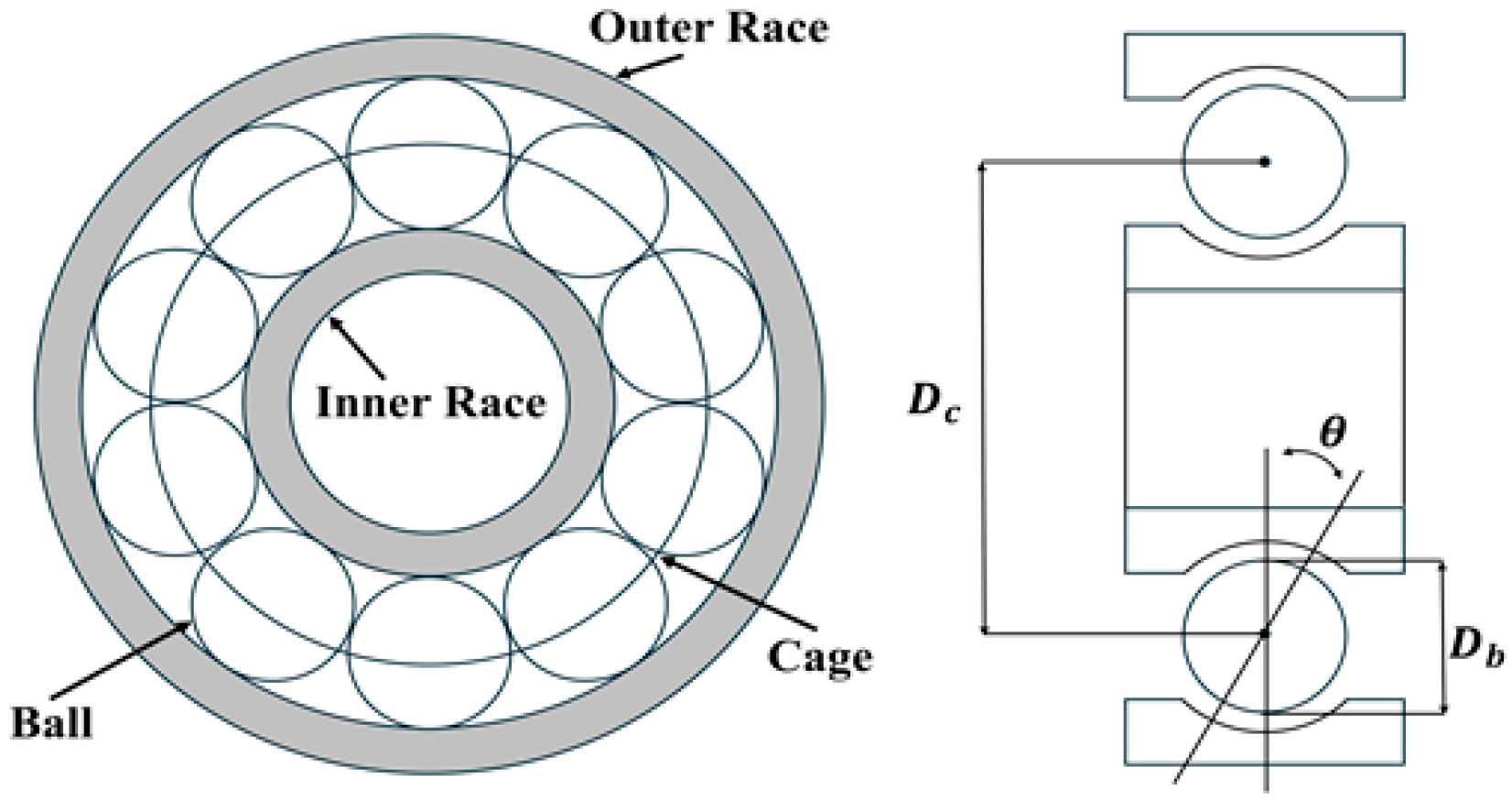
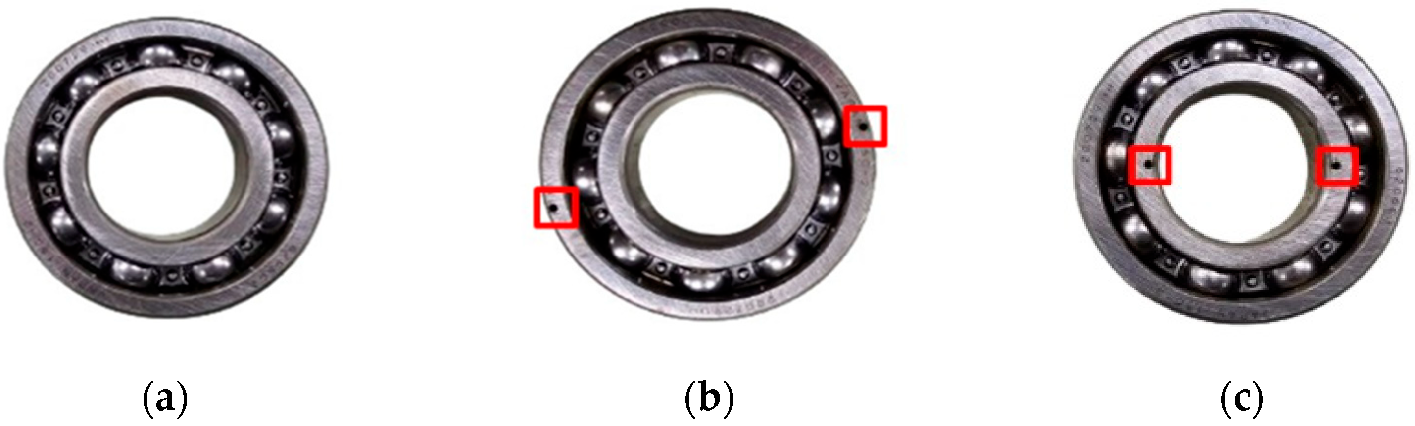
Bearings are mechanical elements that provide support for rotational or linear motion, minimizing friction and sustaining applied loads. Among the various types, ball bearings and roller bearings are the most prevalent. Specifically, radial ball bearings, also referred to as deep groove bearings, are extensively used for their capacity to operate at high rotational speeds while supporting radial and axial loads from different directions. A standard radial ball bearing comprises an outer race, inner race, balls, and a cage. The balls are positioned within deep grooves machined into the inner and outer races, ensuring stable operation during high-speed motion. Figure 1 shows the construction of the radial ball bearing considered in this work. The main geometric characteristics, including the ball diameter $D_b$, the pitch diameter $D_c$, and the contact angle $\theta$, significantly affect the vibration response and calculation of fault frequencies.

Table 1. Bearing 6206C3 Parameters.

Parameter	Value	Unit
Ball Diameter	8.1	mm
Pitch Diameter	46	mm
Width	16	mm
Number of Ball	9	-

summarizes the parameters of the NTN 6206C3 radial ball bearing used in this study.

3.2. Fault Frequencies in Ball Bearings

During rotation, defects such as cracks or wear on the outer race, inner race, balls, or cage can generate periodic contact between the rolling elements and the defect location. Such defects induce vibrations at characteristic frequency ranges, known as fault frequencies. The fault frequencies observed in vibration analysis are determined by parameters including bearing geometry, defect location, and rotational speed, as described by Equations (6)–(9) [4].

$$F_o={\displaystyle \frac{N_b}{2}}{F}_r(1-{\displaystyle \frac{D_{b}cos\theta }{D_c}})$$

(6)

$$F_i={\displaystyle \frac{N_b}{2}}{F}_r(1+{\displaystyle \frac{D_{b}cos\theta }{D_c}})$$

(7)

$$F_b={\displaystyle \frac{D_c}{D_b}}{F}_r[1-{\left({\displaystyle \frac{D_{b}cos\theta }{D_c}}\right)}^2]$$

(8)

$$F_c=F_r(1-{\displaystyle \frac{D_{b}cos\theta }{D_c}})$$

(9)

where $F_o$, $F_i$, $F_b$, and $F_c$ represent the fault frequencies associated with the outer race, inner race, balls, and cage, respectively; $F_r$ denotes the rotational frequency, and $N_b$ is the number of balls. These fault frequencies in the vibration domain also influence the stator current, with the corresponding fault frequencies in the current domain described by Equation (10):

$$F_{cur}=\left|F_r\pm k{F}_{vir}\right|$$

(10)

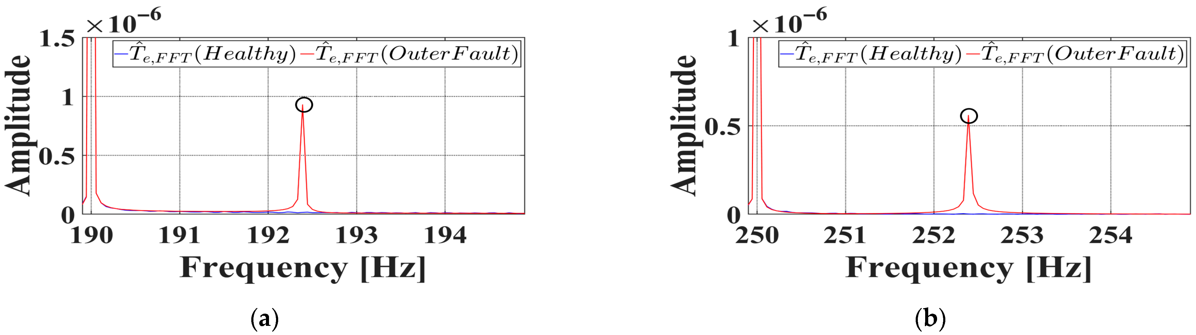
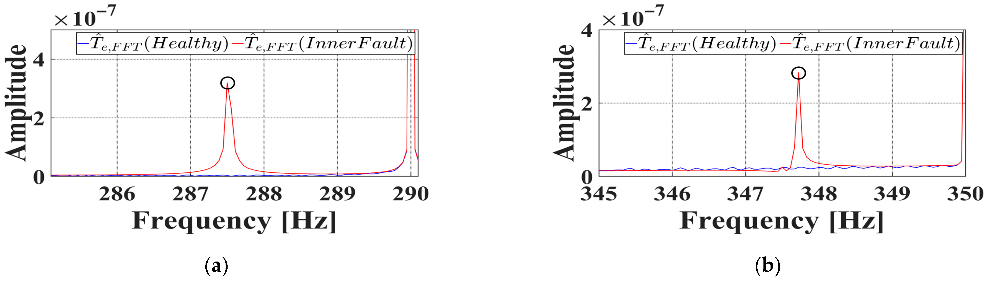
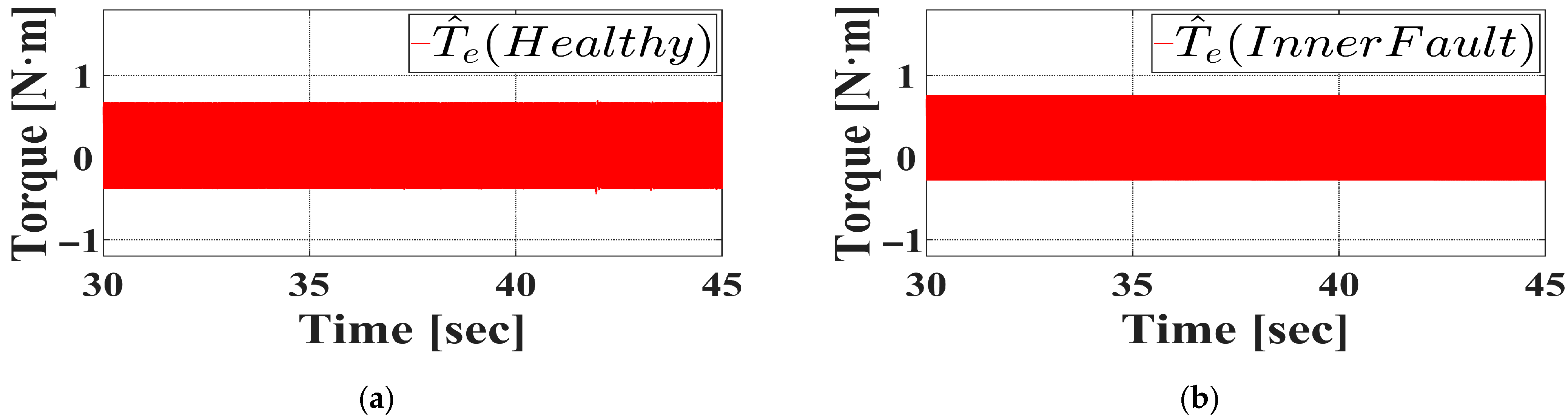
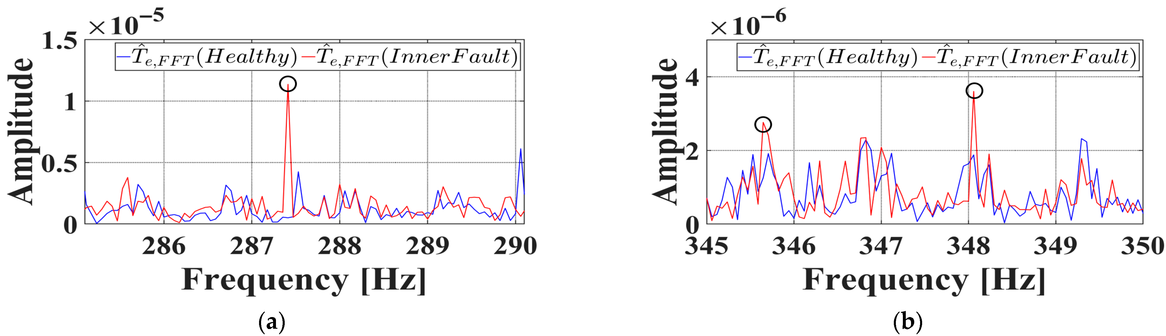
where $F_{cur}$ indicates the fault frequency in the current domain, $F_{vir}$ represents the vibration frequency as determined from Equations (6)–(9), and k is a constant parameter. The value of k may be chosen arbitrarily (e.g., k = 0, 1, 2, …). In this investigation, k was determined through experimental comparison of the FFT results calculated offline for healthy and faulty bearing torque. The selected k corresponds to a frequency component that reliably demonstrates a notably greater amplitude in faulty bearings relative to healthy units.

Table 2. Fault Frequency for 6260C3 Bearing.

${\mathit{F}}_{\mathit{r}}$	30 [Hz]	40 [Hz]
$\left|F_r-2F_o\right|$	192.4	256.5
$\left|F_r+2F_o\right|$	252.4	336.5
$\left|F_r-2F_i\right|$	287.6	383.5
$\left|F_r+2F_i\right|$	347.6	463.5

lists the calculated fault frequencies for the 6206C3 bearing model at different rotational frequencies.

3.3. Torque Observer

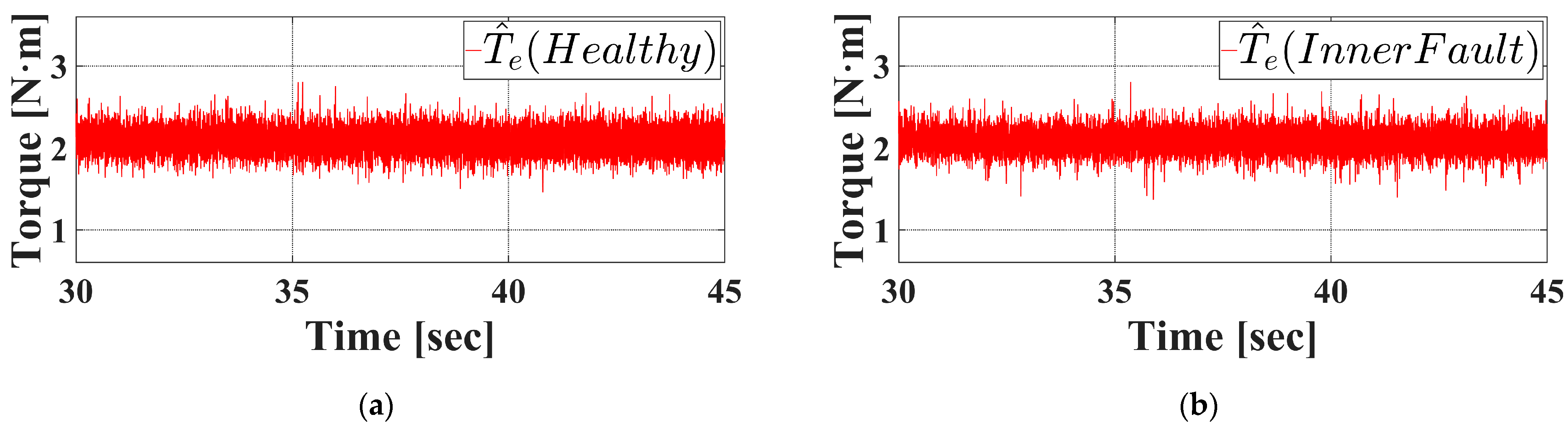
Previous research has generally relied on supplementary hardware, such as vibration sensors or accelerometers, to analyze vibration signals, thereby increasing the complexity and cost of maintenance. The analysis of current signals requires the application of online FFT, which is computationally intensive and demands extensive programming efforts. In contrast, this paper presents a streamlined fault diagnosis algorithm that utilizes the observed torque, relying only on offline FFT results obtained from a single calculation. The torque observer is derived from the full-order flux observer model associated with the induction motor [23]. Equation (11) defines the stator-referenced model of the induction motor:

$${\displaystyle \frac{d}{dt}}\left[\begin{array}{c}{\overrightarrow{i}}_s\\ \overrightarrow{{\psi }_s}\end{array}\right]=\left[\begin{array}{c}\begin{array}{cc}{A}_{11}& A_{12}\end{array}\\ \begin{array}{cc}{A}_{21}& A_{22}\end{array}\end{array}\right]\left[\begin{array}{c}{\overrightarrow{i}}_s\\ \overrightarrow{{\psi }_s}\end{array}\right]+\left[\begin{array}{c}{B}_1\\ B_2\end{array}\right]\overrightarrow{v_s}$$

(11)

Equation (12) provides the derivation for the full-order observer:

$${\displaystyle \frac{d}{dt}}\left[\begin{array}{c}\widehat{{\overrightarrow{i}}_s}\\ \widehat{\overrightarrow{{\psi }_s}}\end{array}\right]=\left[\begin{array}{c}\begin{array}{cc}{A}_{11}& A_{12}\end{array}\\ \begin{array}{cc}{A}_{21}& A_{22}\end{array}\end{array}\right]\left[\begin{array}{c}\widehat{{\overrightarrow{i}}_s}\\ \widehat{\overrightarrow{{\psi }_s}}\end{array}\right]+\left[\begin{array}{c}{B}_1\\ B_2\end{array}\right]\overrightarrow{v_s}\left[\begin{array}{c}{G}_1\\ G_2\end{array}\right](\widehat{{\overrightarrow{i}}_s}-{\overrightarrow{i}}_s)$$

(12)

where $A_{11}=-\left({\displaystyle \frac{R_s^{*}}{\sigma L_s}}\right)I+\omega J$, $A_{12}=\left({\displaystyle \frac{R_r}{\sigma L_s{L}_r}}\right)I-\left({\displaystyle \frac{\omega }{\sigma L_s}}\right)J$, $A_{21}=-R_{s}I$, $A_{22}=\overrightarrow{0}$, $B_1=\left({\displaystyle \frac{1}{\sigma L_s}}\right)I$, $B_2=I$, $G_1=A_{11}+A_{12}-K{A}_{21}$, $G_2=\left(1-K\right)A_{21}$, $K=5\left({\displaystyle \frac{R_r}{\sigma L_s{L}_r{R}_s}}\right)$, $R_s^{*}=R_s+{\displaystyle \frac{L_s{R}_r}{L_r}}$, $\sigma =1-{\displaystyle \frac{M^2}{L_s{L}_r}}$, $I=\left[\begin{array}{c}\begin{array}{cc}1& 0\end{array}\\ \begin{array}{cc}0& 1\end{array}\end{array}\right]$, $J=\left[\begin{array}{c}\begin{array}{cc}0& -1\end{array}\\ \begin{array}{cc}1& 0\end{array}\end{array}\right]$, and $\overrightarrow{0}=\left[\begin{array}{c}\begin{array}{cc}0& 0\end{array}\\ \begin{array}{cc}0& 0\end{array}\end{array}\right]$.

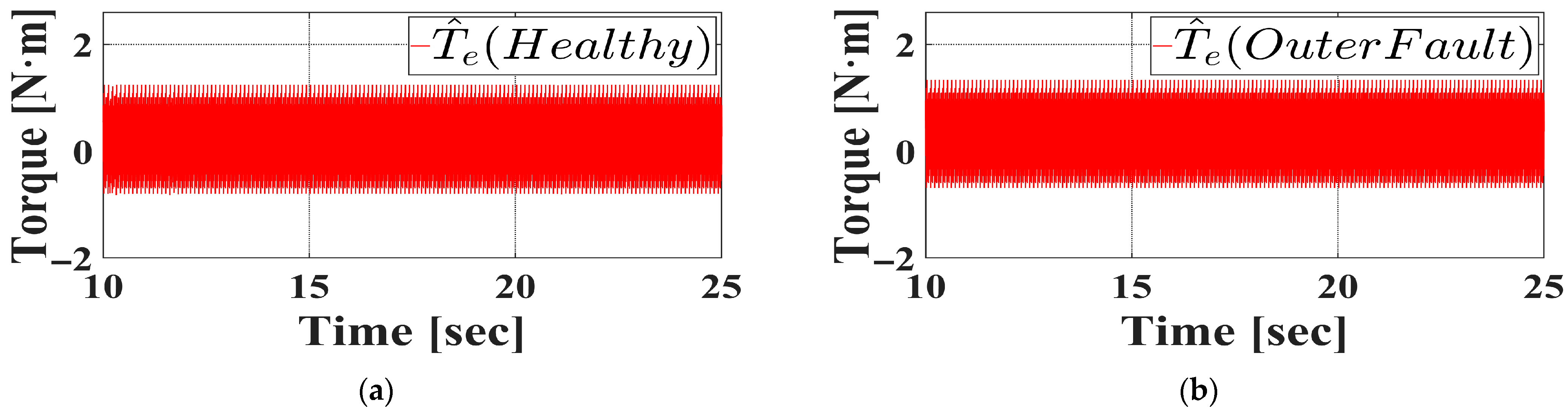
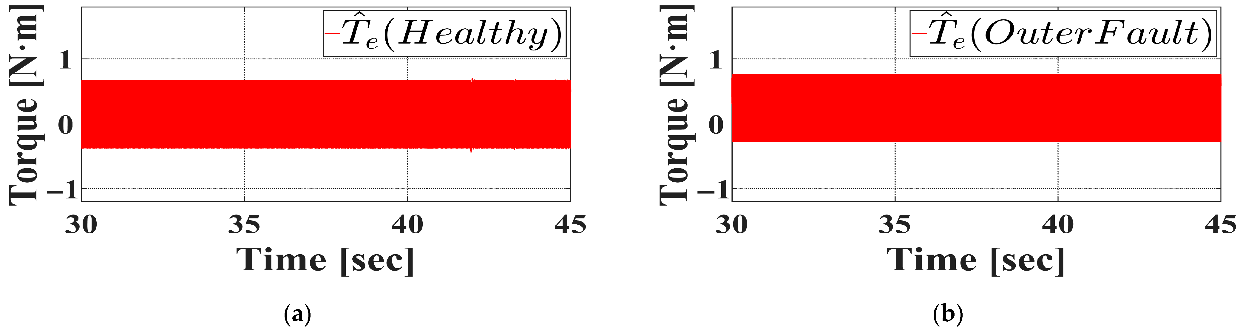
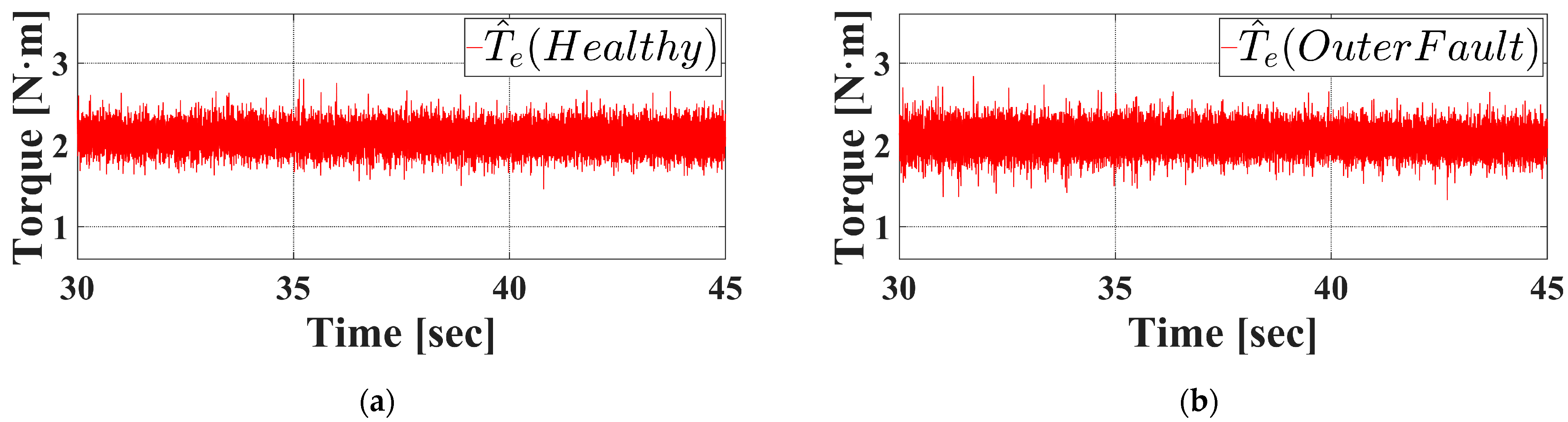
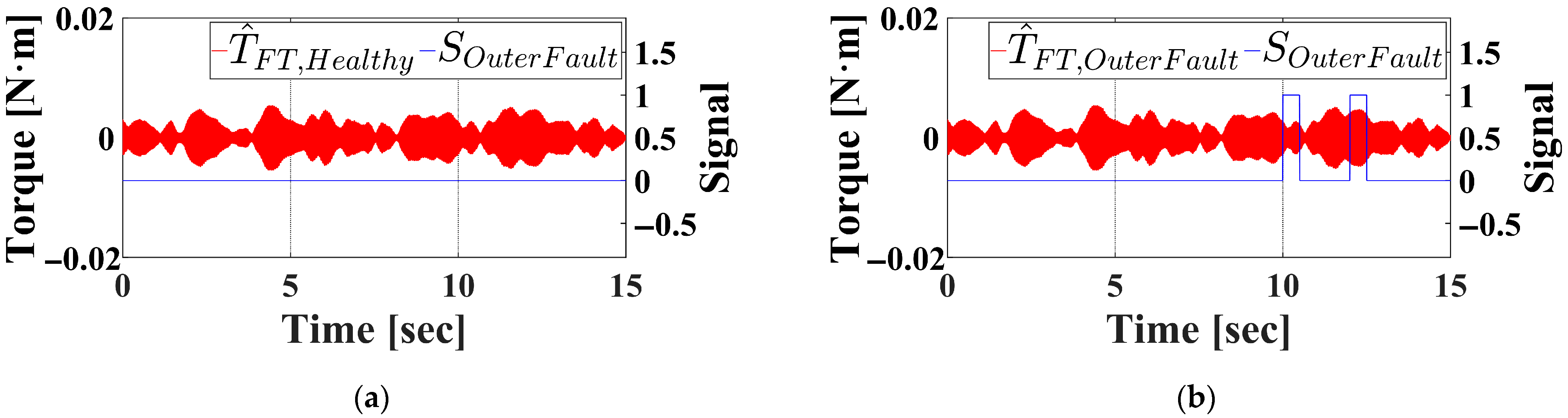
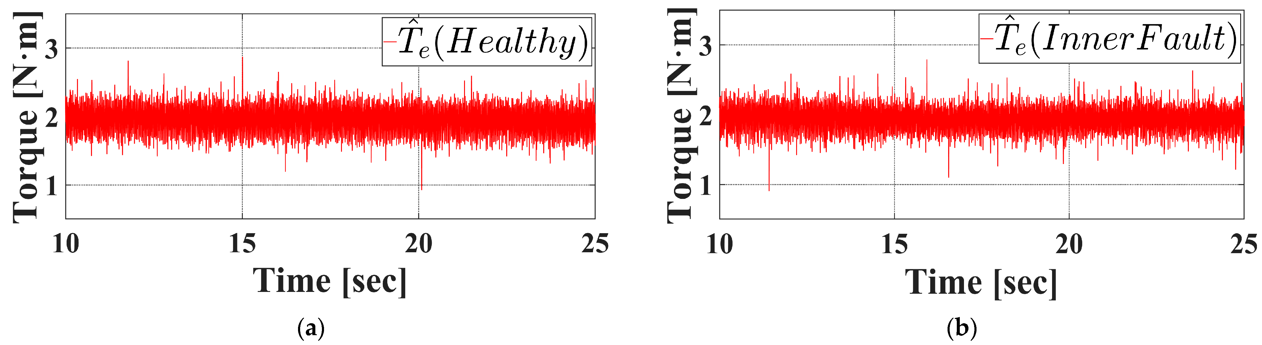
With the observed currents and flux from Equation (12), torque ${\widehat{T}}_e$ is determined using Equations (5) and (12). The computed torque signal is subsequently processed with a band-pass filter, and variations caused by bearing faults are assessed for diagnostic purposes.

3.4. Band-Pass Filter Design

Traditional fault diagnosis approaches frequently utilize FFT analysis for vibration or current signals. In this work, a band-pass filter is constructed based on the theoretical fault frequencies established in Equations (6)–(9) to facilitate real-time fault identification. Filters may be categorized as low-pass, high-pass, band-pass, or band-stop. Of these, a band-pass filter is employed in this study to selectively extract signal components within designated frequency intervals corresponding to diagnostic fault frequencies.

Equation (13) defines the transfer function for a second-order series $RLC$ band-pass filter as follows:

$$H\left(s\right)={\displaystyle \frac{RCs}{LC{s}^2+RCs+1}}$$

(13)

Here, $R$, $L$, and $C$ denote the resistance, inductance, and capacitance parameters of the filter, respectively. The filter’s resonant angular frequency and bandwidth are described as follows:

$$\left\{\begin{array}{c}{\omega }_0={\displaystyle \frac{1}{\sqrt{LC}}}\\ bandwidth={\displaystyle \frac{R}{L}}\end{array}\right.$$

(14)

To facilitate calculations, the resistance $R$ was assigned a value of 1 kΩ, and the bandwidth was specified as 5 Hz, yielding an inductance $L$ of 200 H. The value of capacitance $C$ was determined so that the filter’s resonant frequency could adapt to bearing fault frequencies, which vary with the motor speed from 1 Hz up to 60 Hz. Each corresponding value of $C$ for a given fault frequency was precomputed and stored in a look-up table. This configuration allows the filter to extract fault-specific components from the torque signal in real time as the fault frequency band shifts according to the changing motor rotational speed.

Before the designed filter can be operated online within a computer, the continuous-time system must be converted into a discrete-time system. This process can utilize transformation approximation methods or numerical integration approaches. Among these, numerical integration maintains the frequency response characteristics of the original continuous-time transfer function and is therefore widely adopted for discrete-time filter implementation. In this study, the Tustin numerical integration technique was chosen. Tustin’s Method involves replacing $s$ in the Laplace transform transfer function $H\left(s\right)$ with the corresponding expression from Equation (15), which is then rearranged to derive the discrete-time transfer function $H(z$) [24]:

$$s={\displaystyle \frac{2}{h}}{\displaystyle \frac{z-1}{z+1}}$$

(15)

In this context, $h$ refers to the sampling period, which is set to 0.1 ms for this investigation. Incorporating the expression from Equation (15) into Equation (14) produces Equation (16), which, upon further simplification, yields Equation (17):

$$H\left(z\right)={\displaystyle \frac{RC\left(\frac{2}{h}\frac{z-1}{z+1}\right)}{LC{\left(\frac{2}{h}\frac{z-1}{z+1}\right)}^2+RC\left(\frac{2}{h}\frac{z-1}{z+1}\right)+1}}$$

(16)

$$H\left(z\right)={\displaystyle \frac{G_3{z}^2-G_3}{z^2+G_{1}z+G_2}}$$

(17)

In these equations, $G_1={\displaystyle \frac{2-\frac{8LC}{h^2}}{\frac{4LC}{h^2}+\frac{2RC}{h}+1}}$, $G_2={\displaystyle \frac{\frac{4LC}{h^2}-\frac{2RC}{h}+1}{\frac{4LC}{h^2}+\frac{2RC}{h}+1}}$, and $G_3={\displaystyle \frac{\frac{2RC}{h}}{\frac{4LC}{h^2}+\frac{2RC}{h}+1}}$ have the indicated definitions.

The relationship between input and output described by $H\left(z\right)$ is divided by its denominator to express the output $y\left[n\right]$ in terms of previous samples. The discrete-time difference equation suitable for digital processing is presented in Equation (18):

$$y\left[n\right]=-G_{1}y\left[n-1\right]-G_{2}y\left[n-2\right]+G_{3}x\left[n\right]-G_{3}x[-2]$$

(18)

Here, $n$ indicates the discrete-time index. By feeding the observed torque signal from Equation (5) as the input $x\left[n\right]$ in Equation (18), the torque signal components within the fault frequency band can be efficiently extracted and used for diagnostic purposes.

3.5. Fault Diagnosis Algorithm

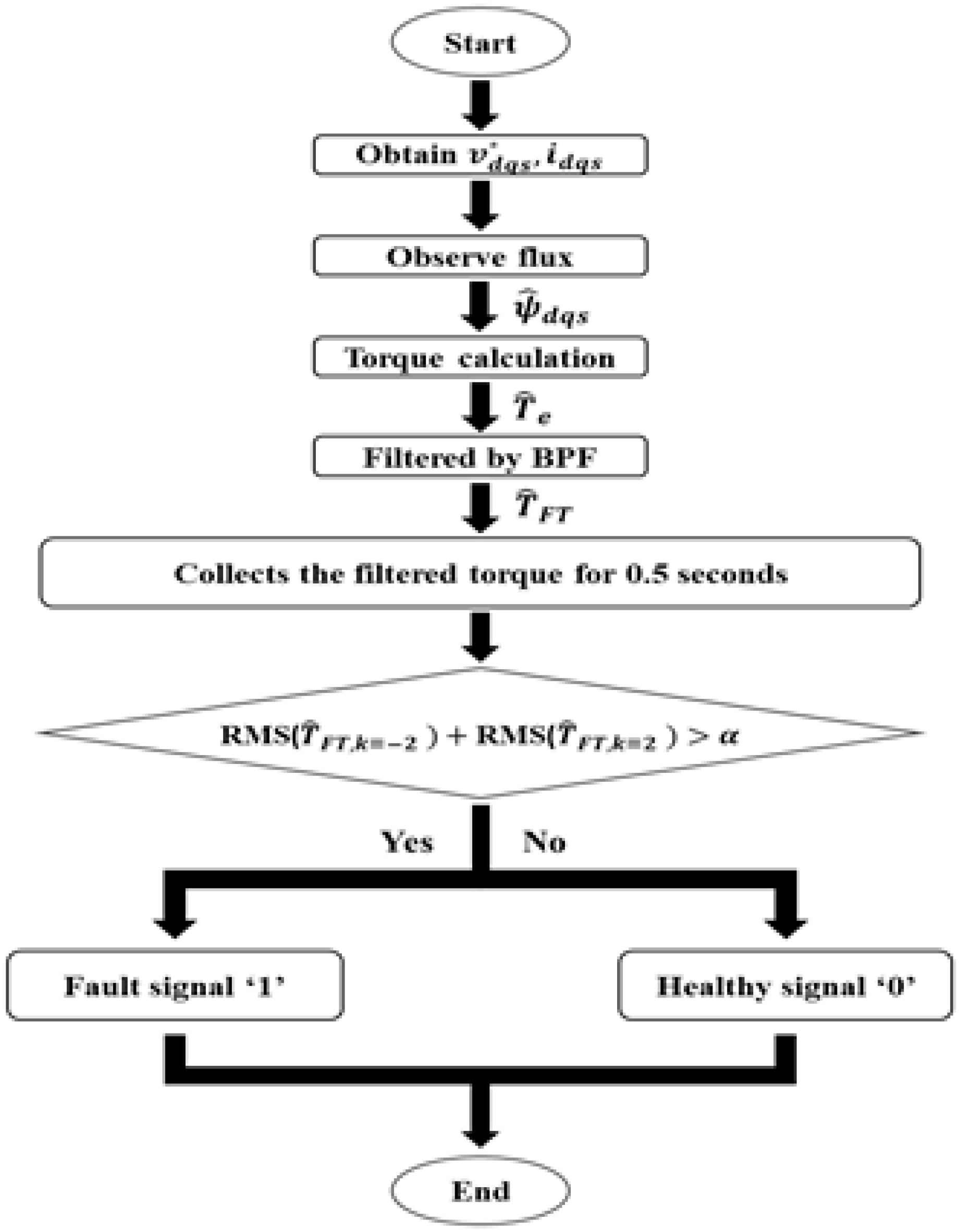
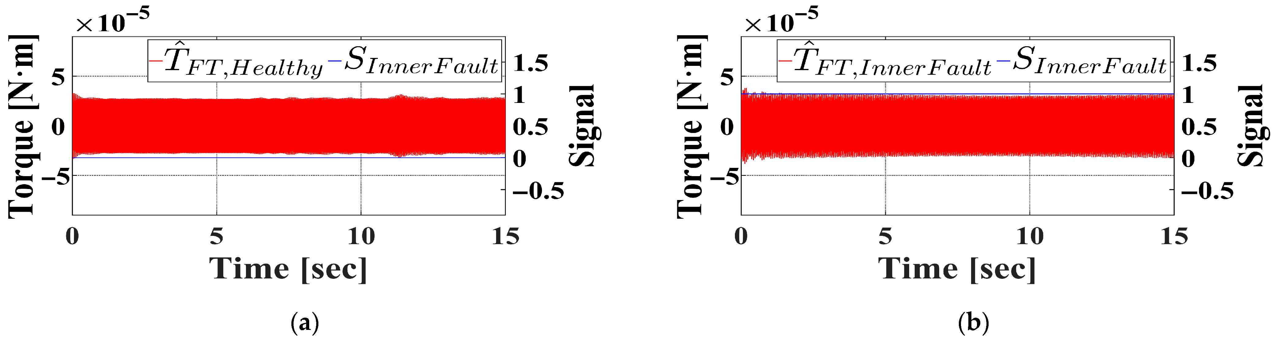
Figure 2 presents a flowchart of the fault diagnosis algorithm. In this flowchart, ${\widehat{\psi }}_{dqs}$ indicates the observed d-q axis stator flux, and ${\widehat{T}}_e$ represents the observed torque. ${\widehat{T}}_{FT}$ is the band-pass filtered torque utilized for fault detection, while $\alpha$ serves as the threshold value for diagnosing bearing faults. Specifically, ${\widehat{T}}_{FT, k=-2}$ and ${\widehat{T}}_{FT, k=2}$ indicate the filtered torque components related to the fault frequency bands at $k=-2$ and $k=2$ in Equation (10), respectively. The threshold $\alpha$ is determined from the maximum value of the filtered torque within the relevant fault frequency bands under healthy bearing conditions, as identified through experimental studies.

As discussed in Section 3.2, the bearing fault frequencies vary depending on the bearing geometry, defect location, and rotational speed. This implies that even under identical control conditions, the fault-related frequency components differ from one system to another. Consequently, the amplitude of the band-pass-filtered torque at the corresponding fault frequencies also varies, making statistical optimization of the threshold α impractical.

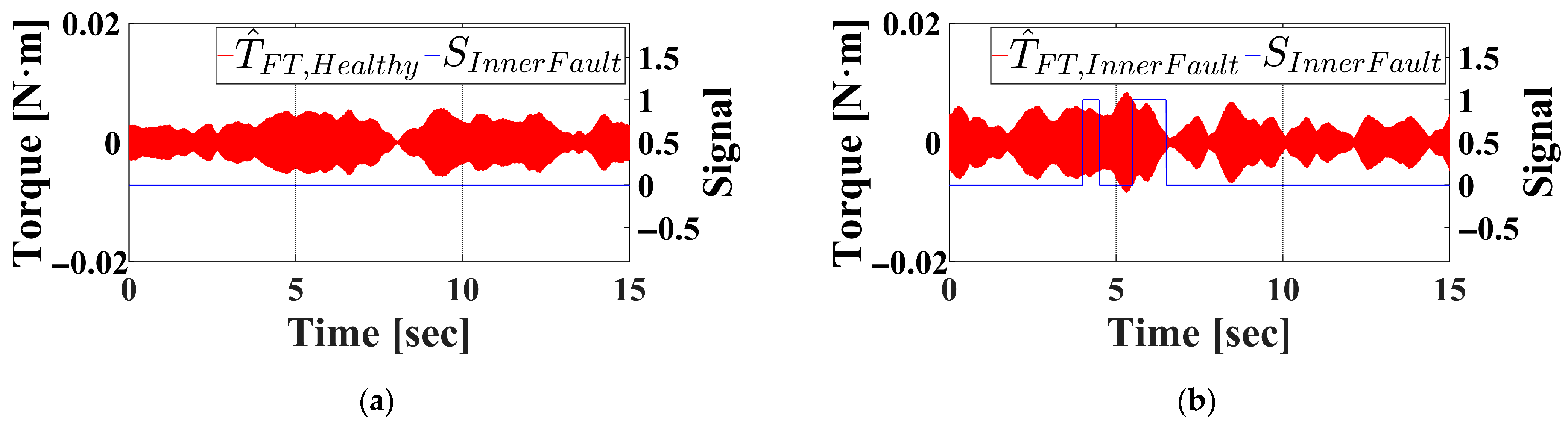
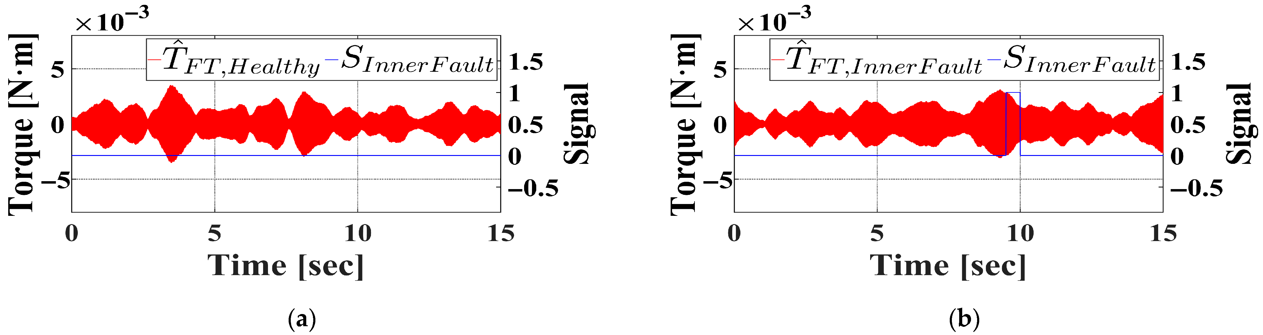
Prior to fault diagnosis, a preliminary procedure is performed to determine the threshold under healthy operating conditions. This procedure follows the same signal-processing sequence as the fault-diagnosis algorithm up to the computation of the two RMS values corresponding to $k=\pm 2$. During a 20 s healthy-state measurement, the maximum value of the summed RMS signal is identified, and the threshold $\alpha$ is empirically set to 1.1 times this maximum, as defined in Equation (19).

$$\alpha =1.1\times \mathrm{m}\mathrm{a}\mathrm{x}\{\mathrm{R}\mathrm{M}\mathrm{S}\left({\widehat{T}}_{FT, k=-2}\right)+RMS\left({\widehat{T}}_{FT, k=2}\right)\}$$

(19)

Similar to recent adaptive condition monitoring research, where non-static or system-specific thresholds are applied to improve robustness against variations in operating conditions [25], the empirically defined threshold in this study provides a safety margin that ensures reliable fault detection without false alarms during normal operation.

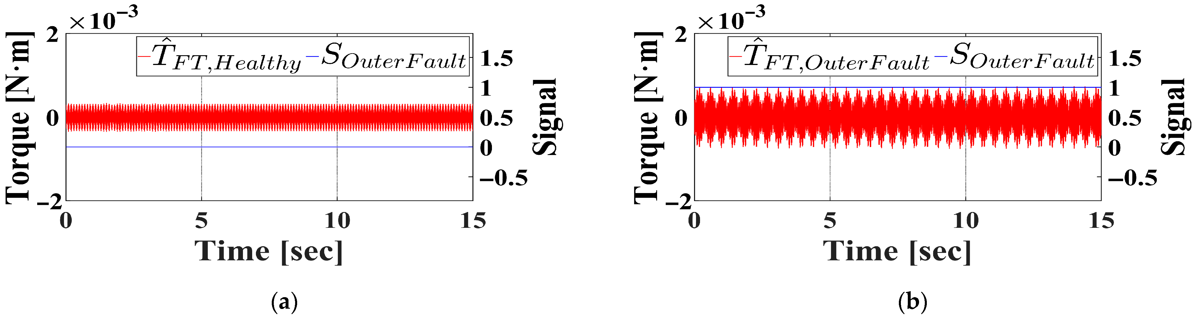
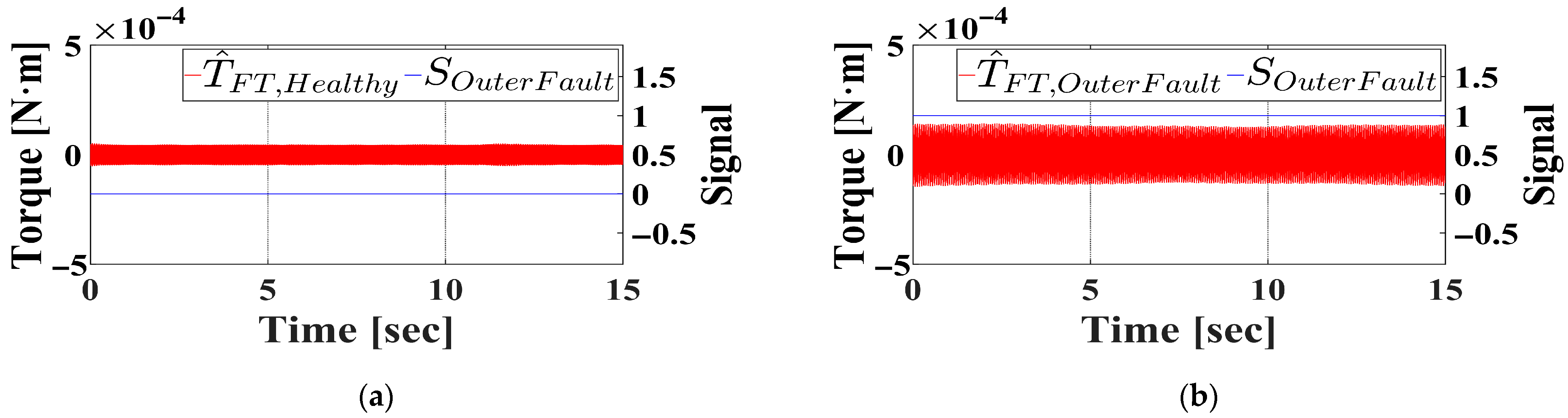
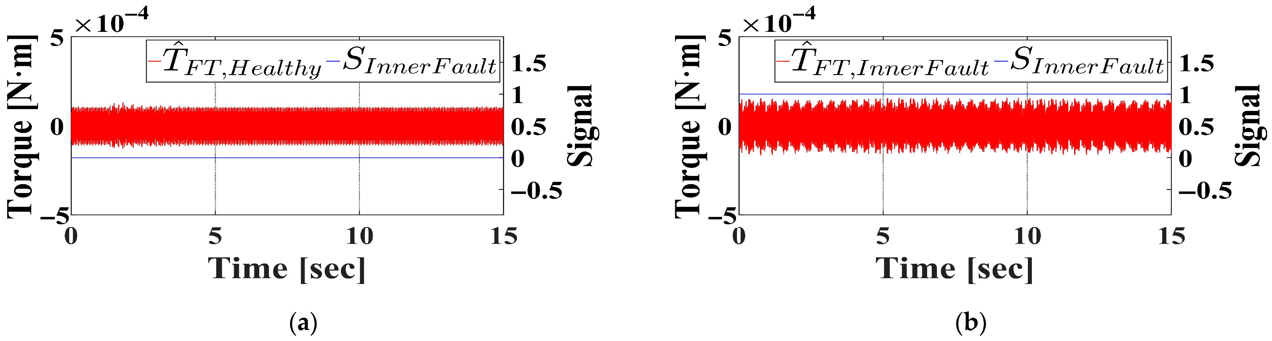
The fault diagnosis algorithm utilizes the commanded voltage and output current from the V/f controller and inverter to observe the d–q axis stator flux. Using this observed flux, the algorithm calculates the observed torque, which is then filtered through two BPFs with center frequencies corresponding to the fault frequency bands defined in Equation (10). In the current study, the frequency bands at $k=-2$ and $k=2$ are specifically analyzed. For each filtered torque signal, ${RMS}_{digital}$ value is defined as computed over a 0.5 s window (sampling period = 0.1 ms) as described in Equation (20), and the two RMS values for $k=-2$ and $k=2$ are summed. This total is subsequently compared to the fault detection threshold α. If the total exceeds α, the algorithm outputs a fault signal ‘1’, otherwise, it outputs a healthy signal ‘0’.

In practical industrial applications, the threshold α is predefined according to the healthy operating characteristics of each drive system. Since small variations inevitably exist among motors and bearings due to manufacturing tolerances or installation conditions, a minor preset adjustment of the threshold enables stable and consistent fault detection across systems. This approach reflects a realistic implementation strategy commonly adopted in industrial control, offering robustness and simplicity without the need for adaptive or AI-based tuning. The proposed method is intended to complement existing industrial monitoring systems rather than replace them. It provides an additional diagnostic layer that enhances fault detectability without requiring any major modification to current control architectures.

$${RMS}_{digital}=\sqrt{{\displaystyle \frac{1}{5000}}\sum _{n=1}^{5000}{y\left[n\right]}^2}$$

(20)

4. Simulation Configuration and Result

4.1. Simulation Configuration

Figure 3 shows the comprehensive simulation system implemented in MATLAB/Simulink. The system includes modules for induction motor control, a bearing model, a torque observer used in fault detection, a band-pass filter, and a fault diagnosis unit. The simulation utilizes a 5.5 kW induction motor model along with an NTN 6206C3 radial ball bearing model. The bearing model, sourced from the Simulink library, offers a standardized representation of radial ball bearings. This study investigates bearing faults, including cracks and pits on the outer and inner races. However, such physical damages cannot be directly modeled in the Simulink library. To address this, damaged bearings were used in initial physical experiments, and the simulation replicated these fault effects by adjusting parameters such as friction and damping within the bearing model. This approach, based on parameter adjustments, allowed the simulation results to closely match those from physical experiments, affirming the validity of the simulation technique for bearing fault diagnosis.

Figure 4 illustrates the motor speed profile implemented in the simulation, where the speed command was incremented in discrete steps to evaluate fault diagnosis capabilities under varying operational states. The motor accelerates to 1800 rpm within the initial 5 s, holding at this speed for 20 s; it then ramps up to 2400 rpm, maintaining this speed for an additional 20 s. As fault frequencies are influenced by motor speed, only two characteristic speeds (1800 rpm and 2400 rpm) were chosen for in-depth investigation.

4.2. Outer Race Fault Simulation Result

Due to the speed dependence of fault frequency components, fault diagnosis utilizes the steady-state segments of the observed torque signal. Figure 5a displays the steady-state observed torque (from 10 to 25 s) at 1800 rpm for a healthy bearing, and Figure 5b presents the corresponding signal for an outer-race faulty bearing. It is evident that clear differentiation between healthy and faulty cases, even under steady-state conditions, remains difficult when relying solely on time-domain waveforms. Because the signal formats are very similar, even magnified time-domain waveforms cannot provide reliable distinction between healthy and faulty conditions. Therefore, we filter out frequency components that do not contain fault-related information.

To distinguish between healthy and faulty bearings, frequency-domain analysis was performed on the observed torque signals during steady-state operation at 1800 rpm. As bearing defects induce modulation of the torque signal at specific frequencies, FFT was applied to extract spectral features using a single offline calculation. Figure 6 presents a comparative analysis of FFT results for both conditions. The blue curve corresponds to the FFT of the observed torque for a healthy bearing, while the red curve represents that of a bearing with an outer-race fault. Pronounced amplitude differences are observed at 192.4 Hz and 252.4 Hz, which correspond to fault characteristic frequencies at k = ±2.

Drawing from these findings, two band-pass filters (BPFs) centered at the critical frequencies (k = ±2) were designed and applied to the observed torque. Without performing real-time FFT, the filter outputs were summed and analyzed in comparison. As a result, the filtered torque signal of the faulty bearing exhibited larger magnitudes and more prominent periodic spikes than that of the healthy bearing, providing a clear basis for fault detection.

When the proposed fault diagnosis algorithm is applied to the filtered signals, Figure 7a,b present the filtered torque signals together with the corresponding binary fault diagnosis outputs for the healthy and outer-race faulty bearings. The healthy bearing yields a fault signal of 0, whereas the faulty bearing yields a fault signal of 1, thereby verifying the effectiveness of the proposed detection method.

The procedure was repeated at a motor speed of 2400 rpm. In Figure 8a, the observed torque signal for the healthy bearing is shown, while Figure 8b depicts the corresponding signal for the outer race faulty bearing. Similar to the results at 1800 rpm, it remains difficult to reliably distinguish bearing faults using only the time-domain waveforms at this higher speed.

At the increased rotational speed, the characteristic fault frequencies shifted to 256.5 Hz and 336.5 Hz. The observed torque signal was processed using two band-pass filters centered at these frequencies, and the filter outputs were summed. After applying the proposed fault diagnosis algorithm to this summed signal, the outcomes for the healthy and outer race faulty bearings are provided in Figure 9a and Figure 9b, respectively. Here, the faulty bearing shows higher amplitude variations, and the algorithm successfully detects an outer race fault signal of ‘1’, thus confirming detection performance at elevated speeds.

4.3. Inner Race Fault Simulation Result

The fault diagnosis procedure was also applied for inner race fault detection. At a motor speed of 1800 rpm, observed torque signals were collected for both healthy and faulty bearings and are illustrated in Figure 10. The time-domain signals show that obvious distinctions between healthy and faulty cases are not visually evident, even under steady-state conditions.

Figure 11 displays the FFT analysis used to identify the modulated frequency components related to inner race faults. With a fault present, prominent amplitude modulations appear at 287.6 Hz and 347.6 Hz, which correspond to the fault frequencies at $k=\pm 2$. These frequencies provided the reference for designing the band-pass filters utilized in the subsequent fault diagnosis process.

The observed torque signal was processed using two band-pass filters centered at 287.6 Hz and 347.6 Hz, after which the outputs were summed. The processed signal was then evaluated by the proposed fault diagnosis algorithm. Figure 12a and Figure 12b present the results corresponding to the healthy and inner race faulty bearings, respectively. As illustrated, the faulty bearing demonstrates greater amplitude with distinct periodic spikes, allowing the algorithm to accurately produce a fault signal of ‘1’, thereby verifying the existence of an inner race fault.

At a motor speed of 2400 rpm, Figure 13a and Figure 13b display the observed torque signals for the healthy and the inner race faulty bearings, respectively. Similar to the observations at 1800 rpm, accurate diagnosis remains challenging under these conditions.

The observed torque signal underwent filtering through two band-pass filters centered at 383.5 Hz and 463.5 Hz, and the sum of the resulting outputs was computed. The fault diagnosis algorithm was subsequently implemented on this processed signal, with results shown in Figure 14a and Figure 14b for the healthy and inner race faulty bearings, respectively. The algorithm produces an inner race fault signal of ‘0’ for the healthy bearing and ‘1’ for the faulty one, thereby indicating successful detection of the fault at 2400 rpm.

5. Experimental Configuration and Result

5.1. Experimental Configuration

Figure 15a illustrates the experimental arrangement, highlighting the configuration of the control system. A PC, along with the easy DSP interface, was utilized to upload the motor control algorithm onto a TMS320F28377S digital signal processor (DSP). The motor operation was controlled manually using a keypad input. To ensure the reliability of the torque measurements, a torque sensor was connected to a Torque Display unit, which served as the reference standard for this experiment. The DSP’s analog output terminals were used for data acquisition, with signals captured and analyzed via an oscilloscope. Figure 15b depicts the M-G set deployed in the experiment. This arrangement includes two 5.5 kW induction motors: the right-side motor functions as the driving unit, while the left-side motor is typically assigned as the load. Even though the loading motor remained inactive during testing, it was kept mechanically engaged to enable torque sensor measurements. Additionally, the driving motor was equipped with a custom bearing housing to facilitate evaluation under both healthy and fault-induced bearing conditions.

Table 3. Induction Motor Parameters.

Parameter	Value	Unit
Rated Speed	3520	Rpm
Rated Power	5.5	kW
Rated Voltage	380	V
Rated Current	10.9	-A

summarizes the parameters of the induction motor utilized in the experimental study.

Figure 16 displays the bearings examined in this research. Figure 16a presents the healthy bearing, while Figure 16b and Figure 16c show bearings with an outer race fault and an inner race fault, respectively. The faulty bearings were prepared by drilling 2 mm holes at 180° intervals on both the outer and inner races to introduce faults. The red marks in the figures indicate the precise positions of these faults.

5.2. Outer Race Fault Experimental Result

Figure 17 illustrates the motor speed profile obtained from a speed sensor. The motor was subjected to the same stepwise speed sequence as used in the simulation, enabling performance comparison of the algorithm under realistic operational scenarios. The motor accelerates to 1800 rpm within the initial 5 s and sustains this speed for the subsequent 20 s. It then transitions to 2400 rpm and maintains this speed for another 20 s. Consistent with the simulation, only two key speeds (1800 rpm and 2400 rpm) were investigated experimentally as fault frequencies depend on the motor speed.

By examining the period from 10 to 25 s with the motor running at 1800 rpm, Figure 18a presents the observed torque for a healthy bearing, while Figure 18b shows the observed torque for a bearing with an outer-race fault. Despite closer inspection, the differences in the torque traces are not sufficiently evident to enable reliable bearing fault diagnosis from these signals alone. Because the signal formats are very similar, even magnified time-domain waveforms cannot distinguish between healthy and faulty conditions. Therefore, we filter out frequency components that do not contain fault-related information.

Figure 19 presents the FFT analyses used to identify the fault frequencies linked to bearing defects. Although FFT was performed for several $k$ values, the case with $k=\pm 2$ effectively differentiated healthy bearings from faulty ones. The blue curve indicates the FFT of the observed torque for the healthy bearing, and the red curve shows the result for the outer race faulty bearing. Clearly, the faulty bearing displays significantly greater peak magnitudes at the characteristic fault frequencies of 192.4 Hz and 252.4 Hz (i.e., $k=\pm 2$) relative to the healthy bearing.

Following FFT analysis, the torque signal was filtered using two band-pass filters, each centered at one of the identified frequencies, and the filter outputs were added. The amplitude variations in the resulting signal were more pronounced for the faulty bearing, signifying the emergence of fault-related modulations.

When the proposed diagnostic algorithm is applied to the filtered torque signals, the results are shown in Figure 20a and Figure 20b for the healthy and faulty bearings, respectively. In both plots, the filtered torque is plotted in red, while the binary fault indicator is given in blue. The algorithm produces an output of ‘0’ for a healthy bearing and ‘1’ for a faulty one, confirming its efficacy in clearly distinguishing between the two conditions.

The same procedure was applied to the interval from 30 to 45 s, during which the motor operated at 2400 rpm. Figure 21a and Figure 21b display the observed torque signals for both healthy and faulty bearings, respectively. As demonstrated, accurately diagnosing the bearing fault using only time-domain waveforms remains challenging, due to the minor differences observed between healthy and faulty signal characteristics.

Therefore, the observed torque signal is processed with two band-pass filters centered at 256.5 Hz and 336.5 Hz, then the filter outputs are summed. The proposed fault diagnosis algorithm is subsequently applied to this summed signal, and the results are illustrated in Figure 22a and Figure 22b for the healthy and faulty bearings, respectively. It is evident that the faulty bearing produces a noticeably higher amplitude compared to the healthy bearing. The diagnosis algorithm’s binary output verifies this finding by generating an outer race fault signal of ‘0’ for the healthy bearing and ‘1’ for the faulty bearing.

5.3. Inner Race Fault Experimental Result

Initially, during the interval from 10 to 25 s, when the motor ran at 1800 rpm, Figure 23a depicts the observed torque for the healthy bearing, while Figure 23b shows the corresponding signal for the bearing with an inner race fault. Despite examining magnified time-domain waveforms, distinguishing between healthy and faulty conditions based solely on observed torque remains unreliable due to insufficiently prominent distinguishing features.

Figure 24 illustrates the FFT results used to detect the characteristic fault frequencies. The blue trace shows the FFT of the observed torque for the healthy bearing, while the red trace depicts the result for the inner race faulty bearing. As depicted, at fault-related frequencies of 287.6 Hz and 347.5 Hz (i.e., $k=\pm 2$), the magnitude for the faulty bearing is substantially increased relative to the healthy bearing, confirming the appearance of fault-induced modulation components.

Accordingly, the measured torque signal is processed using two band-pass filters centered at 287.6 Hz and 347.5 Hz, and the resulting filtered signals are summed. Subsequently, the proposed fault diagnosis algorithm is implemented, with the corresponding results depicted in Figure 25a and Figure 25b for healthy and inner race faulty bearings, respectively. As illustrated, the faulty bearing demonstrates elevated amplitude levels with clearly periodic spikes, and the algorithm generates a fault signal of ‘1’, while the healthy bearing results in an output of ‘0’.

Figure 26a and Figure 26b display the observed torque signals corresponding to healthy and inner race faulty bearings, respectively, while the motor operates at 2400 rpm. While the faulty bearing reveals more pronounced abrupt changes in the torque waveform on closer examination, these variations by themselves are insufficient to allow a conclusive diagnosis in the time domain.

In this case, two band-pass filters centered at 383.5 Hz and 463.5 Hz are applied to the observed torque signal, with their corresponding filtered outputs subsequently summed and assessed. Figure 27a and Figure 27b show the outcomes obtained after implementing the proposed fault diagnosis algorithm for the healthy and inner race faulty bearings, respectively. The faulty bearing exhibits a clear increase in amplitude compared to the healthy scenario. Furthermore, the diagnosis algorithm outputs an inner race fault signal of ‘0’ for the healthy bearing, and ‘1’ for the faulty bearing, thereby verifying accurate fault detection.

6. Conclusions

This paper presents a sensorless fault diagnosis approach designed for reliable detection of bearing faults in induction motors. Initially, torque signals collected from both healthy and faulty bearings were examined in the frequency domain using FFT. The resulting analysis demonstrated that bearings with faults display substantially higher amplitudes in proximity to fault-specific frequency components relative to healthy bearings. Building on this finding, a BPF centered at the identified fault frequencies was implemented. The output from this filtering stage was subsequently analyzed by a lightweight, threshold-based algorithm for fault detection. The efficacy of the proposed technique was confirmed through MATLAB/Simulink simulations and experimental evaluations performed on a 5.5 kW M-G set. The algorithm effectively distinguished both inner and outer race faults at operational speeds of 1800 rpm and 2400 rpm. Major benefits of this approach include its sensorless configuration, minimal computational resource requirements, and exemption from the need for extensive training datasets or deep learning frameworks. In comparison with AI-based diagnostic models, the proposed method achieves practical and reliable bearing fault detection through simple signal observation and threshold evaluation, without relying on complex model training or parameter optimization. These attributes enhance its interpretability, reduce resource consumption, and make it particularly appropriate for practical, real-time embedded use cases. Consequently, this method provides a feasible and scalable strategy for bearing fault detection, especially in environments where employing numerous external sensors or high-end processors is financially impractical—such as sites deploying large fleets of induction motors. Future research will aim to broaden the applicability of the proposed algorithm through hybrid approaches that combine threshold-based diagnosis with trend analysis techniques. Collaborative industrial validation across diverse operating environments will also be pursued to further assess robustness and generalization. Additionally, future studies will explore the development of adaptive threshold algorithms, inspired by recent advances in dynamic condition monitoring methods.