Article

High-Performance Reservoir Simulation with Wafer-Scale Engine for Large-Scale Carbon Storage

1
National Energy Technology Laboratory, 626 Cochran Mill Road, Pittsburgh, PA 15236, USA
2
NETL Support Contractor, 626 Cochran Mill Road, Pittsburgh, PA 15236, USA
3
National Energy Technology Laboratory, 1450 SW Queen Ave, Albany, OR 97321, USA
4
NETL Support Contractor, 1450 SW Queen Ave, Albany, OR 97321, USA
5
National Energy Technology Laboratory, 3610 Collins Ferry Rd, Morgantown, WV 26505, USA
*
Authors to whom correspondence should be addressed.
Energies 2025, 18(22), 5874; https://doi.org/10.3390/en18225874
Submission received: 29 September 2025 / Revised: 30 October 2025 / Accepted: 5 November 2025 / Published: 7 November 2025
(This article belongs to the Special Issue Advances in Carbon Capture, Utilization & Storage (CCUS))

Abstract

Reservoir simulations are essential for subsurface energy applications, but remain constrained by the long runtimes of high-fidelity solvers and the limited generalizability of pretrained machine learning models. This study presents a multiphase reservoir simulator implemented on the Wafer Scale Engine (WSE), a new hardware architecture that delivers supercomputer performance on a single chip. Application development on the WSE is still at a nascent stage, and this study is, to our knowledge, the first to implement a full-physics, two-phase CO2-brine reservoir simulator on WSE, achieving runtimes on the order of seconds for reservoir-scale simulations while preserving full numerical accuracy. The developed simulator incorporates detailed physics for simulating CO2 transport in geological formations. As a case study, we considered CO2 injection into a field-scale reservoir model consisting of over 1.7 million cells. The WSE solver achieves more than two orders of magnitude speedup compared to a conventional CPU-based parallel simulator, completing a 5-year simulation in just 2.8 s. The WSE performance remained nearly unchanged to a four-fold increase in grid resolution, in contrast to the strong slowdown observed with the CPU-based solver. These findings provide the first proof-of-concept of wafer-scale computing for enabling high-resolution, large-scale full-physics simulations in near-real-time, overcoming the tradeoff between speed and accuracy and opening a new paradigm for carbon storage and broader subsurface energy applications.

1. Introduction

Reservoir simulation plays a pivotal role in subsurface energy applications such as carbon storage, enhanced oil recovery, and waterflooding. Accurate multiphase flow modeling provides critical insights into reservoir performance and supports-informed operational decisions. However, the scale and complexity of field systems impose heavy computational demands that make simulations challenging. Conventional full-physics simulators, despite their robustness and accuracy, often require prohibitively long runtimes, even when deployed on high-performance computing (HPC) clusters. The primary limitation arises from the communication and data transfer bottlenecks within these systems, which restrict the scalability and efficiency of large-scale simulations [1,2].
In recent years, reduced-order modeling (ROM) and machine learning (ML) have emerged as alternatives to accelerate reservoir simulations. Physics-informed, deep learning neural networks can approximate flow dynamics much faster than numerical solvers and have been successfully applied to tasks such as CO2 plume prediction and reservoir management [3,4]. However, these methods generally rely on large training datasets generated by high-fidelity simulators. In addition, generalizability to new reservoirs or new operating conditions remains a significant challenge and the underlying models often lack interpretability. Thus, while ML and ROM approaches offer speed, they cannot yet fully replace physics-based models for decision-critical applications.
This work seeks to bridge the long-standing tradeoff between accuracy and efficiency in reservoir simulation by leveraging the nascent wafer scale computing technology and the underlying wafer scale engine (WSE) hardware to build a highly scalable simulation framework. The resulting framework integrates the rigorous physics of conventional full-physics models with the computational speed typically offered by ML surrogates, creating a new paradigm for reservoir simulation in near-real time. In doing so, this framework lifts the speed limitation of traditional HPC solvers and the interpretability concern over data-driven ROM methods.
The developed simulator employs a finite-difference scheme to discretize the governing partial differential equations (PDEs) of CO2-brine flow and integrates advanced physical processes critical for storage applications. These include the Peng–Robinson EOS for pressure–volume–temperature (PVT) properties [5], Corey’s model for relative permeability [6], gravitational segregation from CO2-brine density differences, porosity–pressure coupling, and CO2 solubility in brine. All of these components were implemented from scratch for the WSE, using a special application programming interface (API). To demonstrate the potential of this framework, the simulator is applied to CO2 storage at the scale of the Illinois Basin Decatur Project (IBDP) site [7,8].
The remaining sections are organized as follows. Section 2 provides a review of full-physics simulators, reduced-order models, and machine learning approaches for subsurface flow modeling, as well as an introduction on wafer scaling computing. Section 3 introduces the two-phase flow problem formulation, the WSE technology, and the implementation of the WSE-based flow simulator. Section 4 and Section 5 show the three-dimensional benchmarking results and discussions, followed by the conclusions in Section 6.

2. Background

2.1. Speed Versus Accuracy in Reservoir Simulations

Numerical simulation of fluid flow in porous media has been extensively studied by researchers using models that are primarily centered around two approaches, full-physics simulators and reduced-order models. Full-physics simulators solve the governing partial differential equations (PDEs) of multiphase flow in porous media, incorporating representation of reservoir properties, fluid behaviors, and initial and boundary conditions. These simulators are built on well-established numerical methods, such as finite difference, finite volume, or finite element methods, and are widely considered robust because of their accuracy and broad energy applications [9,10,11]. At the reservoir-scale, running full-physics simulators on a single workstation can be computationally demanding due to significant processing time. High-performance computing (HPC) clusters, consisting of interconnected computing nodes, have been broadly employed to speed up the solution of large-scale reservoir models. As of November 2024, the fastest supercomputer (El Capitan located at the Lawrence Livermore National Laboratory) achieves 1.742 exaflops (1.742 × 10¹⁸ floating-point operations per second) [12]. Scaling efficiency of the HPC clusters, however, is limited by the data transfer speeds among its components, including storage (cache memory, random-access memory, and hard disk), network, and compute nodes.
To alleviate these challenges, various reduced-order modeling (ROM) methods, referring broadly to projection-based methods and surrogate modeling-based techniques, have been used to reduce the complexity of full-physics models through process simplification or alternative representation [13,14,15,16,17]. Machine learning (ML) has long been studied as a surrogate modeling technique [18,19]. In porous media modeling, the advent of deep learning in the recent decade has ignited strong interest in developing ML-based surrogate models as a fast alternative to fluid flow simulation prediction [16,20,21,22,23,24,25,26,27]. In general, various ML techniques seek to learn representations of domain input–output mappings or data patterns using artificial neural networks as computationally efficient approximators. For example, Zhong et al. [20] introduced a surrogate modeling approach to predict the movement of CO2 gas saturation, referred to as CO2 plumes in subsurface formations. The authors developed a conditional deep convolutional generative adversarial network (cDC-GAN) designed to process the cross-domain mapping between the input reservoir description (e.g., permeability) and model outputs (e.g., distribution of CO2 saturation). This model effectively captures the spatial and temporal movement of the CO2 plume over time, providing predictions that are closely aligned with results from the traditional numerical simulators. Notably, the cDC-GAN model offers a significant improvement in processing time, making it a valuable tool for uncertainty quantification and risk assessment in carbon storage projects. Etienam et al. [28] introduced a reservoir simulation model, PINO-Res-Sim, that combines the physics-informed neural operator (PINO) and a cluster classify regress (CCR) framework for efficient and accurate modeling of reservoir dynamics. The ML model was validated against synthetic and field cases and showed faster computation (up to 6000 times) than the traditional numerical models while maintaining the accuracy of calculations. Pachalieva et al. [29] presented a new ML approach for pressure management of heterogeneous reservoirs. Their model is applicable to cases that require optimization of fluid extraction rates and prevention of reservoir over-pressurization, such as CO2 sequestration and wastewater injection. The authors employed Differentiable Programming-based Finite Element Heat and Mass Transfer Code (DPFEHM) framework, which relies on robust physics based on the standard two-point flux finite volume discretization. Their results show that the developed physics-informed ML framework can be significantly faster than the physics-based simulators. Illarionov et al. [30] introduced a unified neural network model that integrates reservoir simulation and history matching. The developed model enables forward modeling from initial geological parameters through dynamic variables to well production rates, in addition to the capability of backward calculations to any model inputs.
Although ML models offer a high-speed advantage at the inference time, they need to be trained offline with sufficiently large training datasets, often generated by running high-fidelity reservoir models that are calibrated with field measurements (i.e., history matching). Both forward simulations and history matching are time-consuming. Domain generalization of ML models, referring to the applicability of a trained ML model to differentiate reservoir geology/geometry or to accommodate operation condition changes with a minimal effort, remains a key challenge in the scientific ML community [31,32,33,34,35].

2.2. Wafer-Scale Computing

The gap between full-physics and ML approaches continues to drive software and hardware technological innovations. Historically, the exponential growth in computing power has been described by Moore’s law, loosely referring to the observation that the number of transistors on a microchip doubled roughly every two years [36]. The recent decade has seen a slowdown or even termination of Moore’s law, indicated by the significant challenges in further improving the chip transistor density after the 3 nm process [37]. At the same time, an alternative chip fabrication technology, enabled by packaging multiple chiplets on a large chip while maintaining chip-level transistor density and bandwidth, has emerged. This technology has led to the so-called wafer-scale computing, a new computing paradigm that scales the size of a single chip to the wafer level (>104 mm2) to achieve scalable, high computing capabilities [38]. As a comparison, the chip area of traditional CPU and GPU nodes are less than 900 mm2 [38]. Thus, wafer-scale computing can potentially accelerate the computing power of CPU-based nodes by orders of magnitude, achieving cluster-like performance on a single chip. For scientific computing, wafer-scale computing combines the best of HPC and ML. Like HPC, wafer-scale computing can solve full-physics problems and is designed from the ground up for strong scaling (i.e., increasing the number of cores while keeping the problem size fixed). Like ML, wafer-scale computing offers the high efficiency needed for real-time applications, owing to the elimination of inter-node communication.
The Wafer-Scale Engine (WSE) is a recently commercialized wafer-scale computing product developed and offered by Cerebras®. It is one of the largest processors ever built, integrating nearly one million processing elements (PEs) onto a single wafer (of an area of 215 mm × 215 mm) without relying on interposers or chiplets [39]. Each PE is a fully programmable, Turing-complete computing unit equipped with a controller, an Arithmetic Logic Unit (ALU), 48 KB of Static Random-Access Memory (SRAM), and a router for communication with adjacent PEs. These PEs are arranged in a two-dimensional (2D) grid, forming a massively parallel, dataflow-driven architecture that supports fully synchronous operations and dynamic task scheduling. An advantage of the WSE lies in its memory and network subsystem. Unlike conventional architectures where latency and bandwidth between processors and memory severely constrain performance, all memory in the WSE is local SRAM operating at L1 cache speeds (L1 cache is the fastest and smallest level of cache, typically accessing data in one clock cycle, and is often 100 times faster than RAM). Each PE can read 128 bits and write 64 bits per cycle, with memory bandwidth matched precisely to the processing and network-on-chip communication rates. This alignment allows each PE to send, receive, and process data simultaneously, with minimal latency [40].
Figure 1 illustrates the WSE design, from the full-scale chip to the internal structure of individual PEs, emphasizing its high-speed interconnections. It is worth mentioning that computation on the WSE is data-triggered, meaning that tasks execute as soon as the required data or control signals arrive, facilitating the efficient use of compute resources [40].
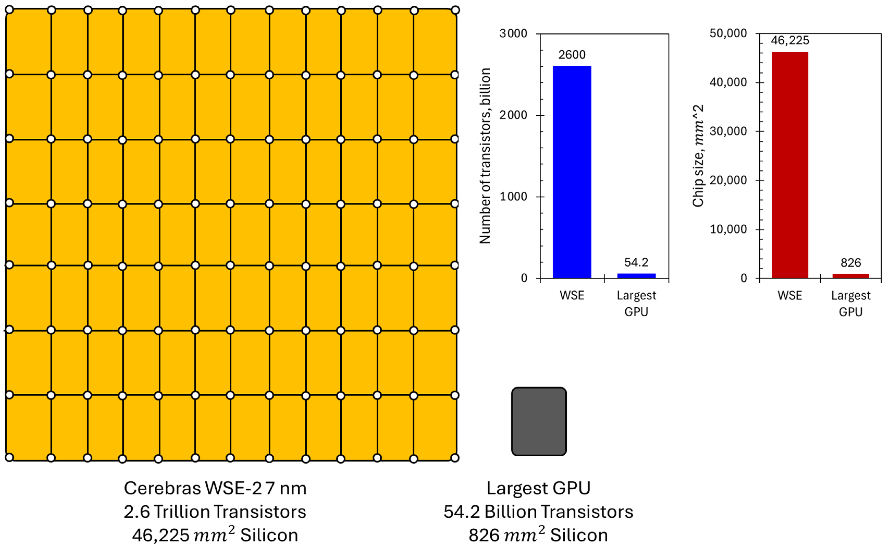
WSE CS-2, the WSE used in this study, integrates 850,000 compute cores (850 × 1000 array of tiles) over 462 cm2 of silicon area with 2.6 trillion transistors, 40 GB on-chip memory, 20 PB/s memory bandwidth, and 220 PB/s fabric bandwidth to enable highly efficient calculations [41]. The size of CS-2 is nearly 56 times the largest GPU size, NVIDIA A100 (Figure 2). The WSE comprises tiles, which are analogous to nodes on an HPC cluster. Each tile acts independently with its own program code or as a group for collective operations [41]. The entire WSE tiles form a 2D array, with local communication paths between each tile and its Cartesian neighbors. The integrated chip design makes WSE behave more like a single workstation than computer clusters. By significantly reducing I/O time, the WSE achieves unparalleled high efficiency in solving complex numerical models. WSE CS-3, the latest generation of WSE, features 900,000 AI-optimized cores, enabling even higher levels of parallelism for training large-scale models [42].
Unlike the extensive research that has already been conducted on full-physics and ML models for subsurface flow modeling using conventional computing hardware (CPU and GPU), wafer-scale computing is still at its nascent stage, requiring unconventional system design, compiler design, and domain-specific API. As a result, functionalities and algebraic solvers that are readily available in many CPU/GPU-based numerical libraries oftentimes need to be built from scratch. In the context of this study, so far, limited research has been conducted to benchmark the power of wafer-scale computing technology for reservoir simulations. The only study related to this work is Sai et al. [43], who presented a finite volume implementation for compressible single-phase flow, demonstrating the potential of WSE for improving full-physics simulation computational performance.
The literature review highlights a gap between high-fidelity full-physics solvers and fast but non-generalizable ML surrogates. Existing hardware advances, including GPUs, have improved scalability but remain limited by inter-node communication. Wafer-scale computing uniquely addresses this gap by combining physics robustness with real-time performance, motivating the present study to explore its feasibility for CO2-brine flow simulation.
This study develops a fully coupled, multiphase flow reservoir simulator using a newly developed in-house, WSE API, providing a systematic rigorous benchmarking of the developed solver. To the best of our knowledge, this is the first detailed case study aiming to elucidate the capability of wafer-scale computing for reservoir-scale multiphase simulations.

3. Methodology

This section outlines the methodology for developing and implementing a multiphase reservoir simulator. Building on our preliminary work [44] that examined the potential of WSE for large-scale reservoir simulations, the study expands the solver to handle two-phase compressible flows. A case study focused on CO2 injection into a saline aquifer at the Illinois Basin Decatur Project (IBDP) site was selected to demonstrate the model capabilities.

3.1. Physics-Based Mathematical Model

The developed simulator is formulated as a multiphase compressible flow model representing CO2 and brine interactions in deep saline aquifers. It incorporates the key physical mechanisms that govern carbon storage performance. These include representation of PVT properties of both phases, the dissolution of CO2 into brine, and buoyancy-driven plume migration resulting from the density contrast between CO2 and brine. Rock compressibility is also accounted for, ensuring that porosity changes induced by pressure variations are captured in the model. To provide a rigorous foundation, this section presents the governing partial differential equations (PDEs) for multiphase flow in porous media and outlines their numerical solution using the finite-difference method. The Peng–Robinson Equation of State (EOS) [5] is introduced to evaluate PVT properties of CO2 under reservoir conditions, while Corey’s model [6] is applied to characterize relative permeabilities of the coexisting phases. Together, these formulations establish a high-fidelity mathematical framework capable of simulating both fluid and rock responses relevant to geologic carbon storage. The flow is assumed to be isothermal.
The governing framework for the two-phase CO2-brine system is expressed through a coupled set of PDEs. These include the continuity equation, which enforces mass conservation for each phase: Darcy’s law, which describes fluid flow in porous media; and the EOS, which links pressure, temperature, and fluid properties. The generalized form of Darcy’s law was applied to account for multiphase flow conditions, ensuring that the formulation captured relative permeability effects and phase-dependent mobility. The governing expression for the brine phase is formulated as follows:
φ ρ w S w t = ρ w μ w k k r w p w + γ w z + q w ,
where φ is reservoir porosity, ρ w is brine density, S w is brine saturation, t is time, μ w and k r w are brine viscosity and relative permeability, k is absolute permeability, p w is brine pressure, γ w = ρ w g is brine gravity, and q w is brine injection/production source.
Parallel to the brine phase, the CO2 flow equation includes contributions from phase density, saturation, solubility of CO2 in brine, pressure gradients, gravitational forces, and external injection or production sources. These terms capture the dynamics of injected CO2 as it migrates through the porous media while interacting with the reservoir brine:
  φ   ρ g   S g +   ρ w   S w R s w t = · ρ g μ g k   k r g + ρ w μ w k   k r w R s w p g + γ g z   + q g ,
where ρ g , S g and R s w are CO2 density, CO2 saturation, and CO2 solubility in brine, p g is gas phase pressure, γ g = ρ g · g is gas phase gravity term, and q g is CO2 injection/production term. In multiphase flow, the phase saturation (e.g., S w and S g ) is defined as the fraction of pore volume that is occupied by a fluid (e.g., water, and gas) and can be represented as follows:
S w = V w V p ,
S g = V g V p ,
where V w and V g are the water and gas volumes, respectively, and V p is the total pore volume. It is worth noting that the saturation of each phase can range from 0 to 1, and the sum of saturations ( S w + S g ) is equal to 1 for a saturated medium.
To establish a unified formulation, the brine and CO2 phase equations are combined into an overall flow equation. This is achieved by multiplying the brine-governing expression (Equation (1)) by a weighting factor ( B w / B g R s w ) and adding it to the CO2 gas phase expression (Equation (2)), yielding a composite PDE that governs total flow in the system. Both the brine-phase PDE and the overall flow PDE are then discretized in space and time using the finite-difference method, enabling numerical solution. Equation (1) was discretized in time and in space, following the IMPES scheme (Implicit Pressure, Explicit Saturation). The fully discrete form for cell (i, j, k) is given by Equation (5a,b). Equation (5a,b) are formulated using the finite-difference method.
Multiplying each side of Equation (1) by cell volume V i j k = Δ x Δ y Δ z and discretizing in space and time gives a R.H.S as follows:
V i j k φ ρ w S w t = T w i + 1 2 , j , k P i + 1 , j , k P i , j , k + ( T w ) i 1 2 , j , k P i 1 , j , k P i , j , k + T w i , j + 1 2 , k P i , j + 1 , k P i , j , k + ( T w ) i , j 1 2 , k P i , j 1 , k P i , j , k + T w i , j , k + 1 2 P i , j , k + 1 P i , j , k + ( T w ) i , j , k 1 2 P i , j , k 1 P i , j , k + T w   γ w i , j , k + 1 2 z i , j , k + 1 z i , j , k + T w γ w i , j , k 1 2 z i , j , k 1 z i , j , k + V i j k   q w
where T w i + 1 2 = A Δ x i + 1 2 k   k r w B w μ w i + 1 2 .   ρ w = ρ w 0 B w 0 B w , where ρ w , and B w are water density and formation volume factor. ρ w 0 and B w 0 are estimated at reference conditions. The discretization of the L.H.S gives as follows:
V i j k φ ρ w S w t = V i j k Δ t φ S w B w n + 1 φ S w B w n = V i j k φ B w n + 1 Δ S w Δ t + V i j k S w Δ φ B w Δ t = V i j k φ B w n + 1 Δ S w Δ t + V i j k S W n Δ φ B w Δ t = V i j k φ B o n + 1 Δ S w Δ t +   V i j k S w n Δ t φ B w n + 1 φ B w n + B w n + 1 φ n B w n + 1 φ n = V i j k φ B o n + 1 Δ S w Δ t   +   V i j k   S w n 1 B w n + 1 Δ φ Δ t + φ n Δ 1 B w Δ t =   V i j k φ B o n + 1 Δ S w Δ t   +   V i j k   S w n 1 B w n + 1 Δ φ Δ P + φ n Δ 1 B w Δ P Δ P Δ t
where φ is reservoir porosity, ρ w is brine density, S w is brine saturation, t is time, n is current timestep, n + 1 is new timestep, μ w and k r w are brine viscosity and relative permeability, k is absolute permeability, p w is brine pressure, γ w = ρ w g is brine gravity, and q w is brine injection/production source. The second governing equation (Equation (2)) follows the same discretization schemes. Since the saturation is computed explicitly, a sufficiently small timestep is used to ensure stability, and in this study, a constant timestep of 1 day was applied over the five-year simulation period to maintain numerical stability.
An important distinction lies in the variable dependencies of these equations. The overall flow equation depends solely on pressure, whereas the brine-phase equation depends on both pressure and saturation. Consequently, the solution procedure follows a sequential approach: the overall flow PDE is first solved to determine reservoir pressure distribution, and this pressure field is subsequently applied within the brine equation to compute saturation. This stepwise coupling ensures stable numerical behavior and provides consistent tracking of multiphase interactions throughout the reservoir.
The thermodynamic behavior of CO2 under reservoir conditions is represented using the Peng–Robinson EOS. This cubic EOS provides a relationship among pressure, temperature, and molar volume, making it a widely adopted model for subsurface applications. In this formulation, the universal gas constant ( R ) is combined with parameters that are functions of CO2 critical properties and acentric factor. These parameters capture the non-ideal behavior of CO2 across the conditions encountered in deep saline aquifers. The Peng–Robinson EOS used for calculating PVT properties [5] can be expressed as follows:
p = R T V m b a α V m 2 + 2 b V m b 2 ,
where p is pressure, T is temperature, and V m is molar volume. R is the general gas constant. Parameters a , b , and α are functions of CO2 properties (critical conditions and specific gravity). The equation is often used to calculate the compressibility factor, which is then used to obtain the PVT properties. The analytical real-gas equations are applied to obtain CO2 density and formation volume factor (FVF). Formation volume factor (FVF) for the gas phase, defined as the ratio of gas volume at reservoir conditions to its volume at standard/surface conditions ( B g = Vres/Vstd), is used to convert between reservoir and surface volumes. The CO2 viscosity is based on Fenghour et al. correlation [45], as shown in Figure 3.
In this work implementation on the WSE, the estimated PVT solutions (Figure 3) are approximated using fourth-order polynomial functions. This approach optimizes memory usage and improves computational efficiency on the WSE, instead of solving Equation (6), which would require additional computational resources and memory. Nevertheless, the nonlinear Equation (6) can be solved when necessary. The model internally employs polynomial correlations for gas density, viscosity, and formation volume factor across the full operational pressure range used in the simulations. Figure 3 is included as an illustration of these relationships. In this study, the Peng–Robinson EOS (Equation (6)) was used to generate the CO2 property data that were then approximated by fourth-order polynomial correlations for use in the WSE solver. The solver itself directly employs these polynomial functions, while the EOS can be solved separately if more detailed PVT data are required.
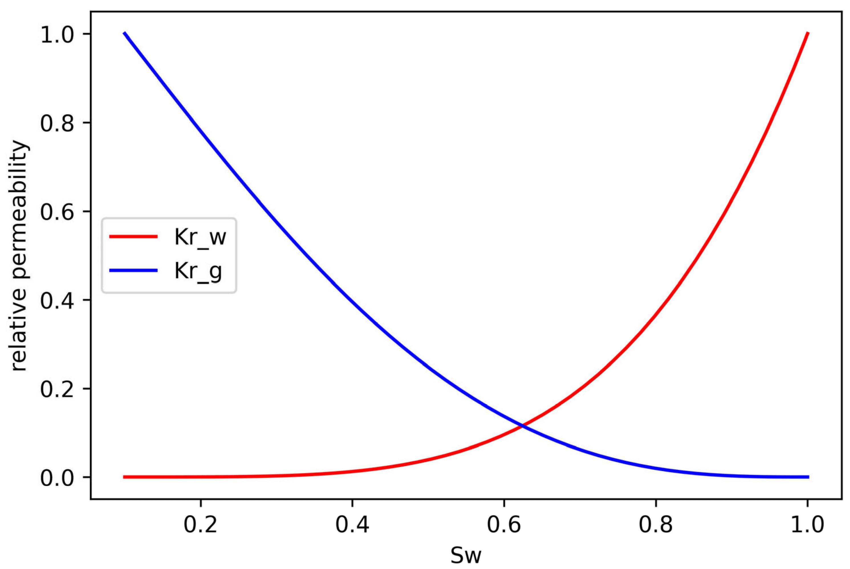
The relative permeability relationships for the brine and CO2 phases (Figure 4) are represented using Corey’s model [6]. This formulation expresses the effective mobility of each phase as a nonlinear function of water saturation, with irreducible water and gas saturations serving as input parameters. By incorporating these endpoint constraints, the model ensures that the relative permeabilities approach zero as saturations reach their residual limits, thereby preserving physical consistency [6]:
k r w = s b 4 ,
k r g = 1 s b 2 1 s b 2 ,
s b = S w S w i 1 S w i r S g i r ,
where k r w and k r g are brine and gas relative permeabilities, respectively, S w is water saturation, S w i is initial water saturation, and S w i r and S g i r are the irreducible water and gas saturations. Capillary pressure and three-phase flow are not included in this study, as the present work focuses on presenting the WSE computational performance for two-phase, CO2-brine systems. For a saturated medium, the pressure equation is first solved, followed by determination of water saturation using the relative permeability–saturation relationship. The governing equations are thus sequentially coupled through pressure and saturation, consistent with standard multiphase flow formulations.

3.2. Implementation on the WSE

The U.S. Department of Energy’s (DOE) National Energy Technology Laboratory (NETL), one of the earliest adopters of the wafer-scale computing, has recently developed a high-level API for the WSE, which is called the WSE Field-equation API, or WFA [41,46]. The WFA has been demonstrated on multiple computational fluid dynamics problems and applications, outperforming NETL’s supercomputer, Joule 2.0, by over two orders of magnitude in compute time [41].
WFA provides an easy-to-use NumPy-like interface for implementing PDE solvers, allowing researchers to perform efficient large-scale physics-based simulations by using high-level Python scripting (version 3.13.3) [40,46]. The wafer-scale computing of this study was performed on the Pittsburgh Supercomputing Center’s Neocortex, a Cerebras® CS-2 WSE [47]. Cerebras® is a startup company located in Sunnyvale, CA, USA. The Neocortex system is accessible and free-of-charge to the research community through proposal-based allocations.
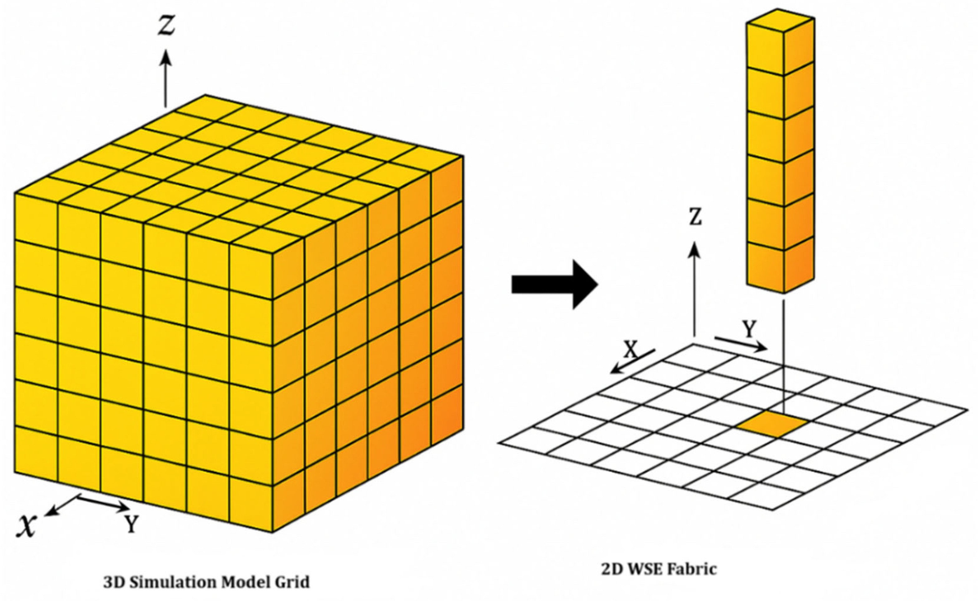
As mentioned in the Introduction, the data flow architecture of WSE is a 2D mesh interconnection fabric that connects PEs, as demonstrated in Figure 5. PEs are the units where actual computations occur. In a 3D simulation case, the domain is decomposed such that the simulation model cells in X- and Y-directions are mapped across the 2D WSE fabric. However, the cells in the Z-direction are mapped to the same PE. In other words, a simulation cell of coordinates (x, y, z) is mapped to the PE of coordinates (x, y) [43].
In a typical WSE application development cycle, the end user first develops a solver in Python, using the WFA classes and class decorators modifying the original NumPy classes. The NETL compiler is used to translate the Python code into an Intermediate Language, which is a language used internally by the compiler. An interface layer creates an Intermediate Representation Graph (IRG) from the Intermediate Language and, finally, a set of IRG-Interpreters (IRGIs) translate the IRG to various target languages, such as Tungsten, the high-level language used by the WSE to pass arguments between PEs [48].
For the two-phase flow problem being solved, application of the finite-difference scheme results in seven-diagonal sparse matrix systems. That is, for each cell in the 3D grid, only values from the north, south, east, west, top, and bottom adjacent cells enter the coefficient matrices. The sparse linear system of equations is solved using WFA’s BiCGStab solver, an implementation of the biconjugate gradient stabilized method [49]. The convergence tolerance is set to 10−6. The computational grid was mapped directly to the WSE cores using spatial decomposition. Each core handled a defined portion of the grid with local memory to minimize data exchange.
In our case, when solving nonlinear PDEs with the linear solver BiCGSTAB, the linear solver only handles a linearized subproblem (it only solves a linear system of A n *   P n + 1 = B n , where A n and B n are the coefficients based on the current timestep “n” data, such as pressure, updated porosity, and updated PVT for solving next timestep “n + 1” solution P n + 1   with coefficients “frozen” from the previous iteration timestep. However, the overall algorithm remains nonlinear because these coefficients and source terms depend on the evolving solution (such as pressure, porosity, and PVT). The process involves an outer nonlinear loop (where the system matrix and source are reassembled based on the updated solution) and an inner linear loop (where BicgSTAB solves the resulting linear system). This sequence, which solves the underlying nonlinear PDE through successive linear approximations, is repeated until the convergence or time-matching criteria are met.

3.3. Design of Benchmark Studies

The Python-based multiphase flow solver was first validated against analytical solutions corresponding to the Buckley–Leverett problem. Results, shown in Appendix A, suggest the solver satisfactorily captures the evolution of the saturation front. In addition, the developed solver was tested for three-dimensional numerical consistency, as presented in our earlier work that was presented as slides at the 2024 Carbon Management Research Project Review Meeting [44], which compared the accuracy of the solver against a commercial reservoir simulator. For this work, we selected GEOS® as the CPU baseline because it is a widely used open-source multiphase flow simulator, along with its availability on the NETL Joule 3 HPC system, providing a reproducible comparison against the WSE runs.
For the large-scale CO2 storage benchmarking, a 3D model representative of the Illinois Basin Decatur Project (IBDP) site was developed. IBDP was a joint effort between Schlumberger Carbon Services, the Illinois State Geological Society, and Archer Daniels Midland Company, along with multiple subcontractors [7]. The goal of IBDP was to demonstrate the safety and efficacy of a complete source-to-pipeline carbon capture and storage system. The IBDP began in 2007 with three phases that lasted about 13 years, including a pre-injection phase, injection phase, and post-injection phase. From 2011 to 2014, around 1 million metric tons of CO2 were injected into Mt. Simon Sandstone at a depth of 2072 m.
The original IBDP model covers a 15.5 km × 14.9 km footprint. The spatial domain is discretized by a 126 × 125 × 110 non-uniform structured grid, with the smallest grid size found near the injector (38.1m × 38.1 m) [8]. For proof-of-concept, this study considered an IBDP-like domain: the reservoir domain is 15 km × 15 km × 1 km and is discretized by a uniform 124 × 124 × 108 grid (Figure 6). A single cell at the center of the model domain is used for injecting CO2, at a constant rate of 10 kg/s for 5 years. The horizontal permeability is set to 100 mD (9.869 × 10⁻¹⁴ m2), while the vertical permeability is set to 10 mD. All model outer boundaries are set to closed boundaries. The initial pressure distribution is at hydrostatic pressure equilibrium. The simulation parameters are defined as follows: porosity = 0.20, temperature = 100 °C, residual water saturation = 0.10, and residual gas saturation = 0.0, as illustrated in Figure 4 for the relative permeability curves. The PVT properties for CO2 follow the correlations shown in Figure 3.
Performance of the WSE simulator is compared to the CPU-based GEOS, which uses message passing interface (MPI) distributed-memory for parallelization. For this study, all GEOS runs were conducted on NETL’s Joule 3 supercomputer. Each CPU-node on Joule 3.0 features two AMD® EPYC 9534 processors (64-core) and 384 GB of RAM. The CPU nodes are connected via Nvidia® NDR200 Infiniband (200 Gbps) cables. The AMD EPYC 9534 processor is manufactured by Advanced Micro Devices, Inc. (AMD), a U.S.-based semiconductor company. Nvidia® is a U.S. technology firm based in Santa Clara, CA, USA. For performance benchmarking, the same IBDP-like, GEOS model was run multiple times, using an increasing number of CPU cores.

4. Results and Performance Analysis

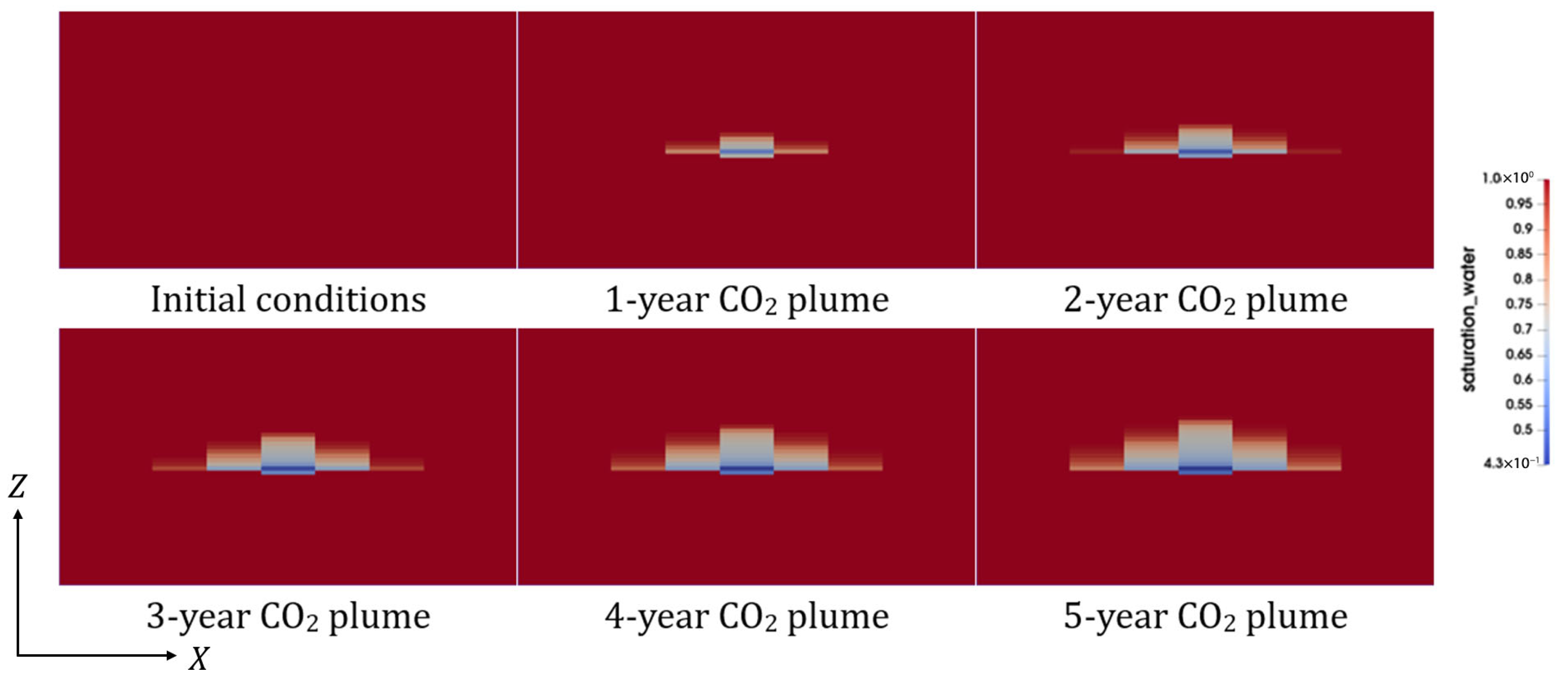
The CO2 plume evolution simulated by the WSE reservoir simulator is shown in Figure 7, which highlights the control of reservoir anisotropy on flow dynamics. With horizontal permeabilities of 100 mD in the x- and y-directions and a vertical permeability of only 10 mD, the resulting 10:1 anisotropy ratio restricts upward migration. This anisotropy not only dictates plume geometry but also provides a realistic stress test for the simulator by forcing it to capture the competing effects of buoyancy and permeability barriers. Starting from a brine-saturated reservoir, CO2 injection generates a plume centered at the injection point after the first year, with buoyancy-driven migration dominating the initial dynamics due to the density contrast between CO2 and brine. As injection continues, lateral spreading becomes increasingly significant, while vertical rise is limited by the permeability anisotropy. By the third year, the plume exhibits a combined pattern of modest upward migration and broad lateral expansion, and in years 4 and 5, the lateral expansion continues to grow while vertical movement remains constrained. The rectangular patterns in Figure 7 largely result from the uniform Cartesian mesh (124 × 124 × 108) and homogeneous properties used in the simulation. Capillary pressure was not included in this case, which explains the sharper saturation transitions observed.
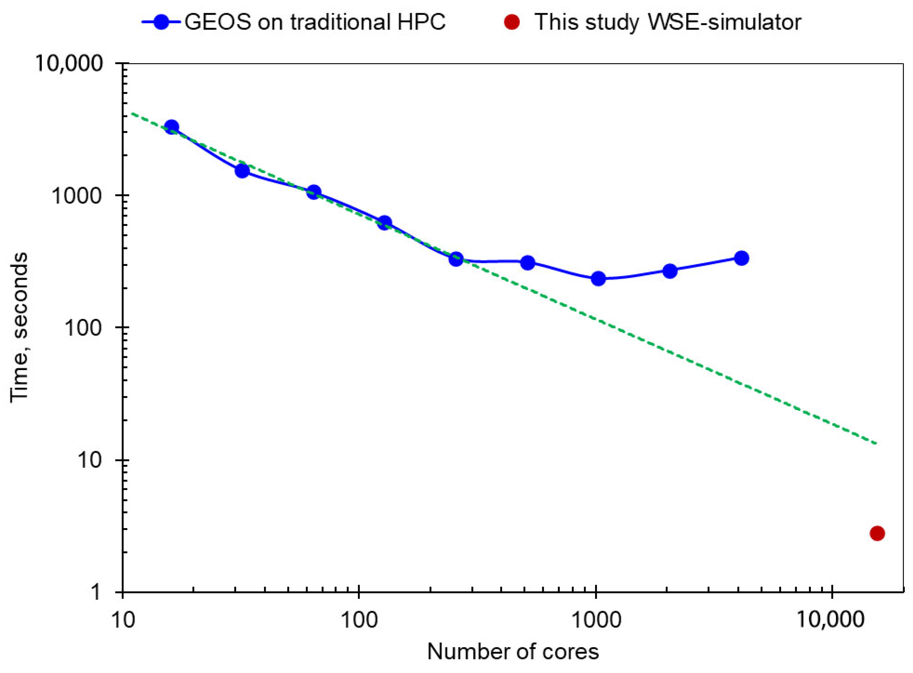
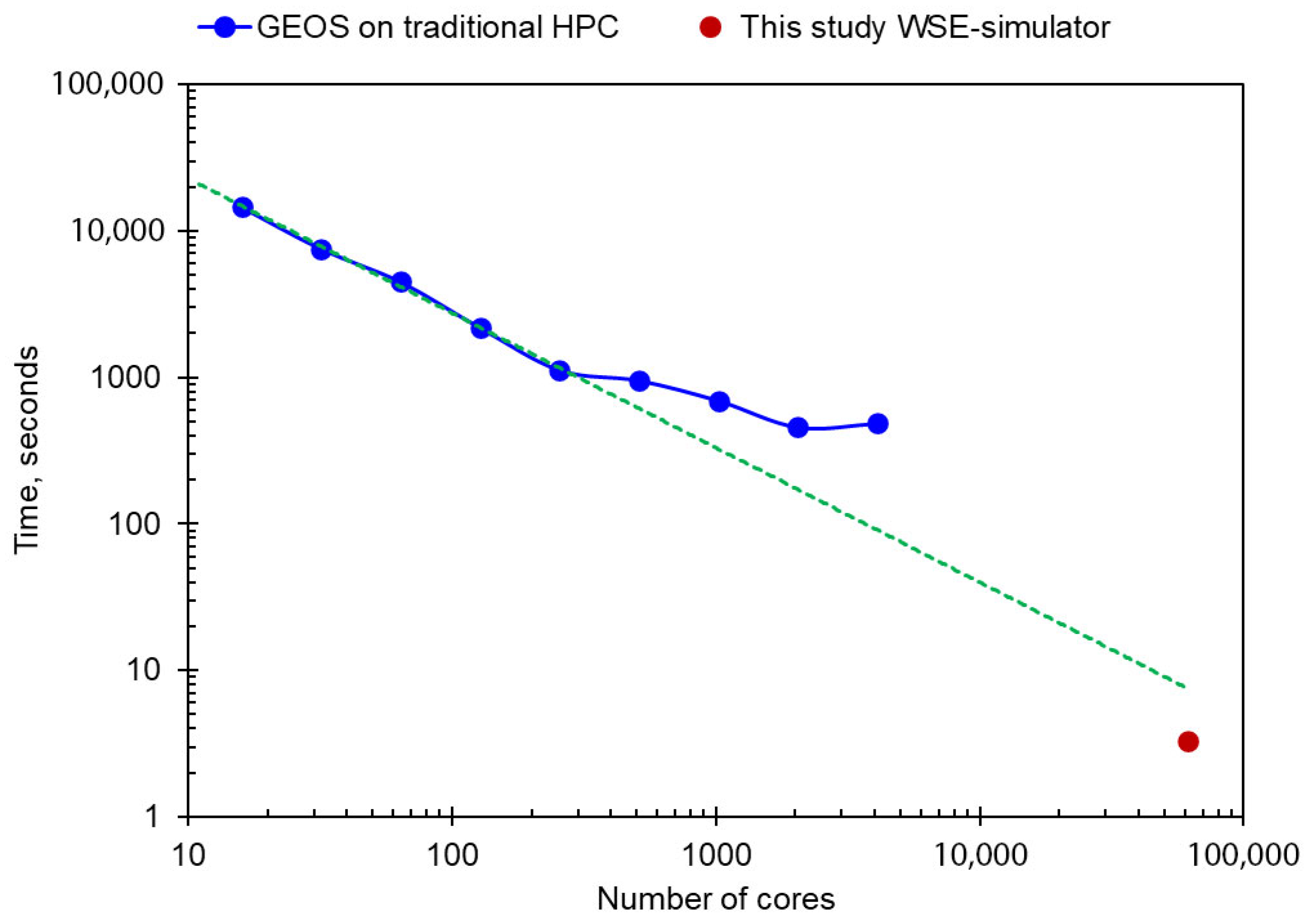
The computational times of GEOS and WSE are compared in Figure 8 on a log–log plot. The GEOS simulator, running on an HPC (NETL’s Joule 3.0 cluster), shows improved performance as the number of CPUs increases, but the benefit from additional CPUs reaches a plateau at 256 cores with a total simulation time of 334 s, because of the increasing inter-node communications and I/O bandwidth limitations. In comparison, the WSE simulator performs the same simulation in 2.82 s, representing a 118-fold speedup compared to the best performance from GEOS (see Table 1). The WSE solver used only 15,376 compute cores (124 in x-direction and 124 in y-direction), which is a small fraction (~1.8%) of the total 850,000 cores available on WSE CS-2. Thus, the WSE multiphase flow solver has shown a superior performance boost as compared to its CPU counterpart, and its speed can be further improved when more WSE compute cores are used.
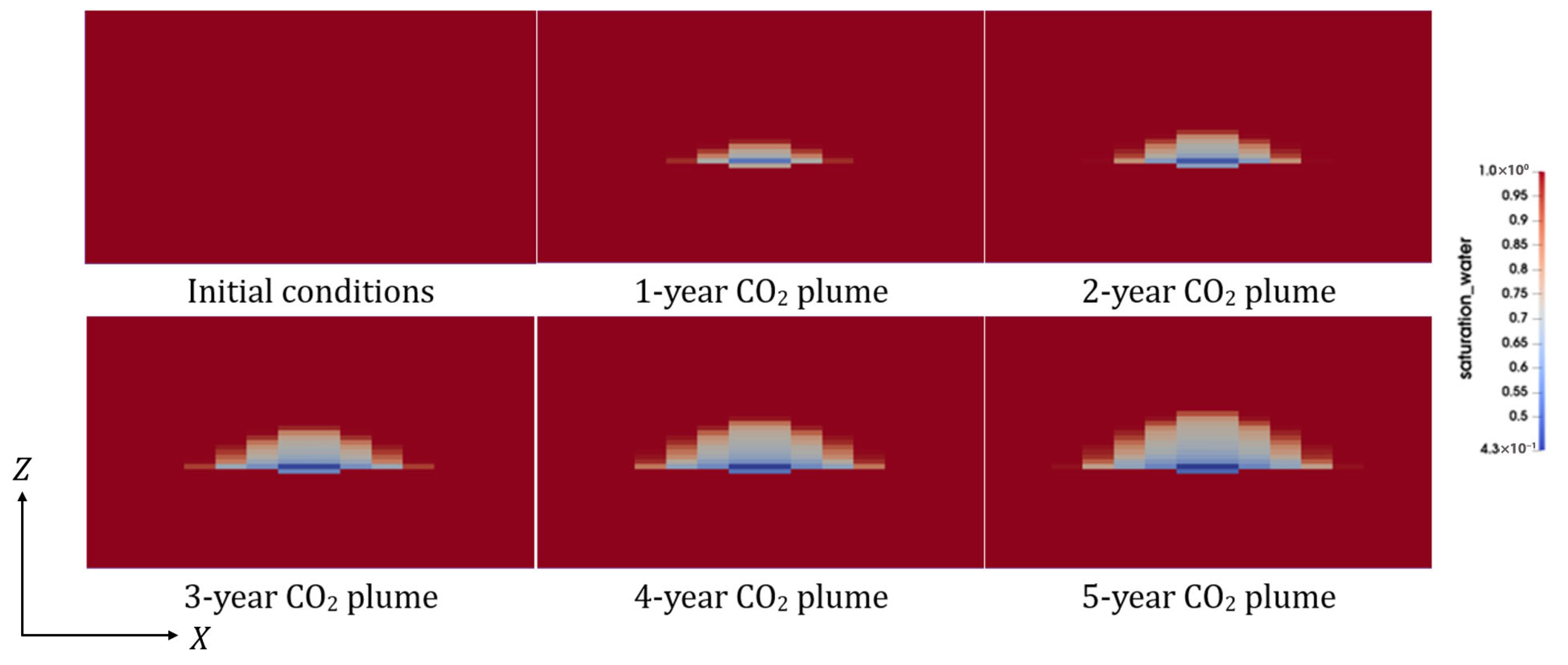
To evaluate scaling behavior under increased resolution, the simulation mesh was refined by doubling the grid counts in the x- and y-directions (from 124 × 124 to 248 × 248), while keeping the vertical discretization unchanged. This refinement increases the total number of cells by a factor of four, yielding 6.64 million active cells (Table 1). The refined mesh improves spatial resolution in the horizontal plane, allowing a more detailed capture of plume spreading. The higher resolution produces smoother plume structures and reveals finer-scale features in the evolving CO2 geometry (Figure 9), particularly in the lateral extent of the plume front. The simulation in Figure 9 was performed using a finer mesh compared to Figure 7 to examine resolution effects. The results demonstrate stable numerical performance and consistent plume geometry, while the main objective of this work remains to demonstrate the simulator computational performance on the WSE.
Importantly, despite this substantial increase in computational load, the developed WSE simulator completed the refined case in just 3.28 s, only a 16% increase over the base case runtime (Figure 10). By contrast, GEOS plateaued at 256 cores and required 1123 s, representing a 236% increase relative to its base case. This difference highlights the advantage of wafer-scale computing: runtime is nearly insensitive to grid refinement, enabling large-scale high-resolution studies without incurring the steep performance penalties observed in conventional HPC solvers. Such behavior suggests that the WSE paradigm can support model refinement, a critical requirement for uncertainty quantification and decision support in field applications. Runtime remained nearly unchanged between the base grid and the refined grid used here, indicating favorable scaling on the WSE for the cases tested. In Figure 10, the GEOS runtime continues to decrease beyond 256 cores, but with reduced efficiency as communication overhead begins to appear. The 256-core case was chosen for comparison because it represents a balanced point before this effect becomes noticeable.

5. Discussion

In practical terms, the demonstrated speed and fidelity of the WSE-based simulator implies that near-real-time, high-resolution, full-physics reservoir simulations may become feasible, and may be integrated into real-time decision-making workflows. As a result, field practitioners can run multiple high-fidelity scenarios in seconds, significantly enhancing both the speed and quality of operational decisions.
Table 2 summarizes the advantages and limitations of the proposed WSE technology in comparison to the ML and full-physics approaches. On one hand, the traditional full-physics models are known for their accuracy due to direct numerical solutions to the governing PDEs; however, they are computationally expensive and require long runtimes. On the other hand, the ML simulators are fast but are limited by training data requirements and a reduced generalizability. The proposed WSE-based simulator offers the high computational speed of the ML models and the accuracy characteristic of the traditional full-physics models. Compared to GEOS on the traditional HPC hardware, the developed WSE simulator accomplished the large-scale simulation cases in a few seconds, achieving speedups of over two orders of magnitude. This balance of speed, accuracy, and generalizability establishes the WSE-based simulator as a pivotal advancement for the large-scale subsurface flow modeling. Because wafer-scale computing is at an early stage, migrating a legacy simulator to the WSE still requires significant work, including rewriting the code to take advantage of the wafer parallelism. With time, the learning curve is expected to decrease as the WSE API is being continuously improved [48].
As a proof-of-concept, this work mainly focused on homogeneous formation properties. Inclusion of heterogeneous formation properties in the solver is straightforward and will be investigated in the future.
While the WSE reservoir simulator developed in this study is applied to geological carbon storage, the simulator and related workflow can be adapted to a wide range of subsurface energy applications, including enhanced oil recovery, hydrogen and natural gas storage, produced water disposal, water flooding, and gas injection for oil reservoirs. The continuous evolution of the NETL WFA would make the multiphase flow application development easier for future broad applied energy applications.
Equipment cost is constantly changing and difficult to compare. In a recent study using the same WSE CS-2 hardware, Woo et al. [41] compared FLOPS and energy consumption. At the largest fabric sizes tested in their study (750 × 950 mm2), they reported that WSE consumed an average of 24.6 kW, which is equivalent to about 32 to 35 gigaflops per watt. They concluded that the WFA (on WSE) is more than two orders of magnitude more energy-efficient than distributed computing.
Advances in gas storage extend beyond simulation efforts to include material innovations such as adsorbent carbon fiber composites developed for methane storage [50], which highlights complementary directions in achieving efficient gas management through both material design and computational modeling.
The WSE-based simulator can also complement machine learning workflows by rapidly generating high-fidelity datasets for surrogate model training. This capability enables hybrid approaches that combine physical accuracy with ML efficiency. While the current study focuses on demonstrating WSE performance and validation on a representative case, further testing across multiple geological scenarios will be pursued to confirm broader applicability. The presented framework establishes the foundation for extending WSE-based simulation to more complex and heterogeneous geological settings. Implementation aspects, including domain mapping and computational structure, have been clarified. As mentioned earlier, the WSE solver development is still at a nascent stage. The future will depend on the adoption rate of the WSE hardware itself, and the maturity level of WFA. If we reach that stage, it may be possible to replace the traditional ML surrogate models with WSE solvers.
The verification in this study was performed analytically to confirm the accuracy of the WSE implementation. The focus was to demonstrate the performance of WSE for two-phase flow simulations. Heterogeneous permeability cases are planned for future work.
The present tests used homogeneous models for verification. The same framework can also simulate heterogeneous formations and be extended to three-phase flow and different geological basins, as the wafer-scale solver maps directly to any grid and physics setup.

6. Conclusions

Wafer-scale computing is a new computing paradigm that can fundamentally change the landscape of scientific computing and machine learning. This study presented the development of a multiphase compressible flow reservoir simulator using the WSE. The model incorporates detailed physics, including Peng–Robinson EOS, Corey’s relative permeability, CO2 solubility in brine, buoyancy segregation due to CO2-brine density contrast, and pressure-dependent porosity. It was validated against the classical Buckley–Leverett analytical solution, showing agreement and confirming the simulator accuracy.
To assess the performance, 3D cases were simulated using both the developed WSE-based simulator and GEOS, which is a CPU-based parallel solver. The results showed that GEOS plateaued in performance around 256 CPU cores; however, the WSE completed the same simulation in just a few seconds using a small fraction of its full capacity, achieving more than two orders of magnitude speedup. This gain in computational performance is attributed to the WSE hardware architecture that eliminates the expensive internodal data transfer. This work showed that the WSE-based model can perform rapid and accurate full-physics reservoir simulations. This unique integration of accuracy and efficiency establishes a new superior paradigm for reservoir simulation, advancing both scientific research and practical decision-making in carbon storage and related subsurface energy applications.

Author Contributions

Conceptualization, M.K., H.K., A.Y.S., D.V.E., C.Y.S., G.L. and H.S.; methodology, M.K., H.K. and A.Y.S.; software, M.K., H.K., A.Y.S. and D.V.E.; validation, M.K., H.K. and A.Y.S.; formal analysis, M.K., H.K. and A.Y.S.; investigation, M.K., H.K. and A.Y.S.; resources, M.K., H.K., A.Y.S., D.V.E. and C.Y.S.; data curation, M.K., H.K. and A.Y.S.; writing—original draft preparation, M.K. and A.Y.S.; writing—review and editing, M.K., H.K., A.Y.S., D.V.E., C.Y.S., G.L. and H.S.; visualization, M.K., H.K. and A.Y.S.; supervision, H.S. All authors have read and agreed to the published version of the manuscript.

Funding

This research was supported by the U.S. Department of Energy’s (DOE) Office of Fossil Energy and Carbon Management project—the Science-informed Machine Learning for Accelerating Real-Time Decisions in Subsurface Applications (SMART) Initiative.

Data Availability Statement

The original contributions presented in this study are included in the article. Further inquiries can be directed to the corresponding author.

Acknowledgments

The authors are grateful to Joshua White and Chaoyi Wang at Lawrence Livermore National Laboratory for GEOS related discussion. This work used Neocortex at Pittsburgh Supercomputing Center through allocation ees220017p from the Advanced Cyberinfrastructure Coordination Ecosystem: Services & Support (ACCESS) program, which is supported by U.S. National Science Foundation grants #2138259, #2138286, #2138307, #2137603, and #2138296. This project was funded by the United States Department of Energy, National Energy Technology Laboratory, in part, through a site support contract. Neither the United States Government nor any agency thereof, nor any of their employees, nor the support contractor, nor any of their employees, makes any warranty, express or implied, or assumes any legal liability or responsibility for the accuracy, completeness, or usefulness of any information, apparatus, product, or process disclosed, or represents that its use would not infringe privately owned rights. Reference herein to any specific commercial product, process, or service by trade name, trademark, manufacturer, or otherwise does not necessarily constitute or imply its endorsement, recommendation, or favoring by the United States Government or any agency thereof. The views and opinions of authors expressed herein do not necessarily state or reflect those of the United States Government or any agency thereof.

Conflicts of Interest

The authors declare no conflicts of interest.

Appendix A. Model Validation

This section discusses the analytical validation of the subsurface fluid dynamics simulation model developed in this study using the benchmark case study presented in the GEOS documentation [51]. The study presented here uses the same setup to ensure the reliability of the results. This case study is also used in the open-source multiphase flow simulator GEOS®, the CPU-solver used in the benchmarking studies, and for modeling CO2 core flood experiment [52]. This case is solved to obtain the temporal and spatial development of CO2 gas saturation along the core domain and verified against the Buckley–Leverett analytical solutions [53]. The one-dimensional linear flow is horizontal in a homogeneous and isotropic porous core (Figure A1). Initially, the experimental core is fully saturated with brine. Supercritical CO2 is then injected into the core inlet, while fluid is withdrawn from the core outlet. The fluid phases are assumed incompressible, and the capillary pressure and gravity effects are neglected.
The core flooding with supercritical CO2 introduces an advancing saturation front, forming a sharp leading edge and advances across the core with time. The shock front saturation is found using tangent construction on the fractional flow curve. Here, the fractional flow of a phase (e.g., water) is the fraction of total flow rate that represents the phase in the two-phase flow system. The fractional flow function is derived from Darcy’s law and relative permeabilities. In this work, the power–law Brooks–Corey relation is used to define the gas and water relative permeabilities as follows
k r g = k r g 0 S g * n g ,
k r w = k r w 0 S w * n w ,
where k r g 0 and k r w 0 are the maximum relative permeability of gas and water phase, respectively; n g and n w are the Corey exponents; the dimensionless volume fraction (saturation) of gas phase, S g * , and water phase, S w * , are given as
S g * = S g S g r 1 S g r S w r ,
S w * = S w S w r 1 S g r S w r .
The fractional flow function of the gas phase ( f g ) as given by the Buckley–Leverett theory with constant fluid viscosities ( μ g and μ w ) can be described as
f g = k r g / μ g k r g / μ g + k r w / μ w .
The distribution of gas saturation as a function of distance and time is described as
x S g = Q T t A ϕ f g S g ,
where x S g is distance of saturation S g , Q T is injection rate, t is time, A is cross-sectional area, ϕ is reservoir porosity, and f g / S g is the fractional flow derivative with respect to S g . To derive results in dimensionless form, the dimensionless time t and dimensionless distance x d can be described as
t = Q T t A D L ϕ ,
x d = x S g D L .
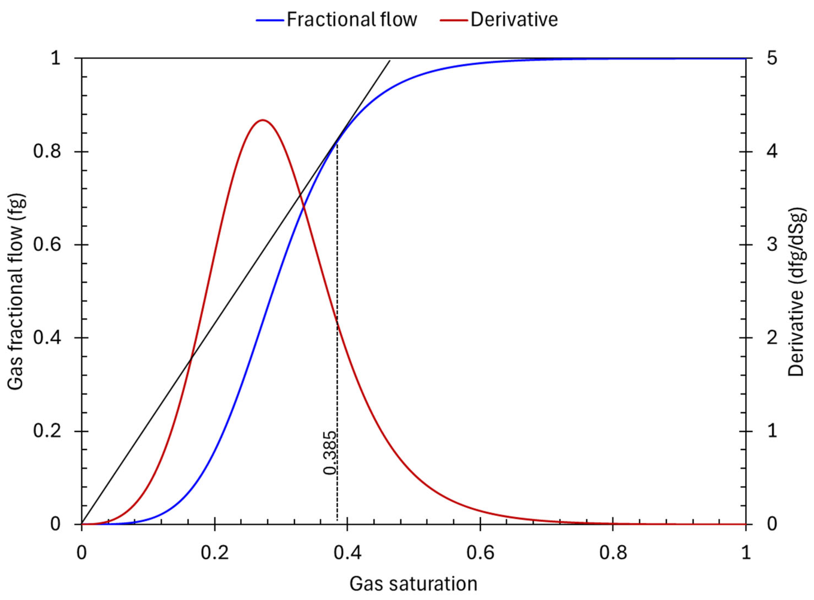
Table A1 lists the inputs used to validate the numerical model, including fluid viscosities, relative permeability parameters, and saturation endpoints. The domain dimensions used in the Buckley–Leverett simulation are illustrated in Figure A1. The fractional flow curve and its derivative constructed using the input parameters are presented in Figure A2. The fractional flow curve captures the nonlinear relationship between saturation and the fractional flow. The tangent/derivative to the curve from the initial saturation conditions determine the shock front saturation, which is an input in deriving the saturation profiles.
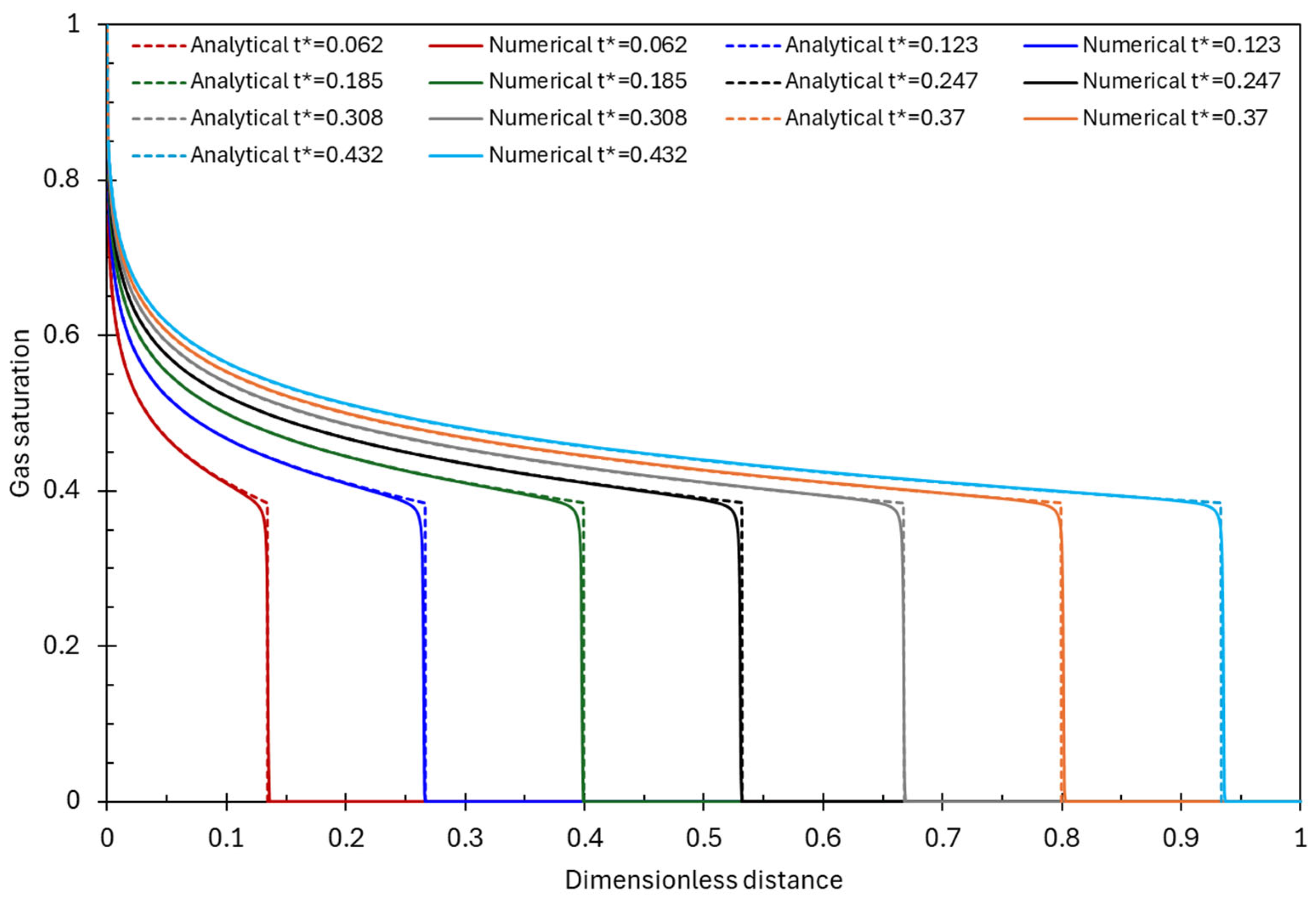
In Figure A3, the numerical results are shown along with the analytical Buckley–Leverett results at several dimensionless times, ranging from 0.062 to 0.432. The results comparison exhibits a good match across all the examined dimensionless times, with the saturation fronts aligning accurately, demonstrating the numerical model accuracy of the developed flow solver.
Table A1. Model input parameters.
ParameterValue
Max. Relative Permeability of Gas k r g 0 1.0
Max. Relative Permeability of Water k r w 0 1.0
Corey Exponent of Gas n g 3.5
Corey Exponent of Water n w 3.5
Porosity ϕ 0.2
Matrix Permeability k 9.0 × 10⁻¹³ m2
Gas Viscosity μ g 2.3 × 10⁻⁵ Pa s
Water Viscosity μ w 5.5 × 10⁻⁴ Pa s
Total Flow Rate Q T 2.5 × 10⁻⁷ m3/s
Domain Length D L 0.1 m
Domain Width D w 1.0 m
Domain Thickness D T 0.002 m
Figure A1. Schematic illustration of the model domain.
Energies 18 05874 g0a1
Figure A2. Fractional flow curves of CO2-brine flood experiment for model validation. The black solid line is the tangent, and the black vertical dashed line marks the associated saturation point.
Energies 18 05874 g0a2
Figure A3. Comparison of results from the numerical model developed in this study to Buckley–Leverett analytical solution. t* is dimensionless time.
Energies 18 05874 g0a3

References

  1. Wang, Y.; Jin, Y.; Pang, H.; Lin, B. Upscaling for Full-Physics Models of CO2 Injection Into Saline Aquifers. SPE J. 2025, 30, 3065–3082. [Google Scholar] [CrossRef]
  2. Khalaf, M.; Liu, G.; Dilmore, R.; Lackey, G.; Mehana, M.; Cunha, L.; Strazisar, B. Reservoir Dynamics in Proposed Operational Scenarios Where CO2-EOR Fields Are Transitioned From CO2-Flood Enhanced Oil Recovery to Dedicated Carbon Storage: A Field Case Study; US DOE National Energy Technology Laboratory: Pittsburgh, PA, USA, 2025. [Google Scholar] [CrossRef]
  3. Sun, A.Y. Optimal Carbon Storage Reservoir Management through Deep Reinforcement Learning. Appl. Energy 2020, 278, 115660. [Google Scholar] [CrossRef]
  4. Du, H.; Zhao, Z.; Cheng, H.; Yan, J.; He, Q. Modeling Density-Driven Flow in Porous Media by Physics-Informed Neural Networks for CO2 Sequestration. Comput. Geotech. 2023, 159, 105433. [Google Scholar] [CrossRef]
  5. Peng, D.-Y.; Robinson, D.B. A New Two-Constant Equation of State. Ind. Eng. Chem. Fundam. 1976, 15, 59–64. [Google Scholar] [CrossRef]
  6. Corey, A.T. The Interrelation between Gas and Oil Relative Permeability. Prod. Mon. 1954, 19, 38–41. [Google Scholar]
  7. Bauer, R.A.; Will, R.; Greenberg, S.E.; Whittaker, S.G. Illinois Basin–Decatur Project. In Geophysics and Geosequestration; Cambridge University Press: Cambridge, UK, 2019; pp. 339–370. [Google Scholar]
  8. DataShare, C. Illinois Basin—Decatur Project Dataset. Available online: https://co2datashare.org/dataset/illinois-basin-decatur-project-dataset (accessed on 15 September 2025).
  9. Koo, C.; Park, S.; Hong, T.; Park, H.S. An Estimation Model for the Heating and Cooling Demand of a Residential Building with a Different Envelope Design Using the Finite Element Method. Appl. Energy 2014, 115, 205–215. [Google Scholar] [CrossRef]
  10. Harish, V.S.K.V.; Kumar, A. Reduced Order Modeling and Parameter Identification of a Building Energy System Model through an Optimization Routine. Appl. Energy 2016, 162, 1010–1023. [Google Scholar] [CrossRef]
  11. Sun, Q.; Teng, R.; Li, H.; Xin, Y.; Ma, H.; Zhao, T.; Chen, Q. Generalized Frequency-Domain Analysis for Dynamic Simulation and Comprehensive Regulation of Integrated Electric and Heating System. Appl. Energy 2024, 372, 123817. [Google Scholar] [CrossRef]
  12. Service, R.F. Exascale Computers Show off Emerging Science. Science 2023, 382, 864–865. [Google Scholar] [CrossRef]
  13. Peherstorfer, B.; Willcox, K. Dynamic Data-Driven Reduced-Order Models. Comput. Methods Appl. Mech. Eng. 2015, 291, 21–41. [Google Scholar] [CrossRef]
  14. Lucia, D.J.; Beran, P.S.; Silva, W.A. Reduced-Order Modeling: New Approaches for Computational Physics. Prog. Aerosp. Sci. 2004, 40, 51–117. [Google Scholar] [CrossRef]
  15. Trifonov, V.; Illarionov, E.; Voskresenskii, A.; Petrosyants, M.; Katterbauer, K. Hybrid Solver with Deep Learning for Transport Problem in Porous Media. Discov. Geosci. 2025, 3, 33. [Google Scholar] [CrossRef]
  16. Chen, Z.; Zhao, X.; Zhu, H.; Tang, Z.; Zhao, X.; Zhang, F.; Sepehrnoori, K. Engineering Factor Analysis and Intelligent Prediction of CO2 Storage Parameters in Shale Gas Reservoirs Based on Deep Learning. Appl. Energy 2025, 377, 124642. [Google Scholar] [CrossRef]
  17. Zhang, Y.-F.; Qu, M.-L.; Yang, J.-P.; Foroughi, S.; Niu, B.; Yu, Z.-T.; Gao, X.; Blunt, M.J.; Lin, Q. Prediction of CO2 Storage Efficiency and Its Uncertainty Using Deep-Convolutional GANs and Pore Network Modelling. Appl. Energy 2025, 381, 125142. [Google Scholar] [CrossRef]
  18. San, O.; Maulik, R. Extreme Learning Machine for Reduced Order Modeling of Turbulent Geophysical Flows. Phys. Rev. E 2018, 97, 042322. [Google Scholar] [CrossRef]
  19. Luo, Z.; Wang, L.; Xu, J.; Wang, Z.; Yuan, J.; Tan, A.C.C. A Reduced Order Modeling-Based Machine Learning Approach for Wind Turbine Wake Flow Estimation from Sparse Sensor Measurements. Energy 2024, 294, 130772. [Google Scholar] [CrossRef]
  20. Zhong, Z.; Sun, A.Y.; Jeong, H. Predicting CO2 Plume Migration in Heterogeneous Formations Using Conditional Deep Convolutional Generative Adversarial Network. Water Resour. Res. 2019, 55, 5830–5851. [Google Scholar] [CrossRef]
  21. Mo, S.; Zabaras, N.; Shi, X.; Wu, J. Deep Autoregressive Neural Networks for High--Dimensional Inverse Problems in Groundwater Contaminant Source Identification. Water Resour. Res. 2019, 55, 3856–3881. [Google Scholar] [CrossRef]
  22. Tang, M.; Liu, Y.; Durlofsky, L.J. A Deep-Learning-Based Surrogate Model for Data Assimilation in Dynamic Subsurface Flow Problems. J. Comput. Phys. 2020, 413, 109456. [Google Scholar] [CrossRef]
  23. Wen, G.; Li, Z.; Azizzadenesheli, K.; Anandkumar, A.; Benson, S.M. U-FNO—An Enhanced Fourier Neural Operator-Based Deep-Learning Model for Multiphase Flow. Adv. Water Resour. 2022, 163, 104180. [Google Scholar] [CrossRef]
  24. Jin, Z.L.; Liu, Y.; Durlofsky, L.J. Deep-Learning-Based Surrogate Model for Reservoir Simulation with Time-Varying Well Controls. J. Pet. Sci. Eng. 2020, 192, 107273. [Google Scholar] [CrossRef]
  25. Sun, A.Y.; Yoon, H.; Shih, C.-Y.; Zhong, Z. Applications of Physics-Informed Scientific Machine Learning in Subsurface Science: A Survey. In Knowledge-Guided Machine Learning; Chapman and Hall/CRC: Boca Raton, FL, USA, 2022; pp. 111–132. [Google Scholar]
  26. Yanchun, L.; Deli, J.; Suling, W.; Ruyi, Q.; Meixia, Q.; He, L. Surrogate Model for Reservoir Performance Prediction with Time-Varying Well Control Based on Depth Generative Network. Pet. Explor. Dev. 2024, 51, 1287–1300. [Google Scholar] [CrossRef]
  27. Vo Thanh, H.; Yasin, Q.; Al-Mudhafar, W.J.; Lee, K.K. Knowledge-Based Machine Learning Techniques for Accurate Prediction of CO2 Storage Performance in Underground Saline Aquifers. Appl. Energy 2022, 314, 118985. [Google Scholar] [CrossRef]
  28. Etienam, C.; Juntao, Y.; Said, I.; Ovcharenko, O.; Tangsali, K.; Dimitrov, P.; Hester, K. A Novel A.I Enhanced Reservoir Characterization with a Combined Mixture of Experts—NVIDIA Modulus Based Physics Informed Neural Operator Forward Model. arXiv 2024, arXiv:2404.14447. [Google Scholar]
  29. Pachalieva, A.; O’Malley, D.; Harp, D.R.; Viswanathan, H. Physics-Informed Machine Learning with Differentiable Programming for Heterogeneous Underground Reservoir Pressure Management. Sci. Rep. 2022, 12, 18734. [Google Scholar] [CrossRef]
  30. Illarionov, E.; Temirchev, P.; Voloskov, D.; Kostoev, R.; Simonov, M.; Pissarenko, D.; Orlov, D.; Koroteev, D. End-to-End Neural Network Approach to 3D Reservoir Simulation and Adaptation. J. Pet. Sci. Eng. 2022, 208, 109332. [Google Scholar] [CrossRef]
  31. Zhou, K.; Liu, Z.; Qiao, Y.; Xiang, T.; Loy, C.C. Domain Generalization: A Survey. IEEE Trans. Pattern Anal. Mach. Intell. 2022, 45, 4396–4415. [Google Scholar] [CrossRef]
  32. Goswami, S.; Kontolati, K.; Shields, M.D.; Karniadakis, G.E. Deep Transfer Operator Learning for Partial Differential Equations under Conditional Shift. Nat. Mach. Intell. 2022, 4, 1155–1164. [Google Scholar] [CrossRef]
  33. Karniadakis, G.E.; Kevrekidis, I.G.; Lu, L.; Perdikaris, P.; Wang, S.; Yang, L. Physics-Informed Machine Learning. Nat. Rev. Phys. 2021, 3, 422–440. [Google Scholar] [CrossRef]
  34. He, X.; Zhu, W.; Kwak, H.; Yousef, A.; Hoteit, H. Deep Learning-Assisted Bayesian Framework for Real-Time CO2 Leakage Locating at Geologic Sequestration Sites. J. Clean. Prod. 2024, 448, 141484. [Google Scholar] [CrossRef]
  35. Wang, H.; Zhang, M.; Xia, X.; Tian, Z.; Qin, X.; Cai, J. Lattice Boltzmann Prediction of CO2 and CH4 Competitive Adsorption in Shale Porous Media Accelerated by Machine Learning for CO2 Sequestration and Enhanced CH4 Recovery. Appl. Energy 2024, 370, 123638. [Google Scholar] [CrossRef]
  36. Mack, C.A. Fifty Years of Moore’s Law. IEEE Trans. Semicond. Manuf. 2011, 24, 202–207. [Google Scholar] [CrossRef]
  37. Theis, T.N.; Wong, H.-S.P. The End of Moore’s Law: A New Beginning for Information Technology. Comput. Sci. Eng. 2017, 19, 41–50. [Google Scholar] [CrossRef]
  38. Hu, Y.; Lin, X.; Wang, H.; He, Z.; Yu, X.; Zhang, J.; Yang, Q.; Xu, Z.; Guan, S.; Fang, J.; et al. Wafer-Scale Computing: Advancements, Challenges, and Future Perspectives [Feature]. IEEE Circuits Syst. Mag. 2024, 24, 52–81. [Google Scholar] [CrossRef]
  39. Lauterbach, G. The Path to Successful Wafer-Scale Integration: The Cerebras Story. IEEE Micro 2021, 41, 52–57. [Google Scholar] [CrossRef]
  40. Van Essendelft, D.; Almolyki, H.; Shi, W.; Jordan, T.; Wang, M.-Y.; Saidi, W.A. Record Acceleration of the Two-Dimensional Ising Model Using High-Performance Wafer Scale Engine. arXiv 2024, arXiv:2404.16990. [Google Scholar] [CrossRef]
  41. Woo, M.; Jordan, T.; Schreiber, R.; Sharapov, I.; Muhammad, S.; Koneru, A.; James, M.; Van Essendelft, D. Disruptive Changes in Field Equation Modeling: A Simple Interface for Wafer Scale Engines. arXiv 2022, arXiv:2209.13768. [Google Scholar] [CrossRef]
  42. Hock, A. Accelerating AI and HPC for Science at Wafer-Scale with Cerebras Systems. In Proceedings of the Argonne Training Program on Extreme-Scale Computing (ATPESC); 2022. Available online: https://extremecomputingtraining.anl.gov/wp-content/uploads/sites/96/2022/11/ATPESC-2022-Track-1-Talk-8-Hock-Cerebras-for-ATPESC.pdf (accessed on 15 September 2025).
  43. Sai, R.; Jacquelin, M.; Hamon, F.; Araya-Polo, M.; Settgast, R.R. Massively Distributed Finite-Volume Flux Computation. In Proceedings of the SC ’23 Workshops of The International Conference on High Performance Computing, Network, Storage, and Analysis, Denver, CO, USA, 12–17 November 2023; ACM: New York, NY, USA, 2023; Volume 1, pp. 1713–1720. [Google Scholar]
  44. Kim, H.; Rezkalla, M.; Sun, A.; VanEssendelft, D.; Shih, C.; Liu, G.; Siriwardane, H. WSE (Wafer Scale Engine) Applications for CCS (Carbon Capture and Storage). In Proceedings of the 2024 FECM/NETL Carbon Management Research Project Review Meeting, Pittsburgh, PA, USA, 5–9 August 2024; Available online: https://netl.doe.gov/sites/default/files/netl-file/24CM/24CM_CTS2_6_Shih.pdf (accessed on 15 September 2025).
  45. Fenghour, A.; Wakeham, W.A.; Vesovic, V. The Viscosity of Carbon Dioxide. J. Phys. Chem. Ref. Data 1998, 27, 31–44. [Google Scholar] [CrossRef]
  46. Rocki, K.; Van Essendelft, D.; Sharapov, I.; Schreiber, R.; Morrison, M.; Kibardin, V.; Portnoy, A.; Dietiker, J.F.; Syamlal, M.; James, M. Fast Stencil-Code Computation on a Wafer-Scale Processor. In Proceedings of the International Conference for High Performance Computing, Networking, Storage and Analysis, Atlanta, GA, USA, 9–19 November 2020; pp. 1–14. [Google Scholar]
  47. PSC Neocortex. Available online: https://www.psc.edu/resources/neocortex/ (accessed on 15 September 2025).
  48. Van Essendelft, D.; Wingo, P.; Jordan, T.; Smith, R.; Saidi, W. A System Level Compiler for Massively-Parallel, Spatial, Dataflow Architectures. arXiv 2025, arXiv:2506.15875. [Google Scholar] [CrossRef]
  49. van der Vorst, H.A. Bi-CGSTAB: A Fast and Smoothly Converging Variant of Bi-CG for the Solution of Nonsymmetric Linear Systems. SIAM J. Sci. Stat. Comput. 1992, 13, 631–644. [Google Scholar] [CrossRef]
  50. Naguib, H.M.; Hou, G.; Chen, S.; Yao, H. Mechanisms and Optimal Reaction Parameters of Accelerated Carbonization of Calcium Silicate. Kuei Suan Jen Hsueh Pao/J. Chinese Ceram. Soc. 2019, 47. [Google Scholar] [CrossRef]
  51. GEOS Verification of CO2 Core Flood Experiment with Buckley-Leverett Solution. Available online: https://geosx-geosx.readthedocs-hosted.com/en/latest/docs/sphinx/advancedExamples/validationStudies/carbonStorage/buckleyLeverett/Example.html#id1 (accessed on 1 January 2025).
  52. Ekechukwu, G.K.; de Loubens, R.; Araya-Polo, M. LSTM-Driven Forecast of CO2 Injection in Porous Media. arXiv 2022, arXiv:2203.05021. [Google Scholar] [CrossRef]
  53. Buckley, S.E.; Leverett, M.C. Mechanism of Fluid Displacement in Sands. Trans. AIME 1942, 146, 107–116. [Google Scholar] [CrossRef]
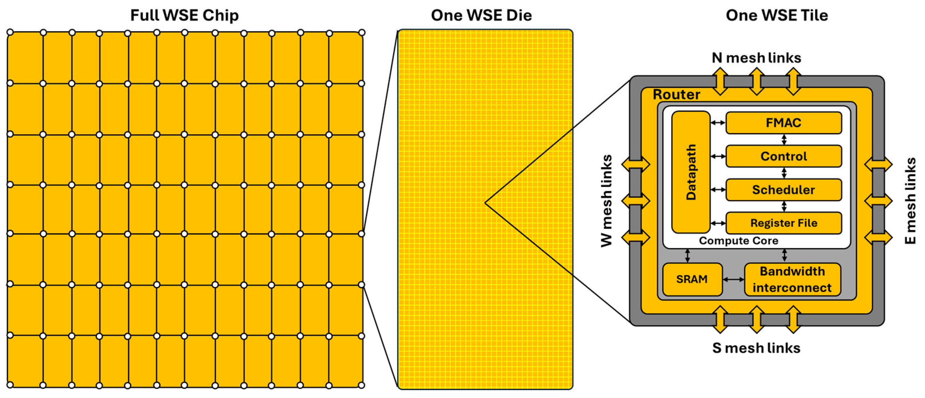
Figure 1. Hierarchical structure of the WSE, showing the full processor (left), an array of interconnected dies (middle), and the internal structure of single processing element (right).
Energies 18 05874 g001
Figure 2. Comparison between the chip size of WSE CS-2 and that of the largest graphic processing unit (GPU).
Energies 18 05874 g002
Figure 3. CO2 properties: density, viscosity, and the formation volume factor as a function of pressure.
Energies 18 05874 g003
Figure 4. Illustration of Corey-type relative permeability curves corresponding to the parameters used in Equation (7) [6]. The figure is provided for visual reference.
Energies 18 05874 g004
Figure 5. Visualization of simulation domain decomposition: a 3D simulation grid (left) is mapped onto a 2D WSE PE-processing fabric (right).
Energies 18 05874 g005
Figure 6. Model domain used in simulation (left) and initial pressure distribution is set to hydrostatic equilibrium (right).
Energies 18 05874 g006
Figure 7. CO2 plume evolution in the storage formation at different timesteps. The cell size is 120.97 m in the horizontal direction, and 9.26 m in the vertical direction.
Energies 18 05874 g007
Figure 8. Comparison of compute time between WSE simulator and GEOS on traditional HPC for the base case. The green dashed line is a fitted reference line that represents the best runtime as cores increase.
Energies 18 05874 g008
Figure 9. CO2 plume evolution in storage formation at different timesteps using refined grid. The cell size is 60.48 m in the horizontal direction, and 9.26 m in the vertical direction.
Energies 18 05874 g009
Figure 10. Comparison of processing time between WSE simulator and GEOS on traditional HPC for the refined mesh. The green dashed line is a fitted reference line that represents the best runtime as cores increase.
Energies 18 05874 g010
Table 1. Performance comparison between base case and refined mesh.
ParameterBase MeshRefined Mesh
Grid resolution124 × 124 × 108248 × 248 × 108
Total number of grid cells1.66 million6.64 million
Runtime of this study simulator on WSE2.82 s3.28 s
Runtime of GEOS on traditional HPC334 s1123 s
Speedup of this study simulator118×342×
Number of cores used on WSE15,376 (1.8% of full WSE capacity)61,504 (7.2% of full WSE capacity)
Table 2. Comparison of reservoir simulation approaches.
FeatureFull-Physics SimulatorsML SimulatorsWSE-Based Simulator
ApproachSolves PDEs using numerical methodsLearn patterns from dataSolves PDEs using finite difference on WSE hardware
AccuracyHigh (physics-based)Variable (depends on training data)High (physics-based)
SpeedSlow (hours to days)Fast (seconds to minutes)Super-fast (seconds)
Data requirementModerate (reservoir description)Very high (large datasets)Moderate (reservoir description)
GeneralizabilityHigh (physics-based)Low–medium (limited to trained domains)High (physics-based)
HardwareCPU/GPUGPU/TPUWSE (Wafer-Scale Engine)
LimitationsLong runtimesRequires training, limited physics insightsLegacy simulator needs to be adapted to run on WSE
Disclaimer/Publisher’s Note: The statements, opinions and data contained in all publications are solely those of the individual author(s) and contributor(s) and not of MDPI and/or the editor(s). MDPI and/or the editor(s) disclaim responsibility for any injury to people or property resulting from any ideas, methods, instructions or products referred to in the content.