
China’s Low-Carbon City Pilot Policy, Eco-Efficiency, and Energy Consumption: Study Based on Period-by-Period PSM-DID Model
Abstract
1. Introduction
2. Literature Review
3. Methods
3.1. Eco-Efficiency Model
3.2. Classical DID Model
3.3. Time-Varying DID Model
4. Data Sources
5. Benchmark Analysis Results
5.1. Parallel Trend Test
5.2. Time-Varying DID
6. Robustness Test
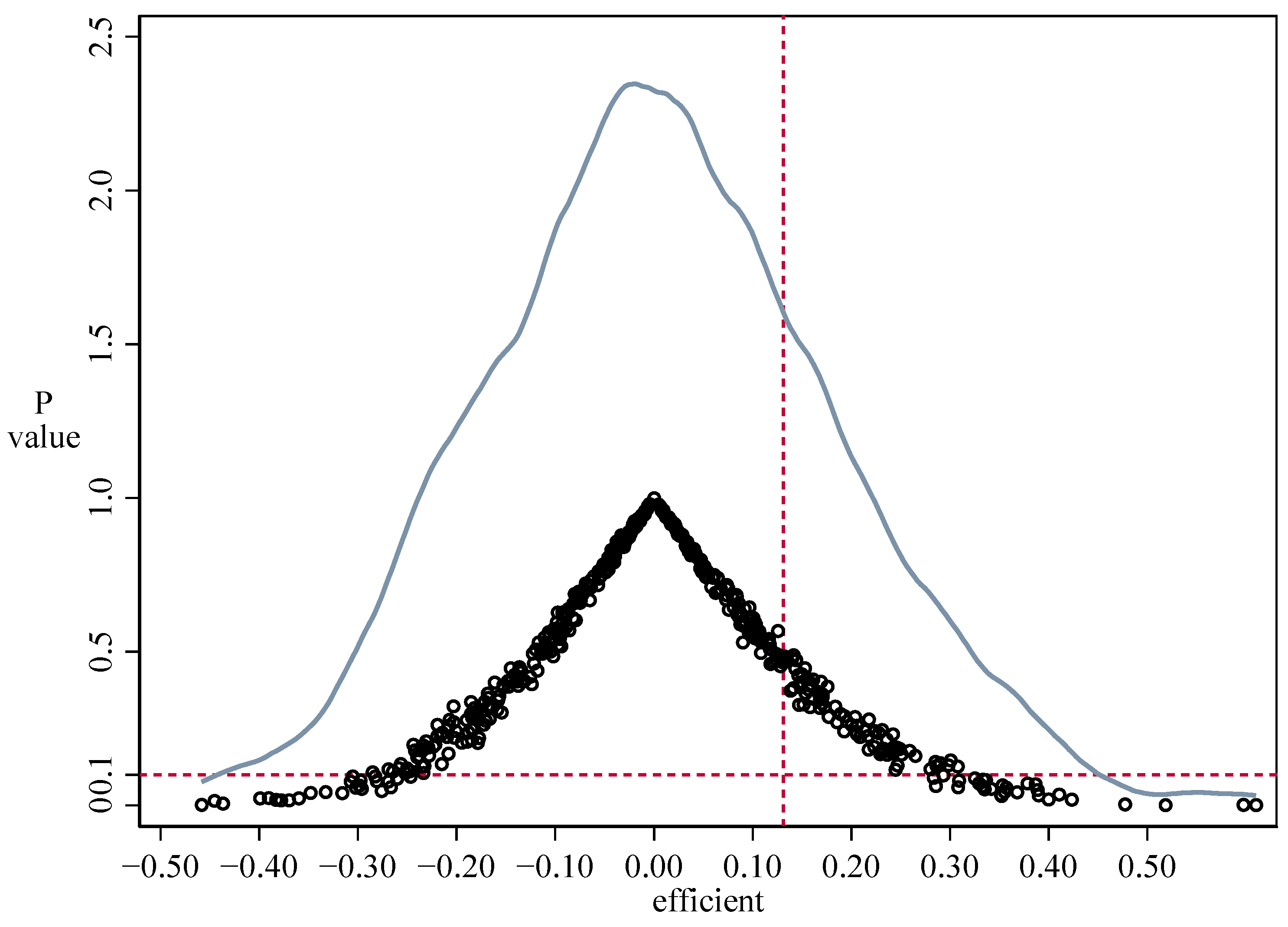
6.1. Placebo Test
6.1.1. Change the Timing of Policies
6.1.2. Fictional Intervention Group
6.1.3. Randomize Policy Time and Sample of the Intervention Group at the Same Time
6.2. Endogeneity Problem: Period-by-Period PSM-DID
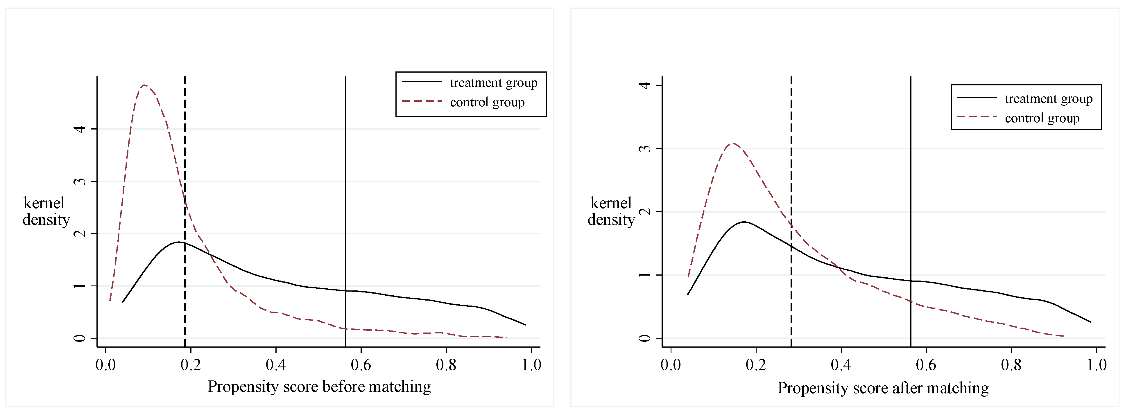
6.2.1. Preference Score Matching
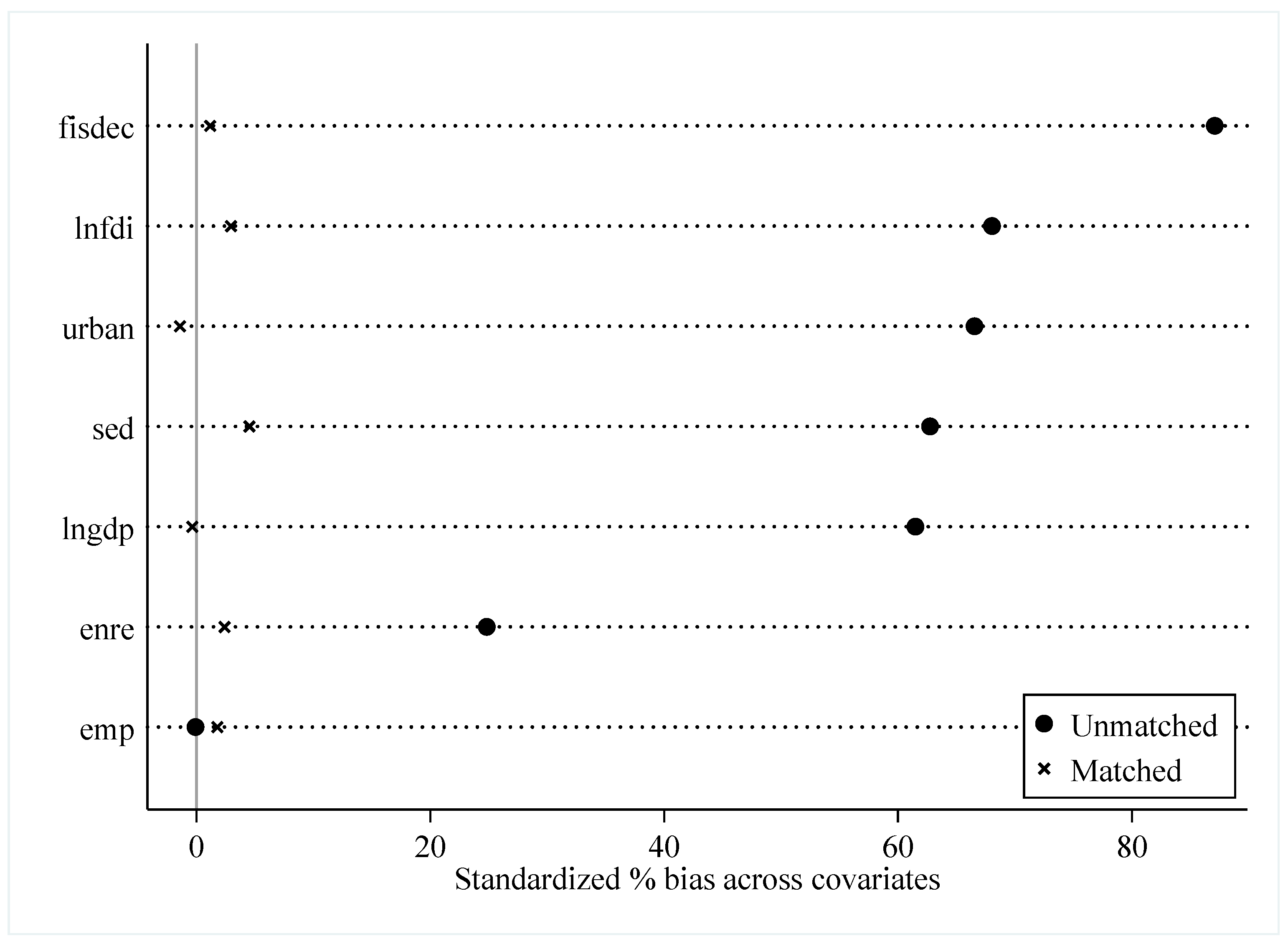
6.2.2. Balance Test
6.2.3. PSM-DID Analysis
6.2.4. Replace the Dependent Variable
6.2.5. Modify the Desired and Undesired Outputs in the Eco-Efficiency Model
7. Heterogeneity Analysis
7.1. Comparison of Effects in Different Regions
7.2. Comparison of Effects of Different Batches
7.3. Comparison of Effects in Pilot Provinces
8. Path Analysis
9. Conclusions
- (1)
- Strengthen clean energy incentive policies: The government should increase subsidies for solar, wind, hydro, and biomass energy. For example, provide financial support to companies building solar power plants to reduce their initial construction costs and boost the share of clean energy in the energy consumption mix. Implement tax incentives for clean energy production, offering reduced corporate income tax for businesses engaged in clean energy production, encouraging them to expand their clean energy operations. Establish a green power certificate trading system to incentivize companies to produce more clean energy through market mechanisms, while also meeting the demand for green energy from high-energy-consuming enterprises, promoting a greener transformation of the energy consumption structure.
- (2)
- Enhance environmental standards for traditional energy: Strictly set emission standards for the use of coal, oil, and other traditional energy sources. Require companies to install advanced pollution control equipment to reduce pollutant emissions. Impose severe penalties such as hefty fines and production halts on non-compliant enterprises, compelling them to reduce reliance on high-pollution traditional energy. Raise the environmental entry threshold for traditional energy extraction, restricting large-scale mining activities that cause significant ecological damage, such as small coal mines and oil fields, to control the impact of traditional energy on the environment at its source. Promote technological upgrades in traditional energy companies to improve energy efficiency and lower pollutant emissions per unit of energy consumption.
- (3)
- Promote the diversification of energy consumption: Encourage businesses and residents to use multiple energy sources, reducing over-reliance on a single type. Promote the supply of natural gas, electricity, and other energy options in cities, offering users more choices. Support the development of distributed energy systems, such as constructing photovoltaic and wind power facilities in industrial parks and commercial complexes, to achieve local production and consumption of energy, enhancing the flexibility and reliability of energy utilization. Strengthen research and application of energy storage technologies, like battery storage, to address the intermittency issues of clean energy generation, promoting the stable and diversified development of energy consumption.
- (4)
- Guide enterprises towards green energy transition: The government can establish special funds to provide low-interest loans or financial support for companies transitioning to green energy, helping them purchase clean energy equipment and conduct technological research and development. Enterprises that actively transition should be given policy incentives, such as priority in energy supply and convenience in project approval. Organize industry associations and research institutions to offer technical consulting and training services for enterprises, assisting them in overcoming technical challenges during the transition. Through policy guidance, encourage enterprises to prioritize the use of clean energy in production processes, gradually reducing their reliance on traditional energy sources.
- (5)
- Strengthen the supervision of environmental regulation policies: Establish a dedicated supervisory body for the enforcement of environmental regulations to enhance daily oversight of corporate energy consumption. Utilize big data and Internet of Things technology to monitor real-time energy consumption and pollutant emissions from companies, ensuring strict compliance with environmental regulations. Hold accountable any departments or individuals who fail in their supervisory duties, enhancing the seriousness and effectiveness of policy implementation. Regularly publish information on corporate energy consumption and compliance with environmental regulations to foster public scrutiny, creating an atmosphere of societal participation that promotes the optimization of energy consumption structures and improves eco-efficiency.
- (6)
- The coordination of carbon pricing mechanisms and green financial instruments: Institutional design, market mechanisms, and financial innovation can form a synergistic closed loop of “policy guidance–market pricing–financial empowerment”. With the carbon pricing mechanism as the core, resource allocation is guided through market signals; green financial instruments are used as a lever to amplify the incentive effect of policies; and institutional innovation is taken as a guarantee to solve the problems of inter-departmental and cross-regional coordination. The carbon emission statistical accounting system of pilot cities needs to be aligned with the MRV standards of the national carbon market. For example, Huzhou City has established a “1 + 4” carbon emission control system, linking regional carbon budgets with quota allocation in the national market. Pilot cities should develop diversified financial instruments based on underlying assets such as carbon allowances, carbon sinks, and carbon footprints.
Author Contributions
Funding
Data Availability Statement
Conflicts of Interest
References
- Schaltegger, S.; Sturm, A. Kologische rationalitt (German/in English: Environmental Rationality). Die Unternehm. 1990, 4, 117–131. [Google Scholar]
- Sustainable development goals. In The Energy Progress Report; Tracking SDG: New York, NY, USA, 2019; Volume 7, pp. 2–6.
- Li, Y.; Li, H.; Miao, R.; Qi, H.; Zhang, Y. Energy–Environment–Economy (3E) Analysis of the Performance of Introducing Photovoltaic and Energy Storage Systems into Residential Buildings: A Case Study in Shenzhen, China. Sustainability 2023, 15, 9007. [Google Scholar] [CrossRef]
- Li, T.; Li, Y. Artificial intelligence for reducing the carbon emissions of 5G networks in China. Nat. Sustain. 2023, 6, 1522–1523. [Google Scholar] [CrossRef]
- Yu, Z.; Ning, Z.; Zhang, H.; Yang, H.; Chang, S.J. A generalized Faustmann model with multiple carbon pools. For. Policy Econ. 2024, 169, 103363. [Google Scholar] [CrossRef]
- Yu, Z.; Ning, Z.; Chang, W.Y.; Chang, S.J.; Yang, H. Optimal harvest decisions for the management of carbon sequestration forests under price uncertainty and risk preferences. For. Policy Econ. 2023, 151, 102957. [Google Scholar] [CrossRef]
- Yang, H.; Zhang, X.; Hong, Y. Classification, production, and carbon stock of harvested wood products in China from 1961 to 2012. BioResources 2014, 9, 4311–4322. Available online: http://ncsu.edu/bioresources/BioRes_09/BioRes_09_3_4311_Yang_Zhang_Hong_Classif_Prodn_Carbon_Stock_5108.pdf (accessed on 29 May 2025). [CrossRef]
- Li, X.; Ning, Z.; Yang, H. A review of the relationship between China’s key forestry ecology projects and carbon market under carbon neutrality. Trees For. People 2022, 9, 100311. [Google Scholar] [CrossRef]
- Li, B.; Wang, X.; Khurshid, A.; Saleem, S.F. Environmental governance, green finance, and mitigation technologies: Pathways to carbon neutrality in European industrial economies. Int. J. Environ. Sci. Technol. 2025, 1–14. [Google Scholar] [CrossRef]
- Porter, M.E. Towards a dynamic theory of strategy. Strateg. Manag. J. 1991, 12, 95. [Google Scholar] [CrossRef]
- Zhao, Y.; Zhu, F.; He, L. Definition, Classification and Evolution of Environmental Regulation. China Popul. Resour. Environ. 2009, 19, 6. [Google Scholar]
- Li, X.; Pan, J. The Compilation of China’s Green Development Index—Annual Report on China’s Green Development Index 2010—Provincial Comparison. Econ. Res. Ref. 2011, 2, 29. [Google Scholar]
- Moutinho, V.; Madaleno, M. Assessing Eco-Efficiency in Asian and African Countries Using Stochastic Frontier Analysis. Energies 2021, 14, 1168. [Google Scholar] [CrossRef]
- Xu, A.; Wang, W.; Zhu, Y. Does smart city pilot policy reduce CO2 emissions from industrial firms? Insights from China. J. Innov. Knowl. 2023, 8, 100367. [Google Scholar] [CrossRef]
- Li, S.; Chu, S.; Shen, C. Local Government Competition, Environmental Regulation and Regional eco-efficiency. World Econ. 2014, 4, 23. [Google Scholar]
- Luo, N.; Wang, Y. Fiscal decentralization, environmental regulation and regional eco-efficiency—An empirical study based on dynamic spatial Durbin model. China Popul. Resour. Environ. 2017, 27, 110–118. [Google Scholar]
- Wang, R.; Sun, T. Research on the Impact of Environmental Regulation on China’s Regional Green Economic Efficiency Based on Super-Efficiency DEA Model. Ecol. Econ. 2019, 35, 6. [Google Scholar]
- Fang, Q. The Impact of Environmental Policy on Low-Carbon Technology Innovation Performance of Chinese Manufacturing Industry. In Advances in Social Science, Education and Humanities Research; Atlantis Press: Dordrecht, The Netherlands, 2015; Volume 31, pp. 44–50. [Google Scholar]
- You, D.; Ouyang, L. The Impact of Environmental Regulation on the Green Innovation Efficiency of Industrial Enterprises—An Empirical Analysis Based on Spatial Durbin Model. Reform 2020, 5, 17. [Google Scholar]
- Charnes, A.; Cooper, W.W.; Rhodes, E. A Data Envelopment Analysis Approach to Evaluation of the Program Follow through Experiment in U.S. Public School Education. 1978. Available online: https://iiif.library.cmu.edu/file/Cooper_box00016_fld00023_bdl0001_doc0002/Cooper_box00016_fld00023_bdl0001_doc0002.pdf (accessed on 30 May 2025).
- Malmquist, S. Index numbers and indifference surfaces. Trabajos de Estadistica 1953, 4, 209–242. [Google Scholar] [CrossRef]
- Färe, R.; Grosskopf, S.; Lindgren, B.; Roos, P. Productivity changes in Swedish pharamacies 1980–1989: A non-parametric Malmquist approach. J. Prod. Anal. 1992, 3, 85–101. [Google Scholar] [CrossRef]
- Berg, S.A.; Førsund, F.R.; Jansen, E.S. Malmquist Indices of Productivity Growth during the Deregulation of Norwegian Banking, 1980–1989. Scand. J. Econ. 1992, 94, S211–S228. [Google Scholar] [CrossRef]
- Xie, S.; Fan, P.; Wan, Y. Improvement and Application of Traditional PSM-DID Model. Stat. Res. 2021, 38, 15. [Google Scholar]
- Li, Q.; Xiao, Z. Heterogeneous Environmental Regulation Tools and Corporate Green Innovation Incentives—Evidence from Green Patents of Listed Companies. Econ. Res. 2020, 55, 17. [Google Scholar]
- Arkhangelsky, D.; Athey, S.; Hirshberg, D.A.; Imbens, G.W.; Wager, S. Synthetic Difference-in-Differences. Am. Econ. Rev. 2021, 111, 4088–4118. [Google Scholar] [CrossRef]
- Huang, J.; Zheng, B.; Du, M. How digital economy mitigates urban carbon emissions: The green facilitative power of industrial coagglomeration. Appl. Econ. 2025, 1–19. [Google Scholar] [CrossRef]


| Categories | Indicators | Code | Specific Indicators Constitute |
|---|---|---|---|
| Input factors | Capital | CI | Investment in fixed assets (CNY 100 million) |
| Labor force | LI | Total number of employees (10 thousand) | |
| Science and technology | SI | Expenditure on science and technology (CNY 10 thousand) | |
| The sources of energy | EI | Annual electricity consumption (10,000 KWH) | |
| Expected outputs | Economic output | EC | Per capita GDP (CNY 10 thousand) |
| Green output | GR | Park green area (square meters) | |
| Unexpected outputs | Pollution output | AQI | Air Quality Index (AQI) |
| Indicator | Variable | Definitions |
|---|---|---|
| MI | Eco-efficiency | The Malmquist productivity index with non-expected output |
| LnGdp | Level of economic development | Logarithm of GDP per capita |
| Urban | Urbanization level | Urban resident population/total resident population |
| FisDec | Degree of fiscal decentralization | General revenue of government finance/general expenditure of government finance |
| SEd | Spending on science and technology | Science and technology expenditure/general government expenditure |
| EnRe | Degree of environmental regulation | Comprehensive utilization rate of general industrial solid waste |
| Emp | Employment structure | Number of employees in the tertiary industry/total number of employees |
| Variable | Obs | Mean | Std. Dev. | Min | Max |
|---|---|---|---|---|---|
| MI | 5282 | 2.7220 | 2.0410 | 0.3130 | 10.7490 |
| LnGdp | 5282 | 10.2710 | 0.8900 | 8.2760 | 12.4340 |
| Urban | 5282 | 0.5030 | 0.1720 | 0.1580 | 0.9460 |
| FisDec | 5282 | 0.4710 | 0.2210 | 0.1090 | 1.0240 |
| SEd | 5282 | 0.0130 | 0.0140 | 0.0010 | 0.0750 |
| EnRe | 5282 | 79.9130 | 22.4620 | 10.3600 | 114.8500 |
| Emp | 5282 | 0.5480 | 0.1340 | 0.2250 | 0.8640 |
| Classical DID | Time-Varying DID | |||||
|---|---|---|---|---|---|---|
| Dit | 2.349 *** (0.095) | 0.374 *** (0.067) | 2.435 *** (0.097) | 0.385 *** (0.067) | 0.321 *** (0.072) | 0.131 ** (0.065) |
| LnGdp | 1.828 *** (0.039) | 1.820 *** (0.039) | 2.232 *** (0.065) | |||
| Urban | 1.339 *** (0.219) | 1.882 *** (0.225) | 0.989 *** (0.220) | |||
| FisDec | −1.234 *** (0.170) | −0.510 *** (0.193) | −0.219 (0.192) | |||
| SEd | −13.978 *** (1.807) | −13.613 *** (1.808) | −6.419 *** (1.781) | |||
| EnRe | 0.001 (0.001) | 0.002 * (0.001) | 0.005 *** (0.001) | |||
| Emp | 3.595 *** (0.192) | 3.636 *** (0.197) | 2.452 *** (0.201) | |||
| Individual-fixed | No | No | Yes | Yes | Yes | Yes |
| Time-fixed | No | No | No | No | Yes | Yes |
| R-squared | 0.059 | 0.347 | 0.112 | 0.647 | 0.583 | 0.682 |
| Observations | 5282 | 5282 | 5282 | 5282 | 5282 | 5282 |
| Pre3 | Pre2 | Pre1 | Lat1 | Lat2 | |
|---|---|---|---|---|---|
| Dit | 0.073 (0.062) | 0.068 (0.062) | 0.057 (0.064) | 0.144 ** (0.067) | 0.144 ** (0.071) |
| Individual-fixed | Yes | Yes | Yes | Yes | Yes |
| Time-fixed | Yes | Yes | Yes | Yes | Yes |
| R-squared | 0.682 | 0.682 | 0.682 | 0.682 | 0.682 |
| Observations | 5282 | 5282 | 5282 | 5282 | 5282 |
| Unmatched | Mean | %Reduct | t-Test | V(T)/V(C) | ||||
|---|---|---|---|---|---|---|---|---|
| Variable | Matched | Treated | Control | %bias | bias | t | p > t | |
| Lngdp | U | 10.683 | 10.141 | 61.5 | 19.59 | 0 | 1.21 * | |
| M | 10.582 | 10.586 | −0.4 | 99.4 | −0.09 | 0.93 | 0.89 * | |
| Urban | U | 0.59055 | 0.47505 | 66.5 | 21.74 | 0 | 1.45 * | |
| M | 0.56682 | 0.56929 | −1.4 | 97.9 | −0.33 | 0.745 | 0.93 | |
| Fisdec | U | 0.61282 | 0.42596 | 87.1 | 28.2 | 0 | 1.36 * | |
| M | 0.58791 | 0.58541 | 1.2 | 98.7 | 0.27 | 0.79 | 1 | |
| Sed | U | 0.02036 | 0.01084 | 62.7 | 22.28 | 0 | 2.64 * | |
| M | 0.01802 | 0.01733 | 4.5 | 92.8 | 1 | 0.318 | 0.89 | |
| Enre | U | 83.873 | 78.656 | 24.8 | 7.25 | 0 | 0.60 * | |
| M | 83.504 | 83.001 | 2.4 | 90.4 | 0.62 | 0.535 | 0.84 * | |
| Emp | U | 0.54781 | 0.54793 | −0.1 | −0.03 | 0.979 | 1.03 | |
| M | 0.53999 | 0.53761 | 1.8 | −2006.4 | 0.42 | 0.675 | 0.92 | |
| Lnfdi | U | 10.693 | 9.3412 | 68 | 21.6 | 0 | 1.17 * | |
| M | 10.492 | 10.433 | 3 | 95.7 | 0.78 | 0.438 | 1.54 * | |
| (1) | (2) | (3) | (4) | (5) | (6) | (7) | (8) | (9) | (10) | |
|---|---|---|---|---|---|---|---|---|---|---|
| 2003b | 2004b | 2005b | 2006b | 2007b | 2008b | 2009b | 2010b | 2011b | 2012b | |
| LnGdp | 0.4342 | 0.2764 | 0.2703 | −0.3248 | −0.4567 | −0.2328 | −0.1824 | −0.0672 | −0.1060 | −0.3630 |
| (0.9743) | (0.6023) | (0.6343) | (−0.7216) | (−0.8859) | (−0.4675) | (−0.3588) | (−0.1369) | (−0.2111) | (−0.7252) | |
| Urban | 0.3887 | 0.7319 | 2.0257 * | 1.9125 | 1.8362 | 1.6898 | 2.9644 ** | 4.4656 *** | 3.5278 ** | 4.1952 *** |
| (0.3490) | (0.6782) | (1.7335) | (1.3972) | (1.3009) | (1.0823) | (1.9966) | (2.9930) | (2.5077) | (2.6047) | |
| FisDec | 4.1379 *** | 4.1090 *** | 3.5619 ** | 5.1433 *** | 2.6408 ** | 0.8521 | 0.9585 | 0.1302 | 2.0043 | 2.9139 * |
| (3.1505) | (3.0738) | (2.4723) | (3.3534) | (2.0128) | (0.7731) | (0.6128) | (0.0866) | (1.3152) | (1.8540) | |
| SEd | −63.9245 | −76.4230 | −98.4929 | −16.4236 | 56.1680 ** | 74.2951 *** | 66.0572 * | 49.3896 * | 32.1914 * | 18.8283 |
| (−0.9483) | (−1.3628) | (−1.4370) | (−0.1729) | (2.1501) | (2.9410) | (1.8103) | (1.8786) | (1.8151) | (1.1183) | |
| EnRe | 0.0020 | 0.0026 | 0.0048 | 0.0009 | 0.0005 | −0.0005 | 0.0033 | 0.0045 | 0.0064 | 0.0017 |
| (0.2909) | (0.3831) | (0.6749) | (0.1190) | (0.0664) | (−0.0738) | (0.4193) | (0.5805) | (0.7936) | (0.2350) | |
| Emp | 3.6022 ** | 3.0268 ** | 4.3901 *** | 4.2069 *** | 3.5034 ** | 3.6692 ** | 3.6561 ** | 4.1012 *** | 4.2836 *** | 3.7583 ** |
| (2.3996) | (2.1174) | (3.0546) | (2.8544) | (2.2632) | (2.2574) | (2.3911) | (2.7869) | (2.7115) | (2.5206) | |
| Lnfdi | 0.0731 | 0.1136 | 0.0900 | 0.0761 | 0.1131 | 0.1824 | 0.0405 | 0.0735 | 0.0619 | 0.0494 |
| (0.5605) | (0.9032) | (0.7408) | (0.5441) | (0.7711) | (1.2304) | (0.2527) | (0.4398) | (0.3966) | (0.3335) | |
| N | 278 | 278 | 278 | 278 | 278 | 278 | 278 | 278 | 278 | 278 |
| Pseudo R2 | 0.1619 | 0.1622 | 0.1746 | 0.1775 | 0.1748 | 0.1760 | 0.1807 | 0.1788 | 0.1793 | 0.1709 |
| (11) | (12) | (13) | (14) | (15) | (16) | (17) | (18) | (19) | ||
| 2013b | 2014b | 2015b | 2016b | 2017b | 2018b | 2019b | 2020b | 2021b | ||
| LnGdp | −0.1403 | −0.1236 | −0.6166 | −0.3863 | −0.2820 | 0.3894 | 0.6336 | 0.3605 | 1.0948 * | |
| (−0.2694) | (−0.2302) | (−1.0597) | (−0.6638) | (−0.4611) | (0.6356) | (0.9176) | (0.5818) | (1.9218) | ||
| Urban | 4.2759 ** | 4.2518 ** | 5.4612 *** | 5.6291 *** | 5.8614 *** | 6.0809 *** | 5.4680 ** | 4.8506 *** | 3.0866 ** | |
| (2.2750) | (2.3290) | (2.5932) | (2.6563) | (2.6860) | (2.6382) | (2.4023) | (2.5887) | (1.9743) | ||
| FisDec | 1.4783 | 2.0088 | 4.2192 *** | 3.5938 ** | 2.2585 | 0.1652 | −0.2841 | 1.2378 | −0.7433 | |
| (0.8823) | (1.1957) | (2.5817) | (2.0653) | (1.3032) | (0.0915) | (−0.1452) | (0.6527) | (−0.4297) | ||
| SEd | 36.1144 * | 23.0323 * | 18.8759 | 13.2753 | 15.7110 | 16.9796 | 18.0523 | 22.9261 * | 16.9138 | |
| (1.7787) | (1.6644) | (1.2368) | (1.0405) | (1.1249) | (1.2282) | (1.3441) | (1.7251) | (1.4978) | ||
| EnRe | 0.0057 | 0.0079 | 0.0027 | 0.0038 | 0.0097 | 0.0134 | 0.0078 | 0.0110 | 0.0095 | |
| (0.6586) | (0.9138) | (0.3505) | (0.4890) | (1.1520) | (1.5923) | (0.9412) | (1.2525) | (1.1552) | ||
| Emp | 6.0189 *** | 5.8113 *** | 5.9136 *** | 5.9587 *** | 5.4924 *** | 5.2800 *** | 6.0372 *** | 5.9990 *** | 4.4083 *** | |
| (3.4929) | (3.6523) | (3.5347) | (3.6565) | (3.8272) | (3.7749) | (3.9170) | (4.0298) | (3.1742) | ||
| Lnfdi | 0.1566 | 0.1777 | 0.0339 | 0.0880 | 0.2009 * | 0.1297 | 0.1906 * | 0.0843 | 0.1414 | |
| (1.0699) | (1.3153) | (0.2424) | (0.6853) | (1.6600) | (1.3004) | (1.9150) | (0.6595) | (1.1070) | ||
| Observations | 278 | 278 | 278 | 278 | 278 | 278 | 278 | 278 | 278 | |
| Pseudo R2 | 0.2039 | 0.2063 | 0.2313 | 0.2301 | 0.2364 | 0.2309 | 0.2399 | 0.2436 | 0.2160 |
| (1) | (2) | (3) | (4) | (5) | (6) | (7) | (8) | (9) | (10) | |
|---|---|---|---|---|---|---|---|---|---|---|
| 2003a | 2004a | 2005a | 2006a | 2007a | 2008a | 2009a | 2010a | 2011a | 2012a | |
| LnGdp | −0.5644 | 0.3158 | 0.1415 | −0.3440 | −0.2104 | −0.3924 | 0.2443 | 0.4435 | −0.0491 | 0.4313 |
| (−1.0706) | (0.5727) | (0.2525) | (−0.5563) | (−0.3460) | (−0.6547) | (0.3711) | (0.7471) | (−0.0833) | (0.6917) | |
| Urban | 2.9719 * | 0.4499 | 0.4826 | 1.2663 | 0.0695 | 0.5744 | −1.3892 | −0.5900 | 0.5963 | 0.0711 |
| (1.8151) | (0.3025) | (0.3114) | (0.7559) | (0.0437) | (0.3523) | (−0.7733) | (−0.2853) | (0.3528) | (0.0375) | |
| FisDec | 1.8020 | 0.8046 | 1.0440 | 1.7973 | 0.0306 | 1.4796 | −0.8514 | −0.7574 | 0.6342 | −0.9004 |
| (1.0965) | (0.5155) | (0.6671) | (1.0351) | (0.0213) | (0.9520) | (−0.4492) | (−0.4681) | (0.3519) | (−0.4504) | |
| SEd | −1.1 × 10² | 67.3873 | −1.6 × 10² | −62.6711 | 36.4138 | 24.3065 | 63.2775 * | 16.3786 | 16.4340 | 14.1040 |
| (−1.0326) | (0.5536) | (−1.3843) | (−0.5698) | (1.0480) | (0.7342) | (1.9279) | (0.5081) | (0.8631) | (0.6690) | |
| EnRe | −0.0057 | 0.0022 | 0.0004 | −0.0013 | −0.0059 | −0.0100 | 0.0028 | −0.0012 | −0.0005 | −0.0042 |
| (−0.5630) | (0.2377) | (0.0423) | (−0.1381) | (−0.6445) | (−0.9608) | (0.2893) | (−0.1302) | (−0.0440) | (−0.3969) | |
| Emp | 0.5059 | 1.0754 | 0.5182 | 0.4560 | −0.0601 | 0.3310 | −0.0781 | 0.2364 | 2.0201 | −0.3492 |
| (0.2700) | (0.5293) | (0.2675) | (0.2482) | (−0.0327) | (0.1606) | (−0.0417) | (0.1261) | (1.2213) | (−0.1803) | |
| Lnfdi | 0.1127 | −0.0109 | −0.0365 | −0.0164 | 0.0523 | 0.0239 | −0.1226 | 0.0708 | 0.0138 | 0.0842 |
| (0.7967) | (−0.0813) | (−0.2809) | (−0.1221) | (0.3550) | (0.1581) | (−0.7439) | (0.4544) | (0.0797) | (0.5122) | |
| N | 126 | 124 | 128 | 132 | 126 | 125 | 121 | 122 | 125 | 122 |
| Pseudo R2 | 0.0422 | 0.0223 | 0.0167 | 0.0139 | 0.0151 | 0.0272 | 0.0384 | 0.0165 | 0.0192 | 0.0288 |
| (11) | (12) | (13) | (14) | (15) | (16) | (17) | (18) | (19) | ||
| 2013a | 2014a | 2015a | 2016a | 2017a | 2018a | 2019a | 2020a | 2021a | ||
| LnGdp | 0.4430 | 0.1624 | −0.0744 | 0.3967 | −0.1503 | −0.0198 | −0.4536 | 0.3098 | −0.2524 | |
| (0.6754) | (0.2284) | (−0.0995) | (0.5365) | (−0.1866) | (−0.0255) | (−0.5577) | (0.4259) | (−0.3508) | ||
| Urban | 1.7801 | −0.1778 | −0.3741 | −1.7313 | 2.7618 | 1.4108 | 2.9449 | 1.4836 | 0.7025 | |
| (0.8201) | (−0.0739) | (−0.1308) | (−0.5935) | (0.8707) | (0.4786) | (1.0111) | (0.5682) | (0.3041) | ||
| FisDec | −1.0076 | 0.7001 | 1.5238 | 0.6489 | −0.2337 | −1.5095 | 1.9261 | −0.7422 | 1.6424 | |
| (−0.5086) | (0.3590) | (0.8354) | (0.3392) | (−0.1126) | (−0.8488) | (0.9870) | (−0.3263) | (0.8473) | ||
| SEd | −8.1101 | 15.7087 | 10.4282 | −7.8896 | 15.1155 | 22.2366 | 4.5677 | 5.3367 | 15.6782 | |
| (−0.3741) | (0.8765) | (0.6328) | (−0.5140) | (0.9115) | (1.3188) | (0.3267) | (0.3603) | (1.0938) | ||
| EnRe | −0.0032 | −0.0046 | 0.0008 | −0.0042 | 0.0012 | 0.0018 | 0.0046 | 0.0068 | −0.0015 | |
| (−0.3004) | (−0.4406) | (0.0865) | (−0.4239) | (0.1234) | (0.1932) | (0.4668) | (0.6951) | (−0.1510) | ||
| Emp | 1.2598 | 1.5582 | 1.4378 | 0.1775 | 0.2813 | 1.7815 | 1.9490 | 2.1347 | 0.6847 | |
| (0.6801) | (0.8756) | (0.7763) | (0.0812) | (0.1535) | (1.0215) | (1.0504) | (1.0993) | (0.4103) | ||
| Lnfdi | 0.0821 | −0.0964 | −0.0634 | 0.1201 | −0.1561 | 0.0817 | −0.0554 | 0.0374 | −0.0856 | |
| (0.4994) | (−0.5277) | (−0.4022) | (0.8250) | (−0.9853) | (0.5894) | (−0.4026) | (0.2132) | (−0.4956) | ||
| Observations | 124 | 120 | 115 | 114 | 114 | 119 | 129 | 115 | 120 | |
| Pseudo R2 | 0.0205 | 0.0152 | 0.0124 | 0.0201 | 0.0246 | 0.0280 | 0.0291 | 0.0215 | 0.0266 |
| (1) | (2) | (3) | (4) | (5) | |
|---|---|---|---|---|---|
| Classical DID | Time-Varying DID | PSM-DID (1) | PSM-DID (2) | PSM-DID (3) | |
| Dit | 0.4456 *** | 0.1307 ** | 0.2694 *** | 0.1849 *** | 0.3165 *** |
| (5.1248) | (2.0145) | (3.3393) | (2.7208) | (4.3162) | |
| Individual-fixed | No | Yes | Yes | Yes | Yes |
| Time-fixed | No | Yes | Yes | Yes | Yes |
| Observations | 5282 | 5282 | 2321 | 4531 | 3313 |
| Adj. R2 | 0.3880 | 0.7871 | 0.7976 | 0.7946 | 0.8231 |
| (1) | (2) | (3) | (4) | (5) | |
|---|---|---|---|---|---|
| Classical DID | Time-Varying DID | PSM-DID (1) | PSM-DID (2) | PSM-DID (3) | |
| Dit | 0.4016 *** | 0.2702 *** | 0.1335 *** | 0.1826 *** | 0.0818 *** |
| (9.7883) | (10.1511) | (4.2065) | (7.3619) | (2.7464) | |
| Observations | 5282 | 5282 | 2321 | 4531 | 3313 |
| Adj. R2 | 0.2044 | 0.7909 | 0.7805 | 0.7844 | 0.7974 |
| PM2.5 as Undesirable Output | |||||
|---|---|---|---|---|---|
| (1) | (2) | (3) | (4) | (5) | |
| OLS | FE | Weight not vacancy. | On_Support | Weight_Reg | |
| dit | 0.3218 ** | 0.2974 *** | 0.2678 * | 0.3941 *** | 0.3746 *** |
| (2.4516) | (2.6238) | (1.6466) | (3.2737) | (2.7628) | |
| lngdp | 2.2797 *** | 2.7285 *** | 2.8478 *** | 2.6937 *** | 2.4925 *** |
| (32.8319) | (24.0432) | (13.6406) | (21.7015) | (15.7856) | |
| urban | −0.3482 | 0.4285 | −0.7784 | −0.0498 | −0.8630 |
| (−1.0907) | (1.1154) | (−1.1057) | (−0.1193) | (−1.6177) | |
| fisdec | −2.7827 *** | −0.3580 | −0.7857 | −0.4056 | −0.4666 |
| (−13.8887) | (−1.0685) | (−1.3868) | (−1.1402) | (−1.1346) | |
| sed | −37.0798 *** | −19.5161 *** | −24.3922 *** | −18.6950 *** | −16.9408 *** |
| (−11.0205) | (−6.2707) | (−4.6189) | (−5.4160) | (−4.4417) | |
| enre | −0.0016 | 0.0030 | 0.0028 | 0.0031 | −0.0001 |
| (−1.0615) | (1.5730) | (0.6957) | (1.4006) | (−0.0459) | |
| emp | 3.8976 *** | 3.2481 *** | 2.8911 *** | 3.7166 *** | 3.5825 *** |
| (13.8950) | (9.2556) | (4.4076) | (9.2357) | (7.5822) | |
| N | 5282 | 5282 | 2321 | 4531 | 3313 |
| Adj. R2 | 0.3007 | 0.6742 | 0.6686 | 0.6820 | 0.7201 |
| CO2 as Undesirable Output | |||||
|---|---|---|---|---|---|
| (1) | (2) | (3) | (4) | (5) | |
| OLS | FE | Weight not vacancy. | On_Support | Weight_Reg | |
| dit | 0.5556 *** | 0.4644 *** | 0.4078 ** | 0.5321 *** | 0.3746 *** |
| (4.1510) | (4.1462) | (2.4970) | (4.4282) | (2.7628) | |
| lngdp | 2.1187 *** | 2.5928 *** | 2.7297 *** | 2.6164 *** | 2.4925 *** |
| (29.9259) | (23.1229) | (13.0198) | (21.1201) | (15.7856) | |
| urban | −0.4197 | 0.5267 | −0.4477 | 0.2383 | −0.8630 |
| (−1.2892) | (1.3875) | (−0.6332) | (0.5721) | (−1.6177) | |
| fisdec | −2.4978 *** | 0.5225 | 0.1159 | 0.4635 | −0.4666 |
| (−12.2265) | (1.5779) | (0.2038) | (1.3055) | (−1.1346) | |
| sed | −38.3605 *** | −17.7336 *** | −24.2723 *** | −18.1235 *** | −16.9408 *** |
| (−11.1815) | (−5.7666) | (−4.5768) | (−5.2606) | (−4.4417) | |
| enre | 0.0040 *** | 0.0005 | −0.0039 | −0.0016 | −0.0001 |
| (2.5803) | (0.2892) | (−0.9785) | (−0.7062) | (−0.0459) | |
| emp | 2.8361 *** | 1.8024 *** | 2.5919 *** | 2.4334 *** | 3.5825 *** |
| (9.9159) | (5.1980) | (3.9348) | (6.0588) | (7.5822) | |
| N | 5282 | 5282 | 2321 | 4531 | 3313 |
| Adj. R2 | 0.2536 | 0.6734 | 0.6700 | 0.6769 | 0.7201 |
| Eastern Region | Central Region | Western Region | Northeast Region | |||||
|---|---|---|---|---|---|---|---|---|
| Time-Varying DID | PSM-DID | Time-Varying DID | PSM-DID | Time-Varying DID | PSM-DID | Time-Varying DID | PSM-DID | |
| Dit | −0.2905 *** | 0.4708 *** | 0.2344 ** | 0.3782 *** | 0.5655 *** | 0.3927 ** | 0.3696 * | 0.7957 ** |
| (−2.9692) | (3.8665) | (2.1413) | (3.0587) | (3.7921) | (2.2147) | (1.9343) | (2.1383) | |
| Individual-fixed | Yes | Yes | Yes | Yes | Yes | Yes | Yes | Yes |
| Time-fixed | Yes | Yes | Yes | Yes | Yes | Yes | Yes | Yes |
| Observations | 1634 | 1092 | 1520 | 725 | 1482 | 926 | 646 | 118 |
| Adj. R2 | 0.7847 | 0.7849 | 0.8186 | 0.8495 | 0.7956 | 0.8166 | 0.8112 | 0.8065 |
| MI | ATT | Std. Err. | t | p > t | [95% Conf. Interval] | |
|---|---|---|---|---|---|---|
| Dit | −0.21479 | 0.4102 | −0.52 | 0.601 | −1.01876 | 0.58919 |
| The First Batch | The Second Batch | The Third Batch | ||||
|---|---|---|---|---|---|---|
| Time-Varying DID | PSM-DID | Time-Varying DID | PSM-DID | Time-Varying DID | PSM-DID | |
| Dit | −0.2575 | 0.4606 ** | 0.0202 | 0.0400 | 0.1925 * | 0.2662 ** |
| (−1.5630) | (2.1649) | (0.1954) | (0.3573) | (1.8092) | (2.4254) | |
| Individual-fixed | Yes | Yes | Yes | Yes | Yes | Yes |
| Time-fixed | Yes | Yes | Yes | Yes | Yes | Yes |
| Observations | 4180 | 956 | 4465 | 3492 | 4655 | 3814 |
| Adj. R2 | 0.7675 | 0.8174 | 0.7675 | 0.7763 | 0.7708 | 0.7824 |
| Secondary Pilot Cities | Single Pilot Cities | |||
|---|---|---|---|---|
| Time-Varying DID | PSM-DID | Time-Varying DID | PSM-DID | |
| Dit | 0.1968 | 0.1660 | 0.1095 | 0.2577 *** |
| (1.3163) | (0.8980) | (1.5114) | (3.2784) | |
| Individual-fixed | Yes | Yes | Yes | Yes |
| Time-fixed | Yes | Yes | Yes | Yes |
| Observations | 1216 | 594 | 4066 | 3440 |
| Adj. R2 | 0.7858 | 0.8277 | 0.7884 | 0.7993 |
| EnerStr | MI | MI | |
|---|---|---|---|
| Dit | 0.008 ** (3.071) | 0.447 ** (4.891) | 0.428 ** (4.690) |
| EnerStr | 2.285 ** (4.595) | ||
| Sample size | 4641 | 4641 | 4641 |
| R2 | 0.152 | 0.364 | 0.367 |
| Adjusted R2 | 0.151 | 0.363 | 0.366 |
| F-value | F (7,4633) = 118.565, p = 0.000 | F (7,4633) = 378.479, p = 0.000 | F (8,4632) = 335.246, p = 0.000 |
| Process | Effect | SE | t | p | LLCI | ULCI | |
|---|---|---|---|---|---|---|---|
| Direct effect | dit⇒MI | 0.428 | 0.091 | 4.69 | 0 | 0.249 | 0.607 |
| Indirect effect | dit⇒EnerStr | 0.008 | 0.003 | 3.071 | 0.002 | 0.003 | 0.014 |
| EnerStr⇒MI | 2.285 | 0.497 | 4.595 | 0 | 1.31 | 3.26 | |
| Total effect | dit⇒MI | 0.447 | 0.091 | 4.891 | 0 | 0.268 | 0.626 |
Disclaimer/Publisher’s Note: The statements, opinions and data contained in all publications are solely those of the individual author(s) and contributor(s) and not of MDPI and/or the editor(s). MDPI and/or the editor(s) disclaim responsibility for any injury to people or property resulting from any ideas, methods, instructions or products referred to in the content. |
© 2025 by the authors. Licensee MDPI, Basel, Switzerland. This article is an open access article distributed under the terms and conditions of the Creative Commons Attribution (CC BY) license (https://creativecommons.org/licenses/by/4.0/).
Share and Cite
Li, X.N.; Chen, H.H. China’s Low-Carbon City Pilot Policy, Eco-Efficiency, and Energy Consumption: Study Based on Period-by-Period PSM-DID Model. Energies 2025, 18, 4126. https://doi.org/10.3390/en18154126
Li XN, Chen HH. China’s Low-Carbon City Pilot Policy, Eco-Efficiency, and Energy Consumption: Study Based on Period-by-Period PSM-DID Model. Energies. 2025; 18(15):4126. https://doi.org/10.3390/en18154126
Chicago/Turabian StyleLi, Xiao Na, and Hsing Hung Chen. 2025. "China’s Low-Carbon City Pilot Policy, Eco-Efficiency, and Energy Consumption: Study Based on Period-by-Period PSM-DID Model" Energies 18, no. 15: 4126. https://doi.org/10.3390/en18154126
APA StyleLi, X. N., & Chen, H. H. (2025). China’s Low-Carbon City Pilot Policy, Eco-Efficiency, and Energy Consumption: Study Based on Period-by-Period PSM-DID Model. Energies, 18(15), 4126. https://doi.org/10.3390/en18154126