Recovery Strategies for Combined Optical Storage Systems Based on System Short-Circuit Ratio (SCR) Thresholds

Abstract

The penetration rate of variable energy sources in the current power grid is increasing, with the aim being to expand the use of these energy sources and to replace the traditional black start power supply. This study investigates the black start of a photovoltaic storage joint system based on the system’s short-circuit ratio threshold. Firstly, the principles and control modes of the photovoltaic (PV) system, energy storage system (ESS), and high-voltage direct current (DC) transmission system are studied separately to build an overall model; secondly, computational determinations of the short-circuit ratio under different scenarios are introduced to analyze the strength of the system, and the virtual inertia and virtual damping of the PV system are configured based on this; finally, the change trend of the storage system’s state of charge (SOC) is computed and observed, and the limits of what the system can support in each stage are determined. An electromagnetic transient simulation model of a black start system is constructed in PSCAD/EMTDC, and according to the proposed recovery strategy, the system frequency is maintained in the range of 49.4~50.6 Hz during the entire black start process; the fluctuation in maximum frequency after the recovery of the DC transmission system is no more than 0.1%; and the fluctuation in photovoltaic power at each stage is less than 3%. In addition, all the key indexes meet the requirements for black start technology, which verifies the validity of the strategy and provides theoretical support and a practical reference for the black start of a grid with variable energy sources.

1. Introduction

With the proposal of the “double carbon” strategic goal, as well as the global energy crisis and issue of environmental pollution, power generation based on variable energy sources has become an inevitable development in future power grid development; however, the increasing proportion of variable energy sources in the power grid has brought significant challenges to the safe operation of the power grid [1]. Power generation based on variable energy sources is characterized by a high proportion of electronic power equipment, which lacks mechanical inertia and cannot respond to the perturbation of the grid under conventional control methods as well as the conventional alternating current (AC) grid; meanwhile, the increase in the penetration of variable energy sources decreases the short-circuit capacity of the system and weakens the grid’s resistance to faults, which is not conducive to safe and reliable operation of the power grid [2]. Given that the current power grid is affected by extreme weather and other factors, the probability of grid system failure increases, with local system failures occasionally leading to large-scale power outages. For example, in 2019, due to the high proportion of wind power reducing the inertia of the system, a lightning strike led to the shutdown of a 500 MW generator in London, UK, which caused a power drop to outside the system’s frequency and triggered a major blackout; in 2021, Texas, USA, experienced a major blackout due to an extreme cold wave [3]; in 2023, Brazil experienced a much larger power outage due to fault propagation in wind and solar power generation because of issues with voltage control, combined with incorrectly set protection tuning parameters [4]; and in 2025, a sudden drop in solar photovoltaic (PV) generation in Spain led to voltage destabilization, which caused widespread blackouts [5]. Therefore, the study of fast black starts after large-scale power outages in power systems is particularly important. Pumped storage plants can effectively balance the fluctuations of variable renewable energy sources by virtue of their long-term energy storage capacity, while their high power ratings also support the short-term power supply needs of the grid [6]. However, with fast start-up and flexible control, PV systems—when equipped with an energy storage system (ESS)—can replace traditional water or fuel units and perform black start tasks, significantly improving the black start capability of regional power systems, accelerating the process of grid fault recovery, improving the utilization rate of variable energy sources, and promoting the green and low-carbon development of power systems.

For variable energy sources to be involved in black starts, domestic and international scholars have mainly focused on variable energy sources’ black start capabilities, control modes, and starting strategies. Reference [7] explores the impact of light intensity uncertainty and ambient temperature on the feasibility of using PV systems as black start power sources. It provides a comprehensive framework for the involvement of PV storage systems in black start operations. Reference [8] evaluates the feasibility of using distributed power supplies for black starts in auxiliary grids and summarizes the recovery process for such operations. However, both studies focus primarily on the feasibility of PV storage systems in black start scenarios, without delving into the ESS configuration, control strategies, or other related issues.

To address the control challenges regarding PV grid connection, reference [9] implements a maximum power point tracking (MPPT) control strategy for the front-stage direct current–direct current (DC-DC) converter to achieve the maximal energy output, while the back-stage DC-AC converter utilizes constant-power and constant-energy (PQ) control to regulate the reference active and reactive power, providing a foundation for PV grid-connected control strategies. Reference [10] proposes a coordinated control strategy that combines MPPT and load tracking for wind and solar power generation. In this strategy, the variable-energy-source power station serves as a black start power source, enabling the start-up of adjacent thermal power units and enhancing the black start capability of the grid. Reference [11] presents a two-stage black start model that integrates wind turbines, PV systems, and energy storage. In the first stage, Dijkstra’s algorithm is used to determine a restoration path that meets the start-up time constraints of the generator, while in the second stage, the ESS assists in load restoration. Reference [12] proposes a grid recovery strategy for PV storage systems by integrating virtual synchronous generator (VSG) control into the PV inverter and adding damping controllers in the ESS. This approach minimizes the impact of external light and temperature variations while enhancing system inertia. Reference [13] proposes a novel energy management system that is capable of prioritizing the use of solar energy, as well as integrating energy storage and fuel cell technologies to enhance its black start capability and optimize the load shedding, system inertia, and renewable energy integration into distribution and transmission networks. Reference [14] proposes a black start recovery strategy for PV energy storage microgrids, which achieves inter-area state of charge (SOC) equalization through adaptive nonlinear SOC control, while optimizing the PV output and managing load fluctuations by using MPPT control to minimize battery cycling, ensure a successful black start, and prolong the battery life. Although the black start control strategies presented in these studies have been progressively refined, they primarily focus on local and regional restoration and lack a cross-regional transmission channel for post-restoration power supply.

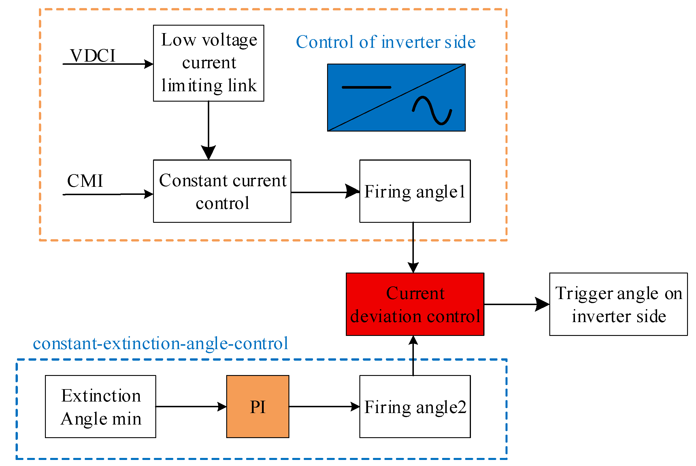
Given the problem of DC participation in the black starts of AC grids, reference [15] presents a study on the control of DC participation in black starts involving both AC and DC systems and clarifies that it is appropriate to adopt the control mode of the constant current on the rectifier side and the continuous voltage on the inverter side for DC participation in black starts. In [16], grid-type control with variable energy sources on the storage side is used to realize large-scale PV transmission via a line-commutated converter (LCC).

Based on the above research and analyses, further investigation into the black start capability of PV storage systems is necessary to ensure successful recovery under extreme conditions.

In this study, a recovery strategy for PV storage systems based on different short-circuit ratio (SCR) threshold values is proposed. The main contributions of this study are as follows:

(1)

We divide the black start stages based on the SCR calculation for the system and determine the virtual inertia and virtual damping of the PV system at each stage to enhance its inertia support to the grid.

(2)

We analyze the SOC variation in the ESS and calculate the maximum time that it can maintain safe operation during the black start process, thereby improving the success rate of the black start.

(3)

After the successful black start of the AC system, our proposed strategy continues to start the high-voltage direct-current (HVDC) transmission system to accelerate the grid reconstruction.

Section 2 of this paper outlines the development of the research model. Section 3 details the calculation method for the system’s SCR, the constraints on the SOC of the ESS, and the configuration of the virtual parameters of the PV system. Section 4 presents the simulation of the model using PSCAD/EMTDC 5.0.0 software. Finally, Section 5 provides a summary and the conclusions of this study.

2. Modeling

The model proposed in this study is shown in Figure 1. The system mainly includes a PV storage system, an LCC-HVDC system, a load, an auxiliary engine, and a conventional unit.

2.1. PV Storage System

A model of the black start of the PV storage system is shown in Figure 2. The PV system mainly includes a PV array, energy storage battery, DC-DC converter, DC-AC converter, and load, which are connected to auxiliary engines and conventional units through an AC bus. In the early stage of the black start, the ESS is first connected to the internal load of the power station, the bus voltage is stabilized, and the PV system is integrated into the system. At this time, the PV storage system is in the island operation state, using a fixed voltage and frequency control; it is also stabilized, driving an auxiliary engine start, which replaces the voltage/frequency control with a fixed power output to ensure that there are fewer fluctuations in voltage and frequency when the system is connected to the grid.

The PV system consists of a PV array, a DC-DC converter, and a DC-AC converter. Its control strategy is shown in Figure 3. The output voltage V_pv of the PV array and the output current I_pv are controlled by the MPPT algorithm, which compares V_pv with the target voltage V_mppt that is obtained by the MPPT algorithm, and reaches the maximum energy output of the PV system through pulse width modulation (PWM). The output V_DC of the high-voltage side of the DC-DC converter and the reactive power of the grid-connected side are used as inputs for the dual-loop control of the inverter, which is compared with the reference voltage V_ref, as well as with the reference reactive power Q_ref for deviation control. The outer-loop output value is used as the reference for the input I_ref for inner-loop current control, while the three-phase voltages V_a, V_b, and V_c and output currents I_a, I_b, and I_c from the AC side of the inverter are passed through dq coordinate transformation to obtain V_d, V_q, I_d, and I_q, which are used as inputs for the inner-loop controller to compare them with I_ref. Finally, the three-phase signal obtained from the dual-loop control is modulated by means of PWM to control the DC-AC converter.

The traditional PV system cannot regulate the system frequency change, because it does not have the stator and rotor structure of a generator, and a large number of grid-connected PV modules can weaken the system’s regulation capability and reduce its frequency stability. To solve this problem, VSG control is introduced in this study. The active-frequency regulation of synchronous motors is simulated by means of power electronics, and damping coefficients and inertia constants are introduced in the inverter control, thus improving the inertia support of the system [17].

The equations for the rotor motion and prime mover regulation of synchronous generators are presented below:

$$\left\{\begin{array}{l}J{\displaystyle \frac{d\omega }{dt}}=T_m -T_e -D(\omega -{\omega }_n )={\displaystyle \frac{P_m}{\omega }}-{\displaystyle \frac{P_e}{\omega }}-D\left(\omega -{\omega }_n\right)\\ {\displaystyle \frac{d\delta }{dt}}=\omega -{\omega }_n\end{array}\right.,$$

(1)

where J is the inertial coefficient; ω_n is the rated angular frequency; T_m and T_e are the mechanical and electromagnetic torque; D is the damping coefficient; P_m and P_e are the mechanical and electromagnetic power; and δ is the work angle.

The primary motor speed is expressed as follows:

$$P_m=P_{ref}+K\left({\omega }_n-\omega \right),$$

(2)

where P_ref is the reference value of the active power, and K is the tuning parameter.

The output reactive power of the PV system in the steady state is 0. Therefore, for VSG control under grid-connected operation of the PV system, only the active control link is considered. Equation (2) is expressed as follows:

$$P_m=P_{ref}+{\displaystyle \frac{\left({\omega }_n-\omega \right)\left(\tau s+1\right)}{D_{\rho }}},$$

(3)

where τ, D_ρ can be denoted as

$$\left\{\begin{array}{l}\tau ={\displaystyle \frac{J{\omega }_n}{D{\omega }_n+K}}\\ D_{\rho }={\displaystyle \frac{1}{D{\omega }_n+K}}\end{array}\right.,$$

(4)

The virtual synchronization control of the PV system is shown in Figure 4. The output voltage of the DCDC conversion of the PV system is compared with the deviation to obtain current reference value 1, and the output power of the MPPT reference power under VSG control is converted to obtain current reference value 2; the two are summed to obtain the current reference value of the AC side on the d-axis.

The ESS utilizes bi-directional DC-DC converters and power conversion system (PCS) converters to enable power exchange between the storage system and AC grid. It performs peak shaving and valley filling by absorbing or discharging energy, thereby regulating the grid’s load.

The control strategy of the ESS is shown in Figure 5. In the DC-DC converter link, the energy storage output current enters the current control and holds the DC-side voltage constant under the action of the voltage controller. In the DC-AC inverter link, the reference frequency is 50 Hz, and the phase angle θ is obtained from the dq coordinate transformation under the action of the phase-locked loop. The AC-side voltage is compared with the reference voltage after the dq transformation, and the VSC modulation signal is generated through voltage current dual-loop control, which achieves V/f control of the inverter side.

2.2. HVDC System

The unipolar LCC-HVDC system mainly consists of a receiving-end equivalent machine, a converter station, a DC transmission line, and a reactive power compensation device. The twelve-pulse converter is widely used in China’s high-voltage DC transmission system for current conversion, and its structure is shown in Figure 6.

The twelve-pulse converter in the converter station consists of two six-pulse converters that are wired differently in series. Due to the different wiring, there is a phase difference of about 30° between the two sets of converters, which improves the smoothness and efficiency of the converter [18].

Although the rectifier side and inverter side have the same structure, the control principle is different. On the rectifier side, constant current control is employed. The control principle is as follows: The DC CMR output from the rectifier side serves as the input for control. After filtering, this current is compared with the reference value of the current on the inverter side. The trigger angle α on the rectifier side is adjusted based on the deviation, with its range being constrained between 5° and 35°. The inverter side adopts the combined control strategy of a constant current and constant turn-off angle control, as shown in Figure 7.

On the inverter side, constant current control is implemented. Additionally, the inverter-side DC voltage, VDCI, is integrated into a low-voltage current-limiting mechanism, which restricts the DC command under low-voltage conditions and outputs the corresponding trigger angle β₁. Based on the minimum extinction angle γ detected from the previous cycle, a PI controller generates a trigger angle command, β₂, for extinction angle control. The system selects the maximum value between β₁ and β₂ as the final trigger angle command for the inverter side. To ensure a smooth transition between the constant current control and extinction angle control modes, coordinated control based on current deviation is employed.

3. Parameter Configuration Strategy

3.1. SCR Calculation

The SCR is a key measure of system strength in a power system and is defined as the ratio of the system’s short-circuit capacity, S_ac, to its base capacity, S_base:

$$SCR={\displaystyle \frac{S_{ac}}{S_{base}}},$$

(5)

A model of the variable-energy-source single-input system is shown in Figure 8. The variable-energy-source unit is connected to the AC bus after LC filtering, and Z_k is the equivalent impedance of the AC system. In the figure, the SCR is expressed as the ratio of the short-circuit capacity, S_ac, of the AC system to the rated capacity, S_N, of the variable energy source field station [19]:

$$SCR={\displaystyle \frac{S_{ac}}{S_N}},$$

(6)

For a single-input AC system in which the delivered power is DC-rated, the SCR is defined as follows:

$$SCR={\displaystyle \frac{S_{ac}}{P_{lcc}}}={\displaystyle \frac{U_N^2}{P_{lcc}}}{\displaystyle \frac{1}{\left|z_{\mathrm{k}}\right|}},$$

(7)

where P_lcc is the DC-rated delivered power, and V_N is the AC-rated voltage at the DC input point.

The short-circuit capacity provided by the conventional unit in the system is expressed as follows:

$$S_{ac}={\displaystyle \frac{V_N^2}{X_G}},$$

(8)

where V_N denotes the rated voltage at the outlet of this generator, and X_G denotes the synchronizing reactance of the generator.

3.2. Constraints on Energy Storage Capacity

According to the model developed in this study, the real-time power balance equation of the system is shown in (9), where P_pv—the power output of the PV system (kW); P_en—the power output of the ESS (kW); P_power—the power output of the AC side of the grid (kW); P_LD—the power consumed by the system load (kW); P_loss—the power consumed by the total system losses (kW); and P_lcc—the power output of the DC system (kW).

$$P_{PV}+P_{en}=P_{power}+P_{LD}+P_{loss}+P_{lcc},$$

(9)

In the energy conversion process of the ESS during charging and discharging, inherent losses occur. To better reflect the actual operational characteristics, the charging and discharging efficiency η is introduced to represent the actual energy conversion efficiency. For simplicity in analysis, it is assumed that the charging and discharging efficiencies are identical. The power exchange principle between the ESS and AC grid is shown in Figure 9, and when the ESS is in the charging state and P_en,i < 0, its active input is as follows:

$$P_{enp,i}=P_{en,i}\cdot \eta ,$$

(10)

When the ESS is in the discharged state and P_en,i > 0, its active output is as follows:

$$P_{enp,i}=P_{en,i}/\eta ,$$

(11)

where i denotes the sampling moment, and P_enp,i denotes the active power output of the ESS so that the maximum charging and discharging power of this ESS satisfies (12), where a_n denotes the set of sampling moments.

$$P_{enp,\max }\ge \underset{i\in a_n}{\max }\left(\left|P_{enp,i}\right|\right),$$

(12)

The actual ESS has a limited capacity and cannot exceed this limit when compensating the AC grid, meaning that the current chargeable and dischargeable power limit of the ESS is related to the SOC of the battery system at the given moment, which indicates the proportionality between the battery’s current power and the total capacity. The SOC of the ESS at any moment can be expressed as follows:

$$SOC\left(t\right)=SO{C}_0-{\displaystyle \frac{E_{\mathrm{enp}}\left(t\right)}{E_{enR}}},$$

(13)

where SOC(t) denotes the SOC of the ESS at time t, SOC₀ denotes the SOC of the ESS at the initial moment, E_enR denotes the rated capacity of the ESS, and E_enp(t) denotes the total energy that is released by the ESS at time t. E_enp(t) can be derived from the following definition:

$$E_{\mathrm{enp}}\left(t\right)={\displaystyle \underset{0}{\overset{t}{\int }}{P}_{enp}\left(t\right)}dt,$$

(14)

When P_en,i < 0, take SOC(t) = SOC_max and substitute (14) into (13):

$${\displaystyle \underset{0}{\overset{t}{\int }}{P}_{enp}\left(t\right)}dt=-E_{enR}\left(SO{C}_{\max }-SO{C}_t\right),$$

(15)

Substituting (10) and organizing it gives the following:

$${\displaystyle \underset{0}{\overset{t}{\int }}{P}_{en}\left(t\right)\cdot \eta }dt=-E_{enR}\left(SO{C}_{\max }-SO{C}_t\right),$$

(16)

This means that the current maximum power that can be charged is

$$P_{en,\max ,in}={\displaystyle \frac{-E_{enR}\left(SO{C}_{\max }-SO{C}_t\right)}{\eta \Delta t}},$$

(17)

The current charge should not be higher than P_en,max,in:

$$P_{enc,i}=-\min \left(\left|P_{en,\max ,in}\right|,\left|P_{en,i}\right|\right),$$

(18)

Similarly, when P_en,i > 0, the maximum power that can be discharged at a given moment is

$$P_{en,\max ,out}={\displaystyle \frac{E_{enR}\eta \left(SO{C}_t-SO{C}_{\min }\right)}{\Delta t}},$$

(19)

$$P_{enc,i}=\min \left(P_{en,\max ,out},P_{en,i}\right),$$

(20)

where SOC_max and SOC_min denote the specified upper and lower SOC limits for this energy storage, respectively, and P_enc,i denotes the power output of the actual ESS.

According to (13),

$$\left\{\begin{array}{l}SO{C}_{\max }=SO{C}_0-{\displaystyle \frac{E_{\mathrm{enp},\min }}{E_{enR}}}\\ SO{C}_{\min }=SO{C}_0-{\displaystyle \frac{E_{\mathrm{enp},\max }}{E_{enR}}}\end{array}\right.,$$

(21)

$$SO{C}_{\min }+{\displaystyle \frac{E_{\mathrm{enp},\max }}{E_{enR}}}\le SO{C}_0\le SO{C}_{\max }+{\displaystyle \frac{E_{\mathrm{enp},\min }}{E_{enR}}},$$

(22)

where E_enp,min and E_enp,max denote the minimum and maximum values of the total output of the ESS during different black start phases, respectively. In this study, SOC_min = 0.2 and SOC_max = 0.8. Accordingly, the process of determining whether the black start demand is satisfied by the SOC of the ESS is shown in Figure 10.

According to Equations (18) and (20), the actual charging and discharging power of the ESS is calculated, and the time required for the battery to release all the power or to be fully charged, t_max, is calculated as a constraint; when the duration exceeds t_max, it is considered that the ESS cannot fully support the work, that a black start under the current conditions (with the limitations of the ESS) will fail, and that the duration of the start-up stage needs to be reconfigured to ensure that the battery operates within the safe range, thus improving the success rate of the system black start.

3.3. Virtual Inertia Configurations for PV Storage Systems

A constant slope is used to simulate the overall response of the speed control system to the power deficit of the system [20,21]:

$$\Delta P_m={\displaystyle \frac{P_d}{t_{low}}}t,$$

(23)

where P_d denotes the power shortage, t_low denotes the moment when the frequency takes the lowest value, and ΔP_m denotes the frequency increment of the speed control system.

The equivalent inertial damping equation of the system is

$$2H_{sys}\cdot {\displaystyle \frac{d\Delta f\left(t\right)}{dt}}=\Delta P_m\left(t\right)-\Delta P_e\left(t\right),$$

(24)

where ΔP_e denotes the level of change in the electromagnetic power of the system.

When ΔP_e = P_d, (23) is substituted into (24):

$${\displaystyle \frac{d\Delta f\left(t\right)}{dt}}={\displaystyle \frac{P_d}{2H_{sys}}}\left({\displaystyle \frac{t}{t_{low}}}-1\right),$$

(25)

This means that

$$\Delta f\left(t\right)={\displaystyle \frac{P_d}{2H_{sys}}}{\displaystyle \int \left(\frac{t}{t_{low}}-1\right)}dt={\displaystyle \frac{P_d}{2H_{sys}}}\left({\displaystyle \frac{t^2}{2t_{low}}}-t\right),$$

(26)

In the formula, Δf(t) is a quadratic function of t. When t = t_low, Δf(t) obtains the minimum value, at which time the frequency is reduced to the lowest point, which is consistent with the previous assumption. When substituting t = t_low into the above equation, the following is obtained:

$$\Delta f_{\min }=-{\displaystyle \frac{P_d}{4H_{sys}}}{t}_{low},$$

(27)

Therefore, the minimum frequency is

$$f_{low}=f_0+\Delta f_{\min }=f_0-{\displaystyle \frac{P_d}{4H_{sys}}}{t}_{low}$$

(28)

According to Equation (28), the minimum frequency is influenced by the system’s equivalent inertia time constant, power deficit, and nadir time. For a given disturbance, with the power shortage P_d held constant, if the frequency exceeds the limit, adjustments can only be made to H_sys and t_low to alter the minimum frequency. Increasing D and J can both raise the minimum frequency, thus preventing over-run. However, excessively large values of J may result in a slower system response, while an overly large value of D may cause excessive damping, negatively impacting the system’s dynamic performance. Therefore, a reasonable configuration of the virtual parameters is essential to ensure that the system frequency does not exceed the limit.

To optimize the system parameter settings, the virtual damping and virtual inertia of the PV system are configured in segments based on the threshold values of the system’s SCR. When the SCR < 2, characterizing a weak system, the virtual damping support of the PV system is appropriately increased to attenuate the oscillations as quickly as possible when disturbed, while at the same time, a larger virtual inertia is selected to shorten the time for the system to recover to its steady state; when the SCR > 3, characterizing a strong system, the traditional units provide sufficient inertia support, and the virtual damping and virtual inertia of the PV system can be appropriately reduced to accelerate the system’s response speed and reduce the operation costs of the PV field station.

Since this study focuses on the black start process, during which the grid is not operating normally, the virtual damping of the PV system is appropriately increased to prevent external disturbances from causing a black start failure. The virtual damping of the PV system is divided into two categories, high and medium, and the virtual inertia is divided into three categories, high, medium, and low. The specific parameters are shown in

Table 1. Virtual parameter setting.

Grades	Virtual Inertia J	Virtual Damping D
Lower	1	-
Middle	4	2.5
High	6	5

, so that there are a total of six combinations of the virtual damping D and the virtual inertia J. By adjusting the two parameters to match in the process of a black start, it is possible to determine the optimal setting of virtual parameters during the black start process and ensure frequency stability in the system.

4. Simulation Verification

To verify the scientific rigor of the dynamic configuration of the energy storage capacity and virtual inertia of the PV system that is proposed in the study, a simulation model was built in PSCAD/EMTDC based on Figure 1, and the simulation time was 10 s.

Table 2. Parameter setting for PV system.

PV System Parameter	Numerical Value
Rated power of single machine/kW	500
Inverter-side DC voltage/kV	2
Number of parallel units	200
Virtual damping	5
Virtual inertia	6

and

Table 3. Parameter settings for ESS.

ESS Parameter	Numerical Value
Rated power of single machine/kW	10
Rated voltage/kV	0.4
Number of parallel units	3500
Initial charge SOC/%	60
Charge and discharge efficiency/%	80

present the simulation model parameters of the PV system and ESS, and the single PV capacity is 500 kW. The single energy storage capacity is 10 kW. The bus voltage of the AC side is 230 kV, and the rated frequency of the system is 50 Hz. A total of 200 units of the PV system and 3500 units of the ESS are integrated into the system, i.e., the rated capacity of the PV system is 100 MW, while the rated capacity of the ESS is 35 MW. The light intensity is 800 W/m², and the reference temperature is 25 °C. The initial SOC of the ESS is 60%, and the efficiency of energy conversion is 80%. The system is weak at the starting time, and the virtual inertia of the PV system is set to 6, while the virtual damping is set to 5. PV penetration is also an important consideration in the study of PV systems. The higher the penetration rate, the greater the impact of PV parameter fluctuations on the system, and the weaker the system’s capability for inertia support [22]. The PV penetration rate in the above simulation model is 12.5%, which is in the range of low penetration rates.

At 0 s, the ESS acts as the power source for the black start, driving the start-up of part of the load. Since only the ESS is operational during the initial stage of the black start, it is considered a conventional power source. The short-circuit current provided by the ESS is typically around 1.1 times its rated current. According to (5), the calculated SCR = 1.1. At this time, the SCR < 2, which characterizes a weak system and weak anti-interference ability. The system should transition as soon as possible from the ESS’s islanded operation to the next stage of operation. Figure 11 shows the transient or instantaneous response of the islanding mode of the ESS.

Figure 11 shows that the grid-connected bus voltage starts to rise steadily from 0 at 0.1 s and stabilizes at 230 kV at 0.16 s; the frequency stabilizes at about 50 Hz, with a maximum deviation of no more than 0.03 Hz. The simulation results show that the ESS has already built up and stabilized the voltage and frequency of the AC bus within the rated range within 0.2 s, providing the initial conditions for further system start-up. After the AC bus voltage and frequency are stabilized, the power that is released by the ESS remains unchanged, and the energy storage’s SOC decreases along a straight line with a slope of −0.0027 per second. If the initial SOC is taken to be the maximum value of 0.8, the ESS can maintain an islanded discharge time of about 6.17 h.

4.1. PV System Inputs

Under the islanded operation of the ESS, with the SCR = 1.1, the system’s ability to regulate is weak, and the impact on the grid is significant when the PV system is put into operation; therefore, multiple inputs of PV units are gradually introduced to reduce the impact, with 45 PV units being put into operation at 0.25 s, 70 PV units being put into operation at 0.5 s, and 85 PV units being put into operation at 0.75 s. The grid-connected simulation of the PV system is shown in Figure 12.

It can be seen that the bus voltage and frequency fluctuate when the PV system is connected to the grid, among which the maximum impact on the system frequency occurs when the first group of PV inputs are introduced, the maximum frequency fluctuation is close to 1%, but it returns to 50 Hz after 0.1 s; the impact on the system frequency is smaller when the last two groups of PV inputs are introduced; and the maximum deviation of the bus voltage among the three inputs is around 1.04 p.u., which is less than 5%. After the PV system is connected to the grid and stabilized, all the remaining loads of the PV storage power station are inputted to the system at 2 s, and the change in energy storage output power is observed, as shown in Figure 13. After the connection of the PV system to the grid is completed, the ESS absorbs power from the grid, and the input active power remains unchanged at 46 MW, while the SOC rises by 0.0035 per second (calculated using (13) and (14)), and the output of the PV system is balanced with the load power after the load is inputted to the system; meanwhile, the SOC of the ESS remains unchanged.

The current system is part of the islanded operation of the variable-energy-source field station, the energy storage and PV system are regarded as an ordinary power supply, and the SCR = 1.4, calculated using (5). The PV system adopts VSG control to some extent to add inertia support for the grid, but at this time, the PV plant still belongs to the weak system and needs to be run as soon as possible to start up the conventional unit to improve the system’s stability.

4.2. Conventional Unit Start-Up

After the conventional unit is integrated, the system is transformed into a single-input AC power grid with a PV storage system. At this point, the system’s SCR can be substituted into (8) and (6) for simultaneous solution. With an SCR value of 3.32, the system is classified as strong, indicating a high resistance to interference from load fluctuations.

When the islanded operation of the PV storage system is stabilized, the auxiliary machine and AC bus voltage synchronization meet the conditions for grid connection in 2.58 s when introduced into the unit at the same time; when the PV storage system is converted to P/Q control, it can be integrated into the conventional unit in 2.99 s. Figure 14 shows the simulation results, in which the maximum voltage fluctuation range of the auxiliary machine start-up is 0.96 p.u.–1.03 p.u. The maximum frequency fluctuation reaches 0.5 Hz, which is gradually stabilized after 0.1 s, and the impact on the system during the start-up of the conventional unit is small, while the voltage and frequency fluctuations are below 0.2%. These results show that when the auxiliary machine is put into operation, there will be a certain impact on the AC bus’s voltage and frequency, but the system can be adjusted and restored to its stable operation state in a relatively short time and is conducive to the subsequent completion of the conventional units that are connected to the grid. After the above system has been running stably for some time, when the system load is inputted to the system at 4 s, the system voltage and frequency remain unchanged; this indicates that the system can run stably under the input of large loads and has a strong anti-interference ability, which is consistent with the conclusion of the SCR calculation.

4.3. HVDC Transmission Start-Up

At 4.6 s, we continue to introduce AC power into the LCC-HVDC transmission system; after the frequency is stabilized at the rectifier side of the charge, unblocking is carried out for 5.5 s, DC is started at 5% power, and the transmission power along the straight line increases, taking 6.45 s to reach the rated value. The simulation results are shown in Figure 15. The maximum frequency fluctuation is 0.3 Hz when the system is plugged in to the AC power supply and stabilizes at about 50 Hz in 0.1 s, it then starts charging to the converter in 5.1 s, and at this time, the frequency appears to oscillate, with a maximum of 50.38 Hz and a minimum of 49.6 Hz; it is restored to 50 Hz after regulation for 0.05 s. At the same time, the bus voltage also fluctuates, although the maximum voltage fluctuation range is below 5%. At 5.5 s, the DC start-up frequency declines, accompanied by fluctuations in the DC transmission power to maintain the rated power; after 7 s, the frequency fluctuations decrease gradually to within the range of 49.9 Hz–50.1 Hz, while the bus voltage is stabilized to between 230 kV and 232 kV, to stabilize the frequency and voltage. The voltage and current simulation of the DC transmission line is shown in Figure 16. The DC voltage and current start to increase gradually within 5.5 s, oscillate at 6.5 s, and stabilize at 340 kV and 1.6 kA to deliver power to the receiving end in about 7 s. The results show that the system completes the black start and can supply power to the remote load via 230 kV AC and 340 kV HVDC transmission. The HVDC system restores power within 1 s, while frequency stabilization requires only 0.3 s, accounting for 23.08% of the total recovery time. This indicates that a stable power output is achieved shortly after power restoration, contributing to a reduced outage duration.

After being plugged in to the LCC-HVDC transmission system, the single-return DC feeder model is used to calculate that the SCR = 2.65 based on (7), indicating that the system is a medium-strength system, which has a certain ability to regulate load changes, although the regulation speed is slow and the range is small; therefore, the simulation still has a small fluctuation in frequency after entering the stabilization phase at 7 s.

After the conventional unit starts operating, the ESS maintains an output of 20 MW of active power, and the SOC decreases by 0.0014 per second. During the transition between stages, the SOC curve shows slight fluctuations. However, because these fluctuations are short-lived and small, their effect on the overall SOC is minimal. Consequently, the SOC curve over time can be approximated by means of three straight-line segments, with the first transition being linked to the grid connection of the PV system and the second transition being linked to the grid connection of the conventional unit, as illustrated in Figure 17.

According to Figure 17, the SOC decreased by 0.0005% at 0.5 s and 0.0029% at 2.71 s, which are very small changes; therefore, they are ignored when exploring the limits of energy storage charging and discharging to determine the limits of the ESS, as shown in Figure 18.

In the first stage, the ESS acts as a power source, helping to establish the bus voltage and frequency. The initial transition occurs when the energy output from the PV system equals the energy that is used by the load, at which point the ESS switches from being a power source to a load, absorbing all excess energy from the PV system to balance supply and demand in the grid. When the conventional unit is successfully connected to the grid, the second transition occurs, in which the conventional unit mainly provides inertia to maintain grid stability. Consequently, in the third stage, the ESS’s impact on the grid is minimal. The SOC of the ESS has the most significant influence on the black start process during the first and second stages. The charging and discharging times that can be sustained in each black start stage under extreme conditions are shown in

Table 4. Maximum islanded operation time of ESS.

Phase	Charge/Discharge	Equivalent Maximum Duration/h
Islanded operation of ESS	Discharge	5.83
Grid-connected operation of PV systems	Charge	4.81
Conventional unit start-up	Discharge	12.02

. In a no-light environment at night, the PV system cannot be connected quickly to the grid for a black start. In this situation, the time at which the PV system can resume normal operation is estimated, and the maximum islanded operation time of the ESS is calculated. This enables the ESS to initially power critical loads within a safe operating range. Once the PV system is operational, it can then be integrated into the grid, reducing any potential damage caused by the blackout.

4.4. PV Parameter Configuration for Black Start

According to the calculation results of the SCR, the black start process can be divided into three stages, and the virtual parameters of the PV system are dynamically configured according to the system strength, as shown in

Table 5. Virtual parameter configuration for PV systems.

Phase/s	SCR	Virtual Parameter Configuration
0–2.58	SCR < 2	D = 5, J = 6
2.58–4.6	SCR > 3	D = 2.5, J = 1
4.6–10	2 < SCR < 3	D = 5, J = 4

. In the 0–2.58 s interval, the PV storage system is islanded and is characterized as a weak system. At this time, the maximum values of virtual damping and virtual inertia are determined. At 2.58–4.6 s, the conventional unit, which belongs to a strong system, is put into operation. At this time, the virtual inertia and virtual damping are minimized to reduce the operating costs. At 4.6–10 s, the DC transmission is restored, and the system is transformed into a medium-strength system. The virtual damping is significant, the virtual inertia is moderate, and the response speed is improved, so that the system is quickly restored after fluctuation.

In the first stage, frequency comparison curves are obtained based on different combinations of virtual damping and virtual inertia, as shown in Figure 19.

When the virtual damping is stronger and the virtual inertia is smaller, the system frequency fluctuates at 1 s, and when the virtual damping is weaker and the virtual inertia is larger, the system frequency fluctuates more, crossing the limit and destabilizing at 2.4 s. In the second and third stages, due to the incorporation of conventional units, the system has sufficient inertia support, and the bus frequency is less affected by the virtual parameters; the light intensity is therefore changed to 600 W/m² at 3.5 s and 1000 W/m² at 8 s to simulate the change in PV output under the light fluctuation, controlled by means of different virtual parameters.

Figure 20 and Figure 21 show the variation in PV output power with different virtual parameters under two large disturbances in the second and third stages of a black start, respectively. It can be seen that in the second stage, J = 1 and D = 2.5, while in the third stage, J = 4 and D = 5. The time-dependent active power fluctuation is the smallest, and the time taken to reach stability is the shortest. In summary, in the first stage of a black start, the system is weak, and the virtual damping of the PV system and virtual inertia are increased to effectively weaken the amplitude of the oscillation; when the conventional unit is put into operation to facilitate the transition from a weak to a strong system, the AC system provides sufficient support capacity, while the virtual damping and virtual inertia are appropriately reduced; the system fluctuation lasts for a long time during the restoration of the DC transmission line; and to avoid the system being impacted and causing a black start failure, the virtual parameters of the PV system can be appropriately increased to ensure system stability. Based on the above analysis, the black start frequency variation curves under staged configurations were obtained.

From Figure 22, it can be seen that the frequency is destabilized when J = 6 and D = 2.5, while the frequency only fluctuates significantly for 1 s when J = 1 and D = 5. To further utilize the advantages of phased configuration, the change in PV output in 1–10 s after PV grid connection is shown in Figure 23. A comparative analysis of the data is presented in

Table 6. Maximum deviation of key parameters under different configuration schemes.

Configuration Scheme	Maximum Frequency Deviation	Magnitude of Fluctuations in PV Output by Phase
J = 6, D = 2.5	Over-limit instability	Over-limit instability
J = 4, D = 2.5	1.18%	7.00%
J = 1, D = 5	1.18%	9.28%
Phased configuration	1.18%	2.85%

.

It can be seen that after the virtual parameters of the PV system are configured in stages, the ability of its VSG control to regulate the system plays a crucial role, and the VSG can provide sufficient support for external interferences, effectively improving the success rate of black starts.

5. Conclusions

The main contributions of this study are as follows:

(1)

The black start process is divided into three stages based on the calculation of the system’s SCR. The virtual inertia and virtual damping of the PV system are configured in stages to improve the transient stability of the power grid.

(2)

Based on the SOC characteristics of the ESS, operating intervals are categorized based on their charge/discharge modes. The limit of the safe operating time during the black start process is calculated to ensure a successful black start while extending the battery’s lifespan.

(3)

An innovative DC power transmission system is introduced. After the AC system is restored, its frequency restoration time is only 23.08% of that of the DC power restoration process, greatly reducing the outage time.

Finally, our simulation results show that the maximum frequency deviation during the black start process is 1.18%, and subsequent frequency fluctuations caused by system changes are effectively suppressed. The fluctuation in PV output is also limited to 2.85%, which is significantly better than those of fixed-parameter configurations, verifying the feasibility of the proposed scheme.

Although this study has achieved promising results, it primarily focuses on black start strategies for LCC-HVDC systems with PV storage. Further research is needed to address black start scenarios involving emerging HVDC technologies such as controllable line-commutated converters and hybrid commutated converters.