Novel Method of Estimating Iron Loss Equivalent Resistance of Laminated Core Winding at Various Frequencies

Abstract

Electromagnetic and magnetic devices are increasingly prevalent in sectors such as transportation, industry, and renewable energy due to the ongoing electrification trend. These devices exhibit nonlinear behavior, particularly under signals rich in harmonics. They require precise and appropriate modeling for accurate sizing. Identifying model-specific parameters, which depend on frequency, is crucial. This article focuses on a specific frequency range where a circuit model with series resistance and inductance, along with a parallel resistance to account for iron losses (${\mathrm{R}}_{\mathrm{iron}}$), is applicable. While the determination of series elements is well documented, the determination of ${\mathrm{R}}_{\mathrm{iron}}$ remains complex and debated, with traditional methods neglecting operating conditions such as magnetic saturation. To address these limitations, an innovative experimental method is proposed, comprising two main steps: determining the complex impedance of the magnetic device and extracting ${\mathrm{R}}_{\mathrm{iron}}$ from the model. This method aims to provide a more precise and representative estimation of ${\mathrm{R}}_{\mathrm{iron}}$, improving the reliability and accuracy of electromagnetic and magnetic device simulations and designs. The obtained values of the iron loss equivalent resistance are different by at least 300% than those obtained by an impedance analyzer. The proposed method is expected to advance the understanding and modeling of losses in electromagnetic and magnetic devices, offering more robust tools for engineers and researchers in optimizing device performance and efficiency.

1. Introduction

Electromagnetic and magnetic devices are now widely used in our increasingly electrified world. They are especially important in transportation, industry, and renewable energy sectors. These devices are essential for the operation of electric motors, transformers, and power conversion systems. Their reliability and performance have become critical in modern applications [1,2,3,4]. In these applications, the nonlinear behavior of electromagnetic and magnetic devices is particularly pronounced in the case of being powered by electric signals rich in harmonics. This nonlinearity complicates the correct sizing of these devices, making it imperative to use a precise and well-adapted modeling approach [5].

To ensure the accuracy of the circuit models used for these devices, it is necessary to identify model-specific parameters, which typically depend on frequency [6,7,8]. For the scope of this article, the focus is limited to a specific frequency range of [4 kHz–300 kHz] where a circuit model with a series resistance representing copper losses and a series inductance is applicable [9,10]. Additionally, a parallel resistance to this inductance is used to model the iron losses of the magnetic material in the device [5,10,11,12,13,14].

The determination of the parameters for this model, particularly the series elements such as resistance and inductance, is well known and documented in the scientific literature [6,7,8,15,16]. However, the determination of the equivalent resistance for iron losses, termed ${\mathrm{R}}_{\mathrm{iron}}$, is more debated and complex. Various methods can be used to determine ${\mathrm{R}}_{\mathrm{iron}}$: analytically, by simplifying the device’s geometry; by approximation using complex magnetic permeability and finite element analysis [9,11,15,17]; or by direct setting using an impedance analyzer measurement [6,11].

Each of these methods has notable limitations, mainly because the system’s operating conditions—temperature, magnetic saturation, and other specific factors—are not considered. As a result, the values obtained for ${\mathrm{R}}_{\mathrm{iron}}$ may lack precision and fail to accurately represent the actual performance of the device under normal operating conditions.

To address these shortcomings, an experimental measurement method that considers the operating point of the electromagnetic of magnetic device is proposed. This innovative approach takes place in two major steps. First, the complex impedance of the electromagnetic of magnetic device is determined while it is operating. This phase enables a more precise capture of the device’s frequency response characteristics.

Secondly, the value of ${\mathrm{R}}_{\mathrm{iron}}$ is determined by using the circuit model, the complex impedance values, and the copper resistance, as seen in Figure 1. This method aims to provide a more precise and representative estimation of the equivalent resistance for iron losses by directly integrating the effects of the device’s operating conditions. Consequently, the resulting model is more reliable, thus improving the performance and accuracy of electromagnetic and magnetic device simulations and designs. This new experimental method should lead to advancements in the understanding and modeling of losses in electromagnetic devices.

2. State of the Art

The determination of an equivalent resistance representing iron losses in electromagnetic and magnetic devices has been an important topic in electrical engineering and materials science for many years. Early studies used simple methods, usually based on direct measurements with single-frequency (typically sinusoidal) signals. These early techniques provided only a basic understanding of iron losses. Understanding this parameter is essential for optimizing the performance of electrical machines, transformers, and inductors used in DC–DC converters, aiming to improve their energy efficiency and reliability [13,18].

With the development of more complex electrical systems and the widespread use of power electronic converters, researchers have improved their methods. Modern research now uses advanced tools, such as impedance analyzers, and applies sophisticated analytical and modeling approaches. These advances allow for a more precise and detailed evaluation of iron losses in magnetic materials.

The continuous development of these methods demonstrates both the increasing technical requirements for magnetic components and the improved knowledge of how iron losses depend on nonlinear behavior and frequency.

2.1. Historical Approach

The historical approach involves determining the total iron power losses of the model. Extensive research has been conducted in this area, enabling electrical machine designers to accurately calculate and predict these total iron power losses and improve the efficiency of their design [10,19,20,21]. Another method involves directly determining the equivalent resistance of iron losses using the iron losses themselves [8,16,22].

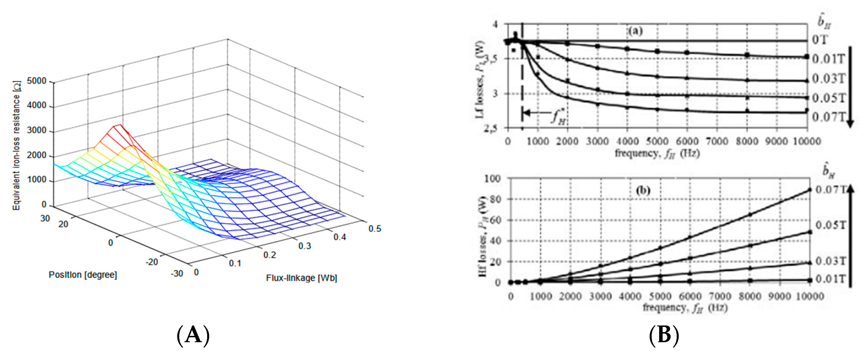
Nonetheless, these studies face limitations due to the applicability of iron power loss formulas predominantly only at very low frequencies [16]. The maximum studied frequency was often in tenths of a kilohertz, which is not applicable to broad harmonic signals, as shown in Figure 2.

Moreover, these determination methods require specific expensive equipment, such as a sinusoidal variable frequency power supply and the corresponding sensors, in order to perform the necessary measurements. The frequency range that the power supply can provide is also a limiting factor and is often the reason why the maximum frequency studied is so low. These methods properly check how different frequencies affect iron losses because their sensors only work well at low frequencies. They are unable to show which frequency ranges cause the most energy loss in the electromagnetic and magnetic device. As a result, they do not give the full picture of iron losses under real, varied conditions.

2.2. First Resonance Frequency Measurement

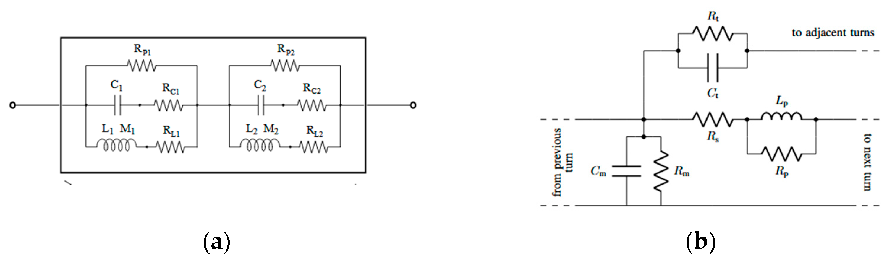
The conventional technique associates the determination of the resistance of iron losses with impedance measurements performed at the first resonance frequency of the device.

Toudji et al. and Grandi et al. have used this type of circuit model, which is equivalent to the low to medium frequency in Figure 3 [11,23].

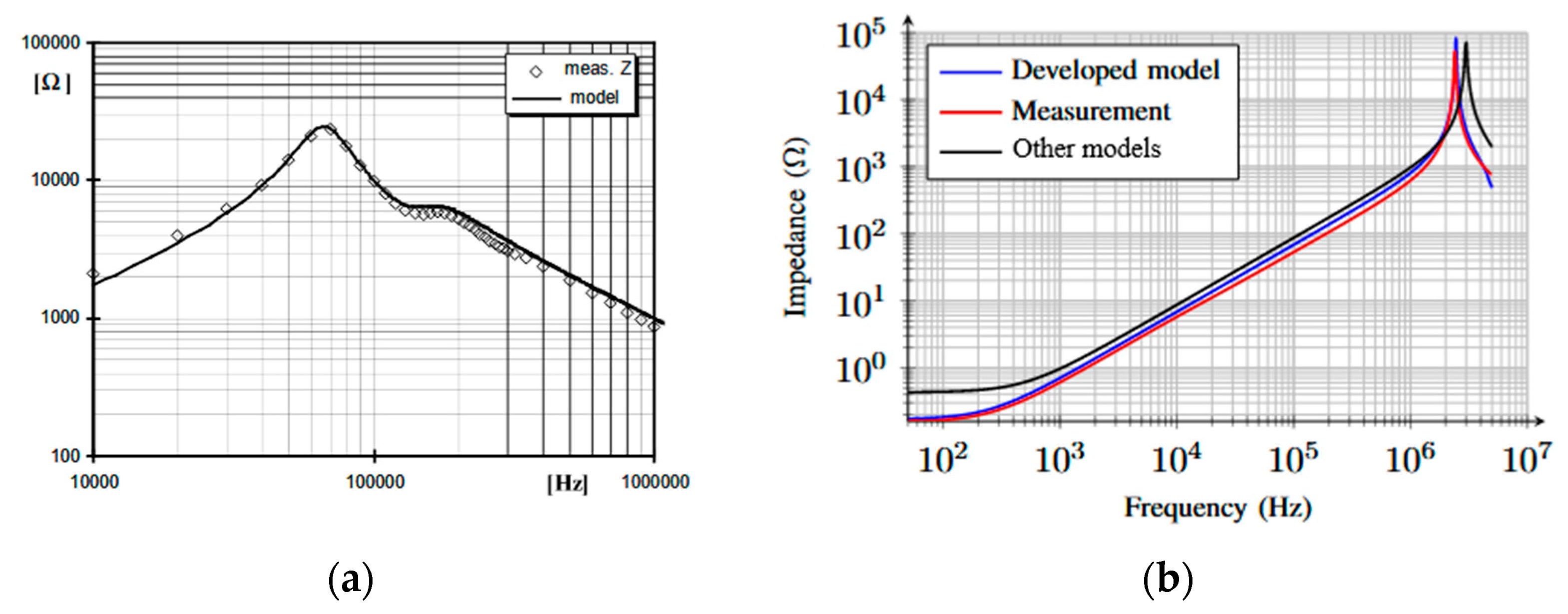
Using an impedance analyzer such as the HP4300 series from Agilent Technologies, Santa Clara, CA, USA, they extracted the impedance measurements of their respective devices. They then fixed the iron loss equivalent resistance value called “Rp” in their figure directly to the measured impedance value at the first frequency resonance, as shown if Figure 4.

Although this method is widely accepted for its simplicity, it presumes a constancy of resistance beyond this frequency, which may not be relevant for some devices operating under complex dynamic regimes or exposed to atypical conditions, such as high levels of saturation or magnetic disturbances [6,11,23].

2.3. Complex Magnetic Permeability

The extraction of resistance through complex magnetic permeability offers another alternative. Examples of use of this method have been provided by Ruiz-Sarrio et al. and Cuellar et al. [7,15,24].

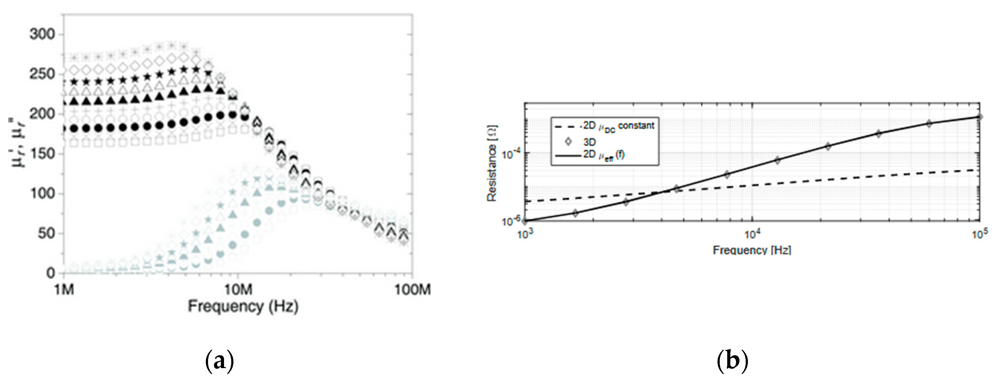
In their papers, the authors present the same method of determination. First, they calculate the relative magnetic permeability of their magnetic devices under DC conditions. Further calculations then transform this into complex frequency-dependent magnetic permeability, taking into account the eddy currents within the laminations of the magnetic device. The imaginary part of this complex magnetic permeability is then used to determine the equivalent resistance of iron losses, as shown in Figure 5.

The limiting factor of this method is the fact that the complex magneticity does not consider the hysteresis effect affecting the magnetic device, which contributes to the nonlinearity [15]. Furthermore, an impedance measurement can also be used to extract the complex magnetic permeability in some cases, adding to the criticism in Section 2.2 [15]. Because of this, the results may not match real performance, making them less useful for designing and modeling actual devices.

2.4. Limits of These Methods

The existing methods have certain limitations, as they do not fully represent the real operating conditions of electromagnetic and magnetic devices. For example, measuring the first resonance frequency at low signal levels does not account for important effects such as magnetic saturation and hysteresis. Additionally, calculations of complex magnetic permeability—which are used to estimate the iron loss equivalent resistance—are often based on simplifying assumptions. These assumptions usually ignore the effects of hysteresis.

For these reasons, we propose an experimental measurement approach that takes all of these physical effects into account. This method should allow a more precise measurement that the impedance analyzer in a respectable amount of time.

3. Measurement and Estimation Method

This method is based on the evaluation of the complex impedance of a magnetic device fed with a switching power supply corresponding to an operating point. Then, a rich, harmonics-broadband voltage signal will excite the magnetic device.

3.1. Method Description

To analyze the frequency response near the nominal operating point, the wound device is supplied using a voltage pulse characterized by a low duty cycle to ensure a broad harmonic spectrum.

The method’s effectiveness is demonstrated through a MATLAB Simulink 2022b simulation featuring a circuit with constants such as copper resistance, inductance, and iron loss equivalent resistance, shown in Figure 1, given in the Section 1. A voltage pulse generator supplies the circuit, operating at 500 V amplitude, 10 kHz frequency, and a 2% duty cycle, as summarized in

Table 1. Parameters of the pulse generator.

Parameters	Values
Voltage amplitude	500 V
Frequency	10 kHz
Duty cycle of the pulse	2%

.

In this simulation, the parameters are fixed with the copper resistance ${\mathrm{R}}_{\mathrm{copper}} = 2 \mathsf{\Omega }$, the inductance $\mathrm{L} = 1 \mathrm{mH},$and the equivalent iron loss resistance ${\mathrm{R}}_{\mathrm{iron}} = 5000 \mathsf{\Omega }$.

Voltage and current steady-state periods are recorded at a fixed time step, determined by the desired maximum observable frequency, complying with the Shannon–Nyquist principle [26]. For this simulation, the time step is set at 1 ns, with data acquisition starting after reaching steady state.

In MATLAB, the signals are processed with the Fast Fourier Transform (FFT). From the Fourier series coefficients, impedance and phase values at corresponding frequencies are extracted.

The Fast Fourier Transform (FFT) is applied to the voltage and current signals as follows:

$$\mathrm{v}\left(\mathrm{t}\right)= \sum _{\mathrm{n}=0}^{\infty }{\mathrm{V}}_{\mathrm{n}}{\mathrm{e}}^{-\mathrm{jn}\mathrm{\omega }\mathrm{t}}$$

(1)

$$\mathrm{i}\left(\mathrm{t}\right)=\sum _{\mathrm{n}=0}^{\infty }{\mathrm{I}}_{\mathrm{n}}{\mathrm{e}}^{-\mathrm{jn}\mathrm{\omega }\mathrm{t}}$$

(2)

where ${\mathrm{V}}_{\mathrm{n}}$, ${\mathrm{I}}_{\mathrm{n}}$ is the Fourier series complex coefficient of rank n, $\mathrm{\omega } = 2\mathrm{\pi }{\mathrm{f}}_1$, and ${\mathrm{f}}_1$ is the fundamental frequency of the supplied periodic pulse voltage.

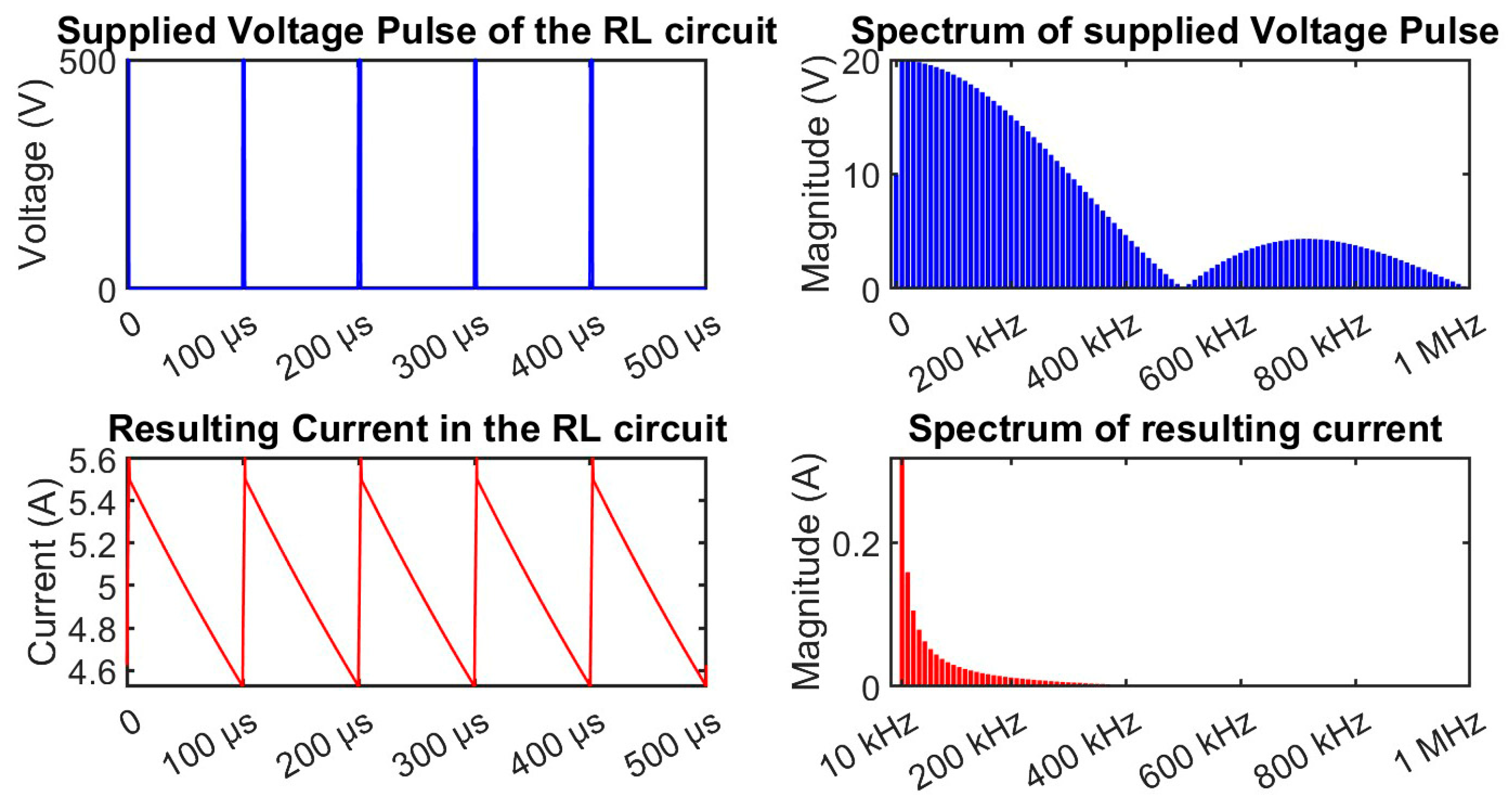
The time signals and spectra are shown in Figure 6. In order to facilitate the display of the current spectrum, the DC component is removed from the spectrum graph. The value of the DC component of the current is 5.0 A.

From the coefficients ${\mathrm{V}}_{\mathrm{n}}$ and ${\mathrm{I}}_{\mathrm{n}}$, the values of the impedance Z and the phase φ of the circuit are determined at the corresponding frequencies:

$$\mathrm{Z}\left({\mathrm{f}}_{\mathrm{n}}\right) = \mathrm{Z}\left(\mathrm{n}{\mathrm{f}}_1\right) ={\mathrm{V}}_{\mathrm{n}}/{\mathrm{I}}_{\mathrm{n}}$$

(3)

$$\mathrm{\phi }\left({\mathrm{f}}_{\mathrm{n}}\right)=\arg \left( \mathrm{Z}\left({\mathrm{f}}_{\mathrm{n}}\right)\right)$$

(4)

Depending on the supply voltage signal, such as a pulse, the corresponding spectrum may contain harmonics with a magnitude close to zero, as shown in Figure 7. Digital processing may be required to prevent divergence in impedance calculations with these particular harmonics, such as a direct thresholding on the magnitude of the harmonics. Such methods are employed and explained by Creux et al. [27].

The resulting impedance modulus and phase are obtained in Figure 8. The fundamental frequency fixes the lowest observable value of the impedance.

3.2. Theoretical Determination of the Iron Loss Equivalent Resistance

Electrical equations of the circuit model in Figure 1 from the “Introduction” Section lead to the equivalent impedance Z:

$$\mathrm{Z} ={\displaystyle \frac{{\mathrm{R}}_{\mathrm{copper}}{\mathrm{L}}^2{\mathrm{\omega }}^2 +{ \mathrm{R}}_{\mathrm{copper}}{\mathrm{R}}_{\mathrm{iron}}^2 + {\mathrm{L}}^2{\mathrm{\omega }}^2{\mathrm{R}}_{\mathrm{iron}}}{{\mathrm{L}}^2{\mathrm{\omega }}^{2 }+{ \mathrm{R}}_{\mathrm{iron}}^2}} + \mathrm{j}{\displaystyle \frac{{\mathrm{R}}_{\mathrm{iron}}^2\mathrm{L}\mathrm{\omega }}{{\mathrm{L}}^2{\mathrm{\omega }}^2 + {\mathrm{R}}_{\mathrm{iron}}^2}}$$

(5)

The real and imaginary part of the impedance ((6) and (7)) can be used to determine ${\mathrm{R}}_{\mathrm{iron}}$.

$$\mathrm{Re}\left(\mathrm{Z}\right)={\displaystyle \frac{{\mathrm{R}}_{\mathrm{copper}}{\mathrm{L}}^2{\mathrm{\omega }}^{2 }+{\mathrm{R}}_{\mathrm{copper}}{\mathrm{R}}_{\mathrm{iron}}^2+{\mathrm{R}}_{\mathrm{iron}}{\mathrm{L}}^2{\mathrm{\omega }}^2}{{\mathrm{L}}^2{\mathrm{\omega }}^{2 }+{\mathrm{R}}_{\mathrm{iron}}^2}}$$

(6)

$$\mathrm{Im}\left(\mathrm{Z}\right)={\displaystyle \frac{{\mathrm{R}}_{\mathrm{iron}}^2\mathrm{L}\mathrm{\omega }}{{\mathrm{L}}^2{\mathrm{\omega }}^2+{\mathrm{R}}_{\mathrm{iron}}^2}}$$

(7)

From Im(Z), the expression of ${\mathrm{R}}_{\mathrm{iron}}^2$ can be found in Equation (8):

$${\mathrm{R}}_{\mathrm{iron}}^2 = {\displaystyle \frac{\mathrm{Im}\left(\mathrm{Z}\right){\mathrm{L}}^2{\mathrm{\omega }}^2}{\mathrm{L}\mathrm{\omega } - \mathrm{Im}\left(\mathrm{Z}\right)}}$$

(8)

From Re(Z), the expression of ${\mathrm{L}}^2$can be found in Equation (9):

$${\mathrm{L}}^2 = {\displaystyle \frac{1}{{\mathrm{\omega }}^2}}.{\displaystyle \frac{{\mathrm{R}}_{\mathrm{fer}}^2(\mathrm{Re}\left(\mathrm{Z}\right)- {\mathrm{R}}_{\mathrm{s}})}{{\mathrm{R}}_{\mathrm{s}}+{\mathrm{R}}_{\mathrm{fer}} - \mathrm{Re}\left(\mathrm{Z}\right)}}$$

(9)

The following expression for ${\mathrm{R}}_{\mathrm{iron}}$ is obtained:

$${\mathrm{R}}_{\mathrm{iron}} ={\displaystyle \frac{{\left(\mathrm{Re}\left(\mathrm{Z}\right) - {\mathrm{R}}_{\mathrm{copper}}\right)}^2+{\mathrm{Im}\left(\mathrm{Z}\right)}^2}{\left(\mathrm{Re}\left(\mathrm{Z}\right) - {\mathrm{R}}_{\mathrm{copper}}\right)}}$$

(10)

This result is independent of the inductance L but depends on the resistance ${\mathrm{R}}_{\mathrm{copper}}$.

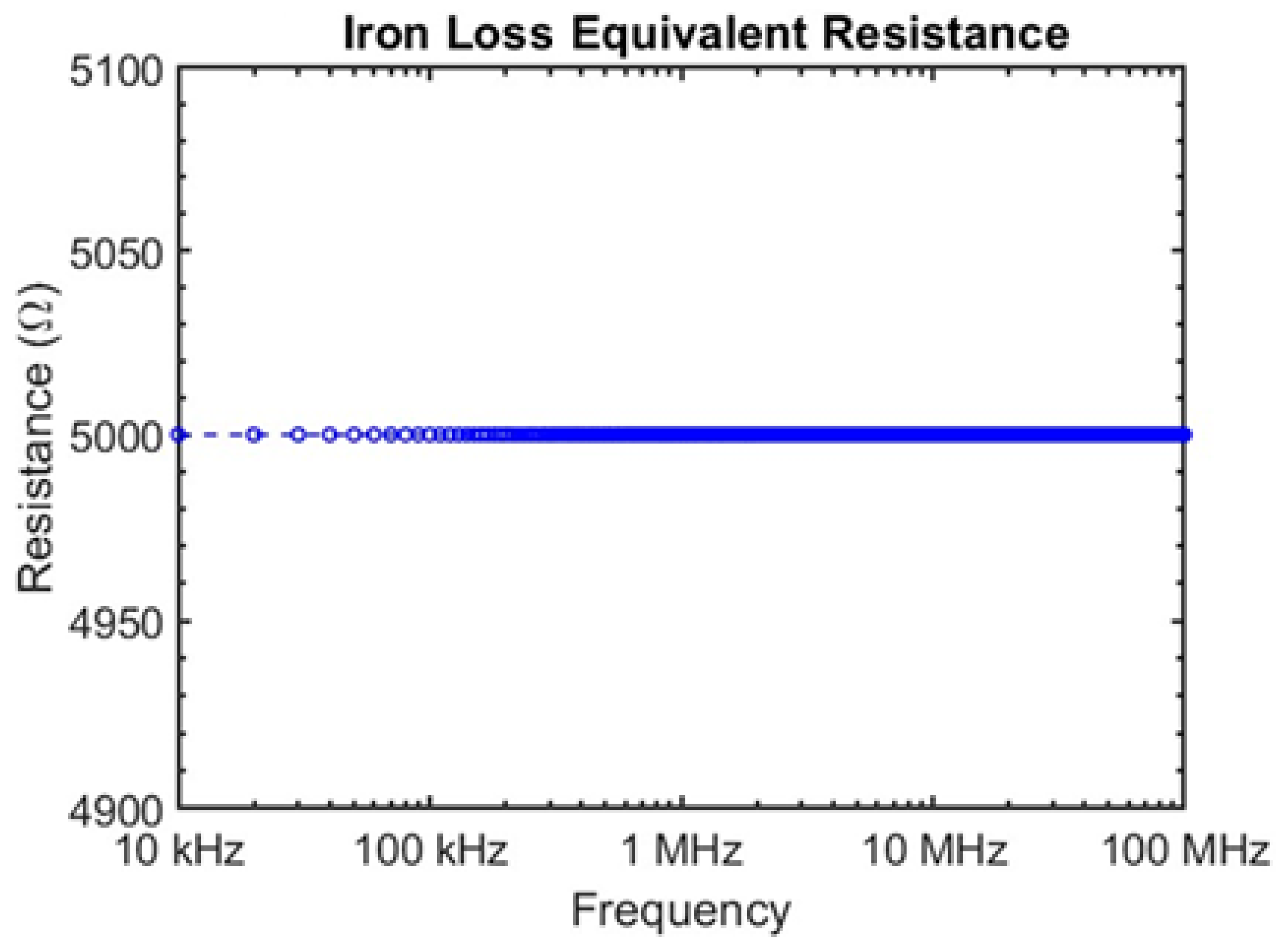
In the case of our example and simulation, the following ${\mathrm{R}}_{\mathrm{iron}}$ is obtained with a constant ${\mathrm{R}}_{\mathrm{copper}} = 2 \mathsf{\Omega }$ in Figure 9.

By applying the method in simulation, it is possible to obtain the value of ${\mathrm{R}}_{\mathrm{iron}}$ for different frequencies.

The iron loss equivalent resistance can only be determined at the frequencies present in the voltage pulse spectrum, provided that the copper resistance is known and the real and imaginary parts of the impedance are indirectly obtained from the measurements.

In most of the cases, the geometry of the wound devices is known, so ${\mathrm{R}}_{\mathrm{copper}}$ values can be determined by using finite element method, considering skin and proximity effects.

4. Experimental Results

In order to apply the method, an experimental measuring test bench has been constructed with adapted sensors and the corresponding power supply.

To enable comparison, impedance measurements have been carried out using a T3LCR1100 impedance analyzer, from TeledyneLeCroy, Loomis, CA, USA.

4.1. Measurement Setup and Data Processing

The measurement setup consists of a DC power voltage supply with a maximum voltage of 600 V and a maximum current of 8.5 A. It is connected to a half inverter leg. The switch T1 is controlled by DSPACE, which allows it to be controlled at the desired frequency and duty cycle. The wound device is connected to the T2 switch directly, which is not driven. A schematic of the setup is shown in Figure 10.

The voltage is measured at the wound device terminals by a passive voltage probe with a 400 MHz bandwidth, from Lecroy, USA. The current is also measured at the wound device terminals by a RT-ZC20 Probe with an RT-ZA13 Amplifier, both from Rohdes & Schwarz, Munich, Germany, having a bandwidth of 100 MHz. Finally, the signals are visualized and recorded on a MS046 scope, from Tektronix, Beaverton, OR, USA, with a bandwidth of 600 MHz. Details are available in

Table 2. Equipment used in the setup.

Equipment	Name	Relevant Parameters
Power Supply	GEN600-8.5, from TDK-Lambda, Achern, Germany	DC Voltage: 0–600 V DC Amps: 0–8.5 A
Scope	MSO46, from Tektronix, Beaverton, OR, USA	Bandwidth: 600 MHz Sample Rate: 10 GS/s
Voltage Sensor	Lecroy PPE 2 KV, from Lecroy, Chestnut Ridge, NY, USA	Bandwidth: 400 MHz Input Capacitance: <6 pF Attenuation: 1:100
Current Sensor	RT-ZC20 Probe + RT-ZA13 Amplifier, from Rohde & Schwarz, Munich, Germany	Bandwidth: 100 MHz Propagation Delay: 17 ns Sensitivity Range: 1 A/V–10 A/V
Thermal Camera	T200, from FLIR, Wilsonville, OR, USA	Temperature Range: −20 °C–1200 °C

.

In this experimental configuration, the wound device consists of a coil composed of 48 copper turns, located around a magnetic core made from NO20 Fe-Si laminated sheets, from Isolectra, Estrées-Deniécourt, France. The system is configured with a sampling frequency of 3.125 GHz. Pulse generation is achieved through the switching states of T1.

Synchronization of the oscilloscope with T1’s control signal enables accurate acquisition of voltage and current signals flowing through the winding over a complete period. To mitigate acquisition noise inherent to the experimental setup, the averaging function of the oscilloscope is employed, allowing signal filtering without inducing phase shifts. Subsequently, the data is converted into MATLAB format.

During data processing, compensation for the 17 ns propagation delay, as detailed in Table 1, associated with the current probe and its amplifier, is necessary. The final data processing workflow aligns with the procedures outlined in Section 1. This methodology facilitates the estimation of various ${\mathrm{R}}_{\mathrm{iron}}$ values corresponding to different operational points, utilizing the approach delineated in Section 1.

4.2. Measurement Results

These operating points are representative of the operating point of the coils in a DC–DC converter.

4.2.1. Results and Comparison

Two set of measurements are realized on the test bench in Figure 11. They are performed with the settings given in

Table 3. Setting of the acquisition.

Parameters	Operating Point 1	Operating Point 2
Voltage amplitude	50 V	120 V
Frequency	5 kHz	5 kHz
Duty cycle of the pulse	1.6%	1.6%
Current DC component	300 mA	1.4 A

. Voltage and current acquisitions are displayed in Figure 12 for operating point 2.

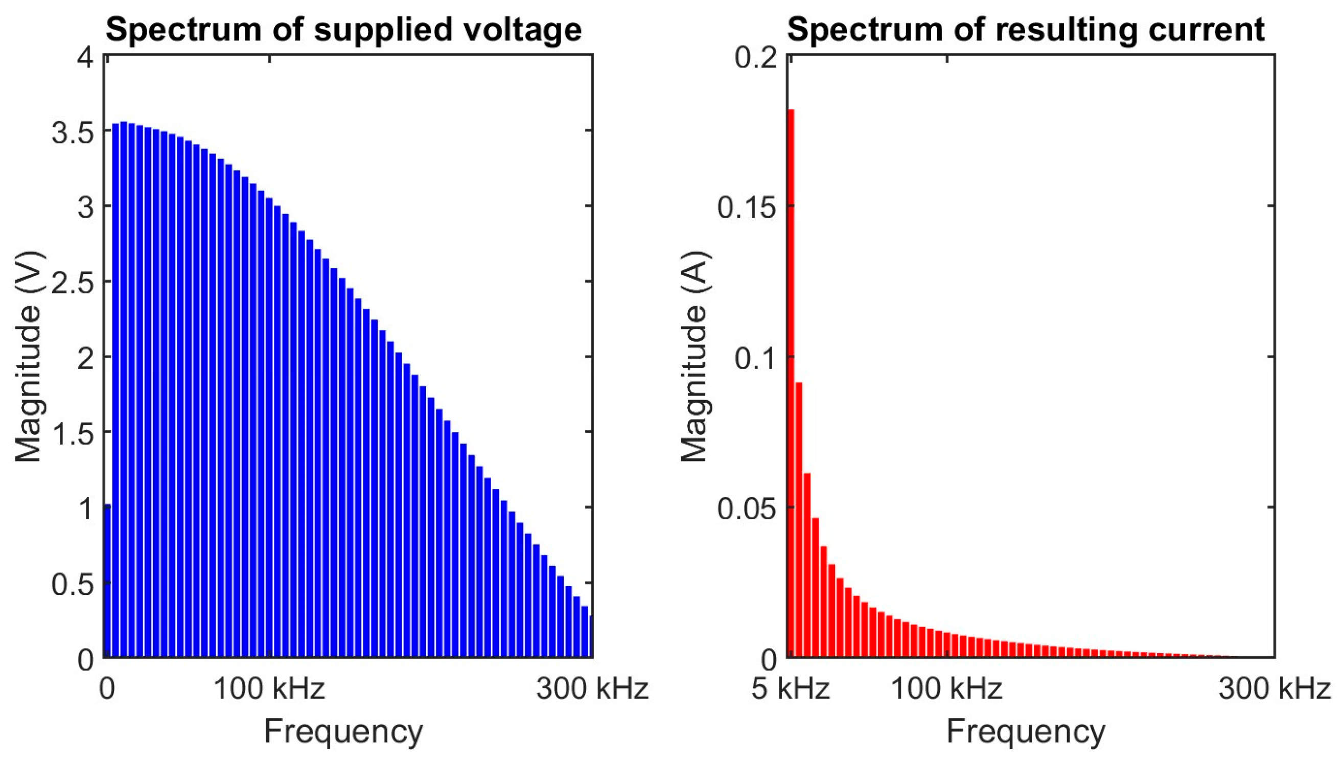
The ensuing spectra as well as impedance and phase diagrams are available, respectively, in Figure 13 and Figure 14. DC component of the current spectrum is removed from the display and is equal to 1.4 A.

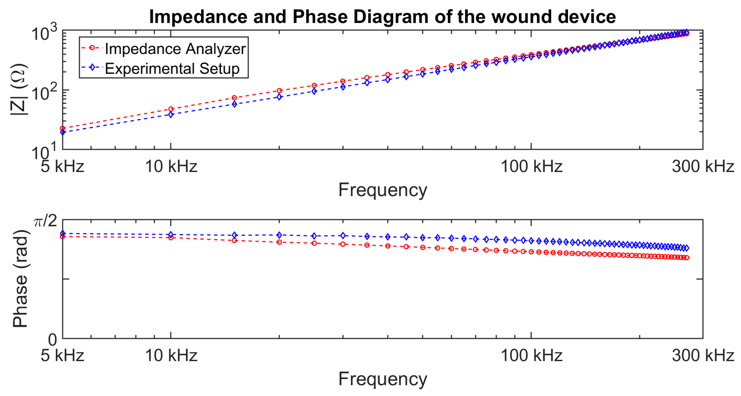
Impedance and phase obtained from the method developed in Section 1 and from the T3LCR1100 Impedance Analyzer, from TeledyneLecroy, Loomis, CA, USA are compared in Figure 14.

By analyzing the impedance and phase diagrams for each method, the difference is obvious. At this point, we can conclude that the operating point has an impact on the low- to medium-frequency behavior of the wound device.

The estimated parameters related to the equivalent circuit of wound devices (Figure 1) will be different depending on the measurement method.

In this paper, we focus our attention on the evaluation of the iron loss equivalent resistance (${\mathrm{R}}_{\mathrm{i}\mathrm{r}\mathrm{o}\mathrm{n}}$). As seen in Equation (8), it is possible to estimate ${\mathrm{R}}_{\mathrm{i}\mathrm{r}\mathrm{o}\mathrm{n}}$ with the knowledge of the complex impedance and the copper resistance (${\mathrm{R}}_{\mathrm{c}\mathrm{o}\mathrm{p}\mathrm{p}\mathrm{e}\mathrm{r}}$).

4.2.2. Determination of Copper Resistance

As stated previously, determining the value of the copper resistance is required to calculate the iron loss equivalent resistance.

In our case, a 2D finite element model with finite element software GetDp Version 3.30 of the wound device is used that takes into account frequency-dependent effects such as skin and proximity effects [28].

The conductivity of copper is set to the controlled temperature of 26 °C, which is the temperature at which previous measurements were conducted. The temperature measurement was carried out using a thermal camera directly pointed toward the magnetic device.

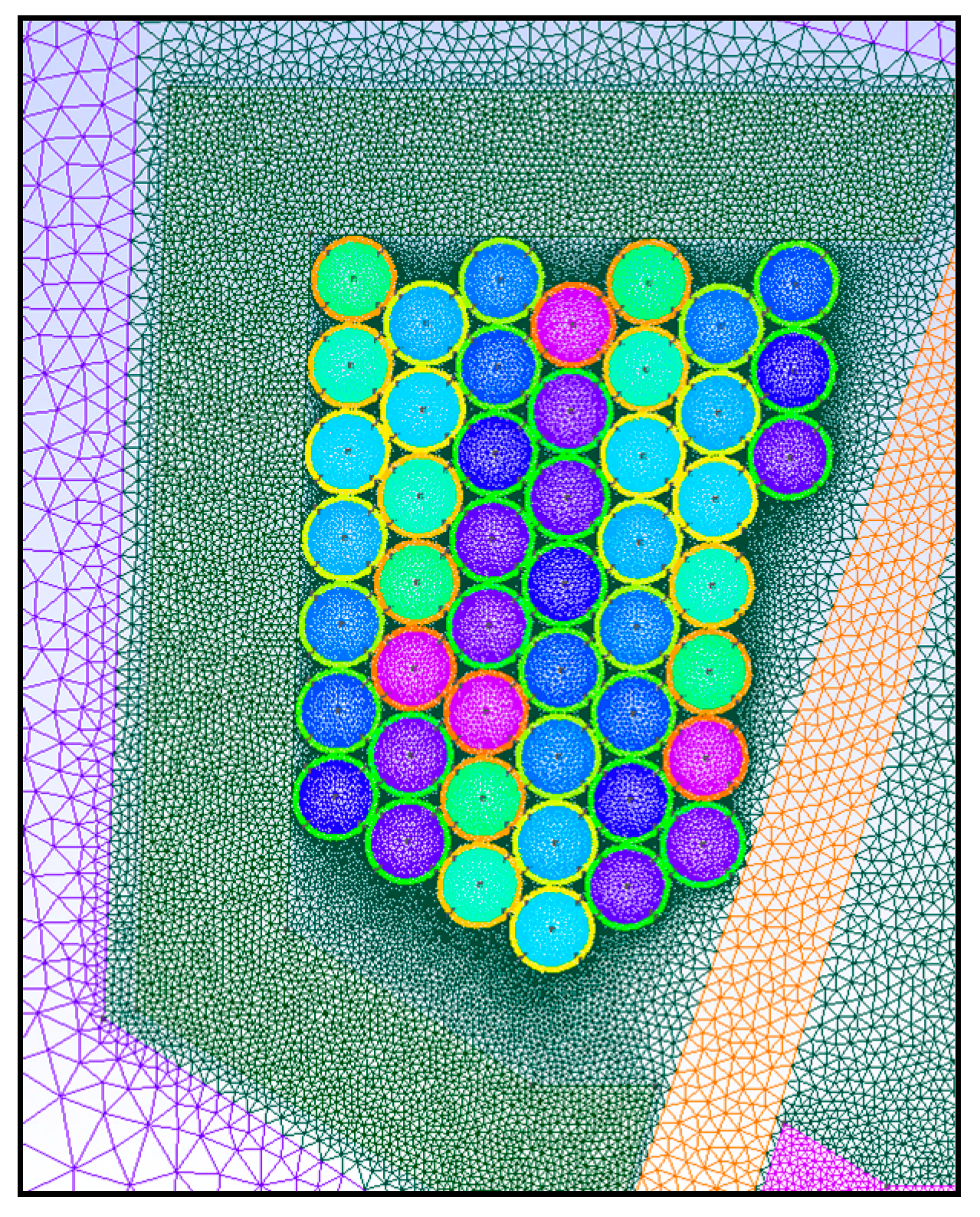
The finite element software, showcased in Figure 15, calculates the equivalent copper resistance ${\mathrm{R}}_{\mathrm{c}\mathrm{o}\mathrm{p}\mathrm{p}\mathrm{e}\mathrm{r}}$ of the wound device for the frequencies of the harmonic content of the voltage pulse.

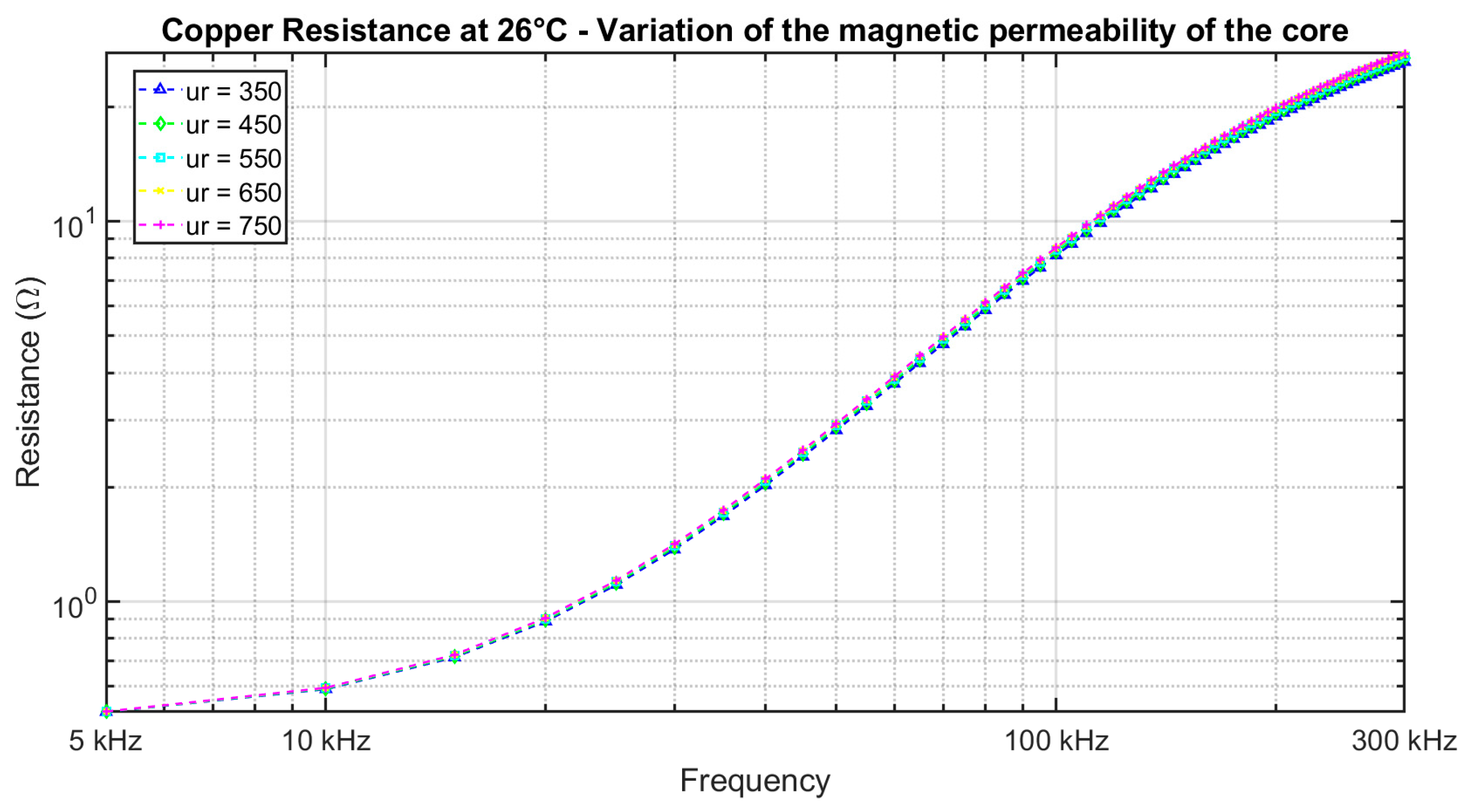
As reported in other studies, the magnetic permeability ${\mathrm{\mu }}_{\mathrm{r}}$ function decreases as the frequency increases [29].

The apparent permeability of conductive magnetic materials, such as Fe-Si steel, decreases rapidly at higher frequencies due to increased eddy current losses [30,31]. Variations in ${\mathrm{R}}_{\mathrm{copper}}$ depending of the relative magnetic permeability of the magnetic core ${\mathrm{\mu }}_{\mathrm{r}}$ in the wound device are shown in Figure 16.

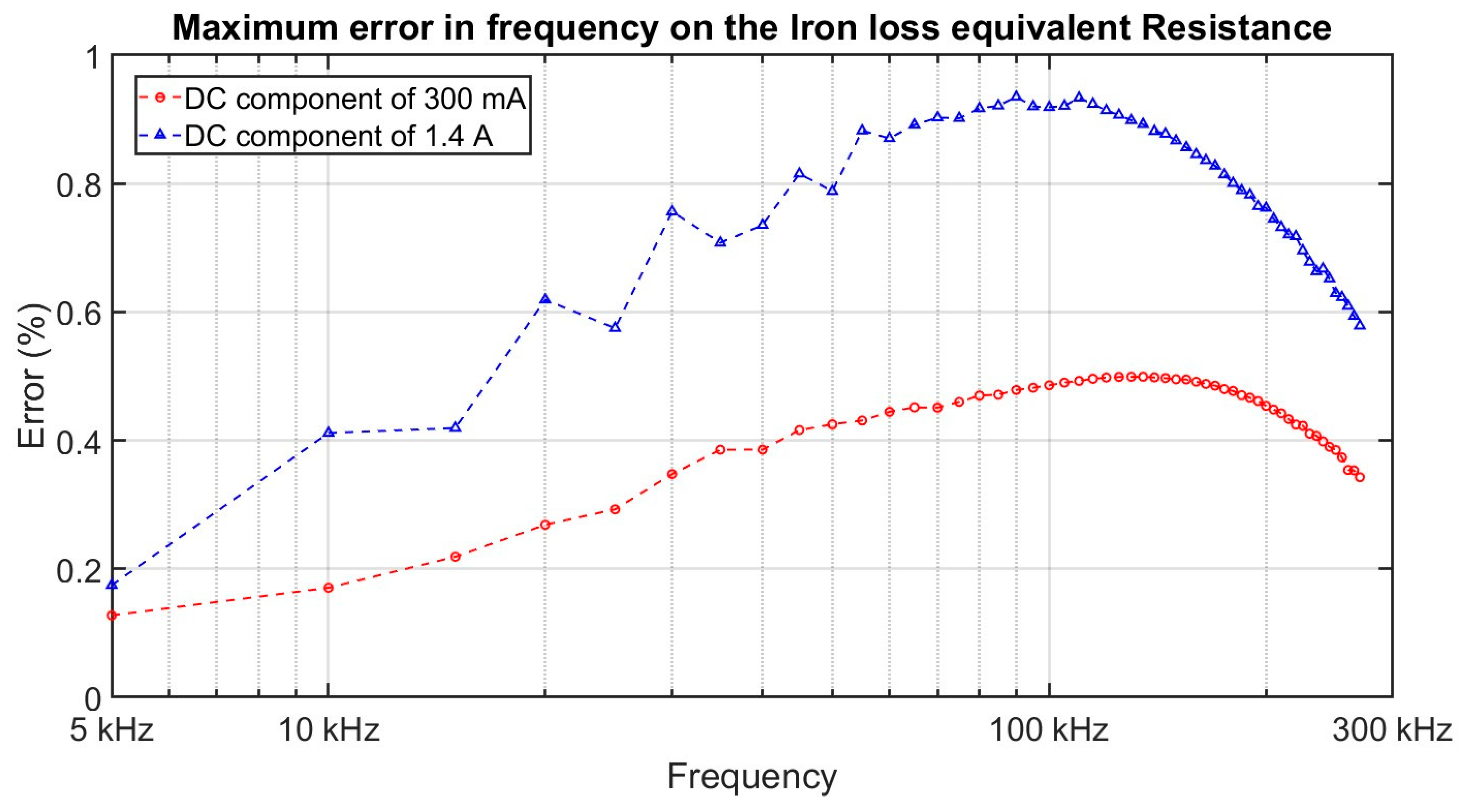
In this frequency range, ${\mathrm{R}}_{\mathrm{copper}}$ varies slightly and only affects the result of the iron loss equivalent resistance by less than 1% (Figure 17) with the lowest magnetic permeability. Our results are thus only slightly affected by the variation in the magnetic permeability.

4.3. Determination of the Iron Loss Equivalent Resistance

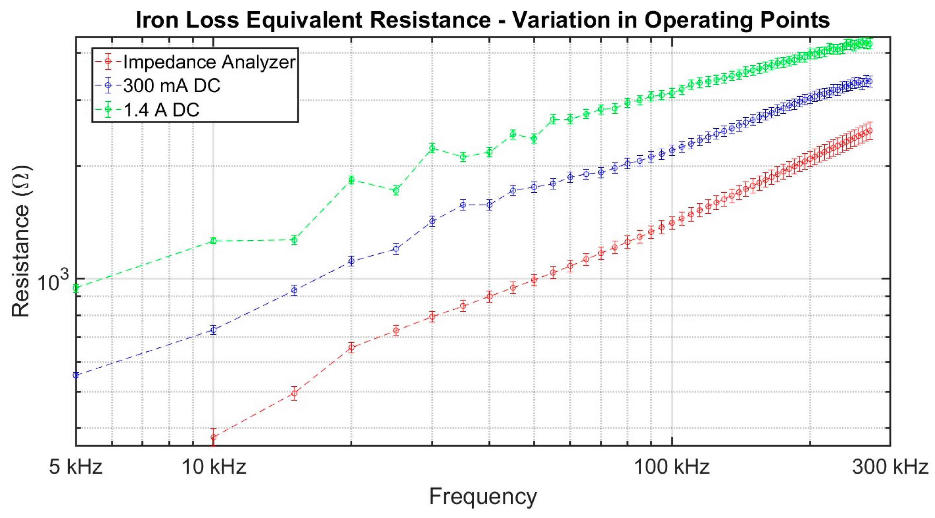
The iron loss equivalent resistance calculated according to the steps in Section 2.2 and the impedance analyzer are compared at Figure 18. Thermal steady state at 26 °C is ensured before signal acquisition, and determination of the copper resistance is also performed at 26 °C.

The sensitivity errors associated with the voltage and current sensors were taken into account, estimated at 2% and 3%, respectively. Numerical errors originating from the oscilloscope were also considered, but these were found to be negligible in comparison to the sensor errors.

A frequency dependence of the iron loss equivalent resistance is visualized, while also being dependent on the operating point at which the magnetic device is running. It validates the influence of the operating point on the evaluation of the iron loss equivalent resistance.

5. Discussion

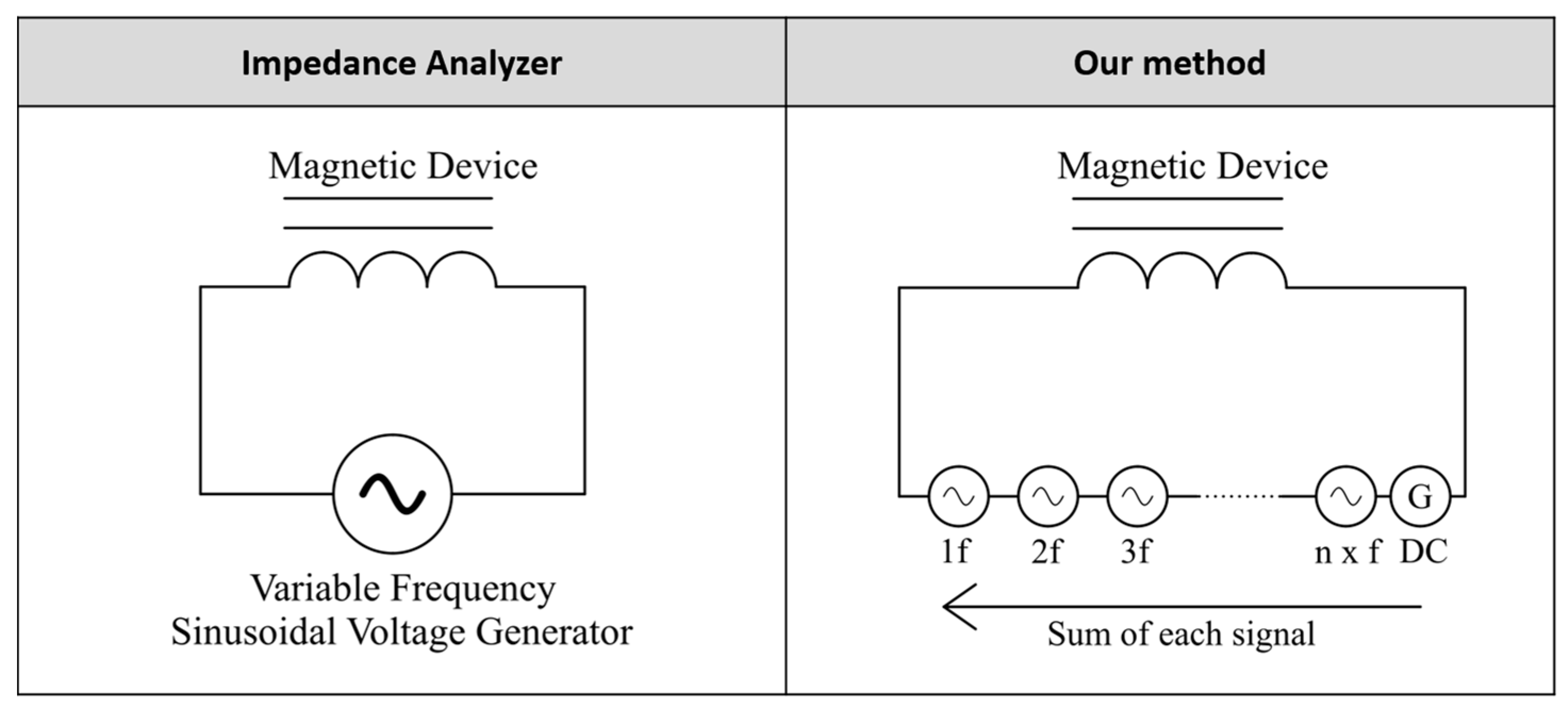
The differences between our measurement approach and the one implemented with conventional impedance analyzers can largely be attributed to the nonlinear behavior exhibited by electromagnetic or magnetic devices. A key phenomenon explaining this difference is harmonic intermodulation. In a traditional impedance analyzer, only the fundamental component of the current, resulting from a perfectly sinusoidal voltage input, is taken into account in the measurement process, shown in Figure 19.

By contrast, in our case, the nonlinear electromagnetic or magnetic device is subjected to voltage excitations containing numerous harmonics. This excitation generates an even higher number of current harmonics at the output, which significantly affects impedance determination. The generated current harmonics may add to or subtract from the existing ones, influencing the resulting signal and impedance determination.

In addition to this limitation, another physical phenomenon characteristic of magnetic materials, particularly of the ferromagnetic type, comes into play: the existence of minor hysteresis loops. Minor hysteresis loops are smaller cycles that develop around the major loop formed by the fundamental excitation component in an electromagnetic or magnetic device. According to Petrea et al., the presence of these minor loops around the major one leads to a reduction in both the material’s dynamic coercivity and—most notably—its permeability, especially at high frequencies [21].

Further, Petrea et al.’s research demonstrates that high-frequency harmonic content directly impacts the low-frequency behavior of the device, establishing a clear link between the effects of minor loops and the methods used to measure the impedance of electromagnetic and magnetic devices. As a result, changes in magnetic properties in the presence of harmonic content influence not only the determination of the material’s impedance but also our estimation of its equivalent iron loss resistance [21].

Finally, because the frequency sweep in an impedance analyzer is performed with a purely sinusoidal power supply, such an analyzer is fundamentally incapable of generating and exciting an electromagnetic or magnetic device in a manner that would give rise to minor hysteresis loops. This means that conventional impedance analyzers cannot capture these essential dynamic effects, resulting in measurement limitations when characterizing nonlinear magnetic materials under realistic, harmonic-rich excitation conditions.

In summary, by explicitly considering the effects of minor hysteresis loops and harmonic intermodulation, our method offers a more precise and realistic determination of iron loss equivalent resistance under real operating conditions, including phenomena such as electromagnetic and magnetic saturation. This approach is unique because it accounts for the actual dynamic behavior of magnetic devices under complex excitation, which traditional methods typically overlook. As a result, our methodology provides data that is not only more accurate but is also directly applicable to the modeling and design of advanced electromagnetic components. Such improved precision is particularly valuable for high-frequency transformers, power electronics, and other applications where understanding complex magnetic behavior is critical. This makes our results significantly more suitable and relevant for both detailed circuit modeling and the further development of next-generation electromagnetic and magnetic devices.

6. Conclusions

This work began by reviewing the development of measurement techniques for electromagnetic and magnetic devices, focusing on the challenges of characterizing iron loss equivalent resistance under realistic operating conditions. The state of the art highlights the growing importance of evaluating devices directly under their typical working points, especially as modern applications increasingly rely on complex, harmonic-rich excitations.

We have introduced a novel method for determining the iron loss equivalent resistance of magnetic devices directly at their actual operating point. This method involves exciting the magnetic device with a voltage signal rich in harmonics and measuring both this voltage and the resulting current. Using these measurements, the complex impedance of the winding can be directly determined through FFT (Fast Fourier Transform) analysis. This approach consists of three essential elements: accurate measurement during operation, careful calibration of the sensors to ensure reliable data, and dedicated digital processing to extract the relevant parameters from the measurements. Each of these steps contributes to the accuracy and repeatability of the method.

The method was successfully implemented on an electromagnetic device, confirming its practical viability. As an example of the results in Figure 18, at 10 kHz, the estimated iron loss equivalent resistance for a 1.4 A DC operating point is 1262 Ω ± 23 Ω, while for a 300 mA DC operating point, it is 731 Ω ± 21 Ω. For comparison, the value obtained with the impedance analyzer is 378 ± 20 Ω. This represents a difference of approximately 333% between the 1.4 A DC operating point and the impedance analyzer and about 193% for the 300 mA DC case. The study demonstrates that the DC component of the current has a clear impact on the impedance of electromagnetic devices and therefore on the iron loss equivalent resistance. This underlines the relevance and the importance of our method in applications where the operating currents may deviate from purely alternating forms.

A fundamental difference between our method and traditional impedance analyzer measurements can be attributed to the consideration of intermodulation effects and the complex magnetic phenomena known as minor loops. Unlike conventional techniques, our method takes into account these nonlinear effects, which results in a more accurate and comprehensive assessment.

To our knowledge, this practical measurement technique is not yet standard in the field, but it offers significant flexibility and adaptability. It can be applied to a wide range of electromagnetic and magnetic devices for the direct measurement of iron loss equivalent resistance, which is highly valuable for device design and optimization. Looking ahead, the method will be extended to analyze performance under various supply waveforms, including Pulse-Width Modulation (PWM). In particular, this includes validating the technique with multilevel PWM signals and in scenarios involving high switching frequencies—such as those found in advanced inverters equipped with Gallium Nitride (GaN) components driving electrical motors. These systems are increasingly common due to their high efficiency and ability to operate at very high switching speeds.

Overall, this method offers a reliable and innovative solution for characterizing iron loss equivalent resistance under realistic operating conditions. It paves the way for further research and development, making it particularly relevant for the measurement and design of next-generation magnetic components used in modern power electronic systems.

References

- Ding, N.; Prasad, K.; Lie, T.T. The Electric Vehicle: A Review. Int. J. Electr. Hybrid Veh. 2017, 9, 49. [Google Scholar] [CrossRef]
- Sarlioglu, B.; Morris, C.T. More Electric Aircraft: Review, Challenges, and Opportunities for Commercial Transport Aircraft. IEEE Trans. Transp. Electrif. 2015, 1, 54–64. [Google Scholar] [CrossRef]
- Polinder, H.; Ferreira, J.A.; Jensen, B.B.; Abrahamsen, A.B.; Atallah, K.; McMahon, R.A. Trends in Wind Turbine Generator Systems. IEEE J. Emerg. Sel. Top. Power Electron. 2013, 1, 174–185. [Google Scholar] [CrossRef]
- Wei, M.; McMillan, C.A.; de la Rue du Can, S. Electrification of Industry: Potential, Challenges and Outlook. Curr. Sustain. Renew. Energy Rep. 2019, 6, 140–148. [Google Scholar] [CrossRef]
- Magdun, O.; Blatt, S.; Binder, A. Calculation of Stator Winding Parameters to Predict the Voltage Distributions in Inverter Fed AC Machines. In Proceedings of the 2013 9th IEEE International Symposium on Diagnostics for Electric Machines, Power Electronics and Drives (SDEMPED), Valencia, Spain, 27–30 August 2013; pp. 447–453. [Google Scholar]
- Toudji, M.; Parent, G.; Duchesne, S.; Dular, P. Determination of Winding Lumped Parameter Equivalent Circuit by Means of Finite Element Method. IEEE Trans. Magn. 2017, 53, 9401904. [Google Scholar] [CrossRef]
- Ruiz-Sarrio, J.E.; Chauvicourt, F.; Gyselinck, J.; Martis, C. Impedance Modeling Oriented Toward the Early Prediction of High-Frequency Response for Permanent Magnet Synchronous Machines. IEEE Trans. Ind. Electron. 2023, 70, 4548–4557. [Google Scholar] [CrossRef]
- Memon, A.A.; Bukhari, S.S.H.; Ro, J.-S. Experimental Determination of Equivalent Iron Loss Resistance for Prediction of Iron Losses in a Switched Reluctance Machine. IEEE Trans. Magn. 2022, 58, 8102404. [Google Scholar] [CrossRef]
- Hajji, T.E.; Hlioui, S.; Louf, F.; Gabsi, M.; Belahcen, A.; Mermaz-Rollet, G.; Belhadi, M. AC Losses in Windings: Review and Comparison of Models With Application in Electric Machines. IEEE Access 2024, 12, 1552–1569. [Google Scholar] [CrossRef]
- Zhu, S.; Shi, B. Modeling of PWM-Induced Iron Losses With Frequency-Domain Methods and Low-Frequency Parameters. IEEE Trans. Ind. Electron. 2022, 69, 2402–2413. [Google Scholar] [CrossRef]
- Grandi, G.; Kazimierczuk, M.K.; Massarini, A.; Reggiani, U.; Sancineto, G. Model of Laminated Iron-Core Inductors for High Frequencies. IEEE Trans. Magn. 2004, 40, 1839–1845. [Google Scholar] [CrossRef]
- Mahdavi, S.; Hameyer, K. High Frequency Equivalent Circuit Model of the Stator Winding in Electrical Machines. In Proceedings of the 2012 XXth International Conference on Electrical Machines, Marseille, France, 2–5 September 2012; pp. 1706–1711. [Google Scholar]
- Mombello, E.E. Impedances for the Calculation of Electromagnetic Transients within Transformers. IEEE Trans. Power Deliv. 2002, 17, 479–488. [Google Scholar] [CrossRef]
- Suresh, G.; Toliyat, H.A.; Rendusara, D.A.; Enjeti, P.N. Predicting the Transient Effects of PWM Voltage Waveform on the Stator Windings of Random Wound Induction Motors. IEEE Trans. Power Electron. 1999, 14, 23–30. [Google Scholar] [CrossRef]
- Cuellar, C.; Tan, W.; Margueron, X.; Benabou, A.; Idir, N. Measurement Method of the Complex Magnetic Permeability of Ferrites in High Frequency. In Proceedings of the 2012 IEEE International Instrumentation and Measurement Technology Conference Proceedings, Graz, Austria, 13–16 May 2012; pp. 63–68. [Google Scholar]
- Corda, J.; Jamil, S.M. Experimental Determination of Equivalent-Circuit Parameters of a Tubular Switched Reluctance Machine With Solid-Steel Magnetic Core. IEEE Trans. Ind. Electron. 2010, 57, 304–310. [Google Scholar] [CrossRef]
- Bjerkan, E. High Frequency Modeling of Power Transformers. Stresses and Diagnostics. 2005. Available online: https://www.osti.gov/etdeweb/biblio/20843756 (accessed on 1 July 2025).
- Papamanolis, P.; Krismer, F.; Kolar, J.W. Minimum Loss Operation of High-Frequency Inductors. In Proceedings of the 2018 IEEE Applied Power Electronics Conference and Exposition (APEC), San Antonio, TX, USA, 4–8 March 2018; pp. 1756–1763. [Google Scholar]
- Liu, R.; Mi, C.C.; Gao, D.W. Modeling of Eddy-Current Loss of Electrical Machines and Transformers Operated by Pulsewidth-Modulated Inverters. IEEE Trans. Magn. 2008, 44, 2021–2028. [Google Scholar] [CrossRef]
- Chiniforoosh, S.; Davoudi, A.; Alaeinovin, P.; Jatskevich, J. Dynamic Modelling and Characterisation of Vehicular Power System Considering Alternator Iron Core and Rectifier Losses. IET Electr. Syst. Transp. 2012, 2, 58–67. [Google Scholar] [CrossRef]
- Petrea, L.; Demian, C.; Brudny, J.F.; Belgrand, T. High-Frequency Harmonic Effects on Low-Frequency Iron Losses. IEEE Trans. Magn. 2014, 50, 6301204. [Google Scholar] [CrossRef]
- Vukadinovic, D.; Grbin, Š.; Bašić, M. Novel Equivalent Circuit of Switched Reluctance Machine with Iron Losses. In Proceedings of the 4th European Conference for the Applied Mathematics and Informatics (AMATHI’13), Dubrovnik, Croatia, 25–27 June 2013. [Google Scholar]
- Grandi, G.; Casadei, D.; Massarini, A. High Frequency Lumped Parameter Model for AC Motor Windings. Eur. Conf. Power Electron. Appl. 1997, 2, 2.578–2.583. [Google Scholar]
- de Brito, V.L.O.; da Cunha Migliano, A.C.; Lemos, L.V.; Melo, F.C.L. Melo Ceramic Processing Route and Characterization of a Ni-Zn Ferrite for Application in a Pulsed-Current Monitor. Prog. Electromagn. Res. 2009, 91, 303–318. [Google Scholar] [CrossRef]
- Ruiz-Sarrió, J.E.; Chauvicourt, F.; Gyselinck, J.; Martis, C. High-Frequency Modelling of Electrical Machine Windings Using Numerical Methods. In Proceedings of the 2021 IEEE International Electric Machines & Drives Conference (IEMDC), Hartford, CT, USA, 17–20 May 2021; pp. 1–7. [Google Scholar]
- Shannon, C.E. Communication in the Presence of Noise. Proc. IRE 1949, 37, 10–21. [Google Scholar] [CrossRef]
- Creux, J.; Haje Obeid, N.; Boileau, T.; Meibody-Tabar, F. Online High Frequency Impedance Identification Method of Inverter-Fed Electrical Machines for Stator Health Monitoring. Appl. Sci. 2024, 14, 911. [Google Scholar] [CrossRef]
- GetDP: A General Environment for the Treatment of Discrete Problems. Available online: https://getdp.info/ (accessed on 20 June 2025).
- Wrobel, R.; Salt, D.E.; Griffo, A.; Simpson, N.; Mellor, P.H. Derivation and Scaling of AC Copper Loss in Thermal Modeling of Electrical Machines. IEEE Trans. Ind. Electron. 2014, 61, 4412–4420. [Google Scholar] [CrossRef]
- Goldman, A. Modern Ferrite Technology; Springer Science & Business Media: Berlin, Germany, 2006. [Google Scholar]
- Bozorth, R.M. Ferromagnetism. 1993. Available online: https://archive.org/stream/in.ernet.dli.2015.140821/2015.140821.Ferromagnetism_djvu.txt (accessed on 1 July 2025).
Figure 1.
Equivalent circuit model of an electromagnetic or magnetic device used at low to medium frequencies where the inductive effect is predominant.