Research on Energy-Saving Control of Automotive PEMFC Thermal Management System Based on Optimal Operating Temperature Tracking

Abstract

To further enhance the economic performance of fuel cell vehicles (FCVs), this study develops a model-adaptive model predictive control (MPC) strategy. This strategy leverages the dynamic relationship between proton exchange membrane fuel cell (PEMFC) output characteristics and temperature to track its optimal operating temperature (OOT), addressing challenges of temperature control accuracy and high energy consumption in the PEMFC thermal management system (TMS). First, PEMFC and TMS models were developed and experimentally validated. Subsequently, the PEMFC power–temperature coupling curve was experimentally determined under multiple operating conditions to serve as the reference trajectory for TMS multi-objective optimization. For MPC controller design, the TMS model was linearized and discretized, yielding a predictive model adaptable to different load demands for stack temperature across the full operating range. A multi-constrained quadratic cost function was formulated, aiming to minimize the deviation of the PEMFC operating temperature from the OOT while accounting for TMS parasitic power consumption. Finally, simulations under Worldwide Harmonized Light Vehicles Test Cycle (WLTC) conditions evaluated the OOT tracking performance of both PID and MPC control strategies, as well as their impact on stack efficiency and TMS energy consumption at different ambient temperatures. The results indicate that, compared to PID control, MPC reduces temperature tracking error by 33%, decreases fan and pump speed fluctuations by over 24%, and lowers TMS energy consumption by 10%. These improvements enhance PEMFC operational stability and improve FCV energy efficiency.

1. Introduction

In fuel cell vehicles (FCVs), the proton exchange membrane fuel cell (PEMFC) serves as the primary heat source. Selecting an appropriate cooling method based on factors such as heat generation power and load characteristics and designing an efficient thermal management system (TMS) tailored to stack requirements are essential. Effective thermal dissipation is critical for maintaining PEMFC performance and extending operational lifespan, primarily achieved through advanced cooling technologies [1]. Inadequate cooling may cause stack overheating and internal temperature gradients, leading to performance degradation through mechanisms including membrane dehydration. Liquid cooling remains the predominant method for FCV stacks owing to its superior heat transfer capacity and relatively low flow rate requirements, particularly for high-power applications. To ensure stable stack operation within optimal temperature ranges, well-defined TMS control strategies must be developed. These strategies are essential for ensuring operational safety, meeting performance requirements, and guaranteeing vehicle reliability. Improperly designed control strategies resulting in insufficient heat dissipation may induce thermal runaway phenomena, posing significant safety risks. Thermal runaway can severely degrade PEMFC performance through reduced power output and efficiency losses, accelerate component aging, damage proton exchange membranes, and deactivate catalysts [2,3]. Additionally, it intensifies cooling system loads, necessitating enhanced thermal management strategies to maintain operating temperatures. Given the inherent complexity and dynamic behavior of PEMFC systems [4,5], effective thermal subsystem control requires the development of accurate system models, design of comprehensive control strategies, and experimental validation of proposed approaches.

Various temperature control strategies have been proposed for water-cooled PEMFC, including proportional integral differential (PID) and on/off control [6,7], state feedback control [8], neural network control [9], LQR optimal control [10], MPC [11], adaptive control (AC) [12], active disturbance rejection control (ADRC) [13], sliding mode control (SMC) [14], and fuzzy logic control [15]. In practical engineering applications, PID controllers are widely adopted due to structural simplicity and strong robustness. However, their fixed coefficients limit adaptability, particularly in scenarios with instantaneous model variations [16]. To address this limitation, studies have enhanced PID controllers by integrating intelligent algorithms such as sparrow search algorithm-PID (SSA-PID) [17], fuzzy PID [18], improved differential evolution algorithm-PID (IDE-PID) [19], and neural network -PID (NN-PID) [16]. Reference [9] proposed a fuzzy-based intelligent algorithm demonstrating superior performance with negligible overshoot and rapid settling time, enabling adaptive tuning of proportional (K_p), integral (K_i), and derivative (K_d) parameters. This approach achieves stable temperature regulation while reducing fan parasitic power consumption. Furthermore, advanced algorithms including model predictive control (MPC) [20,21], deep reinforcement learning (DRL) [22,23], and particle swarm optimization (PSO) [24,25] are being increasingly applied to PEMFC thermal management. Jiang et al. [26] developed a DRL-based co-optimization strategy for energy and thermal management (ETMS), minimizing hydrogen consumption while maintaining the energy supply system temperature near optimality and ensuring battery charge–discharge balance. Lin et al. [27] optimized the thermal management system via PSO, reducing low-efficiency periods during cold starts and sustaining both PEMFC and battery temperatures within optimal efficiency ranges.

MPC is recognized as one of the most successful model-based methods for forecasting future system responses and optimizing real-time control inputs. Its efficacy in PEMFC system management has been validated across various domains, including energy management [28,29] and reactant supply control [30,31,32,33,34,35,36]. In comparison to conventional feedback control or rule-based approaches, MPC consistently exhibits superior tracking performance and enhanced adaptability to dynamic operating conditions. Given that TMS dynamics are slower relative to rapid stack power load and reactant supply transients, MPC is particularly well-suited for improving stack temperature regulation [37]. Yasaman et al. [38] developed a nonlinear MPC (NMPC)-based controller for the Toyota Plug-in Prius battery thermal management system (BTMS), formulating the controller as an optimal control problem while addressing state and input constraints. Chen et al. [39] implemented an MPC controller for dynamic regulation of stack temperature and voltage, using cooling water mass flow rate as the manipulated variable. Reference [40] designed an MPC controller based on a TMS state-space model to achieve precise temperature control in water-cooled PEMFCs, treating stack heat generation as a disturbance input and evaluating performance under multiple operating conditions. The MPC controller outperformed rule-based controllers in precisely adjusting fan and pump speeds during load transients, thereby significantly reducing coolant inlet/outlet temperature fluctuations. Zhang et al. [41] proposed a hybrid control strategy comprising feedforward control based on flow-following current and feedback control utilizing the MPC algorithm for regulating the pump flow in the PEMFC TMS. This approach effectively mitigates the maximum temperature control overshoot and expedites the system’s adjustment time.

Existing studies predominantly focus on maintaining PEMFC operating temperature at fixed setpoints, largely neglecting the dynamic relationship between output power and optimal operating temperature (OOT). Moreover, TMS control strategies primarily regulate stack temperature or coolant flow to predetermined targets while disregarding system parasitic power consumption. Since stack operating temperature critically influences PEMFC performance—where suboptimal temperatures impair internal reaction kinetics and reduce overall efficiency—effective TMS implementation is essential for FCV operation. Crucially, parasitic power reduction correlates with improved temperature distribution uniformity within PEMFCs. Consequently, developing intelligent multi-objective controllers capable of simultaneous stack temperature/power regulation and auxiliary component management is imperative, advancing beyond conventional single-objective temperature control approaches [42].

To address the above-mentioned challenges, this study develops a thermal management control strategy based on the dynamic trajectory of OOT. The primary objectives are maintaining stack temperature within operational requirements while minimizing vehicle energy consumption. The main contributions are summarized as follows:

(1)

Departing from fixed-temperature targets prevalent in existing studies, we experimentally establish the dynamic relationship between PEMFC output power and OOT, deriving the stack’s optimal thermal trajectory. This approach resolves the suboptimal efficiency of conventional fixed-temperature control under dynamic loads and enables precision thermal regulation across power levels.

(2)

A model-adaptive model predictive control (MPC) framework is designed. Addressing the time-delay and nonlinear characteristics of the TMS, we develop a full-power-range temperature prediction model through linearization and discretization, enabling real-time model switching under varying load conditions.

(3)

The MPC cost function incorporates not only the deviation between actual temperature and OOT plus TMS parasitic power, but also dynamic actuator constraints. This integration prevents mechanical degradation caused by aggressive speed modulation of fans and pumps.

2. Systems Modeling

This section describes the TMS architecture of PEMFC and establishes its model by using a semi-empirical method, which is based on the working principle formulas and experimental data of each component. The TMS model includes the thermal-electrical coupling model of the stack, radiator, pump, radiator fan, and thermostat.

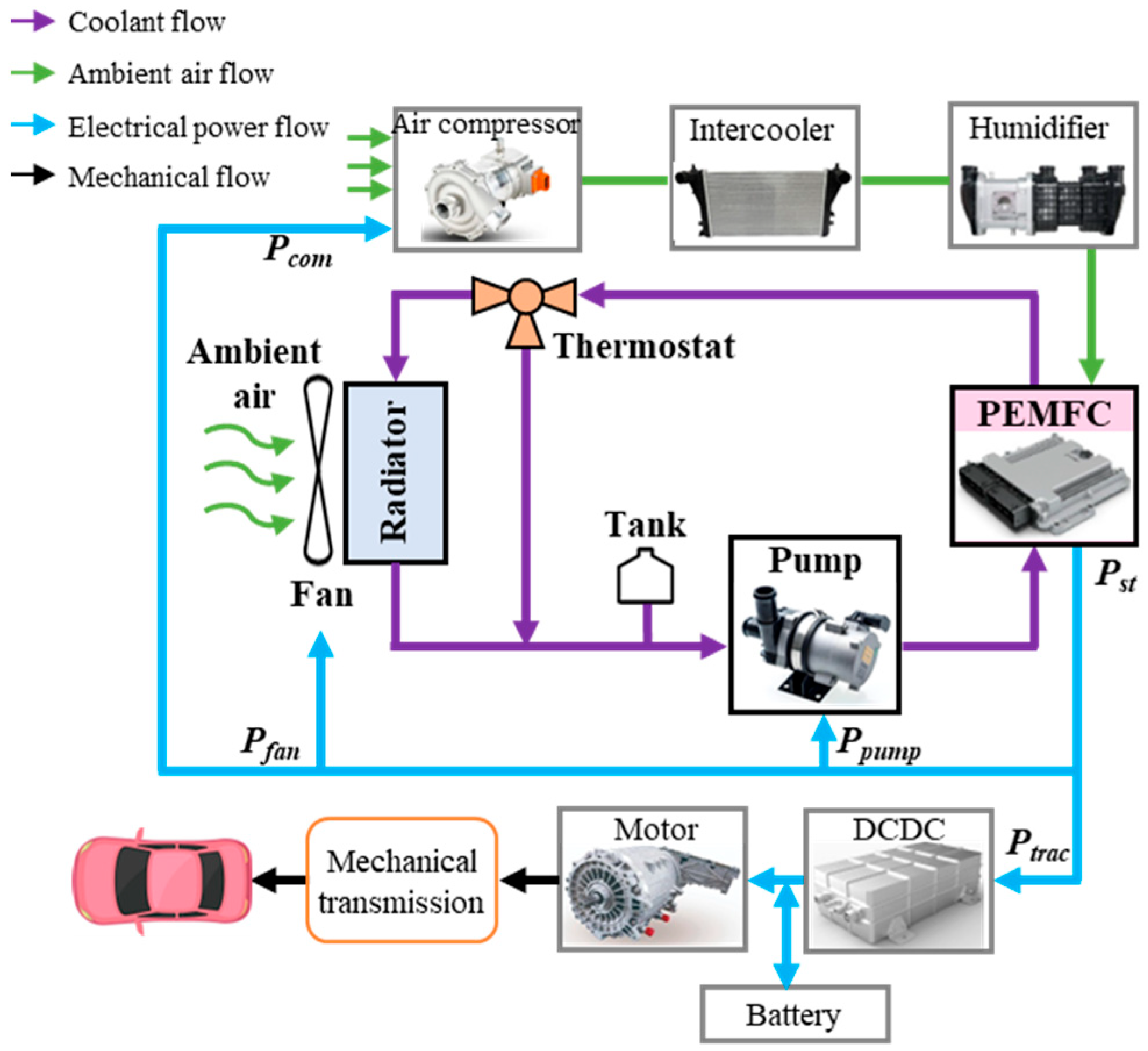
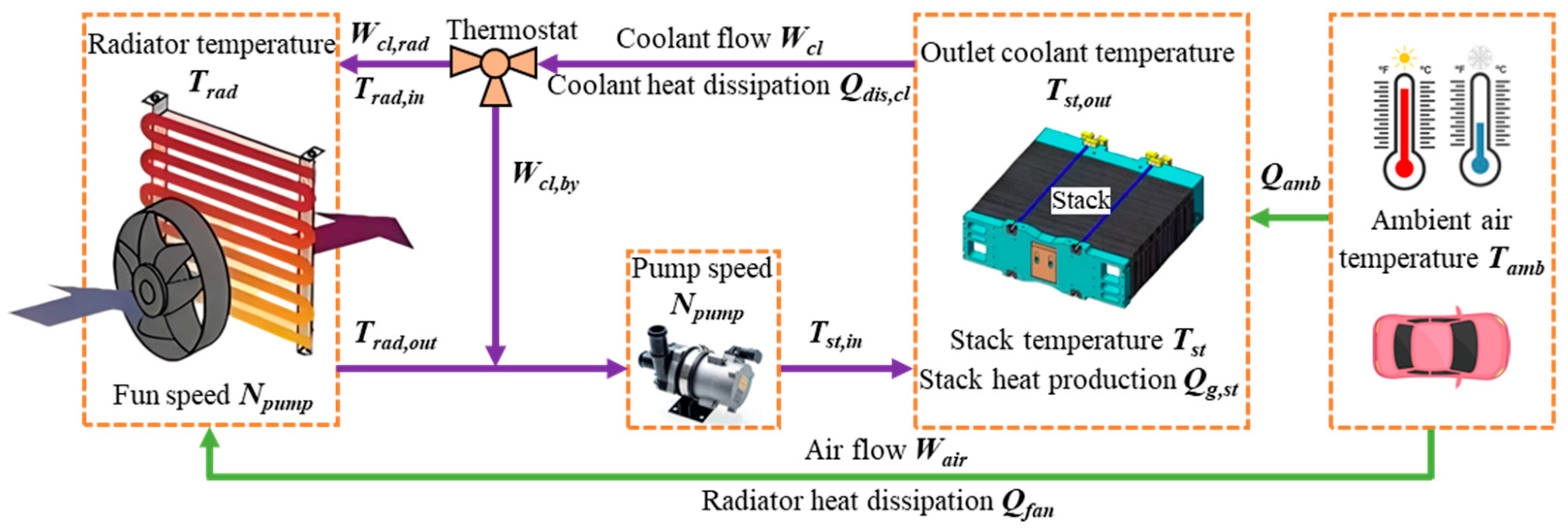
2.1. PEMFC Thermal Management System

The TMS for PEMFC comprises key components including a radiator fan assembly, coolant pump, thermostat, and circulating coolant pipeline. The system’s working principle and energy flow are illustrated in Figure 1. Within designated temperature ranges, the thermostat automatically regulates coolant flow between radiator and bypass circuits, enabling rapid stack warm-up during the startup phase while reducing TMS parasitic losses. As primary actuators, the coolant pump governs stack inlet–outlet coolant temperature gradients to facilitate heat removal, while the radiator regulates inlet coolant temperature via forced-air convection enhanced by the radiator fan. The TMS exhibits inherent nonlinear dynamics characterized by thermal inertia, transport delays, and mutually coupled pump-fan dynamics. Consequently, under stack load transients, significant temperature fluctuations may induce localized overheating and prolonged settling times, potentially compromising operational stability and accelerating PEMFC degradation. Therefore, implementing advanced TMS control strategies—particularly during dynamic load operations—is critical for maintaining thermal stability, ensuring adequate safety margins, and extending system durability.

2.2. PEMFC Thermal Management System Modeling

This study assumes that the temperature distributions within the stack, radiator, and coolant are uniform. Both the stack and the radiator are treated as lumped parameter models. The process of parameter transfer is illustrated in Figure 2.

2.2.1. PEMFC Thermoelectric Coupling Model

According to the heat equilibrium equation $Q=CM\mathrm{\Delta }T$, the thermal balance equation of the stack is expressed as follows:

$$C_{st}{M}_{st}{\displaystyle \frac{d{T}_{st}}{dt}}=Q_{gen,st}-Q_{dis}$$

(1)

where $C_{st}$ is the specific heat capacity of the stack, J/(kg K); $M_{st}$ is the quality of the stack, kg; $T_{st}$ is the stack temperature, K; $Q_{gen,st}$ is the heat generation power of the stack within a unit of time, W; $Q_{dis}$ is the heat dissipation power of the stack within a unit of time, W.

Assuming that all of the chemical energy within the PEMFC is converted, with only electrical energy and thermal energy being produced, the following formula can be used to calculate the heat generation power of the PEMFC.

$$Q_{gen,st}=Q_{theo}-Q_{elec}$$

(2)

where $Q_{theo}$ is the electrochemical energy generated by the stack, W; $Q_{elec}$ is the stack generates electrical energy through electrochemical reactions, W.

$$Q_{theo}=N_{cell}{U}_{nernst}{I}_{st}$$

(3)

The output power of the stack is calculated as the product of the stack voltage and the stack current.

$$Q_{elec}=U_{st}{I}_{st}=N_{cell}{U}_{cell}{I}_{st}$$

(4)

The actual output voltage of a fuel cell is the Nernst open-circuit voltage minus the combined effects of activation polarization loss, ohmic polarization loss, and concentration polarization loss. The actual output voltage of a fuel cell can be expressed as follows:

$$U_{cell}=U_{nernst}-U_{act}-U_{ohmic}-U_{con}$$

(5)

where $U_{nernst}$ is the Nernst open-circuit voltage, V; $U_{act}$ is the activation polarization voltage, V; $U_{ohmic}$ is the ohmic polarization voltage, V; $U_{con}$ is the concentration polarization voltage, V.

Equation (2) can be expressed in the following form.

$$Q_{gen,st}=N_{cell}(U_{nernst}-U_{cell})I_{st}=(N_{cell}{U}_{nernst}-U_{st})I_{st}$$

(6)

Suppose that the hydrogen gas not involved in the electrochemical reaction has no influence on the thermodynamic behavior of the system. The heat transfer analysis of the PEMFC system accounts only for the thermal dissipation associated with the exhaust gas, the produced water, and the coolant. The rate of heat dissipation from the stack per unit time is therefore expressed as follows.

$$Q_{dis}=Q_{sens}+Q_{dis,cl}+Q_{dis,amb}$$

(7)

where $Q_{sens}$ is the amount of heat dissipated by the gas and the produced water, W; $Q_{dis,cl}$ is the stack to coolant heat transfer rate, W; $Q_{dis,amb}$ is the stack to the surrounding environment heat transfer rate, W.

$$Q_{sens}=q_{sens}+q_{cool}+q_{rad}$$

(8)

where $q_{sens}$ is the amount of heat dissipated by gas and produced water per unit time, W. According to the calculations of Yu et al. [43], the total heat dissipation from the gas and generated water can be expressed as the sum of the heat dissipation power associated with the anode gas and water, and that associated with the cathode gas and water,

$$q_{sens}=q_{sens,an}+q_{sens,ca}$$

(9)

where $q_{sens,an}$ and $q_{sens,ca}$, respectively, represent the heat dissipation powers of gases and water at the anode and cathode per unit time, respectively, as expressed by Equations (10) and (11).

$$\begin{array}{c}{q}_{sens,an}=(W_{H_{2,an,out}}{C}_{p,H_2,g}+W_{w,an,g,out}{C}_{p,H_{2}O,g}+W_{w,an,L,out}{C}_{p,H_{2}O,L})\times (T_{an,out}-T_{atm})-\\ (W_{H_{2,an,in}}{C}_{p,H_2,g}+W_{w,an,g,in}{C}_{p,H_{2}O,g}+W_{w,an,L,in}{C}_{p,H_{2}O,L})\times (T_{an,in}-T_{atm})\end{array}$$

(10)

$$\begin{array}{c}{q}_{sens,ca}=(W_{O_{2,ca,out}}{C}_{p,O_2,g}+W_{N_2,ca,out}{C}_{p,N_2,g}+W_{w,ca,g,out}{C}_{p,H_{2}O,g}+W_{w,ca,L,out}{C}_{p,H_{2}O,L})\times (T_{ca,out}-T_{atm})-\\ (W_{O_{2,ca,in}}{C}_{p,O_2,g}+W_{N_2,ca,in}{C}_{p,N_2,g}+W_{w,ca,g,in}{C}_{p,H_{2}O,g}+W_{w,ca,L,in}{C}_{p,H_{2}O,L})\times (T_{ca,in}-T_{atm})\end{array}$$

(11)

According to the heat balance equation, the heat dissipated by the coolant circulating through the stack is as follows:

$$Q_{dis,cl}=W_{cl}{C}_{p,cl}(T_{st}-T_{st,in})$$

(12)

where $W_{cl}$ is the coolant flow rate, kg/s; $C_{p,cl}$ is the coolant specific heat capacity, kJ/(kg K); $T_{st,in}$ is the stack inlet coolant temperature, K.

The heat emitted by the stack into the environment is as follows:

$$Q_{dis,amb}=(T_{st}-T_{amb})/R_t$$

(13)

where $T_{amb}$ is the ambient temperature, K; $R_t$ is the thermal resistance of heat transfer between the stack and the environment, K/W.

Based on the electron transfer process during the generation of electrical energy through hydrogen–oxygen chemical reactions, mathematical expressions for the output current and $H_2$ consumption rate of the PEMFC are derived.

$$n_{H_2}={\displaystyle \frac{I_{st}\cdot N_{cell}}{2F}}$$

(14)

where $n_{H_2}$ is the number of moles of $H_2$ participating in the reaction and generating electric current, mol; $F$ is the Faraday constant, 96,500 C/mol.

The above formula can be converted to represent the mass flow rate of $H_2$ consumption, which is expressed as follows:

$$m_{fc}={\displaystyle \frac{m_{H_2}\cdot 60\cdot I_{st}\cdot N_{cell}}{2\cdot {\phi }_{H_2}\cdot F\cdot {\rho }_{H_2}}}$$

(15)

where $m_{H_2}$ is the molar mass of $H_2$, g/mol; ${\phi }_{H_2}$ is the mass fraction of $H_2$.

2.2.2. Radiator Heat Transfer Model

The temperature of the coolant at the radiator inlet, the temperature of the coolant at the stack outlet, and the stack temperature are considered to be equal.

$$T_{rad,in}=T_{st,out}=T_{st}$$

(16)

where $T_{rad,in}$ is the coolant temperature at the inlet of the radiator, K; $T_{st,out}$ is the coolant temperature at the outlet of the stack, K.

The radiator temperature $T_{rad}$ is defined as the average of the coolant temperatures measured at the radiator’s inlet and outlet.

$$T_{rad}=(T_{st}+T_{st,out})/2$$

(17)

The heat balance equation for the radiator can be expressed as follows:

$${\rho }_{rad}{V}_{rad}{C}_{p,rad}{\displaystyle \frac{d{T}_{rad}}{dt}}=Q_{cl,rad}-Q_{fan}$$

(18)

where ${\rho }_{rad}$ is the radiator average density, kg/m³; $V_{rad}$ is the volume of the radiator coolant flow channel, m³; $C_{p,rad}$ is the average specific heat capacity of the radiator, kJ/(kg·K); $Q_{cl,rad}$ is the heat dissipation capacity of the coolant in the radiator, W; $Q_{fan}$ is the heat dissipation capacity of the radiator fan, W.

The radiator fan facilitates the exchange of heat between the coolant in the circuit and the external environment. The heat dissipation capacity of the radiator fan is as follows:

$$Q_{fan}=W_{air}{C}_{p,air}\left[(T_{st}+T_{rad,out})/2-T_{atm}\right]$$

(19)

where $W_{air}$ is the flow rate of the air passing through the fan, kg/s; $C_{p,air}$ is the heat capacity of air at constant pressure, kJ/(kg·K).

The cooling capacity of the radiator is as follows:

$$Q_{cl,rad}=W_{cl}{C}_{p,cl}(T_{st}-T_{rad,out})$$

(20)

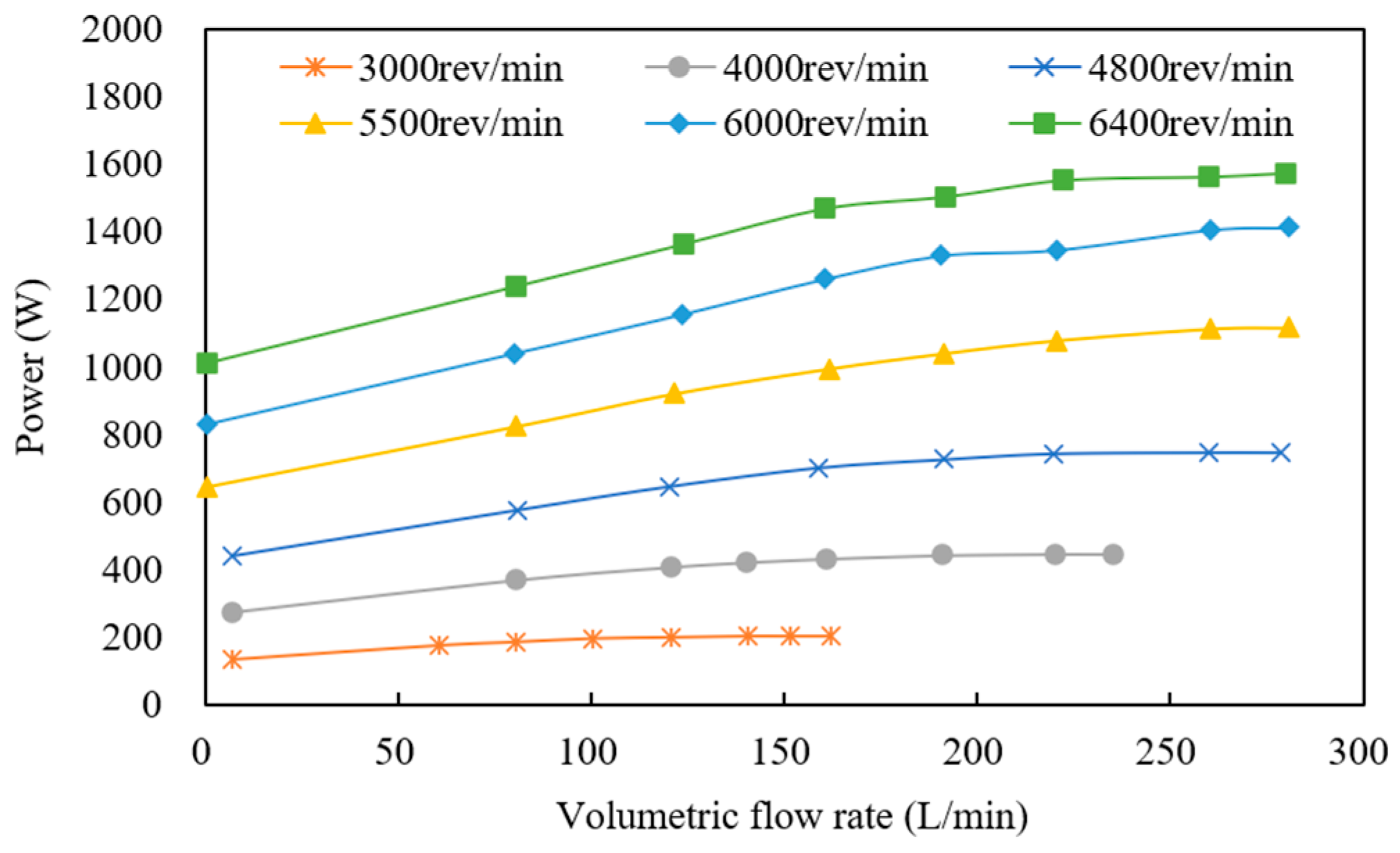
2.2.3. Pump and Fan Model

According to the principle of affinity laws, the relationship between the speed and the flow rate of the pump can be determined.

$${\displaystyle \frac{W_{cl,2}}{N_{pump,2}}}={\displaystyle \frac{W_{cl,1}}{N_{pump,1}}}$$

(21)

where $W_{cl,2}$ is the coolant flow rate corresponding to the speed $N_{pump,2}$ of the pump, kg/s; $W_{cl,1}$ is the flow rate corresponding to the speed $N_{pump,1}$, kg/s; $N_{pump,1}$ and $N_{pump,2}$ are the pump speed, rev/min.

The actual power output of the pump is determined by the indicated power and the corresponding efficiency.

$$P_{pump,in}=P_{pump}{\eta }_{pump}={\rho }_{cl}g{H}_{pump}{V}_{pump}{N}_{pump}/60$$

(22)

where $P_{pump,in}$ is the pump indicated power, W; $P_{pump}$ is the actual power, W; ${\eta }_{pump}$ is the efficiency of the pump, %; $H_{pump}$ is the head of the pump, m, which is determined by the system pressure; $V_{pump}$ is the pumping capacity of the pump, m³.

Figure 3 depicts the pump power–coolant flow rate relationship derived from characteristic experiments. The data demonstrate that lower pump speeds reduce power consumption at equivalent flow rates, albeit with constrained operable flow ranges. Consequently, minimizing speed fluctuations is essential to maintain operation within peak efficiency zones. The operational speed range must be dynamically adjusted according to thermal load requirements, which dictate permissible speed variation limits. During high-power demand scenarios, the allowable speed range proportionally expands.

Fan power calculation follows principles analogous to pump systems. Per affinity laws, airflow rate exhibits proportional dependence on rotational speed, while power demonstrates cubic dependence. Consequently, minimizing fan energy consumption requires maintaining rotational speed at the minimum sustainable level.

$$W_{fan,2}=W_{fan,1}\cdot {\displaystyle \frac{N_{fan,2}}{N_{fan,1}}}$$

(23)

$$P_{fan,2}=P_{fan,1}\cdot {\left({\displaystyle \frac{N_{fan,2}}{N_{fan,1}}}\right)}^3$$

(24)

where $W_{fan,1}$ and $W_{fan,2}$ are the respective air flow rates corresponding to fan speeds $N_{fan,1}$ and $N_{fan,2}$, kg/s; $P_{fan,1}$ and $P_{fan,2}$ are the power consumption of the fan at speeds $N_{fan,1}$ and $N_{fan,2}$, respectively, W.

This study selects the energy consumption ($E_{total}$) of the pump and fan as the key energy consumption evaluation indicator for the TMS.

$$E_{total}=P_{total}\cdot t$$

(25)

$$P_{total}=P_{pump}+P_{fan}$$

(26)

where $E_{total}$ is the total energy consumption of the pump and the fan, J; $P_{total}$ is the sum of the power of the pump and the fan, W; $t$ is the operating time of the pump and the fan, s.

2.2.4. Thermostat Model

The TMS of PEMFC comprises two coolant circuits: radiator and bypass paths. A three-way thermostat modulates coolant flow distribution between these paths based on stack outlet coolant temperature. When stack temperature falls below a set threshold, the thermostat closes the radiator path to accelerate warm-up. Conversely, when exceeding a defined threshold, the thermostat proportionally opens the radiator path while maintaining full bypass flow. Valve position is quantitatively expressed as follows:

$$W_{cl}{T}_{tv,out}={\kappa }_{tv}{W}_{cl}{T}_{rad,out}+(1-{\kappa }_{tv})W_{cl}{T}_{st,out}$$

(27)

where $T_{tv,out}$ is the temperature of the coolant as it exits the thermostat outlet, K; ${\kappa }_{tv}$ is the degree of valve opening, and the range is 0 ≤ ${\kappa }_{tv}$ ≤ 1.

3. PEMFC Model Validation

This section presents the relevant experimental data obtained through the established PEMFC experimental platform, aimed at validating the constructed PEMFC model and determining the relationship between the PEMFC’s output power and its OOT.

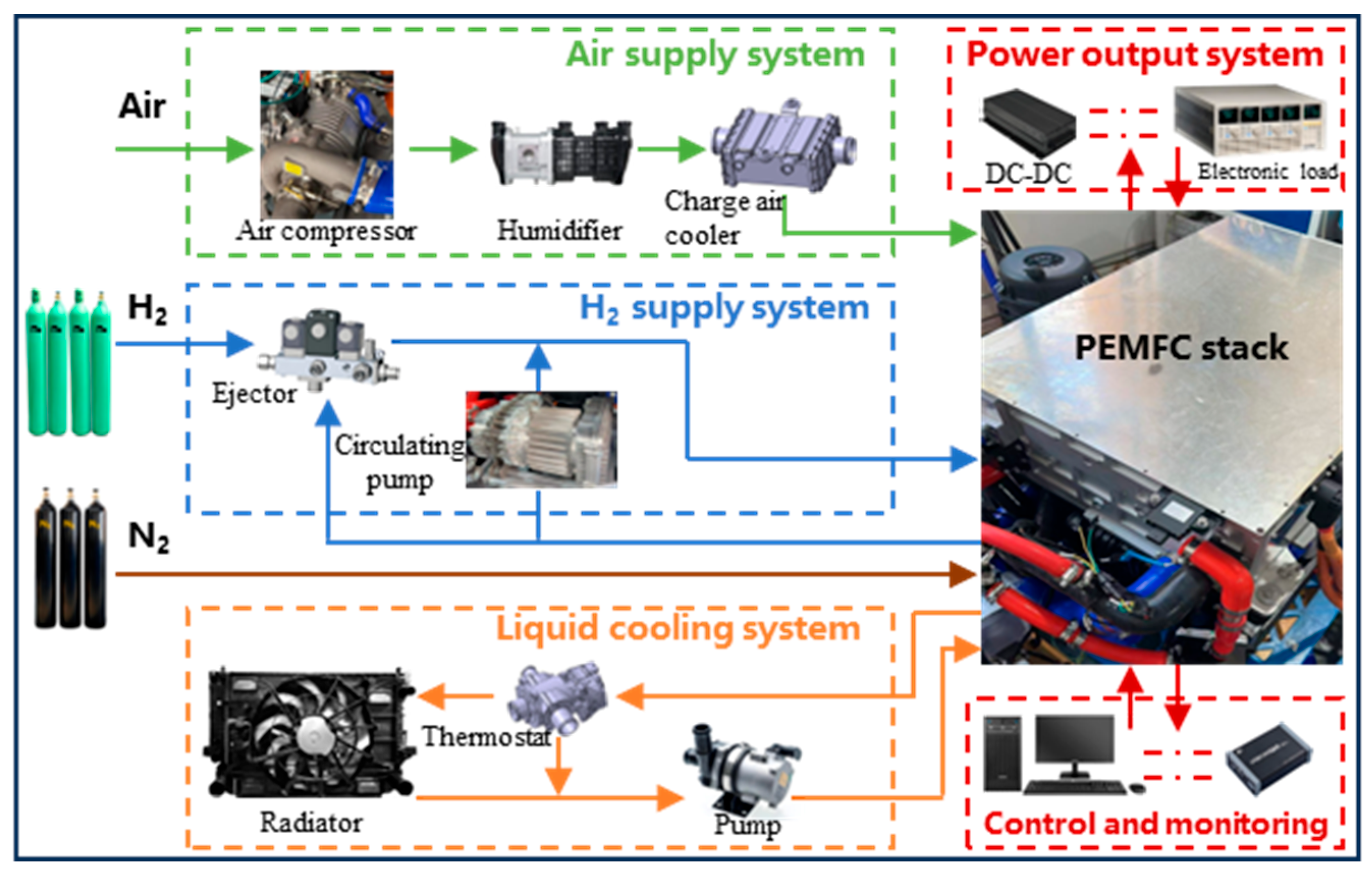
3.1. PEMFC Experimental Platform

To ensure stable power output under variable operating conditions, the PEMFC system integrates five critical subsystems: (1) a gas supply subsystem (air/H₂/N₂) for reactive gas delivery and purge protection; (2) a liquid-cooled thermal management subsystem maintaining stack thermal equilibrium; (3) a power management and monitoring subsystem enabling power delivery and protection; (4) a control and data acquisition subsystem handling signal transmission and coordination; and (5) an auxiliary and safety subsystem managing exhaust treatment and safety safeguards. These subsystems, integrated with supervisory control and data acquisition software, constitute the complete experimental PEMFC system (Figure 4). Key stack and TMS component specifications are summarized in

Table 1. Summary of relevant PEMFC system components specifications.

Component	Description	Specification
Fuel cell stack	Maximum output power	87 kW
	Cells	290
	Cells active area	282 cm2
	Oxidant composition	0.21
Radiator	Frontal area	0.38 m2
	Maximum heat dissipation	120 kW
Radiator fan	Diameter dimension	384 mm
Temperature sensor	Type	Type T thermocouple
	Precision	±0.5 °C

. This experimental platform facilitated comprehensive stack characterization studies.

3.2. Model Validation

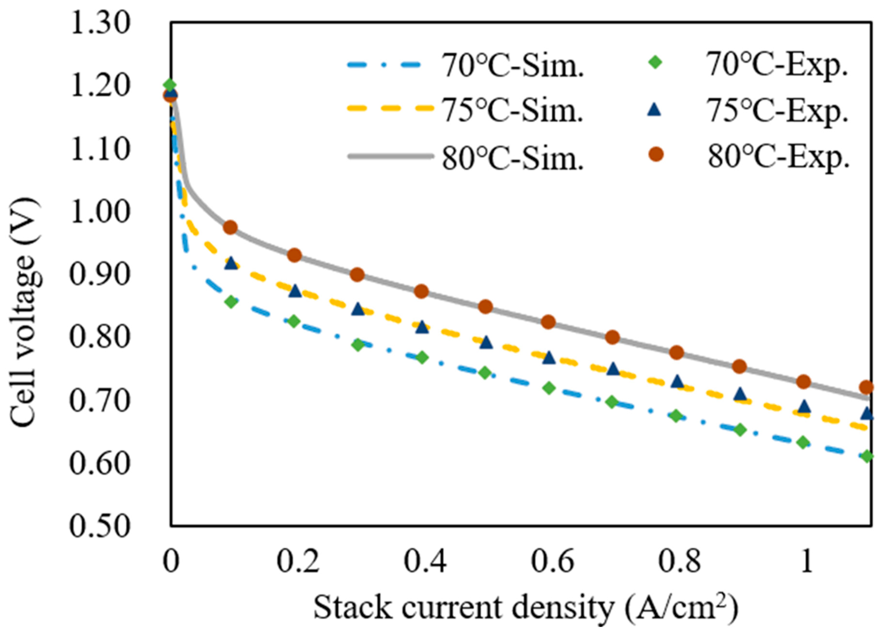
3.2.1. PEMFC Voltage Model

Experimental I-V curves of the stack operating at 70 °C, 75 °C, and 80 °C were obtained under conditions specified in

Table 2. Experiment conditions.

Parameter	Value
Cathode air inlet pressure	155 kPa
Cathode hydrogen inlet pressure	150 kPa
Ambient temperature	20 °C
Stack operating temperature	70 °C/75 °C/80 °C
Electric current density	0/0.1/0.2/0.3/0.4/0.5/0.6/0.7/0.8/0.9/1.0/1.1 A/cm2

. The current density range spanned 0–1.1 A/cm². Transient voltage oscillations occurred during load current transitions prior to steady-state stabilization. Consequently, current and voltage values were recorded via the host computer monitoring system after operational stability was achieved, with the stack output voltage averaged at each current density point. The stack I-V curves are presented in Figure 2. Comparative experimental and simulation results across temperatures are shown in Figure 5, with corresponding errors quantified in

Table 3. Errors of experimental results and simulation results at various operating temperatures.

Operating Temperature	MAE	MaxAE
70 °C	0.0024 V	0.0103 V
75 °C	0.0032 V	0.0135 V
80 °C	0.0026 V	0.0117 V

. The mean absolute error (MAE) remained below 0.0032 V, while the maximum absolute error (MaxAE) did not exceed 0.0135 V. These results demonstrate that the established model has high accuracy. Error sources include disparities between assumed material properties and actual components, inherent system uncertainties, and deliberate model simplifications.

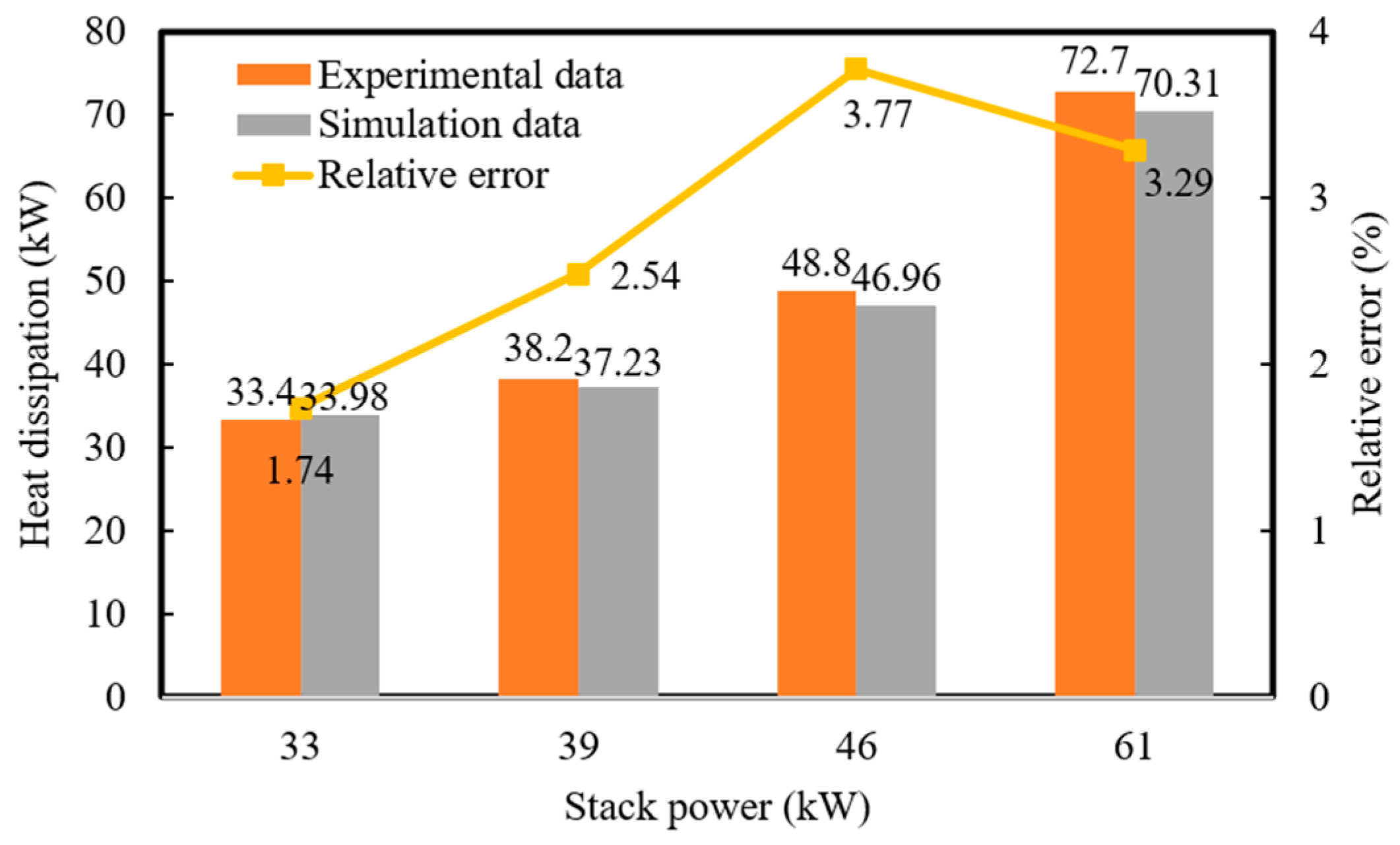
3.2.2. PEMFC Heat Generation Model

To validate the adaptability of the developed PEMFC heat generation model under different operating conditions, steady-state stack thermal dissipation calculations were compared with experimental measurements, as presented in Figure 6. Despite minor deviations attributable to model simplifications and experimental uncertainties, the maximum error remained below 3.77%, demonstrating model reliability.

3.3. Experiment on the OOT of PEMFC

Experimental investigation of the relationship between output power and optimal operation for the fuel cell system employed in this study was conducted under the following conditions: The temperature varied from 50 °C to 90 °C in 4 °C increments, with current ranging from 60 to 410 A. The experimental protocol included the following: (1) provision of stable power to the electric water pump, air compressor, hydrogen recirculation pump, and host monitoring platform via a high-voltage power supply; (2) implementation of constant-current output mode through command signals transmitted from the host computer to the fuel cell control system via the CAN bus communication protocol; (3) precise thermal management through real-time regulation of coolant pump speed and radiator fan velocity by preset parameters in the host control interface; (4) synchronous recording of stack temperature and output voltage dynamics at a 1 Hz sampling frequency using integrated temperature sensing and voltage acquisition modules. Optimal temperature operating points were determined at each current level, enabling derivation of the system’s efficiency-optimized operational trajectory.

Figure 7a reveals that at a constant stack current, output power initially rises then declines with increasing operating temperature, indicating the existence of an optimal operating temperature (OOT) for maximum power output. Per Equation (15), hydrogen consumption remains constant under fixed current. Consequently, PEMFC efficiency peaks at the maximum power output, establishing this temperature as the OOT. Deviations from OOT (either above or below) require increased current to deliver specified power, elevating hydrogen consumption. Therefore, maintaining stack temperature at optimal levels is essential. The OOT curve (Figure 7b), constructed by mapping peak power temperatures at each constant current, provides the reference trajectory for MPC control.

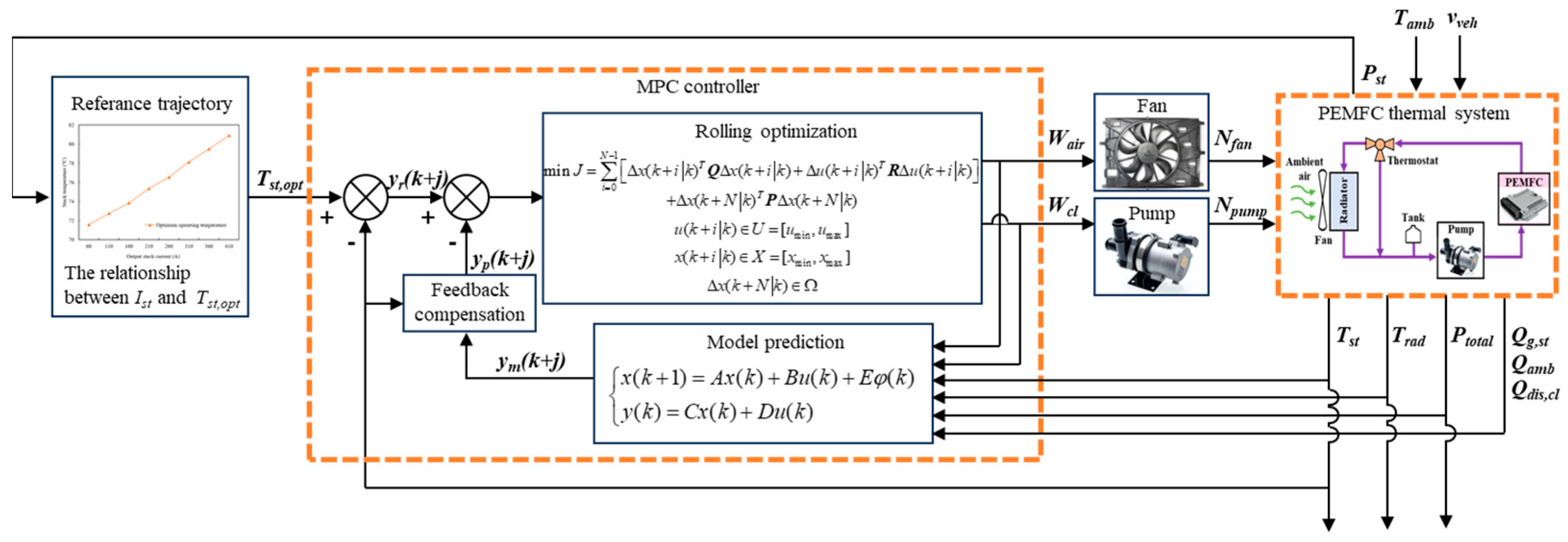
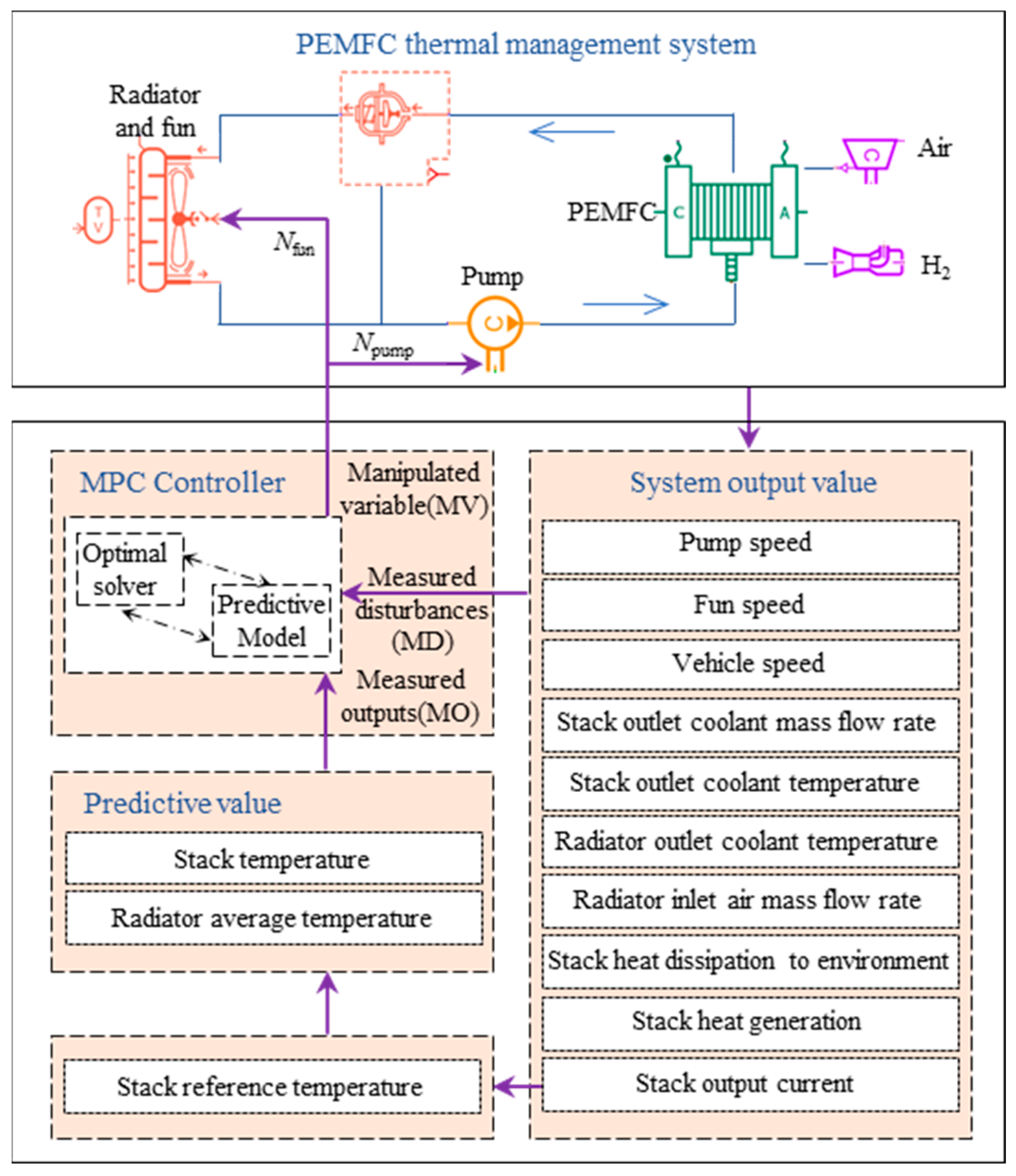
4. PEMFC Thermal Management MPC Controller Design

This section designs an MPC strategy for OOT tracking, targeting minimization of both operating temperature deviation from OOT and parasitic power consumption in PEMFC. The TMS model is linearized and discretized to establish a real-time switchable predictive model applicable to PEMFC under variable load conditions. Validation employs the Worldwide Harmonized Light Vehicles Test Cycle (WLTC).

4.1. MPC Controller Design

The controller is designed based on the MPC method to regulate the speeds of the radiator fan $N_{fan}$ and the coolant pump $N_{pump}$ within the PEMFC’s TMS, thereby enabling control over the operating temperature of the PEMFC. Using the stack output power as the input parameter, the OOT of the stack at this output power is derived from the output power–OOT curve. Both the OOT and the current actual operating temperature of the stack are then input to the MPC controller. Through model-based prediction and rolling optimization, the controller calculates the optimal control outputs—specifically, the desired speeds $N_{fan}$ and $N_{pump}$. The schematic diagram of the control process is shown in Figure 8.

The controller dynamically adjusts $N_{fan}$ and $N_{pump}$ in real-time based on stack thermal load and the vehicular operating conditions, selecting optimal combinations that satisfy the coolant temperature requirements while minimizing energy consumption. The primary control objectives are $T_{st}$ and $P_{total}$, though these exhibit significant magnitude disparities. The direct optimization of $P_{total}$ may destabilize $T_{st}$ control. Figure 3 demonstrates that reduced speed decreases pump power consumption at equivalent flow rates, albeit with constrained operable flow ranges. Consequently, speed interval partitioning according to thermal load requirements enables indirect subsystem energy optimization. The proposed controller architecture integrates model prediction and rolling optimization components, implemented as follows.

4.1.1. Model Prediction

Effective MPC implementation requires designing a predictive model to forecast future system states. Linear MPC is employed to conserve computational resources and ensure closed-loop stability. The linearized model may be derived either through system identification or by linearizing the dynamic model at equilibrium points. Building upon the nonlinear thermal dynamics model established in Section 2, we develop a state-space internal model expressed as follows:

$$\left\{\begin{array}{l}\dot{\mathit{x}}=\mathit{A}\mathit{x}+\mathit{B}\mathit{u}+\mathit{E}\mathit{\phi }\\ \mathit{y}=\mathit{C}\mathit{x}+\mathit{D}\mathit{u}\end{array}\right.$$

(28)

where $\mathit{x}$ is the state vector, $\mathit{x}={\left[\begin{array}{cc}{T}_{st}& T_{rad}\end{array}\right]}^T$; $\mathit{u}$ is the input vector, $\mathit{u}={\left[\begin{array}{cc}{W}_{cl}& W_{air}\end{array}\right]}^T$; $\mathit{\phi }$ is the disturbance vector, $\mathit{\phi }={\left[\begin{array}{cc}{Q}_{g,st}& Q_{amb}\end{array}\right]}^T$. The output temperature $T_{st}$ can be monitored via the temperature sensor installed at the outlet of the stack; therefore, it is selected as the output variable for the controller, represented by $\mathit{y}=\left[T_{st}\right]$. $\mathit{A}$ is the system matrix; $\mathit{B}$ is the input matrix; $\mathit{C}$ is the output matrix; $\mathit{D}$ is the feedthrough matrix; $\mathit{E}$ is the disturbance matrix.

Most of the heat generated by the PEMFC is dissipated via the coolant. In this study, the heat transfer between the coolant in the piping system and the external environment is neglected. It is assumed that all the thermal energy in the coolant is dissipated through the radiator. The coolant temperature at the stack outlet is approximately equal to that at the radiator inlet, while the coolant temperature at the stack inlet is approximately equal to that at the radiator outlet. Consequently, the operating temperature of the PEMFC can be expressed as follows:

$${\displaystyle \frac{d{T}_{st}}{dt}}={\displaystyle \frac{Q_{g,st}-Q_{dis,cl}-Q_{dis,amb}}{C_{p,st}{M}_{st}}}$$

(29)

By substituting Equation (13) into the above equation, the following result is obtained:

$${\displaystyle \frac{d{T}_{st}}{dt}}={\displaystyle \frac{Q_{g,st}-Q_{dis,amb}-C_{cl}\cdot W_{cl}(T_{st}-T_{st,in})}{C_{p,st}{M}_{st}}}$$

(30)

The radiator enables forced heat dissipation from the coolant to the ambient air via fan operation. The heat balance equation for the radiator is as follows:

$${\displaystyle \frac{d{T}_{rad}}{dt}}={\displaystyle \frac{Q_{dis,cl}-Q_{fan}}{C_{p,rad}{M}_{rad}}}$$

(31)

The heat dissipation capacity of the radiator fan is as follows:

$$Q_{fan}=W_{air}{C}_{p,air}\left[(T_{st}+T_{rad,out})/2-T_{amb}\right]$$

(32)

The heat dissipation capacity of the coolant is as follows:

$$Q_{dis,cl}=W_{cl}{C}_{p,cl}(T_{rad,in}-T_{rad,out})$$

(33)

The temperature of the radiator is defined as the average of the coolant temperatures measured at its inlet and outlet.

$$T_{rad}=(T_{st}+T_{rad,out})/2$$

(34)

The coolant temperature at the radiator inlet and the coolant temperature at the stack outlet are identical to the stack temperature, namely,

$$T_{rad,in}=T_{st,out}=T_{st}$$

(35)

In the MPC approach, the Taylor series expansion is employed to linearize the system around a specific operating point, yielding the following linearized model:

$$\left\{\begin{array}{l}\dot{\tilde{\mathit{x}}}=\mathit{A}\tilde{\mathit{x}}+\mathit{B}\tilde{\mathit{u}}+\mathit{E}\tilde{\mathit{\phi }}\\ \tilde{\mathit{y}}=\mathit{C}\tilde{\mathit{x}}+\mathit{D}\tilde{\mathit{u}}\end{array}\right., \tilde{\mathit{x}}=\mathit{x}-{\mathit{x}}_{\mathit{o}\mathit{p}},\tilde{\mathit{u}}=\mathit{u}-{\mathit{u}}_{\mathit{o}\mathit{p}},\tilde{\mathit{y}}=\mathit{y}-{\mathit{y}}_{\mathit{o}\mathit{p}}$$

(36)

where, $\mathit{A}=\left(\begin{array}{cc}1-{\displaystyle \frac{2C_{p,cl}{N}_{pump(op)}}{C_{p,st}{M}_{st}}}\hfill & 0\\ {\displaystyle \frac{2C_{cl}(T_{rad(op)}-T_{st(op)})}{C_{p,st}{M}_{st}}}\hfill & 1-{\displaystyle \frac{2C_{cl}{N}_{pump(op)}-C_{p,air}{N}_{fan(op)}}{C_{p,rad}{M}_{rad}}}\hfill \end{array}\right)$,

$\mathit{B}=\left(\begin{array}{cc}{\displaystyle \frac{2C_{cl}(T_{rad(op)}-T_{st(op)})}{C_{p,st}{M}_{st}}}\hfill & 0\\ ({\displaystyle \frac{2C_{cl}(T_{st(op)}+T_{rad(op)})}{C_{p,rad}{M}_{rad}}})\hfill & {\displaystyle \frac{C_{p,air}(T_{amb}-T_{rad(op)})}{C_{p,rad}{M}_{rad}}}\hfill \end{array}\right)$,

$\mathit{E}=\left(\begin{array}{cc}{\displaystyle \frac{1}{C_{p,st}{M}_{st}}}\hfill & {\displaystyle \frac{2C_{cl}}{C_{p,st}{M}_{st}}}(T_{st(op)}{W}_{cl(op)}-T_{rad(op)}{W}_{cl(op)})\\ 0& {\displaystyle \frac{T_{rad(op)}(C_{p,air}{W}_{air(op)}-2C_{cl}{W}_{cl(op)})}{C_{p,rad}{M}_{rad}}}\end{array}\right)$, $\mathit{C}=\left[\begin{array}{cc}1& 1\end{array}\right]$, $\mathit{D}=\left[\begin{array}{cc}0& 0\end{array}\right]$.

The state-space model is discretized via the forward Euler method, where $t_s$ denotes the sampling period. The predictive model can be expressed as follows:

$$\left\{\begin{array}{l}\tilde{\mathit{x}}(k+1)={\mathit{A}}_k\tilde{\mathit{x}}(k)+{\mathit{B}}_k\tilde{\mathit{u}}(k)+\mathit{E}\tilde{\mathit{\phi }}(k)\\ \tilde{\mathit{y}}(k)={\mathit{C}}_k\tilde{\mathit{x}}(k)+{\mathit{D}}_k\tilde{\mathit{u}}(k)\end{array}\right.$$

(37)

where k is the control step, k + 1 is the subsequent step; $\mathit{x}(k)$ is the state of the system at time k; $\mathit{u}(k)$ is the control input of the system at the k-th step; $\mathit{\phi }(k)$ is the disturbance variable of the system at step k. ${\mathit{A}}_k=\mathit{I}+t_s\mathit{A}$, ${\mathit{B}}_k=t_s\mathit{B}$.

Owing to the nonlinear characteristics of the PEMFC’s TMS, the predictive accuracy of linear models deteriorates as operating conditions deviate from the nominal point. To mitigate this limitation, distinct predictive models were developed for varying load conditions, with real-time switching enabled upon changes in operational conditions. In this study, three linear models corresponding to distinct operating points were selected to effectively characterize the typical load conditions of the TMS. For the 87 kW automotive PEMFC system, output currents of 60 A, 200 A, and 300 A were chosen as representative operating points. These values correspond to low-, medium-, and high-load conditions of the PEMFC system, respectively, and are integrated into the design of a multi-model switching MPC strategy. When the output current is below 120 A, it is classified as a low-power operating condition, with the operating point corresponding to 60 A, and the control strategy prioritizing energy efficiency. When the current range is between 120 and 240 A, it is categorized as a medium-power operating condition, with the operating point corresponding to 200 A, and the control strategy aiming to balance the response speed and thermal management efficiency. When the current range is between 240 and 410 A, it is classified as a high-power operating condition, with the operating point corresponding to 240 A, and the primary objective of the control strategy is to maximize heat dissipation capacity. The switching logic of the predictive models is structured as follows.

$$\left[\begin{array}{cc}{\mathit{A}}_k& {\mathit{B}}_k\\ {\mathit{C}}_k& {\mathit{D}}_k\end{array}\right]=\left\{\begin{array}{c}\left[\begin{array}{cc}{\mathit{A}}_1& {\mathit{B}}_1\\ {\mathit{C}}_1& {\mathit{D}}_1\end{array}\right],I_{st}\in \left[0,120\right]\\ \left[\begin{array}{cc}{\mathit{A}}_2& {\mathit{B}}_2\\ {\mathit{C}}_2& {\mathit{D}}_2\end{array}\right],I_{st}\in \left[120,240\right]\\ \left[\begin{array}{cc}{\mathit{A}}_3& {\mathit{B}}_3\\ {\mathit{C}}_3& {\mathit{D}}_3\end{array}\right],I_{st}\in \left[240,410\right]\end{array}\right.$$

(38)

To improve prediction accuracy, the current actual system state is used as the initial condition for each control step. For this system, the state error can be formulated as follows:

$$e(k)=\widehat{x}(k)-\widehat{x}(k|k-1)$$

(39)

where $\widehat{x}(k|k-1)$ is the predicted system output state at time k, derived from the state estimation at time k − 1.

The estimated state for the subsequent time step can be expressed as follows:

$$\widehat{x}(k+1|k)=A_k\widehat{x}(k|k-1)+B_k\widehat{u}(k|k-1)+E\widehat{\phi }(k|k-1)$$

(40)

The system’s predicted output over the next Np steps can be represented as follows:

$$Y_p(k)=S_x\widehat{X}(k)+S_{\mathrm{\Delta }u}\mathrm{\Delta }U(k)+S_{\phi }\mathsf{\Phi }(k)$$

(41)

where, $Y_p=\left[\begin{array}{c}\begin{array}{c}\begin{array}{c}y(k+1\left|k\right.)\\ y(k+2\left|k\right.)\end{array}\\ \cdot \cdot \cdot \end{array}\\ y(k+N_c\left|k\right.)\\ \cdot \cdot \cdot \\ y(k+N_p\left|k\right.)\end{array}\right]$, $S_x=\left[\begin{array}{c}\begin{array}{c}\begin{array}{c}{C}_k{A}_k\\ C_k{A_k}^2\end{array}\\ \cdot \cdot \cdot \end{array}\\ C_k{A_k}^{N_c}\\ \cdot \cdot \cdot \\ C_k{A_k}^{N_p}\end{array}\right]$, $\mathrm{\Delta }U(k)=\left[\begin{array}{c}\mathrm{\Delta }u(k\left|k\right.)\\ \mathrm{\Delta }u(k+1\left|k\right.)\\ \cdot \cdot \cdot \\ \mathrm{\Delta }u(k+N_c-1\left|k\right.)\end{array}\right]$, $S_{\mathrm{\Delta }u}=\left[\begin{array}{cccc}{C}_k{B}_k& 0& 0& \begin{array}{cc}\dots & 0\end{array}\\ C_k{A}_k{B}_k& C_k{B}_k& 0& \begin{array}{cc}\dots & 0\end{array}\\ ⋮& ⋮& ⋮& \begin{array}{cc}\ddots & ⋮\end{array}\\ \begin{array}{c}{C}_k{\displaystyle \sum _{i=0}^{N_c-1}{A_k}^i{B}_k}\\ C_k{\displaystyle \sum _{i=0}^{N_c}{A_k}^i{B}_k}\\ \begin{array}{c}⋮\\ C_k{\displaystyle \sum _{i=0}^{N_p-1}{A_k}^i{B}_k}\end{array}\end{array}& \begin{array}{c}{\displaystyle \sum _{i=0}^{N_c-2}{A_k}^i{B}_k}\\ {\displaystyle \sum _{i=0}^{N_c-1}{A_k}^i{B}_k}\\ \begin{array}{c}⋮\\ {\displaystyle \sum _{i=0}^{N_p-2}{A_k}^i{B}_k}\end{array}\end{array}& \begin{array}{c}\dots \\ \dots \\ \dots \end{array}& \begin{array}{cc}\begin{array}{c}\dots \\ \dots \\ \begin{array}{c}⋮\\ \dots \end{array}\end{array}& \begin{array}{c}{C}_k{B}_k\\ C_k{A}_k{B}_k\\ \begin{array}{c}⋮\\ C_k{\displaystyle \sum _{i=0}^{N_p-N_c}{A_k}^i{B}_k}\end{array}\end{array}\end{array}\end{array}\right]$, $S_{\phi }=\left[\begin{array}{cccc}{C}_k{B}_k& 0& \dots & 0\\ C_k{A}_k{B}_k& C_k{B}_k& \dots & 0\\ ⋮& ⋮& \dots & 0\\ C_k{A_k}^{N_p-1}{B}_k& C_k{A_k}^{N_p-2}{B}_k& \dots & C_k{B}_k\end{array}\right]$, N_p and N_c denote the prediction horizon and the control horizon.

4.1.2. Rolling Optimization

In PEMFC auxiliary system control, actuator limitations and safety constraints necessitate precise reference tracking while maintaining control input variations within acceptable bounds. At each sampling time k, $x(k+i|k)$ and $u(k+i|k)$ denote the predicted state and the predicted input sequence for the $k+i$ time step, respectively. The optimization objective $J$ formulated as shown in Equation (42) incorporates quadratic terms for both tracking error and the control input variation, enabling explicit trade-offs between reference trajectory accuracy and control input smoothness.

$$\begin{array}{c}\min J={\displaystyle \sum _{i=0}^{N-1}\left[\mathrm{\Delta }x{(k+i\left|k\right.)}^T\mathit{Q}\mathrm{\Delta }x(k+i\left|k\right.)+\mathrm{\Delta }u{(k+i\left|k\right.)}^T\mathit{R}\mathrm{\Delta }u(k+i\left|k\right.)\right]}\\ +\mathrm{\Delta }x{(k+N\left|k\right.)}^T\mathit{P}\mathrm{\Delta }x(k+N\left|k\right.)\end{array}$$

(42)

$$\mathit{s}\mathit{\text{.}}\mathit{t}\mathit{\text{.}} x(k+1)=f(x(k),u(k),Q_{g,st}(k),Q_{amb}(k))$$

$$N_{fan,\min }\le N_{fan}(k)\le N_{fan,\max }$$

$$N_{pump,\min }\le N_{pump}(k)\le N_{pump,\max }$$

$$\mathrm{\Delta }{N}_{fan,\min }\le \mathrm{\Delta }{N}_{fan}(k)\le \mathrm{\Delta }{N}_{fan,\max }$$

$$\mathrm{\Delta }{N}_{pump,\min }\le \mathrm{\Delta }{N}_{pump}(k)\le \mathrm{\Delta }{N}_{pump,\max }$$

where $J$ is the cost function. $u$ is the predictive input. $x$ is the predicted state. $\mathrm{\Delta }x$ is the predicted trajectory and the expected error, $\mathrm{\Delta }\widehat{x}=\widehat{x}-r$. $r$ is the expected state. $\mathrm{\Delta }u$ is the deviation between the predicted input and the equilibrium point input, $\mathrm{\Delta }u=u-u_r$. $u_r$ is the anticipated equilibrium point input. $N$ is the predicted state and predicted input horizon. Q is the weight matrix of the predicted state. R is the weight matrix of the predicted input. P is the weight matrix of the terminal cost function.

Meanwhile, the predicted state weight matrix Q and the predicted input weight matrix R are defined as follows:

$$\mathit{Q}\stackrel{def}{=}diag(Q_1,Q_2,\cdot \cdot \cdot ,Q_j)$$

(43)

$$\mathit{R}\stackrel{def}{=}diag(R_1,R_2,\cdot \cdot \cdot ,R_l)$$

(44)

where $Q_j$ is the weighting factor for the error of the j-th component in the predictive control state, with a larger value indicating that the expected control state is more closely aligned with the target trajectory. $R_l$ is the weighting factor of the l-th component in the controllable input, where a larger value indicates that the control input is closer to the desired input.

In the rolling optimization process of MPC, the selection of weight matrices Q and R directly affects the balance between control performance and system energy consumption. Combined with the dynamic characteristics and optimization objectives of the PEMFC thermal management system studied in this paper, the tuning ideas for the weight matrices are as follows:

(1)

Design of the state weight matrix Q.

The Q matrix is used to weigh the deviations of the stack temperature ($T_{st}$) and radiator temperature ($T_{rad}$) from their target values, and the values of its elements are based on the system’s requirements for temperature stability. Since the stack temperature directly affects the output efficiency and service life of the PEMFC, higher requirements are placed on its tracking accuracy. Therefore, the weight coefficient corresponding to $T_{st}$ in Q is set to a larger value; the radiator temperature, as an auxiliary state variable, has a relatively smaller weight coefficient. In addition, during dynamic load switching, the weight of Q can be temporarily increased to enhance the temperature anti-interference ability and avoid large fluctuations in the stack temperature.

(2)

Design of the control weight matrix R.

The R matrix is used to suppress drastic changes in the cooling fan speed ($N_{fan}$) and coolant pump speed ($N_{pump}$), reducing actuator energy consumption and mechanical losses. At the same time, to avoid the frequent start–stop of the actuator, the value of R must match the constraints on the rate of change of rotational speed ($\mathrm{\Delta }{N}_{fan}$, $N_{pump}$) to ensure the smoothness of the control input.

(3)

Dynamic adjustment strategy of weight coefficients.

Based on the dynamic characteristics of the system under different operating conditions, the weight matrices can be adjusted: under low load conditions, the weight of R is increased to prioritize reducing energy consumption; under high load conditions, the weight of Q is increased to ensure temperature control accuracy and avoid the risk of thermal runaway.

4.2. Simulation Platform

4.2.1. Co-Simulation Operation Model

The MPC controller was developed in Simulink and subsequently integrated with the PEMFC TMS model established in AMESim for co-simulation. Parameter transmission in the co-simulation framework is depicted in Figure 9. Specifically, the TMS first transmits the stack output current to the reference temperature module, which determines the OOT of the stack and sets it as the reference temperature. Concurrently, state variables (stack temperature, radiator temperature), control variables (coolant flow rate, air flow rate), and disturbance variables (heat input) are transmitted to the prediction module. This module predicts the stack and radiator temperatures at the next time step. The MPC controller then performs rolling optimization to derive the optimal values of $N_{pump}$ and $N_{fan}$ for the next time step, which are subsequently fed back to the TMS.

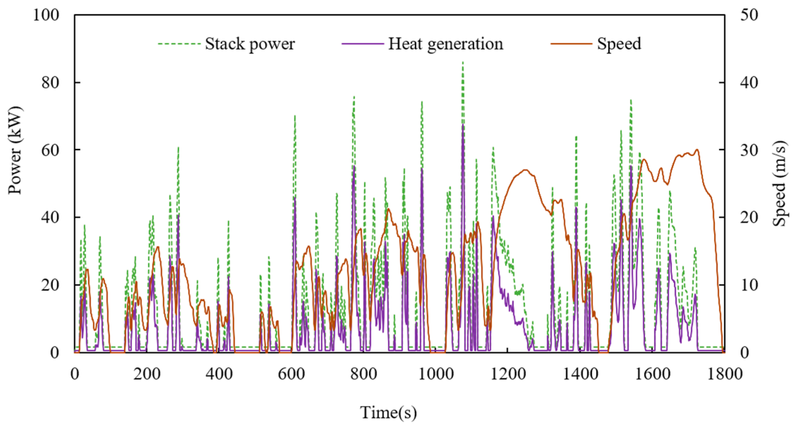
4.2.2. Testing Cycle

The WLTC was selected as the evaluation condition, and the established model was simulated to obtain the variations in stack power, stack heat generation, and vehicle speed, as shown in Figure 10.

5. Results and Discussions

5.1. The Impact of the OOT Tracking Method on PEMFC Systems

To assess the impact of the OOT tracking on PEMFC performance under PID control, stack temperature, average efficiency, and energy consumption were compared between constant-temperature control (80 °C) and OOT tracking methods. Ambient temperature was maintained at 30 °C with a controller sampling interval of 0.5 s. The constant-temperature setpoint (80 °C) represents the median OOT range during cyclic operation. Given the prolonged startup period required for PEMFCs to reach operating temperatures from ambient conditions, the initial system temperature was set to 70 °C. Controller activation commenced when the coolant temperature reached the thermostat’s radiator cycle threshold.

As shown in Figure 11a, prior to reaching the target operating temperature, stack temperatures under both control methods remain low during the warm-up phase. At this stage, the fan remains inactive while the pump operates at baseline speed. Stack operating temperatures are consistent between control strategies until 204 s, when the OOT tracking controller first achieves the target temperature and subsequently adjusts to its variations. In contrast, the thermostatic controller deviates from the OOT trajectory and exceeds optimal values, reducing efficiency relative to OOT tracking. Figure 11b,c demonstrate that OOT tracking increases the average PEMFC efficiency by 1.15% and reduces TMS energy consumption by 7.97%.

5.2. Control Performance of MPC Based on OOT Tracking

Figure 11 demonstrates that OOT tracking enhances PEMFC efficiency while reducing TMS energy consumption. However, Figure 11a reveals significant temperature overshoot under conventional PID control, indicating suboptimal tracking performance. To validate MPC thermal management efficacy, its performance was compared with PID control under WLTC conditions at varying ambient temperatures. Evaluation metrics included OOT tracking accuracy and TMS energy consumption.

5.2.1. Tracking Performance of the OOT

In order to assess the performance of the two control strategies, the root mean square error (RMSE) between the actual temperature of the PEMFC and the target temperature is used as the evaluation metric. The corresponding calculation formula is presented in Equation (45).

$$RMSE=\sqrt{{\displaystyle \frac{1}{N_C}}{\displaystyle \sum _{i=0}^{N_C}{(T_{st(i)}-T_{ref,st(i)})}^2}}$$

(45)

where $N_C$ is the size of the dataset. $T_{st(i)}$ is the simulated value of the stack temperature. $T_{ref,st(i)}$ is the reference value for the stack temperature.

Figure 12 presents the comparative results. When the ambient temperature ($T_{amb}$) is 25 °C, RMSE_MPC is 1.55 °C, and the RMSE_PID is 2.14 °C. When $T_{amb}$ is 40 °C, RMSE_MPC is 1.77 °C, and RMSE_PID is 2.23 °C. When the MPC strategy is implemented, the tracking error of the OOT of the stack is reduced by more than 33%. Unlike PID control—which regulates fan/pump speeds reactively based on $T_{st}$ and $T_{ref,st}$ deviations, introducing dynamic response delays—MPC incorporates predictive state modeling and objective optimization. This enables proactive determination of optimal actuator speeds using real-time feedback, achieving desired system states with reduced transition time.

5.2.2. Energy Consumption Performance of TMS

Figure 13a–d demonstrate that under PID control, pump and fan speeds fluctuate by 5250 rev/min and 4500 rev/min at 25 °C and 40 °C ambient temperatures, respectively. Under MPC at 25 °C, these fluctuations reduce to 3552 rev/min (pump) and 2815 rev/min (fan). At 40 °C, MPC maintains fluctuations at 3980 rev/min (pump) and 3027 rev/min (fan). PID-controlled actuators exhibit significant speed oscillations and response delays, indicating poor synchronization with stack temperature dynamics. Conversely, MPC reduces actuator speed variations through predictive temperature modeling, enabling anticipatory speed adjustments that enhance response rapidity and coordination.

As shown in Figure 14, under WLTC conditions, the TMS with PID control consumes 771,852 J and 880,681 J at 25 °C and 40 °C ambient temperatures, respectively. By contrast, MPC reduces TMS energy consumption to 679,096 J and 762,091 J under identical conditions. This corresponds to energy savings of 10.8% and 12.4% relative to PID control with greater efficacy observed at higher ambient temperatures.

6. Conclusions

This study addresses the high energy consumption challenge in PEMFC TMS for FCVs under high-temperature conditions. We developed a model-adaptive MPC strategy for tracking the OOT to regulate TMS fan and coolant pump operation. Comprehensive analyses of stack temperature control, efficiency, actuator dynamics, and system energy consumption were performed at 25 °C and 40 °C ambient conditions. The main conclusions are as follows:

(1)

In the model validation results, the deviation between experimental data and simulation results of the developed PEMFC and TMS models is within 4%. This indicates that the proposed models possess high accuracy and can effectively support simulation studies.

(2)

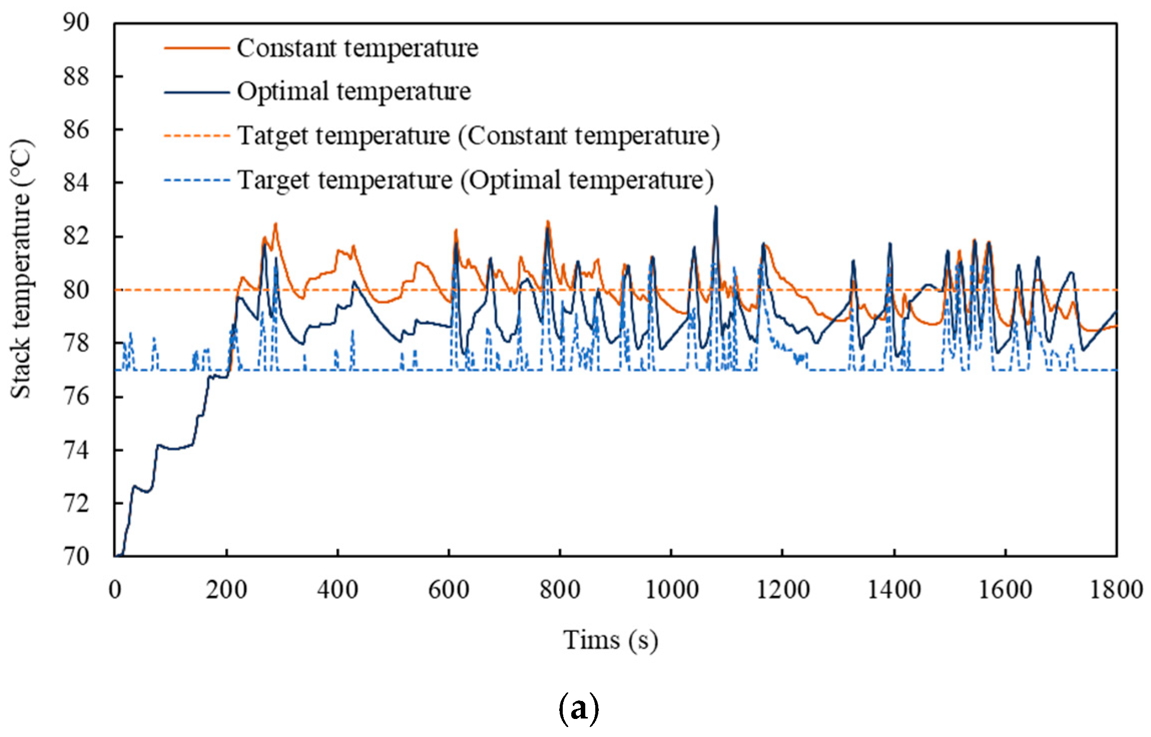
The relationship between the output power of the PEMFC and its OOT was experimentally determined. The OOT corresponding to each output power level was subsequently adopted as the reference trajectory for the controller. In PID control, using the OOT as the reference trajectory (instead of maintaining a constant temperature setpoint) yields a 1.15% improvement in the average efficiency of the PEMFC and a 7.97% reduction in TMS energy consumption.

(3)

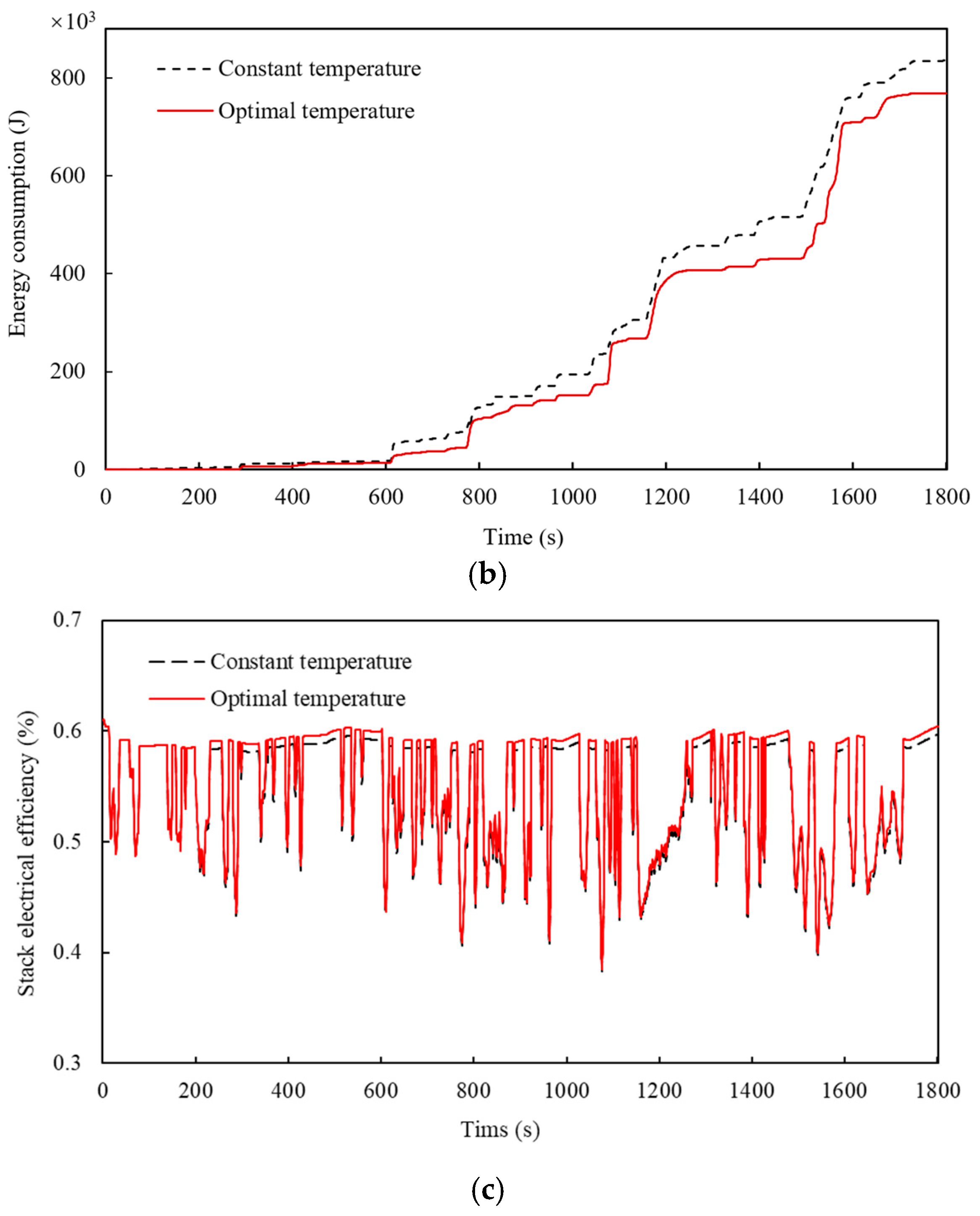
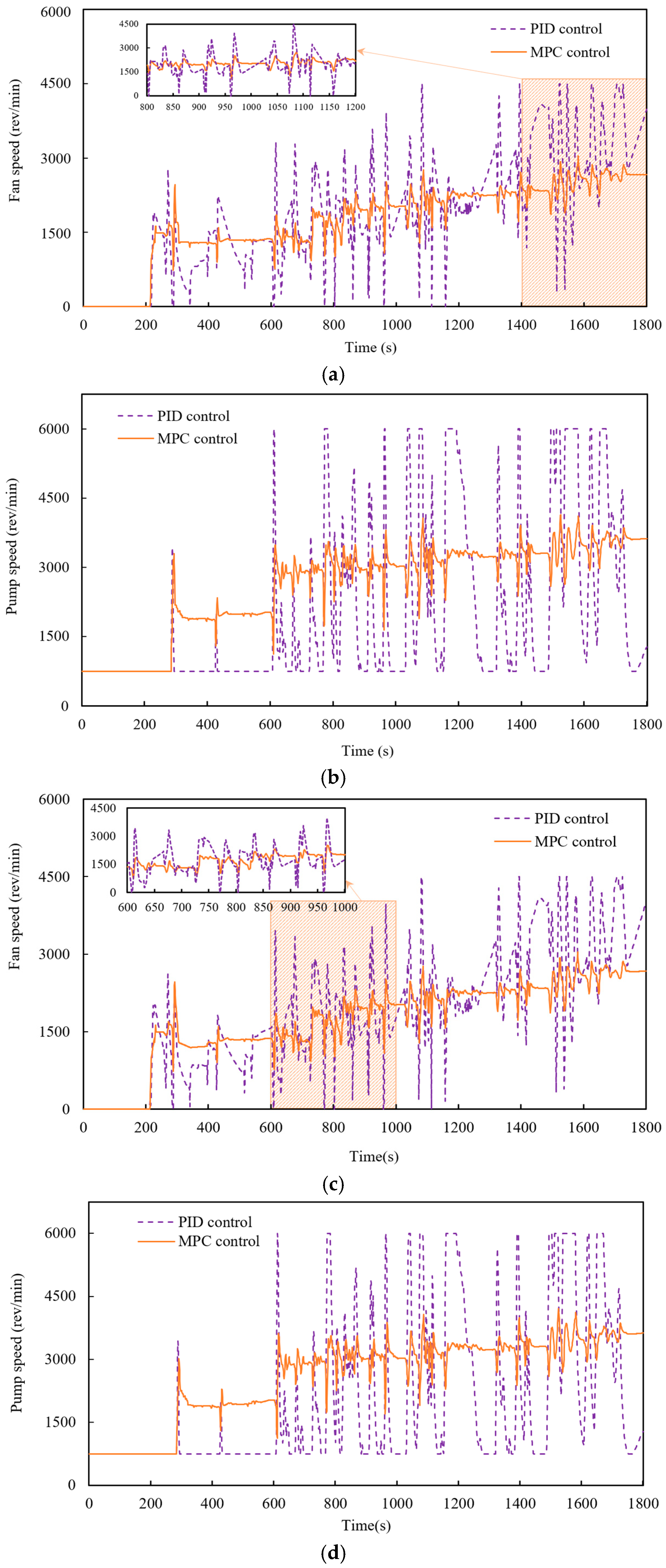
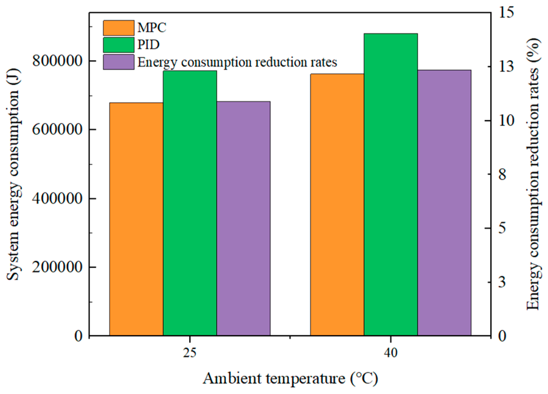
A model-adaptive MPC strategy for OOT tracking is proposed, integrating TMS energy consumption into the objective function to enable multi-objective optimization. Simulation results under the WLTC show that the MPC controller reduces OOT tracking error by more than 33% compared to the PID controller. At 25 °C and 40 °C ambient temperatures, MPC reduces fan speed fluctuations by 37.4% and 32.7%, pump speed fluctuations by 32.3% and 24.2%, and TMS energy consumption by 10.8% and 12.4%, respectively, relative to PID control. Overall, the OOT-tracking-based MPC strategy exhibits higher accuracy and efficiency in regulating fan and pump speeds while achieving lower energy consumption.

Based on the research content and current findings of this study, future research directions may advance through three key dimensions: deepening model investigations, expanding control strategy applications, and optimizing system integration: (1) Advancing modeling techniques: Future work could explore more precise modeling methodologies, such as incorporating stack internal temperature distribution uniformity. Simultaneously, a balance must be struck between model accuracy and computational complexity to ensure real-time performance in practical applications. (2) Multi-objective control optimization: Future control strategies could also incorporate additional objectives, including enhancing the stability of PEMFC output power, extending service life, and reducing system costs, while striking a balance among conflicting objectives. (3) Integrated vehicle system optimization: The TMS for PEMFC does not operate in isolation. Future research should focus on deep integrated optimization between the TMS and other vehicle systems (e.g., powertrain, energy recovery systems, and battery management systems). Synergistic interactions among systems could enable holistic vehicle energy management, thereby elevating the comprehensive performance of FCVs. Furthermore, the implementation of advanced temperature monitoring technologies in the future could enhance measurement accuracy, thereby improving control precision.

References

1. Jia, C.; Liu, W.; He, H.; Chau, K. Health-conscious energy management for fuel cell vehicles: An integrated thermal management strategy for cabin and energy source systems. Energy 2025, 333, 137330–137341. [Google Scholar] [CrossRef]
2. Jia, C.; Liu, W.; He, H.; Chau, K. Superior energy management for fuel cell vehicles guided by improved DDPG algorithm: Integrating driving intention speed prediction and health-aware control. Appl. Energy 2025, 394, 126195–126206. [Google Scholar] [CrossRef]
3. Lu, D.; Yi, F.; Hu, D.; Li, J.; Yang, Q.; Wang, J. Online optimization of energy management strategy for FCV control parameters considering dual power source lifespan decay synergy. Appl. Energy 2023, 348, 121516–121528. [Google Scholar] [CrossRef]
4. Jia, C.; Liu, W.; He, H.; Chau, K. Deep reinforcement learning-based energy management strategy for fuel cell buses integrating future road information and cabin comfort control. Energy Convers. Manag. 2024, 321, 119032–119043. [Google Scholar] [CrossRef]
5. Li, K.; Zhou, J.; Jia, C.; Yi, F.; Zhang, C. Energy sources durability energy management for fuel cell hybrid electric bus based on deep reinforcement learning considering future terrain information. Int. J. Hydrogen Energy 2024, 52, 821–833. [Google Scholar] [CrossRef]
6. Liso, V.; Nielsen, M.; Kaer, S.; Mortensen, H.H. Thermal modeling and temperature control of a PEM fuel cell system for forklift applications. Int. J. Hydrogen Energy 2014, 39, 8410–8420. [Google Scholar] [CrossRef]
7. Saygili, Y.; Eroglu, I.; Kincal, S. Model based temperature controller development for water cooled PEM fuel cell systems. Int. J. Hydrogen Energy 2015, 40, 615–622. [Google Scholar] [CrossRef]
8. Ahn, J.W.; Choe, S.Y. Coolant controls of a PEM fuel cell system. J. Power Sources 2008, 179, 252–264. [Google Scholar] [CrossRef]
9. Chen, J.H.; He, P.; Cai, S.J.; He, Z.-H.; Zhu, H.-N.; Yu, Z.-Y.; Yang, L.-Z.; Tao, W.-Q. Modeling and temperature control of a water-cooled PEMFC system using intelligent algorithms. Appl. Energy 2024, 372, 123790–123809. [Google Scholar] [CrossRef]
10. Cheng, S.; Fang, C.; Xu, L.; Li, J.; Ouyang, M. Model-based temperature regulation of a PEM fuel cell system on a city bus. Int. J. Hydrogen Energy 2015, 40, 13566–13575. [Google Scholar] [CrossRef]
11. Tang, X.; Zhang, Y.; Xu, S. Temperature sensitivity characteristics of PEM fuel cell and output performance improvement based on optimal active temperature control. Int. J. Heat Mass Transf. 2023, 206, 123966–123980. [Google Scholar] [CrossRef]
12. Han, J.; Yu, S.; Yi, S. Advanced thermal management of automotive fuel cells using a model reference adaptive control algorithm. Int. J. Hydrogen Energy 2017, 42, 4328–4341. [Google Scholar] [CrossRef]
13. Song, D.; Wu, Q.; Zeng, X.; Qian, Q.; Yang, D. Feedback-linearization decoupling based coordinated control of air supply and thermal management for vehicular fuel cell system. Energy 2024, 305, 132347–132364. [Google Scholar] [CrossRef]
14. Yan, C.; Chen, J.; Liu, H.; Lu, H. Model-based fault tolerant control for the thermal management of PEMFC systems. IEEE Trans. Ind. Electron 2019, 67, 2875–2884. [Google Scholar] [CrossRef]
15. Chen, X.; Xu, J.; Fang, Y.; Li, W.; Ding, Y.; Wan, Z.; Wang, X.; Tu, Z. Temperature and humidity management of PEM fuel cell power system using multi-input and multi-output fuzzy method. Appl. Therm. Eng. 2022, 203, 117865–117874. [Google Scholar] [CrossRef]
16. Xu, D.; Yan, W.; Ji, N. RBF neural network based adaptive constrained PID control of a solid oxide fuel cell. In Proceedings of the 2016 Chinese Control and Decision Conference (CCDC), Yinchuan, China, 28–30 May 2016; pp. 3986–3991. [Google Scholar]
17. Xu, J.H.; Yan, H.Z.; Ding, Q.; Zhu, K.-Q.; Yang, Y.-R.; Wang, Y.-L.; Huang, T.-M.; Chen, X.; Wan, Z.-M.; Wang, X.-D. Sparrow search algorithm applied to temperature control in PEM fuel cell systems. Int. J. Hydrogen Energy 2022, 47, 39973–39986. [Google Scholar] [CrossRef]
18. Baroud, Z.; Benmiloud, M.; Benalia, A.; Ocampo-Martinez, C. Novel hybrid fuzzy-PID control scheme for air supply in PEM fuel-cell-based systems. Int. J. Hydrogen Energy 2017, 42, 10435–10447. [Google Scholar] [CrossRef]
19. Chen, X.; Feng, W.; You, S.; Hu, Y.; Wan, Y.; Zhao, B. Dual temperature parameter control of PEMFC stack based on improved differential evolution algorithm. Renew. Energy 2025, 241, 122319–122332. [Google Scholar] [CrossRef]
20. Cao, J.H.; Yin, C.; Wang, R.K.; Li, R.; Liu, R.; Tang, H. Dynamic thermal management of proton exchange membrane fuel cell vehicle system using the tube-based model predictive control. Int. J. Hydrogen Energy 2024, 70, 493–509. [Google Scholar] [CrossRef]
21. Tümer, B.; Yıldız, D.Ş.; Arkun, Y. Water and thermal management in PEM fuel cells using feasible humidity plots and model predictive controllers. Comput. Chem. Eng. 2025, 192, 108905–108917. [Google Scholar] [CrossRef]
22. Zhang, Y.Z.; Zhang, C.Z.; Fan, R.J.; Deng, C.; Wan, S.; Chaoui, H. Energy management strategy for fuel cell vehicles via soft actor-critic-based deep reinforcement learning considering powertrain thermal and durability characteristics. Energy Convers. Manag. 2023, 283, 116921–116938. [Google Scholar] [CrossRef]
23. Zhang, Z.; Yuan, W.W.; Wang, Y.X.; Ou, K.; Huang, Y.; Xuan, D. Enhanced deep reinforcement learning-based thermal management strategy for PEMFC considering coolant system parasitic power. Int. J. Hydrogen Energy 2025, 146, 149919–149932. [Google Scholar] [CrossRef]
24. Lin, Y.H.; Huang, Y.H. Integrated thermal and energy management systems using particle swarm optimization for energy optimization in electric vehicles. Case Stud. Therm. Eng. 2025, 71, 106136–106157. [Google Scholar] [CrossRef]
25. Ju, F.; Jiang, Y.H.; Zhuang, W.H.; Li, B.; Dai, J. Integrated optimization of energy management and thermal control strategies for fuel-cell heavy truck. Int. J. Hydrogen Energy 2025, 145, 928–941. [Google Scholar] [CrossRef]
26. Jiang, K.; Tian, Z.; Wen, T.; Song, K.; Hillmansen, S.; Ochieng, W.Y. Collaborative optimization strategy of hydrogen fuel cell train energy and thermal management system based on deep reinforcement learning. Appl. Energy 2025, 393, 2318–2335. [Google Scholar] [CrossRef]
27. Lin, Y.; Lee, M.; Hung, Y. A thermal management control using particle swarm optimization for hybrid electric energy system of electric vehicles. Results Eng. 2024, 21, 101717–101734. [Google Scholar] [CrossRef]
28. De Schepper, P.; Danilov, V.A.; Denayer, J.F.M. Cathode flow field design for nitric oxide/hydrogen fuel cell in cogeneration of hydroxylamine and electricity. Energy Res. 2016, 40, 1355–1366. [Google Scholar] [CrossRef]
29. Luo, X.; Chung, H.S. An Improved MPC-based energy management strategy for hydrogen fuel cell EVs featuring dual-motor coupling powertrain. Energy Convers. Manag. X 2025, 26, 100975–100994. [Google Scholar] [CrossRef]
30. Xie, R.; Ma, R.; Pu, S.; Xu, L.; Zhao, D.; Huangfu, Y. Prognostic for fuel cell based on particle filter and recurrent neural network fusion structure. Energy AI 2020, 2, 100017–100027. [Google Scholar] [CrossRef]
31. Qing, H.Y.; Feng, Y.; Zhang, C.Z.; Gao, J.; Chen, H.; Hao, D.; Yu, P.; Simonovic, M. Parallel structure-based decentralized model predictive control of vehicle PEMFC anode circulation system. Energy 2025, 324, 135767–135779. [Google Scholar] [CrossRef]
32. Deng, Z.; Chen, M.; Wang, H.; Chen, Q. Performance-oriented model learning and model predictive control for PEMFC air supply system. Int. J. Hydrogen Energy 2024, 64, 339–348. [Google Scholar] [CrossRef]
33. Zhu, Y.; Zou, J.; Li, S.; Peng, C.; Xie, Y. Nonlinear model predictive control of PEMFC anode hydrogen circulation system based on dynamic coupling analysis. Int. J. Hydrogen Energy 2023, 48, 2385–2400. [Google Scholar] [CrossRef]
34. Chen, F.X.; Zhang, J.Y.; Pei, Y.W.; Chi, X.; Zhang, H.; Wang, Y. Real-time pressure-flow coordinated control based on adaptive switching algorithm of PEMFC durability test bench. Int. J. Hydrogen Energy 2024, 141, 598–614. [Google Scholar] [CrossRef]
35. Hu, H.; Ou, K.; Yuan, W.W. Fused multi-model predictive control with adaptive compensation for proton exchange membrane fuel cell air supply system. Energy 2023, 284, 128459–128477. [Google Scholar] [CrossRef]
36. He, H.W.; Quan, S.W.; Wang, Y.X. Hydrogen circulation system model predictive control for polymer electrolyte membrane fuel cell-based electric vehicle application. Int. J. Hydrogen Energy 2020, 45, 20382–20390. [Google Scholar] [CrossRef]
37. Zo, W.J.; Kim, Y.B. Temperature control for a 5 kW water-cooled PEM fuel cell system for a household application. IEEE Access 2019, 7, 144826–144835. [Google Scholar] [CrossRef]
38. Masoudi, Y.; Azad, N.L. MPC-based battery thermal management controller for plug-in hybrid electric vehicles. In Proceedings of the 2017 American Control Conference (ACC), Seattle, WA, USA, 24–26 May 2017; pp. 4365–4370. [Google Scholar]
39. Chen, X.; Fang, Y.; Liu, Q.; He, L.; Zhao, Y.; Huang, T.; Wan, Z.; Wang, X. Temperature and voltage dynamic control of PEMFC Stack using MPC method. Energy Rep. 2022, 8, 798–808. [Google Scholar] [CrossRef]
40. Yuan, X.H.; Wu, G.; Zhou, J.G.; Xiong, X.; Wang, Y.-P. MPC-based thermal management for water-cooled proton exchange membrane fuel cells. Energy Rep. 2022, 8, 338–348. [Google Scholar] [CrossRef]
41. Zhang, R.; Jia, Y.; Zhang, T.; Fan, Z. Research on modeling and control of PEMFC cooling system. Appl. Therm. Eng. 2024, 241, 122303–122313. [Google Scholar] [CrossRef]
42. Yang, L.; Nik-Ghazali, N.N.; Ali, M.A.H.; Chong, W.T.; Yang, Z.; Liu, H. A review on thermal management in proton exchange membrane fuel cells: Temperature distribution and control. Renew. Sustain. Energy Rev. 2023, 187, 113737–113756. [Google Scholar] [CrossRef]
43. Yu, X.; Zhou, B.; Sobiesiak, A. Water and thermal management for Ballard PEM fuel cell stack. J. Power Sources 2005, 147, 184–195. [Google Scholar] [CrossRef]
Figure 1. Energy flow diagram of FCVs.
Energies 18 04100 g001
Figure 2. Parameter transfers of the PEMFC thermal management system.
Energies 18 04100 g002
Figure 3. The relationship between speed, flow rate, and power of the pump.
Energies 18 04100 g003
Figure 4. Schematic diagram of the PEMFC experimental platform.
Energies 18 04100 g004
Figure 5. Comparison between simulated and experimental polarization curves of PEMFC under different operational temperatures.
Energies 18 04100 g005
Figure 6. Comparison between simulation and experimental results for heat generation in PEMFC.
Energies 18 04100 g006
Figure 7. Acquisition of the OOT of PEMFC: (a) the relationship between operating temperature and output power; (b) the relationship between output power and OOT.
Energies 18 04100 g007
Figure 8. Schematic diagram of the MPC control process for the PEMFC cooling system.
Energies 18 04100 g008
Figure 9. Co-simulation schematic diagram.
Energies 18 04100 g009
Figure 10. Power and vehicle speed under WLTC condition.
Energies 18 04100 g010
Figure 11. Parameter variations under different control strategies in the WLTC condition: (a) stack temperature; (b) energy consumption of the PEMFC’s TMS; (c) stack electrical efficient.
Energies 18 04100 g011aEnergies 18 04100 g011b
Figure 12. Stack temperature variation under different ambient temperatures: (a) 25 °C; (b) 40 °C.
Energies 18 04100 g012
Figure 13. Fan speed and pump speed variation under different ambient temperatures: (a) fan speed ( T a m b = 25 °C); (b) pump speed ( T a m b = 25 °C); (c) fan speed ( T a m b = 40 °C); (d) pump speed ( T a m b = 40 °C).
Energies 18 04100 g013
Figure 14. Energy consumption of TMS.
Energies 18 04100 g014