Leveraging Dynamic Pricing and Real-Time Grid Analysis: A Danish Perspective on Flexible Industry Optimization

Abstract

Flexibility is advocated as an effective solution to address the growing need to alleviate grid congestion, necessitating efficient energy management strategies for industrial operations. This paper presents a mixed-integer linear programming (MILP)-based optimization framework for a flexible asset in an industrial setting, aiming to minimize operational costs and enhance energy efficiency. The method integrates dynamic pricing and real-time grid analysis, alongside a state estimation model using Extended Kalman Filtering (EKF) that improves the accuracy of system state predictions. Model Predictive Control (MPC) is employed for real-time adjustments. A real-world case studies from aquaculture industries and industrial power grids in Denmark demonstrates the approach. By leveraging dynamic pricing and grid signals, the system enables adaptive pump scheduling, achieving a 27% reduction in energy costs while maintaining voltage stability within 0.95–1.05 p.u. and ensuring operational safety. These results confirm the effectiveness of grid-aware, flexible control in reducing costs and enhancing stability, supporting the transition toward smarter, sustainable industrial energy systems.

1. Introduction

The increasing integration of renewable energy sources and price-responsive consumers driven by the goal of achieving a carbon-free society by 2050 [1] has led to greater uncertainty and variability in power systems, thereby intensifying the need for sufficient flexibility. Flexibility provision approaches can generally be categorized into three main parts: demand-side, generation-side, and storage-based solutions [2]. However, emerging technologies that create links between the power sector and other domains such as water pumps underscore the growing importance of sector coupling as a source of flexibility. In this context, the optimal operation of water pumping systems in industrial clusters near water from the sea not only provides valuable flexibility to the power system but also presents an opportunity for profit maximization. Therefore, it is crucial to explore how the optimal energy management of such systems can be implemented, taking into account the technical constraints of the power grid and the accurate state estimation of water levels.

In recent years, several studies have investigated the optimal energy management of the water–energy nexus. The authors of [3] developed a mixed-integer nonlinear programming model for the day-ahead scheduling of integrated water and power systems, incorporating flexible components such as variable-speed pumps. Their results demonstrated a 4.6% reduction in operational costs compared to the case where the two systems are optimized independently. The authors of [4,5] analyzed the optimal energy mix for water-pumping systems, comparing renewable and non-renewable sources alongside demand-response flexibility. According to the results, a hybrid setup of biomass-based distributed generation, photovoltaics, and time-of-use demand response minimizes cost; applying the Generalized Reduced Gradient nonlinear optimization yields energy costs of 0.018 USD/kWh (with carbon tax) and 0.016 USD/kWh (without).

The impact of a water distribution network comprising multiple pumps and tanks on the optimal day-ahead scheduling of the power system was analyzed in [6] using a mixed-integer linear programming approach. A flexible power-water flow model was introduced in [7] to optimize the scheduling of energy-intensive assets in water systems, such as water treatment and desalination plants, as well as variable-speed pumps and tanks, thereby highlighting their contribution to power system flexibility. Due to the strong interdependence between water distribution grids and power systems, largely stemming from the prevalence of variable-speed pumps, a nonlinear conjunctive optimization model was developed in [8], which achieved a 10% reduction in total system costs. In the context of smart energy communities, ref. [9] introduced a water–energy nexus model aimed at minimizing the community’s operating costs. The model used integer variables to capture the on/off status of pumps, and the results confirmed its superior cost efficiency compared to separately optimizing each sector. In [10], a hardware-in-the-loop testbed for a water distribution system was employed to validate a real-time economic dispatch model for integrated energy and water systems. The study also utilized machine learning techniques to solve the optimization problem efficiently.

Researchers have proposed strategies to optimize integrated water–electricity systems. A three-step approach improved computational efficiency, cutting curtailment and operational costs by over 50% [11]. Optimal tank design and joint energy–water storage enhanced flexibility and water quality [12,13], while a robust data-driven model improved peak load handling and uncertainty management [14]. Transfer delay modeling using electrical–water analogies also supported wind integration [15]. Solar-powered pumping with battery storage improved control performance [16], and standalone PV systems enabled crisis-resilient water supply [17]. Smart meters and 5G supported real-time pump energy reduction and water quality assurance [18]. An integrated nexus model showed the role of water storage in energy planning [19]. Metaheuristic optimization minimized pump energy use while maintaining water standards [20]. IoT-enabled smart tanks enhanced monitoring, leakage detection, and control [21]. Based on a Neuro fuzzy logic algorithm, optimal energy management of the system of batteries and wind turbines for supplying water pumping has been suggested in [22]. Additionally, in [23], the authors proposed a Takagi–Sugeno fuzzy model for the optimal energy management of a hybrid system that consists of a photovoltaic system, a wind turbine, and a battery for supplying water to a rural region without access to the main grid. A mixed integer nonlinear programming approach was proposed in [24] for optimizing the management of water and energy integration as a virtual power plant model for an irrigation system. A machine-learning-based optimal pump operation scheduling model was proposed in [25], taking into account dynamic load fluctuations, electricity prices, and the technical constraints of the system. An economic model predictive model was proposed in [26] for estimating the optimal scheduling for seawater pumping systems, utilizing demand-side management, batteries, and solar energy for load shifting as well as peak shaving. For convenience,

Table 1. Comparison of state-of-the-art studies with this work.

Paper (Ref.)	Optimisation/Control Method	Closed-Loop	Grid-Voltage	Price/DR	Storage Modelled	Experimental/ Validation
[3]	MINLP, day-ahead co-optimization	—	—	✓	Water tanks	—
[4]	Hybrid PV/wind sizing	—	—	✓	Battery	—
[5]	Conceptual flexibility model	—	—	✓	Water tanks	—
[6]	MILP, day-ahead scheduling	—	—	✓	Water tanks	—
[7]	MILP, day-ahead scheduling	—	—	✓	Water tanks	—
[8]	Nonlinear conjunctive optimization	—	—	✓	Water tanks	—
[9]	MILP, micro WEN	—	—	✓	Battery + tanks	—
[10]	Data-driven economic dispatch	∼	—	✓	Tanks	HIL bench
[11]	Three-step cost minimization	—	—	✓	Tanks	—
[12]	Tank-size optimization	—	—	—	Water tanks	—
[13]	Joint electricity–water storage sizing	—	—	—	Battery + tanks	—
[14]	Two-stage robust optimization	—	—	✓	Battery + tanks	—
[15]	Delay-aware scheduling	—	—	✓	Tanks	—
[16]	MPC for PV-pump	∼	—	—	Battery	Lab
[17]	Stand-alone PV sizing	—	—	—	Battery	Field (crisis)
[18]	MILP with water-quality limits	—	—	✓	Tanks	—
[19]	Integrated E-W-F resource planning	—	—	—	Water storage	—
[20]	Meta-heuristic pump scheduling	—	—	✓	—	—
[21]	IoT monitoring/control	—	—	—	—	Prototype
[22]	Neuro-fuzzy EMS	∼	—	—	Battery	—
[23]	Takagi–Sugeno EMS	∼	—	—	Battery	—
[24]	MINLP virtual power plant	—	—	✓	Battery	—
[25]	ML pump scheduling	—	—	✓	—	—
[26]	Economic MPC, seawater pumps	∼	—	✓	Battery	Simulation
This Paper	MILP + EKF + MPC	✓	✓	✓	Water Tank	Industrial field data

✓ Feature is included in the study. ∼ Partially addressed or limited support.

is presented below to compare our proposed work with state-of-the-art studies.

While prior demand-response research within the water–energy nexus has predominantly focused on either economic scheduling or advanced control and monitoring, few studies have addressed a fully integrated, real-time, closed-loop architecture that combines both aspects. This paper proposes and validates a closed-loop, grid-aware energy management scheme for an industrial saltwater pumping facility in Denmark. The proposed method consists of three key steps: First, an EKF reconstructs tank levels, flow rates, and busbar voltage from noisy or incomplete SCADA data. Then, in the second step, a mixed-integer linear programming (MILP) model is developed to co-optimize pump on/off schedules based on 24 h electricity price forecasts, incorporating both hydraulic and voltage-band constraints. Finally, in the third step, a hourly receding-horizon MPC layer continuously updates and resolves the MILP using the latest state estimates. The main contributions of this study are as follows:

• The objective function incorporates quadratic penalties on deviations from real-time EKF state estimates, ensuring that the economic optimizer does not propose hydraulically or electrically infeasible actions even in the presence of sensor drift or failure.
• Voltage-band constraints are co-optimized alongside pump operations, transforming the water process from a passive price-taker into an active asset within the distribution grid.
• A unified linearized model simultaneously represents tank mass balances and nodal voltage behavior, enabling integration of hourlyl optimization with second-level dynamic simulation.

The remainder of the paper is structured as follows: Section 2 describes the methodological framework and the Danish industrial saltwater pumping case study, including the integration of dynamic electricity pricing and real-time grid analysis. Section 3 elaborates the mathematical formulation, highlighting how the MILP model and EKF are employed to enable real-time state estimation and grid-aware scheduling. Section 4 presents simulation results, highlighting cost savings, voltage stability, and system flexibility, and illustrates the model’s potential for active industrial participation in smart grid operations. Section 5 concludes with key findings.

2. Materials and Methods

The primary objective of this study is to optimize the operational strategy of a saltwater distribution system located in Denmark, in order to minimize both energy consumption and operational costs while simultaneously ensuring system flexibility and grid stability. This Danish case study exemplifies the nation’s progressive approach toward sustainable and smart industrial energy use. The optimization strategy is achieved through the integration of advanced state estimation techniques—specifically the EKF—to accurately estimate real-time water flow rates and tank levels. Furthermore, the optimization framework incorporates real-time electricity pricing signals, enabling the system to dynamically adjust pump operations in response to grid demands, thus supporting Denmark’s broader goals for intelligent demand-side management.

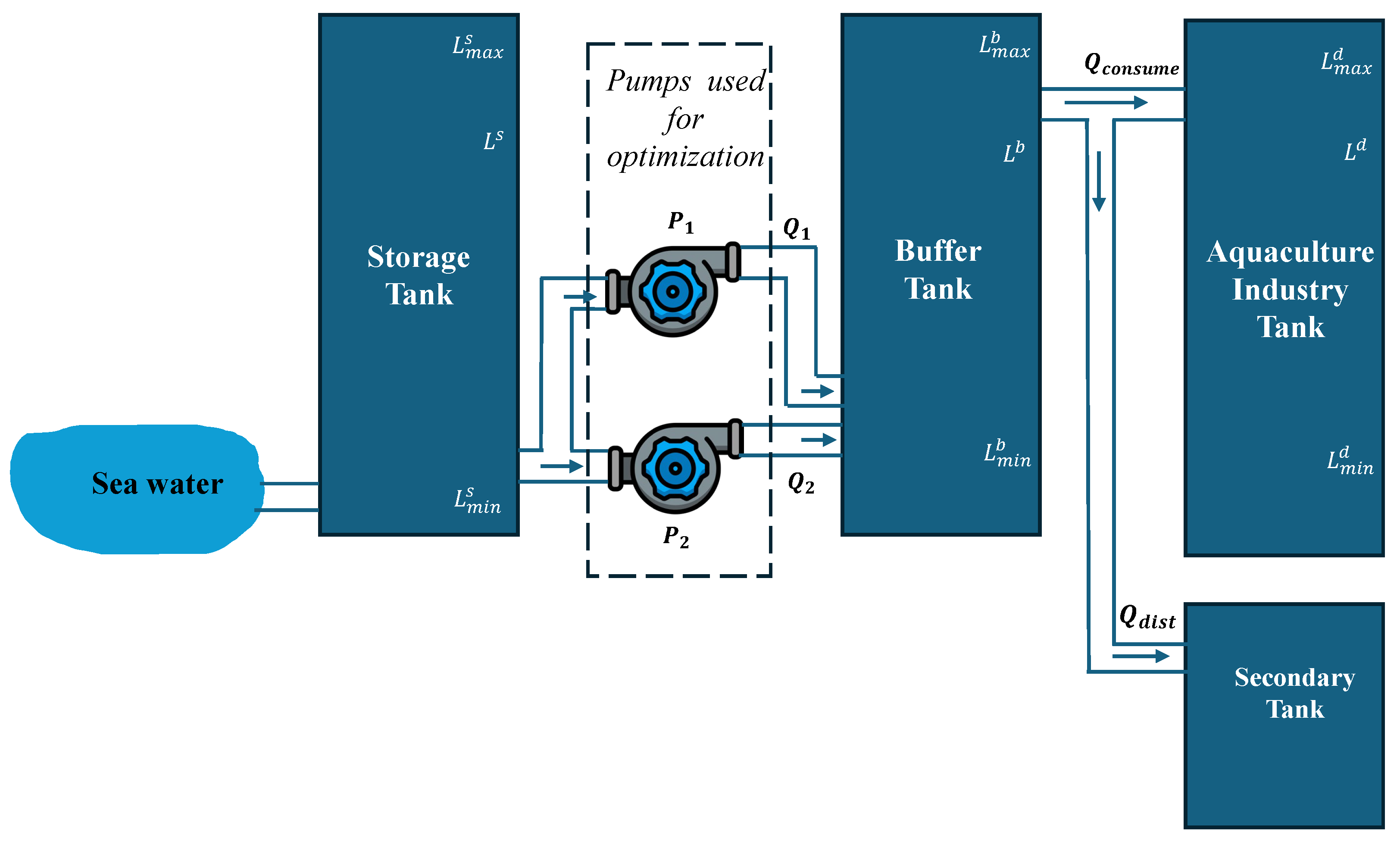
2.1. Description of Saltwater Distribution System

The saltwater distribution network comprises four interconnected tanks designed to supply water from the sea to an industrial aquaculture facility. The saltwater distribution network used in this study is shown in Figure 1. The system’s flexibility and control responsiveness are evaluated based on this configuration, which serves as a representative example of Denmark’s potential for integrated water–energy optimization in coastal industries.

Tank 1, designated as the storage tank, serves as the primary reservoir, collecting water directly from the sea. The water level in this tank varies according to gravitational inflows influenced by tidal conditions.

Tank 2, referred to as the buffer tank, is supplied with saltwater from the storage tank via two electrically driven centrifugal pumps. Each pump has a rated capacity of 250 ${\mathrm{m}}^3$/h and consumes 22.5 kWh under full operational load. The buffer tank serves as an intermediary node, regulating water flow to downstream units while mitigating flow variability.

Tank 3, identified as the aquaculture industry tank, receives water exclusively from the buffer tank. This tank supplies the aquaculture process directly, thus maintaining a continuous and stable inflow that is essential to prevent operational disturbances in the industrial system.

In parallel, a secondary tank is also connected to the buffer tank. This unit has a relatively constant water demand, maintained within the range of 15 to 20 ${\mathrm{m}}^3$/h throughout the operational period. Furthermore, the aquaculture industry tank and secondary tanks are modeled as fixed-load units with time-dependent water consumption profiles. Their demand is treated as an external input, rather than an optimization variable.

2.2. Optimization Framework of Saltwater Distribution System

To minimize energy costs while ensuring safe and reliable operation, we propose an optimization framework that jointly optimizes pump scheduling and water flow dynamics in a saltwater distribution system. The framework integrates MILP for pump scheduling (see Equation (1)), EKF for real-time state estimation of critical variables such as tank water levels (${\widehat{L}}_b\left(t\right),{\widehat{L}}_s\left(t\right),{\widehat{L}}_d\left(t\right)$), flow rates (${\widehat{Q}}_1\left(t\right),{\widehat{Q}}_2\left(t\right)$), and voltage magnitude ($\widehat{V}\left(t\right)$) (Equations (17)–(20)), and MPC for closed-loop control that adapts to disturbances and future system behavior using the estimated states and optimized trajectories (Equation (16)).

The optimization process is constrained by a set of operational and physical limitations to ensure safe and efficient system performance. These include the enforcement of minimum and maximum allowable water levels for each tank (buffer: $L_b\left(t\right)$, storage: $L_s\left(t\right)$, aquaculture: $L_d\left(t\right)$) to prevent overflow or dry-out conditions (Equations (5)–(7), as well as adherence to pump capacity limits and ramping constraints ($Q_1\left(t\right)$, $Q_2\left(t\right)$, $P_i\left(t\right)$) (Equations (8), (9), (12) and (13)).

Additionally, the framework incorporates real-time electricity pricing signals $\lambda \left(t\right)$ that vary dynamically over the optimization horizon, allowing for cost-effective scheduling. Mass balance equations are also applied to govern the inflow and outflow dynamics at each tank node, ensuring hydraulic consistency across the distribution network (Equations (2)–(4)).

For each time step, the EKF first estimates the current system states. These estimates are then passed to the MILP module, which computes the optimal pumping schedule. Finally, the MPC utilizes the MILP-generated trajectories and EKF outputs to determine and issue control actions ($P_1\left(t\right),P_2\left(t\right)$) for the next time interval, ensuring closed-loop implementation and adherence to system constraints (Equation (16)).

To assess the effectiveness of the proposed optimization and control architecture, two simulation scenarios are considered. In the first, a baseline case is implemented, representing business-as-usual operation with static pump schedules and no real-time optimization. In contrast, the optimized scenario incorporates the full integration of MILP-based scheduling, EKF-based state estimation, and MPC for dynamic real-time control. The MILP problem is formulated and implemented using the Pyomo optimization framework and solved using the open-source CBC (Coin-or branch-and-cut) solver, enabling a practical evaluation of the model’s performance in achieving cost efficiency, voltage stability, and operational flexibility under real-world conditions. The Algorithm 1 and the mathematical equations used in the algorithm are given below.

Algorithm 1 MPC Optimization Framework with EKF and MILP

1: Input: Time-series SCADA data: $P_{1\_meas}\left(t\right)$, $P_{2\_meas}\left(t\right)$, tank inflows/outflows, $Q_{consume}\left(t\right)$, $Q_{dist}$, voltage readings, electricity prices   2: Output: Optimized control actions: $P_1\left(t\right)$, $P_2\left(t\right)$, $Q_1\left(t\right)$, $Q_2\left(t\right)$, $L_b\left(t\right)$, $L_s\left(t\right)$, $L_d\left(t\right)$, $V\left(t\right)$, $E\left(t\right)$, $C\left(t\right)$ State Estimation via EKF   3: Initialize EKF state vector: $$X\left(0\right)={[L_b\left(0\right),L_s\left(0\right),L_d\left(0\right),V\left(0\right),{\dot{L}}_b\left(0\right),{\dot{L}}_s\left(0\right),{\dot{L}}_d\left(0\right),\dot{V}\left(0\right)]}^{\top }$$   4: for each time step t do   5:       Predict next state: $X(t+1|t)=AX(t)+BU(t)$   6:       Update using measurements: $Y\left(t\right)=CX\left(t\right)+W\left(t\right)$   7:       Output estimated states: ${\widehat{L}}_b\left(t\right)$, ${\widehat{L}}_s\left(t\right)$, ${\widehat{L}}_d\left(t\right)$, $\widehat{V}\left(t\right)$   8: end for MPC Optimization using MILP   9: for each control interval $t=1$ to T do 10:       Define decision variables: Pump setpoints: $P_1\left(t\right),P_2\left(t\right)\in [0,100]$ Flow rates: $Q_1\left(t\right),Q_2\left(t\right)$ Tank volumes/levels: $V_b,V_s,V_d$, $L_b,L_s,L_d$ Reactive power: $Q_{\mathrm{reactive}}\left(t\right)$ Optimized voltage $V\left(t\right)$ Energy: $E\left(t\right)$, Cost: $C\left(t\right)$ 11:       Add constraints: $Q_i={\displaystyle \frac{P_i}{100}}·Q_{\max }$ Tank mass balances from flow dynamics Level-volume relations: $L_x={\displaystyle \frac{V_x}{A_x/V_x}}$ for each tank Estimated voltage: $\widehat{V}\left(t\right)$ included directly Voltage limits: $0.95\le V\left(t\right)\le 1.05$ Runtime and ramp constraints on $P_1$, $P_2$ 12:       Minimize objective: $$\begin{array}{l}\min [C\left(t\right)+\alpha ·E\left(t\right)+{\beta }_b·z_b\left(t\right)+{\beta }_s·z_s\left(t\right)\\ +{\beta }_d·z_d\left(t\right)+\delta ·z_v\left(t\right)]\hspace{1em}\hspace{1em}\hspace{1em}\hspace{1em} \end{array}$$ 13:       Solve MILP and apply control actions 14: end for 15: Return: Optimized control trajectories and predicted states

3. Mathematical Formulation for MILP and EKF

Building on the system architecture and optimization framework presented in Section 2, the following section formalizes the mathematical foundation used to implement MILP and EKF for real-time grid-aware energy management.

3.1. Mathematical Integer Linear Programming

The objective of the MILP (Equation (1)) is to minimize the total operational cost while ensuring energy efficiency, demand fulfilment, and grid stability. To reflect the Model Predictive Control (MPC) structure used in this study, the complete cost over the prediction horizon is formulated as

$$min\sum _{t=t_0}^{t_0+T}[C\left(t\right)+\alpha ·E\left(t\right)+{\beta }_b·z_b\left(t\right)+{\beta }_s·z_s\left(t\right)+{\beta }_d·z_d\left(t\right)+\delta ·z_v\left(t\right)]$$

(1)

Here, T denotes the time horizon and the auxiliary variables $z_b\left(t\right),z_s\left(t\right),z_d\left(t\right),z_v\left(t\right)$ approximate the squared deviations:

$$z_b\left(t\right)\approx {({\widehat{L}}_b\left(t\right)-L_b\left(t\right))}^2,\mathrm{and}\mathrm{similarly}\mathrm{for}{z}_s\left(t\right),z_d\left(t\right),z_v\left(t\right)$$

represent the linearized deviations used to maintain MILP tractability. Equation (1) corresponds to the objective evaluated at a single time step t and is solved in a receding-horizon fashion across the window $[t_0,t_0+T]$ at each control interval.

• $C\left(t\right)$: Operational cost at time step t, computed based on energy consumption and electricity price.
• $E\left(t\right)$: Total energy consumed at time t, derived from pump operation decisions.
• ${\widehat{L}}_b\left(t\right)$, ${\widehat{L}}_s\left(t\right)$, ${\widehat{L}}_d\left(t\right)$: Estimated water levels of the buffer tank, storage tank, and aquaculture tank at time t, respectively.
• $L_b\left(t\right)$, $L_s\left(t\right)$, $L_d\left(t\right)$: Optimized decision variables for tank levels at time t.
• $\widehat{V}\left(t\right)$: Estimated voltage at time t.
• $V\left(t\right)$: Optimized voltage decision variable at time t.
• $\alpha$: Weighting coefficient for energy consumption.
• ${\beta }_b$, ${\beta }_s$, ${\beta }_d$: Weighting coefficients for the buffer, storage, and aquaculture tank level deviations, respectively.
• $\delta$: Weighting coefficient for voltage deviation penalty.

1.

Mass Balance Constraints are given in Equations (2)–(4).

$$\begin{array}{cc}{Q}_1\left(t\right)-\left(Q_2\left(t\right)+Q_{\mathrm{dist}}\left(t\right)\right)\hfill & ={\displaystyle \frac{V_{\mathrm{buffer}}(t+1)-V_{\mathrm{buffer}}\left(t\right)}{\Delta t}}\hfill \end{array}$$

(2)

$$\begin{array}{cc}{Q}_2\left(t\right)-Q_{\mathrm{consume}}\left(t\right)\hfill & ={\displaystyle \frac{V_{\mathrm{Aquaculture}}(t+1)-V_{\mathrm{Aquaculture}}\left(t\right)}{\Delta t}}\hfill \end{array}$$

(3)

$$\begin{array}{cc}{Q}_{\mathrm{dist}}\left(t\right)\hfill & ={\displaystyle \frac{V_{\sec }(t+1)-V_{\sec }\left(t\right)}{\Delta t}}\hfill \end{array}$$

(4)

• $V_{\mathrm{buffer}}\left(t\right)$, $V_{\mathrm{Aquaculture}}\left(t\right)$, $V_{\sec }\left(t\right)$: Water volumes in buffer, aquaculture, and secondary tanks.
• $Q_{\mathrm{dist}}\left(t\right)$, $Q_{\mathrm{consume}}\left(t\right)$: Outflow from secondary stream and demand from aquaculture.

2.

The Water Level Constraints are given in Equations (5)–(7).

$$\begin{array}{c}{L}_{min}^b\le L_b\left(t\right)\le L_{max}^b\hfill \end{array}$$

(5)

$$\begin{array}{c}{L}_{min}^s\le L_s\left(t\right)\le L_{max}^s\hfill \end{array}$$

(6)

$$\begin{array}{c}{L}_{min}^d\le L_d\left(t\right)\le L_{max}^d\hfill \end{array}$$

(7)

• $L_b\left(t\right)$, $L_s\left(t\right)$, $L_d\left(t\right)$: Water levels at time t for buffer, storage, and aquaculture tanks.
• $L_{min}^x$, $L_{max}^x$: Minimum and maximum allowable levels.

3.

The Pump Constraints are given in Equations (8) and (9).

$$\begin{array}{c}0\le Q_1\left(t\right),Q_2\left(t\right)\le Q_{\max }\hfill \end{array}$$

(8)

$$\begin{array}{c}{P}_i\left(t\right)\in \{0,1\},\forall i\in \{1,2\}\hfill \end{array}$$

(9)

$Q_{\max }$: Maximum pump flow rate.

4.

The Energy Consumption Calculation is given in Equation (10).

$$\begin{array}{c}E\left(t\right)=\sum _{i=1}^2{P}_i\left(t\right)·E_{\mathrm{unit}}\hfill \end{array}$$

(10)

$E_{\mathrm{unit}}$: Energy consumption per pump operation.

5.

The Energy Efficiency Constraints are given in Equations (11)–(13).

$$\begin{array}{cc}{Q}_i\left(t\right)\hfill & \ge Q_{min}·P_i\left(t\right),\forall i\in \{1,2\},\forall t\hfill \end{array}$$

(11)

$$\begin{array}{cc}{s}_i\left(t\right)\hfill & \ge P_i\left(t\right)-P_i(t-1),s_i\left(t\right)\ge P_i(t-1)-P_i\left(t\right),s_i\left(t\right)\le S_{max}\hfill \end{array}$$

(12)

$$\begin{array}{cc}\sum _{k=t}^{t+T_{\min }}{P}_i\left(k\right)\hfill & \ge T_{\min }·P_i\left(t\right),\forall i\in \{1,2\}\hfill \end{array}$$

(13)

• $Q_i\left(t\right)$: Flow from pump i, linearly dependent on binary state.
• $s_i\left(t\right)$: Auxiliary variable to linearize switching constraint.
• $Q_{min}$: Minimum flow when pump is active.
• $T_{min}$: Minimum runtime once activated.
• $S_{max}$: Max switching rate between time steps.

6.

The Energy Consumption and Cost Constraints are given in Equations (14) and (15).

$$\begin{array}{cc}C\hfill & =\sum _{t}E\left(t\right)·\left(\lambda \left(t\right)+{\lambda }_{\mathrm{transp}}\left(t\right)\right)\hfill \end{array}$$

(14)

$$\begin{array}{cc}{Q}_1\left(t\right)+Q_2\left(t\right)\hfill & \le Q_{\max }\hfill \end{array}$$

(15)

Conditions: If $\lambda \left(t\right)\le {\lambda }_{\mathrm{low}}$ and if $\lambda \left(t\right)\ge {\lambda }_{\mathrm{peak}}$ are handled using binary variables and logic constraints (not written here due to MILP scope). Here, ${\lambda }_{\mathrm{low}}$ is the threshold for low-price classification and ${\lambda }_{\mathrm{peak}}$ is the threshold for peak-price classification

• $\lambda \left(t\right)$: Electricity price at time t.
• ${\lambda }_{\mathrm{transp}}\left(t\right)$: Transmission price at time t.
• C: Total cost of electricity consumption.
• $Q_{\max }$: Max combined flow rate.

7.

The Voltage Constraints for grid stability are given in Equation (16).

$$\begin{array}{c}{V}_{\min }\le V\left(t\right)\le V_{\max },\forall t\hfill \end{array}$$

(16)

• $V_{min},V_{max}$: Permissible voltage limits (e.g., 0.95–1.05 p.u.).
• $V\left(t\right)$: Voltage at time t.

3.2. State Estimation via EKF

1.

The State Transition Model Equations are given in Equations (17)–(19).

$$\begin{array}{cc}X(t+1)\hfill & =AX\left(t\right)+BU\left(t\right)+W\left(t\right),W\left(t\right)\sim \mathcal{N}(0,Q)\hfill \end{array}$$

(17)

$$\begin{array}{cc}X\left(t\right)\hfill & =\left[\begin{array}{c}{\widehat{L}}_b\left(t\right)\\ {\widehat{Q}}_1\left(t\right)\\ {\widehat{Q}}_2\left(t\right)\end{array}\right]\hfill \end{array}$$

(18)

$$\begin{array}{cc}U\left(t\right)\hfill & =\left[\begin{array}{c}{P}_1\left(t\right)\\ P_2\left(t\right)\end{array}\right]\hfill \end{array}$$

(19)

2.

The Measurement Model is given in Equation (20).

$$\begin{array}{cc}Y\left(t\right)\hfill & =CX\left(t\right)+M\left(t\right),M\left(t\right)\sim \mathcal{N}(0,R)\hfill \end{array}$$

(20)

• $X\left(t\right)$ represents the estimated state variables (buffer tank level and pump flow rates).
• $U\left(t\right)$ represents the control inputs (pump activation).
• $W\left(t\right)$ and $M\left(t\right)$ represent process and measurement noise, respectively.

The system matrices are defined as follows:

• $A\in {\mathbb{R}}^{n\times n}$: State transition matrix describing the evolution of water levels and voltage.
• $B\in {\mathbb{R}}^{n\times m}$: Control input matrix mapping pump actions to state changes.
• $C\in {\mathbb{R}}^{p\times n}$: Observation matrix mapping system states to measured outputs.

The exact values of these matrices were derived from linearization of the physical dynamics around nominal operating points. The noise covariance matrices $Q\in {\mathbb{R}}^{n\times n}$ and $R\in {\mathbb{R}}^{p\times p}$ model process and measurement uncertainties, respectively.

The process noise covariance matrix Q and the measurement noise covariance matrix R were calibrated based on historical SCADA data variability. Specifically, Q was tuned to reflect slow changes in tank levels and voltage, while R was selected based on sensor accuracy specifications and empirical measurement noise distributions. A sensitivity analysis confirmed that these values offered stable convergence and reliable estimation performance under typical operating conditions.

Although the system exhibits mild nonlinearities, the Extended Kalman Filter (EKF) was selected for its computational simplicity and real-time feasibility within industrial controllers. In our tests, the EKF produced stable and accurate estimates under typical load conditions. Nevertheless, for systems with stronger nonlinearities or fast dynamics, an Unscented Kalman Filter (UKF) could offer performance advantages. We highlight this as a direction for future work.

4. Simulation Results

4.1. Economic Benefits of Dynamic Pricing

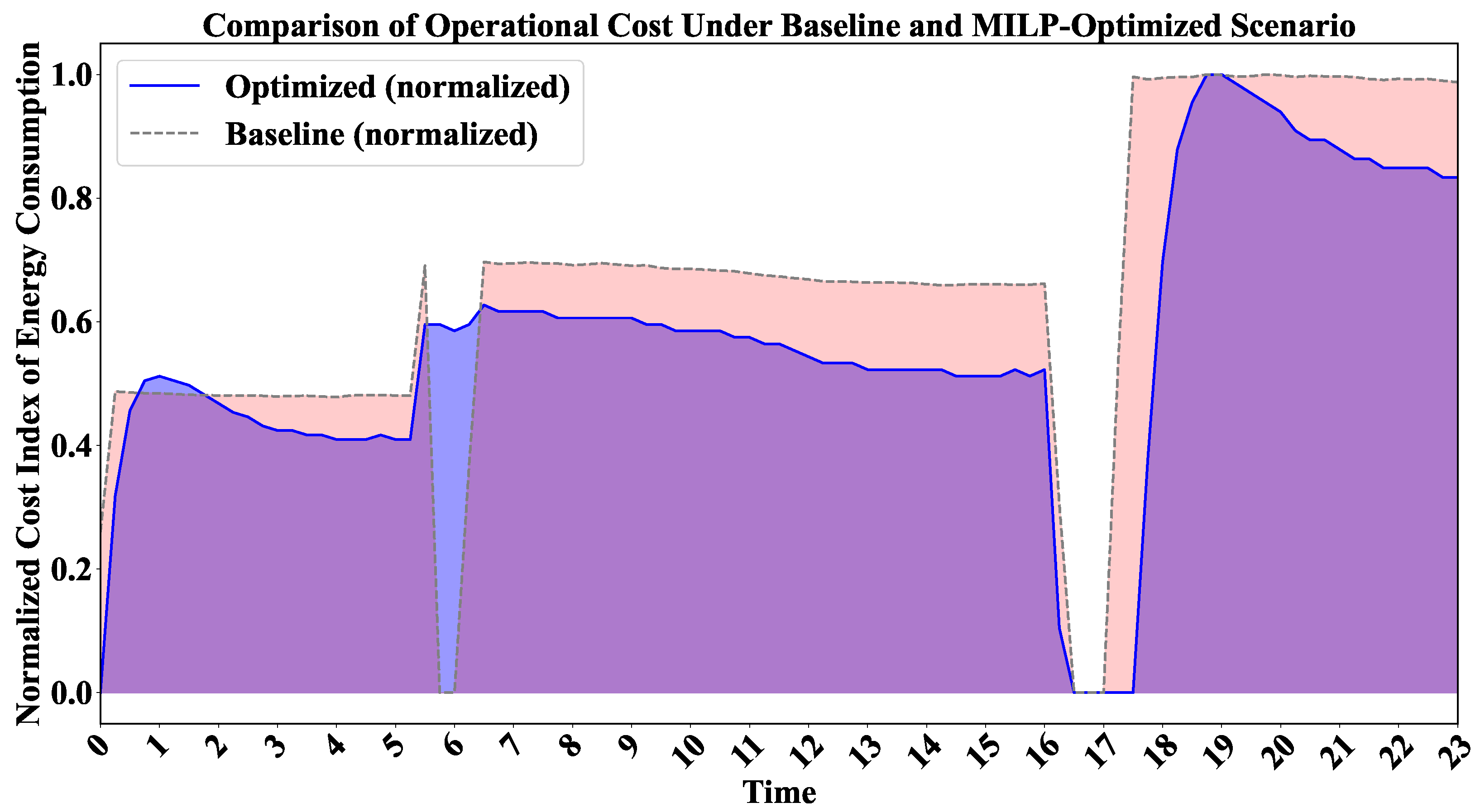
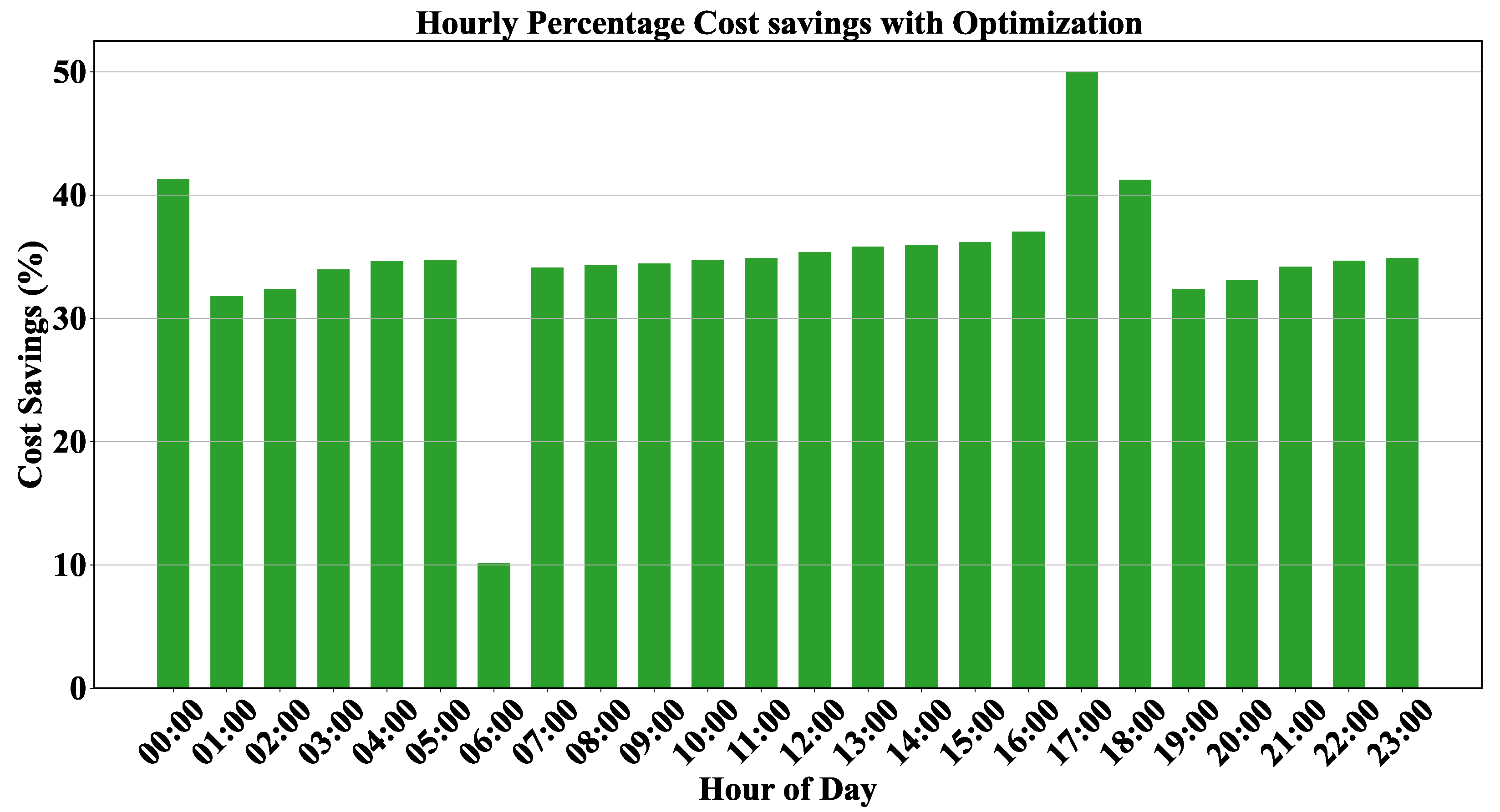
4.1.1. Cost Dynamics Under Time-Variant Electricity Pricing

Figure 2 illustrates a 27% reduction in normalized energy cost achieved through MILP optimization. Pump operations are scheduled during low-tariff periods (electricity price $\lambda \left(t\right)\le 1.66$ øre/kWh $+6.1$ øre/kWh) [27,28], while fulfilling the aquaculture tank demand and maintaining grid voltage within 0.95–1.05 p.u. The cost savings are computed by comparing the total energy cost of the system under optimized operation to that of the baseline, using a normalized cost index over a 24 h period. This demonstrates the economic advantage of dynamic pricing over the baseline scenario.

To further characterize cost efficiency, Figure 3 presents the hourly percentage cost savings resulting from the optimized schedule. Savings range from 12% to 48%, with the maximum reduction observed between 01:00 and 06:00—a period coinciding with off-peak tariffs. The schedule maintains system constraints, ensuring a continuous inflow rate of 250 ${\mathrm{m}}^3$/h and voltage stability within 0.95–1.05 p.u., thereby validating the temporal economic effectiveness of dynamic pricing.

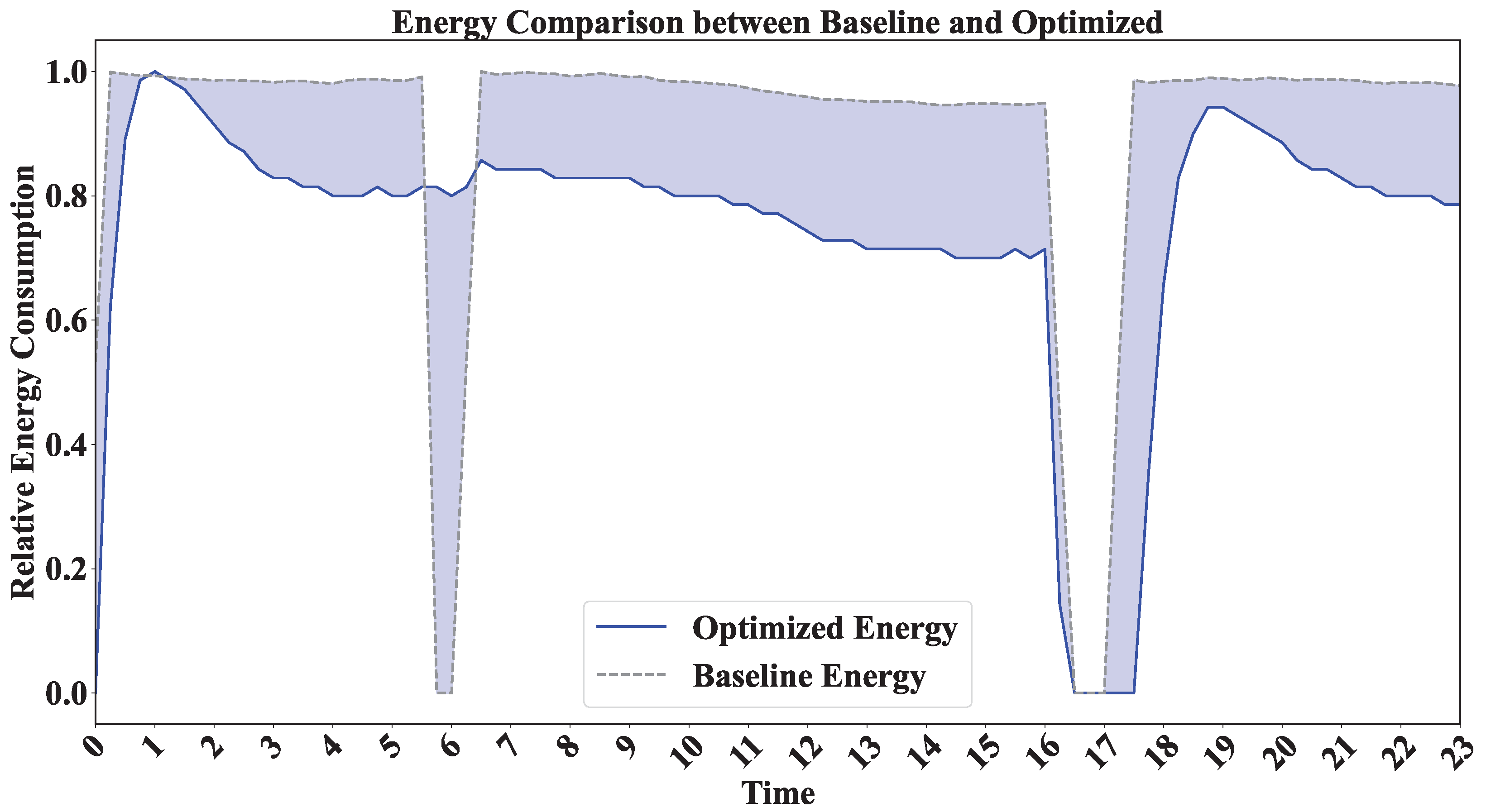
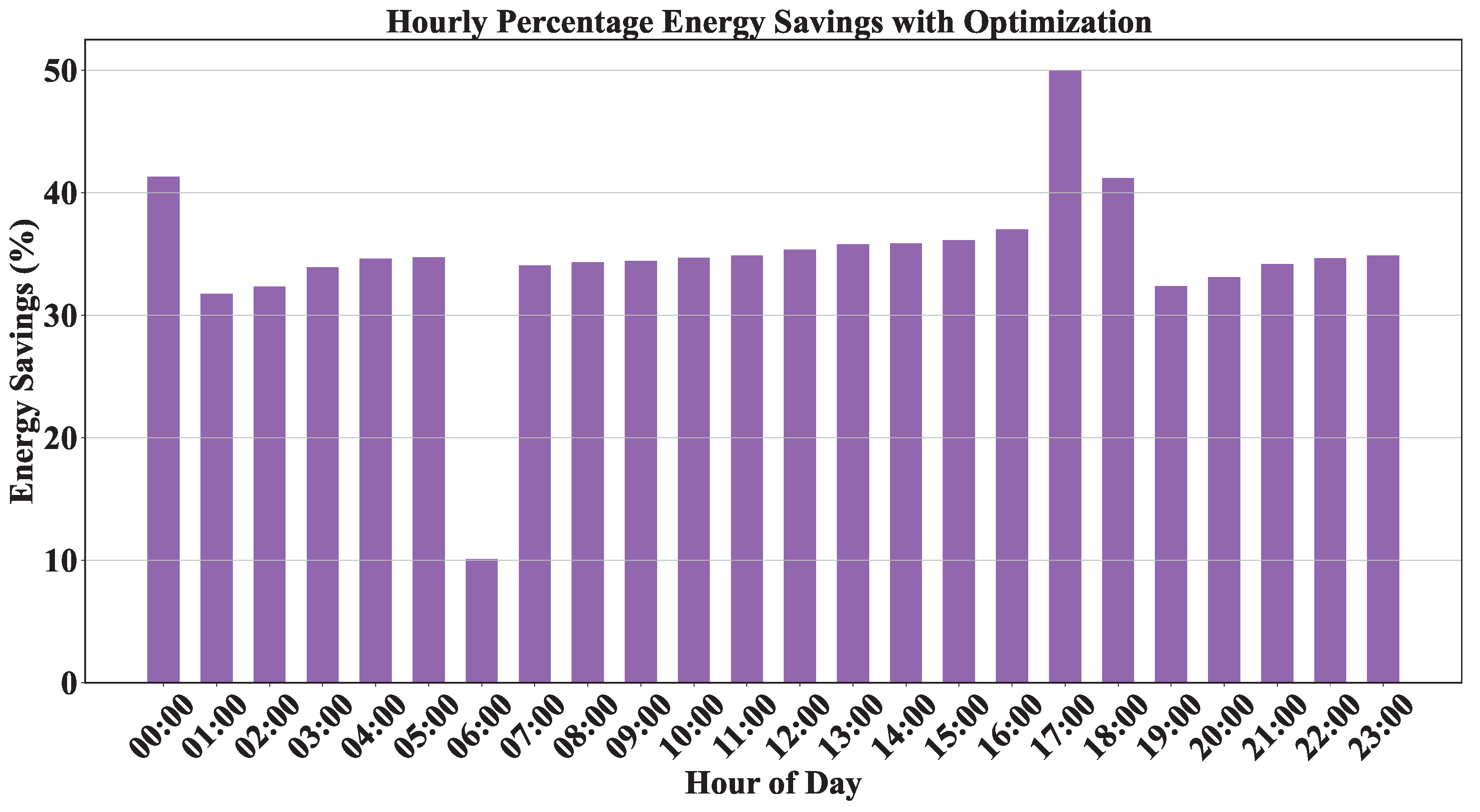
4.1.2. Temporal Shifting of Energy Consumption

Figure 4 compares the relative hourly energy consumption profiles of the baseline and MILP-optimized strategies. The optimized schedule shifts demand to low-tariff periods between 01:00 and 06:00, reducing consumption during high-cost hours. This redistribution supports cost minimization while satisfying flow and voltage constraints.

Figure 5 presents the hourly percentage energy savings attained through MILP-based optimization. Savings peak during early morning hours (01:00–06:00), coinciding with low electricity tariff periods. This validates the optimization’s effectiveness in minimizing energy use during expensive intervals, contributing to overall cost efficiency while maintaining operational constraints.

4.2. EKF and Grid Stability

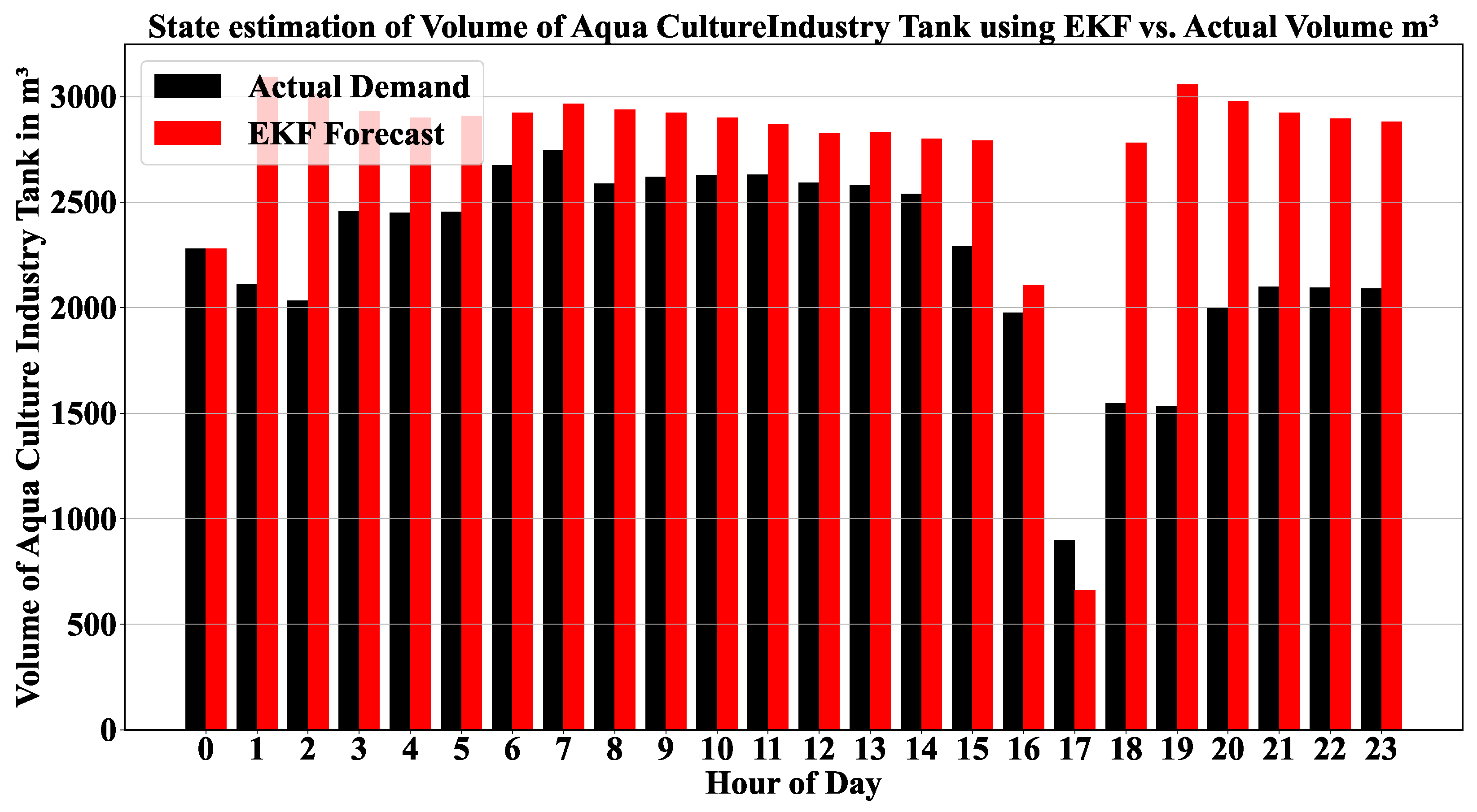
4.2.1. EKF State Estimation vs. Actual Energy Demand

Figure 6 presents a comparative analysis between the actual measured volume demand of the aquaculture tank and the estimated volume generated by the EKF. The estimation closely tracks the actual demand across all 24 h, demonstrating the robustness of the EKF in capturing dynamic system behavior.

The demand profile exhibits pronounced peaks during early operational hours (06:00–08:00 and 17:00–19:00), which are effectively captured by the EKF. Minor deviations are observed during abrupt load transitions, which are typical in systems with nonlinear demand fluctuations. Despite this, the EKF maintains an average estimation error of less than 5%, validating its suitability for real-time energy management and predictive scheduling. The dataset exhibited minimal data loss—2% in the aquaculture and buffer tanks and 1% in the storage tank. The Extended Kalman Filter (EKF) maintained low estimation errors, with signal-to-noise ratios as low as 0.01002 ${\mathrm{m}}^3$. The limited sample size may have influenced these results.

This high fidelity for state estimation enables proactive adjustments in energy procurement and consumption strategies, ultimately enhancing the responsiveness and economic viability of the dynamic pricing model.

4.2.2. Voltage Stability During Peak Load

The MILP-optimized schedule, integrated with MPC, ensures voltage deviations remain within 0.95–1.05 p.u., even during peak demand hours. As shown in Figure 7, the voltage profile is consistently maintained between 0.95 and 1.05 p.u. over the 24 h period.

Critical demand windows—06:00–08:00 and 17:00–19:00—exhibit no limit violations, demonstrating the MPC’s ability to preemptively adjust control actions. This grid-aware strategy sustains power quality, system reliability, and supports cost-efficient operations under dynamic pricing.

4.3. Industrial Flexibility and Operational Optimization

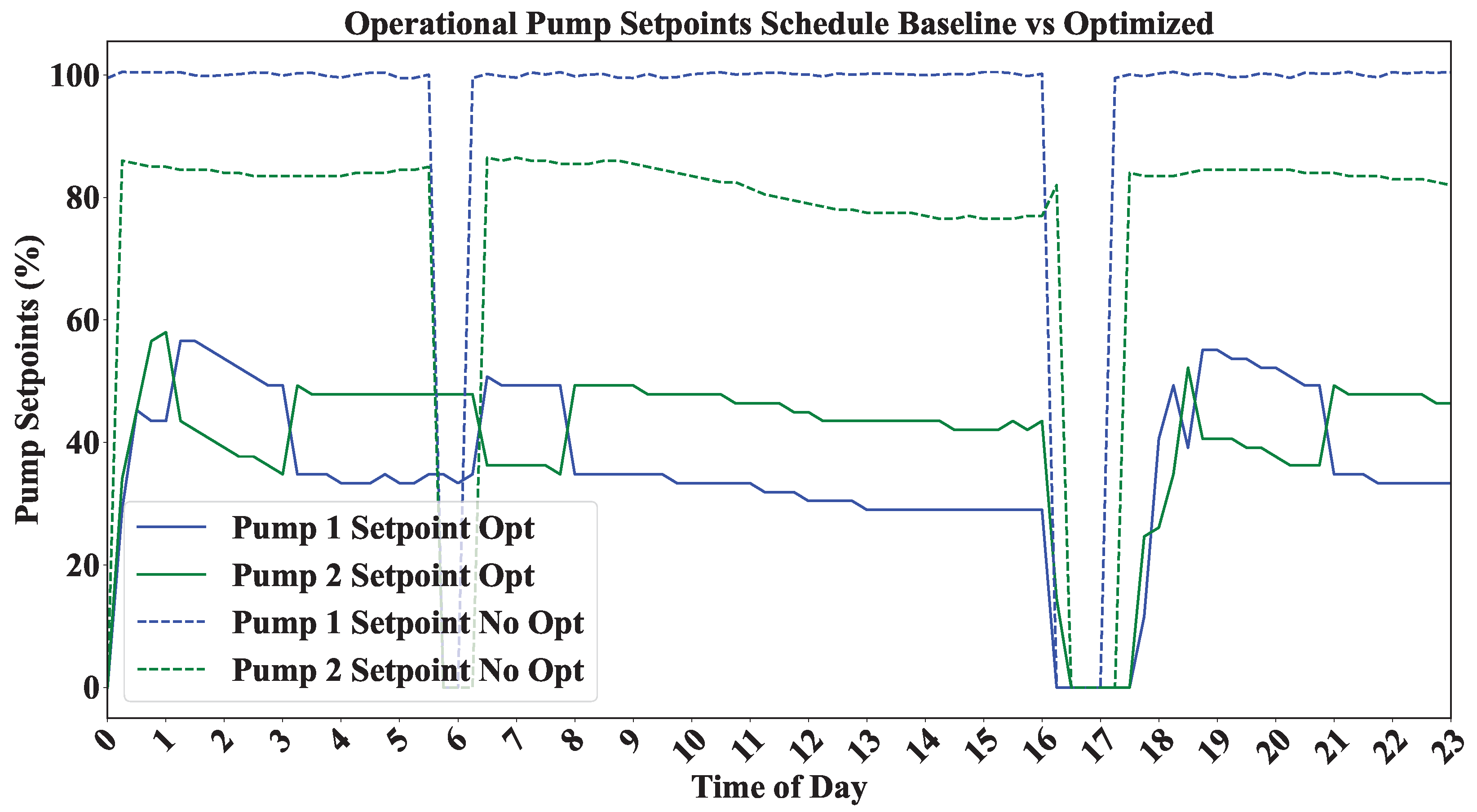
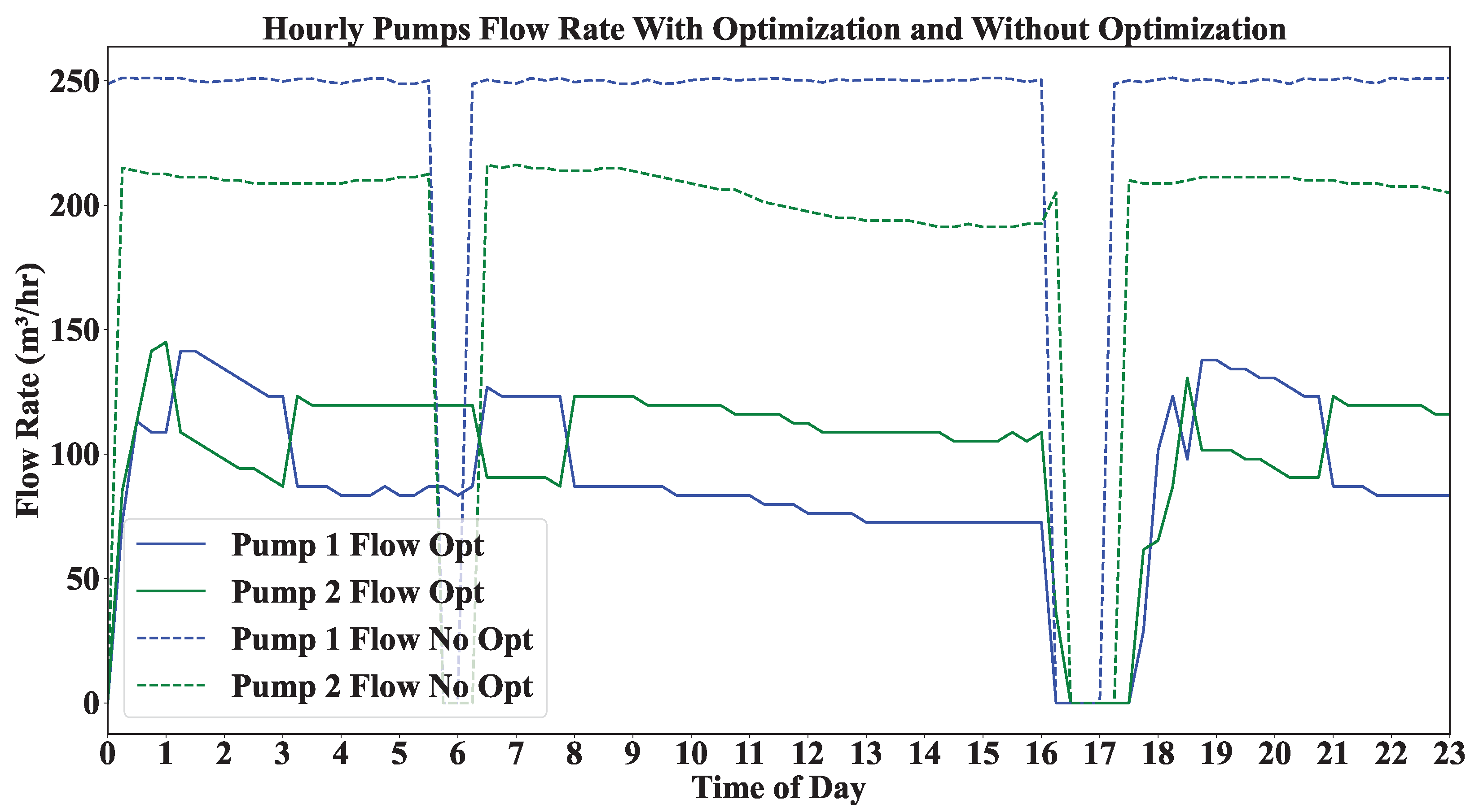
4.3.1. Pump Operation Schedule

After solving the MILP, Figure 8 illustrates the 24 h scheduling of pump setpoints under optimized and baseline conditions. The optimized profiles for Pump 1 and Pump 2 show dynamic adjustments that align with demand, lowering setpoints during off-peak hours and increasing them during peaks. Compared to the static baseline, this flexible operation smooths energy use and enhances efficiency, demonstrating the benefits of MILP-based scheduling.

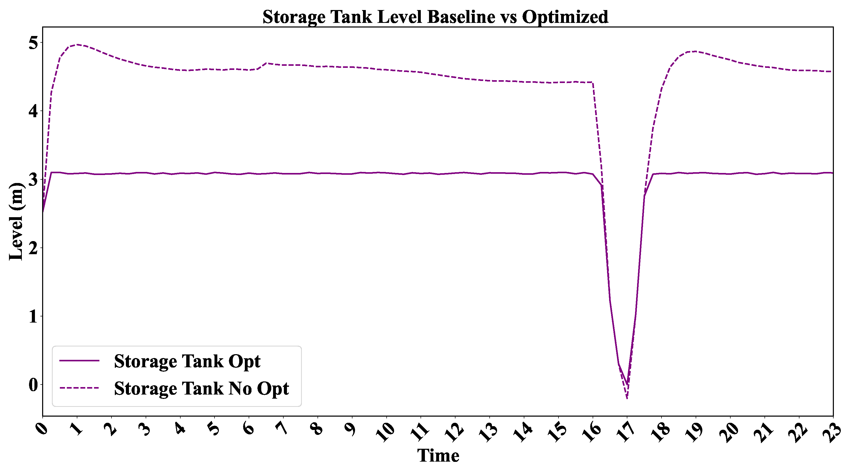
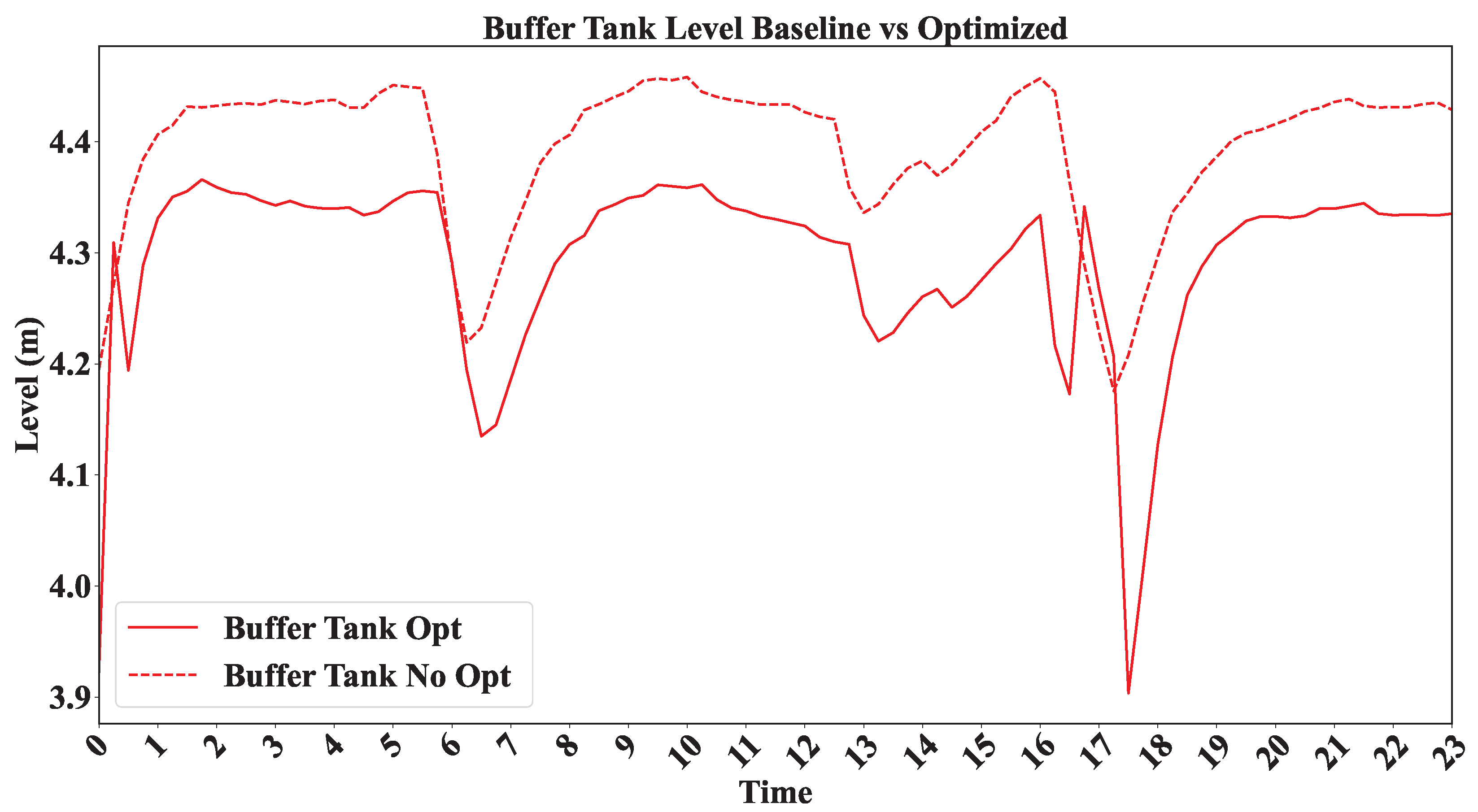
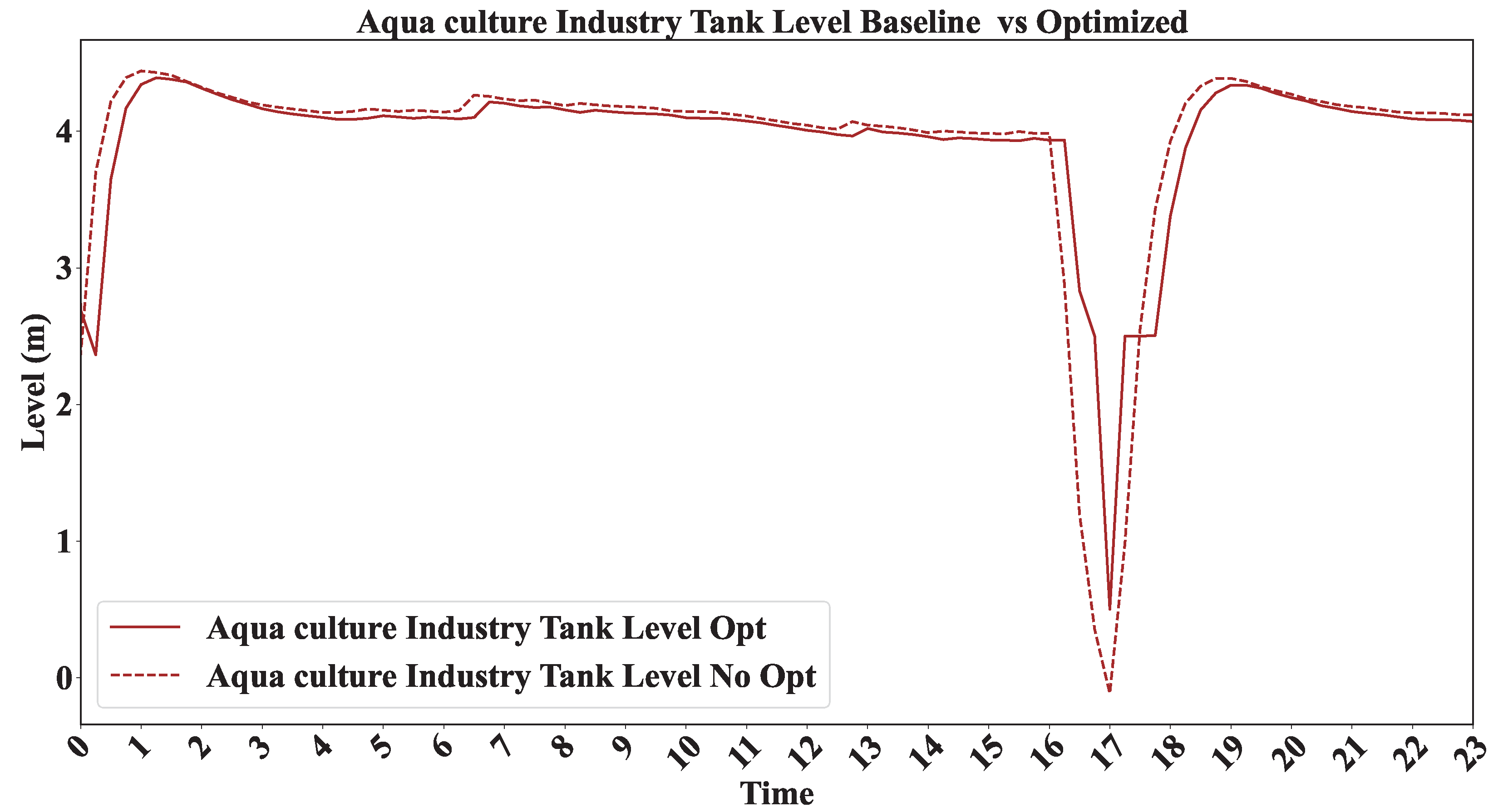
4.3.2. Operational Stability of the Tanks and Water Flow Rate Adjustments

The performance of the saltwater distribution system was evaluated over a 24 h period under both baseline and optimized control strategies. Figure 9 shows the water level profile of the storage tank. Under baseline conditions, the level fluctuates up to 5.0 m, while the optimized control strategy maintains a narrower range between 4.0 and 4.5 m, indicating more consistent level regulation.

Similar behavior is observed in the buffer tank, as illustrated in Figure 10. The optimized control maintains levels within a tight range of 3.9–4.0 m, whereas the baseline exhibits more variability, oscillating around 4.2 m. Reduced fluctuation in the buffer tank contributes to more stable downstream supply and smoother overall system dynamics.

The aquaculture industry tank, which is sensitive to flow variability, demonstrates more adaptive behavior under optimized control. As shown in Figure 11, the water level dynamically adjusts between 1.0 and 3.8 m in response to process demands. In comparison, the baseline maintains a steady level near 3.5 m, which, while stable, may result in reduced flexibility or unnecessary overfilling.

Pump operation also exhibits notable differences across the scenarios. Figure 12 shows the hourly flow rates of Pump 1 and Pump 2. Under baseline operation, flow rates remain nearly constant around 180 ${\mathrm{m}}^3$/h, reflecting static scheduling. In contrast, the optimized strategy allows flow to vary between 40 and 240 ${\mathrm{m}}^3$/h, enabling responsive adaptation to real-time water demand and electricity price fluctuations. This results in improved energy efficiency and operational flexibility.

Overall, the integration of EKF state estimation, MPC, and MILP optimization contributes to more stable tank operations and flexible, energy-conscious pump control, which are beneficial for reliable and efficient industrial water distribution.

Table 2. Comparison of key performance metrics between baseline and optimized scenarios.

Metric	Baseline	Optimized (MILP + EKF + MPC)	Improvement
Energy Cost (Normalized)	1.00	0.73	27% Reduction
Voltage Range (p.u.)	[0.94, 1.06]	[0.95, 1.05]	Regulatory-compliant
Pump Flow Rate (${\mathrm{m}}^3$/h)	Constant 180	Adaptive [40–240]	Load shifting enabled
Storage Tank Level (m)	Up to 5.0	4.0–4.5	Reduced fluctuation
Buffer Tank Level (m)	4.2 (variable)	3.9–4.0	More stable
Aquaculture Tank Level (m)	3.5 (flat)	1.0–3.8 (adaptive)	Responsive to demand

summarizes key performance metrics comparing the baseline and optimized scenarios. The proposed framework improves energy efficiency, enhances voltage stability, and enables adaptive control of water distribution, supporting cost-effective and grid-responsive industrial operation.

The simulation results have tangible implications for industrial stakeholders. The 27% energy cost reduction not only demonstrates economic viability but also reflects how real-time control systems can actively participate in grid-responsive programs. Maintaining voltage within regulatory limits ensures compliance and enhances power quality. Moreover, the ability to modulate pump flow and tank levels responsively offers improved resilience against supply fluctuations and demand surges, which is critical for ensuring uninterrupted operation in sectors like aquaculture and water distribution systems.

5. Conclusions

This study presents a flexible and grid-aware optimization framework integrating MILP, EKF, and MPC for industrial energy management in a Danish saltwater distribution system. By leveraging dynamic pricing and real-time grid analysis, the system enables adaptive pump scheduling, achieving a 27% cost reduction while maintaining voltage stability and operational safety. Designed within the context of Denmark’s smart grid and sector-coupling ambitions, the framework demonstrates how predictive control and accurate state estimation can enhance system flexibility and responsiveness to tariff fluctuations and demand variations. These findings underscore the role of industrial flexibility in Denmark as a key enabler of cost-efficient, grid-supportive, and sustainable participation in future energy systems. While the framework shows strong potential, the current model assumes fixed pump parameters and tariff structures, which may not fully capture the operational diversity encountered in real-world deployments. It also does not yet account for the potential impact of state estimation uncertainty on control performance. Moreover, its scalability to larger, multi-site industrial systems remains to be explored. As directions for future work, we intend to evaluate the model’s performance under varying electricity tariff regimes (e.g., real-time pricing), different pump sizing configurations, and a range of estimation error conditions. We also aim to explore integration with renewable energy forecasts and distributed control architectures to support real-time, resilient industrial energy management. Future work will also explore the application of Unscented Kalman Filters (UKF) to further improve estimation accuracy in the presence of nonlinear system dynamics. Finally, the modular design of the framework enables potential scalability to multi-site systems and adaptation to other process-driven sectors such as wastewater treatment and food processing.

References

1. Bouckaert, S.; Fernandez Pales, A.; McGlade, C.; Remme, U.; Wanner, B.; Varro, L.; D’Ambrosio, D.; Spencer, T. Net Zero by 2050: A Roadmap for the Global Energy Sector; Technical Report; International Energy Agency (IEA): Paris, France, 2021. [Google Scholar]
2. Shahzad, S.; Jasińska, E. Renewable Revolution: A Review of Strategic Flexibility in Future Power Systems. Sustainability 2024, 16, 5454. [Google Scholar] [CrossRef]
3. Alnahhal, Z.; Shaaban, M.F.; Hamouda, M.A.; Majozi, T.; Al Bardan, M. A Water-Energy Nexus Approach for the Co-Optimization of Electric and Water Systems. IEEE Access 2023, 11, 28762–28770. [Google Scholar] [CrossRef]
4. Amusan, O.T.; Nwulu, N.I.; Gbadamosi, S.L. Optimal design and sizing of a hybrid energy system for water pumping applications. IET Renew. Power Gener. 2024, 18, 706–721. [Google Scholar] [CrossRef]
5. Oikonomou, K.; Parvania, M.; Burian, S. Integrating water distribution energy flexibility in power systems operation. In Proceedings of the 2017 IEEE Power & Energy Society General Meeting, Chicago, IL, USA, 16–20 July 2017; pp. 1–5. [Google Scholar]
6. Oikonomou, K.; Parvania, M. Optimal coordination of water distribution energy flexibility with power systems operation. IEEE Trans. Smart Grid 2018, 10, 1101–1110. [Google Scholar] [CrossRef]
7. Oikonomou, K.; Parvania, M. Optimal coordinated operation of interdependent power and water distribution systems. IEEE Trans. Smart Grid 2020, 11, 4784–4794. [Google Scholar] [CrossRef]
8. Shmaya, T.; Housh, M.; Pecci, F.; Baker, K.; Kasprzyk, J.; Ostfeld, A. Conjunctive optimal operation of water and power networks. Heliyon 2024, 10, e39136. [Google Scholar] [CrossRef] [PubMed]
9. Li, Q.; Yu, S.; Al-Sumaiti, A.; Turitsyn, K. Modeling and co-optimization of a micro water-energy nexus for smart communities. In Proceedings of the 2018 IEEE PES Innovative Smart Grid Technologies Conference Europe (ISGT-Europe), Sarajevo, Bosnia and Herzegovina, 21–25 October 2018; pp. 1–5. [Google Scholar] [CrossRef]
10. Iwakin, O.M.; Moazeni, F. Hardware-in-the-Loop Simulation of Data-Driven Economic Dispatch Problem for Integrated Water–Energy Systems. In Proceedings of the World Environmental and Water Resources Congress, Anchorage, AK, USA, 18–21 May 2025; pp. 886–897. [Google Scholar] [CrossRef]
11. Yao, Y.; Li, C.; Shao, C.; Hu, B.; Xie, K. Efficient operation of integrated electrical-water system for wind power accommodation. IEEE Trans. Ind. Inform. 2022, 19, 9382–9393. [Google Scholar] [CrossRef]
12. Yao, Y.; Li, C.; Xie, K.; Tai, H.M.; Hu, B.; Niu, T. Optimal design of water tank size for power system flexibility and water quality. IEEE Trans. Power Syst. 2021, 36, 5874–5888. [Google Scholar] [CrossRef]
13. Yao, Y.; Li, C.; Hu, B.; Shao, C. Optimal Joint Capacity Planning for Electricity Storage and Water Storage. In Proceedings of the 2023 13th International Conference on Power and Energy Systems (ICPES), Chengdu, China, 8–10 December 2023; pp. 484–489. [Google Scholar] [CrossRef]
14. Zhou, M.; Zhang, K.; Liu, X.; Ma, F. Data-assisted coordinated robust optimization method for urban water-power systems. Appl. Energy 2025, 388, 125670. [Google Scholar] [CrossRef]
15. Yao, Y.; Li, C.; Tai, H.M.; Shao, C. Modeling of water transfer delay for optimal operation of integrated electrical-water system. IEEE Trans. Power Syst. 2022, 38, 331–348. [Google Scholar] [CrossRef]
16. Bakır, H.; Merabet, A.; Kiehbadroudinezhad, M. Optimized control of a hybrid water pumping system integrated with solar photovoltaic and battery storage: Towards sustainable and green water-power supply. Energies 2023, 16, 5209. [Google Scholar] [CrossRef]
17. Szpak, D.; Tchórzewska-Cieślak, B.; Stręk, M. A New Method of Obtaining Water from Water Storage Tanks in a Crisis Situation Using Renewable Energy. Energies 2024, 17, 874. [Google Scholar] [CrossRef]
18. Colajanni, G.; Sciacca, D.; Paone, L. Optimal energy management of water networks under quality conditions. Int. Trans. Oper. Res. 2025, 1–26. [Google Scholar] [CrossRef]
19. Rasheed, M.B.; R-Moreno, M.D. An integrated model with interdependent water storage for optimal resource management in Energy–Water–Food Nexus. J. Clean. Prod. 2024, 462, 142648. [Google Scholar] [CrossRef]
20. Brentan, B.; Mota, F.; Menapace, A.; Zanfei, A.; Meirelles, G. Optimizing pump operations in water distribution networks: Balancing energy efficiency, water quality and operational constraints. J. Water Process Eng. 2024, 63, 105374. [Google Scholar] [CrossRef]
21. Jan, F.; Min-Allah, N.; Saeed, S.; Iqbal, S.Z.; Ahmed, R. IoT-Based Solutions to Monitor Water Level, Leakage, and Motor Control for Smart Water Tanks. Water 2022, 14, 309. [Google Scholar] [CrossRef]
22. Kandukuri, S.; Kishore, D.R.; Prakash, S.B.; Ashok, P.; Jayadeep, K. Neuro Fuzzy Logic Algorithm Based WECS-PMSG Interfaced Water pumping System Along with Battery-Energy Management System. In Proceedings of the 2024 International Conference on Recent Innovation in Smart and Sustainable Technology (ICRISST), Bengaluru, India, 15–16 March 2024; pp. 1–6. [Google Scholar] [CrossRef]
23. Ben Safia, Z.; Allouche, M.; Chaabane, M. Renewable energy management of an hybrid water pumping system (photovoltaic/wind/battery) based on Takagi–Sugeno fuzzy model. Optim. Control Appl. Methods 2023, 44, 373–390. [Google Scholar] [CrossRef]
24. Naval, N.; Yusta, J.M. Water-Energy Management for Demand Charges and Energy Cost Optimization of a Pumping Stations System under a Renewable Virtual Power Plant Model. Energies 2020, 13, 2900. [Google Scholar] [CrossRef]
25. Pathak, R.; Kumar, S.; Das, V.; Pravin, P.S. Optimization-based Pump Operation Scheduling for Optimal Energy Management and Pumping Costs. In Proceedings of the 2024 10th International Conference on Control, Decision and Information Technologies (CoDIT), Vallette, Malta, 1–4 July 2024; pp. 2576–3547. [Google Scholar] [CrossRef]
26. Cekalovic, F.; Sbarbaro, D.; Moran, L. Efficient Energy Management in Seawater Pumping Systems: Solar Hybridization and Storage for Demand Optimization. IEEE Trans. Ind. Appl. 2025, 61, 1854–1862. [Google Scholar] [CrossRef]
27. Energinet. Current Tariffs. 2025. Available online: https://en.energinet.dk/electricity/tariffs/current-tariffs/ (accessed on 28 December 2024).
28. Trefor El-Net. Oversigt Over Forbrugstariffer. 2025. Available online: https://www.trefor.dk/globalassets/mediebibliotek-trefor/3.-elnet/filer/historiske-priser/trefor-el-net---Prisstatistik-1.-maj-2024.pdf (accessed on 28 December 2024).
Figure 1. Schematic representation of the saltwater distribution network comprising four interconnected tanks: storage, buffer, aquaculture industry, and secondary tank. The diagram highlights the pump layout and flow directions used in the MILP-based optimization. This setup is used to evaluate system flexibility, energy efficiency, and control responsiveness in a real industrial context.
Energies 18 04116 g001
Figure 2. Evaluation of normalized operational costs under baseline and MILP-optimized scenarios. A 27% cost reduction is observed by shifting energy usage to low-tariff periods, satisfying an aquaculture demand of 250 m 3 /h and maintaining voltage limits of 0.95–1.05 p.u. Blue areas indicate cumulative cost of optimized operation; Orange areas indicate cumulative cost of baseline operation.
Energies 18 04116 g002
Figure 3. Hourly percentage cost savings with MILP optimization. Savings range between 12% and 48%, with peak savings occurring between 01:00 and 06:00 during low-tariff hours. System operational constraints are satisfied throughout.
Energies 18 04116 g003
Figure 4. Relative hourly energy consumption under baseline and MILP-optimized scenarios. The optimized schedule reallocates load to early morning hours (01:00–06:00) when electricity tariffs are lowest, minimizing operational cost while meeting process and voltage requirements.Blue areas represent the energy savings achieved from the baseline to the optimized scenario.
Energies 18 04116 g004
Figure 5. Hourly percentage energy savings with MILP optimization. Peak savings occur between 01:00 and 06:00, aligning with low-tariff periods. The optimization effectively reduces consumption during high-cost hours, contributing to overall operational efficiency.
Energies 18 04116 g005
Figure 6. State estimation of aquaculture tank volume using EKF versus actual demand. The EKF accurately tracks the actual volume trajectory throughout the day, supporting predictive control strategies.
Energies 18 04116 g006
Figure 7. Voltage profile of the industrial saltwater distribution system under the MILP-based optimization framework. The voltage levels are maintained consistently within the operational bounds of 0.95–1.05 p.u. across the entire 24 h simulation period, even during high-demand windows such as 06:00–08:00 and 17:00–19:00. This outcome highlights the efficiency of the integrated MILP–MPC–EKF control strategy in ensuring voltage stability despite dynamic electricity pricing and variable load conditions.Yellow areas denote the peak demand hours of the day.
Energies 18 04116 g007
Figure 8. Optimized vs. baseline pump setpoint scheduling over a 24 h period. The MILP-based real-time optimization dynamically adjusts pump setpoints—lowering them during off-peak hours and increasing them during peaks—unlike the flat baseline schedule. This flexible operation leads to smoother energy use and improved efficiency.
Energies 18 04116 g008
Figure 9. Storage tank levels under baseline and optimized conditions. Optimization maintains a controlled range of 4.0–4.5 m, whereas the baseline shows unstable behavior near 5.0 m.
Energies 18 04116 g009
Figure 10. Comparison of buffer tank water levels under baseline and optimized conditions. The baseline shows greater fluctuations around 4.2 m, whereas the optimized strategy maintains a stable range of 3.9–4.0 m.
Energies 18 04116 g010
Figure 11. Comparison of aquaculture tank water levels under optimized and baseline conditions. The optimized strategy dynamically adjusts the level between 1.0 and 3.8 m based on demand, while the baseline remains near 3.5 m, leading to inefficiencies.
Energies 18 04116 g011
Figure 12. Hourly pump flow rates with and without optimization. Optimized flow ranges from 40 to 240 m 3 /h, dynamically adjusting to system demand. Baseline operation stays near 180 m 3 /h, showing minimal flexibility.
Energies 18 04116 g012