Article

Pre- and Post-Self-Renovation Variations in Indoor Temperature: Methodological Pipeline and Cloud Monitoring Results in Two Small Residential Buildings

Department of Architecture and Design, Politecnico di Torino, 10125 Turin, Italy
*
Author to whom correspondence should be addressed.
Energies 2025, 18(15), 3928; https://doi.org/10.3390/en18153928
Submission received: 20 June 2025 / Revised: 17 July 2025 / Accepted: 18 July 2025 / Published: 23 July 2025

Abstract

The impacts of renovation actions on pre- and post-retrofitting building performances are complex to analyse, particularly small and potentially self-actuated actions, such as adding insulation layers to a cold roof slab or changing doors. These interventions are widespread in small residential houses and cases where the owners are the residents. However, a large research gap currently remains regarding the impact of sustainable solutions on building performance. This study aims to address this issue by proposing a methodology based on commercial cloud monitoring solutions and middleware development that analyses and reports on the impact of such solutions to end users, allowing for an analysis of real variations in air temperature levels. The methodology is applied to two single/double-family residential houses, acting as demo cases for verification, across a multi-year time horizon. In both cases, measurements were conducted before and after typical limited renovation actions. Alongside the proposed methodology, descriptions of the smart solutions’ requirements are provided. The results mainly focus on temperature variations. Finally, the impact of the solutions on energy consumption was analysed for one of the buildings, and feedback was briefly provided by the users.

1. Introduction

During recent decades, several countries and the European Union (EU) have shown much interest in defining and supporting actions and regulations aimed at reducing the energy and climate impact of buildings, with the latter being responsible for more than 40% of the total primary energy needs and more than one third of the Green House Gas emissions in the EU [1,2]. The mentioned actions mainly help to define minimal energy requirements for new and existing buildings under renovation—see, for example, ref. [3]—and define incentivising policies.
At the European level, the renovation market is expected to grow from USD 956.88 billion in 2021 to about USD 1012.47 billion in 2026 [4]. Hence, the topic of building stock renovation has become essential—at least in a context such as the European one, where current policies incentivise this type of intervention to reduce energy consumption and improve the indoor environmental quality (IEQ) of confined spaces. Among other policies, the Green Deal initiatives [5], the Next Generation EU [6], and the Renovation Wave EU [7,8] are worth mentioning. Additionally, national incentives and economic bonuses have been introduced to support end users in making significant renovations to buildings in the hope of improving their buildings’ Energy Performance Certification (EPC) classification. Moreover, in specific contexts—such as in Italy—some categories of small retrofitting actions qualify, for example, for tax payback of part of the costs.
Nevertheless, building renovation is a vast and complex topic, requiring not only the support and incentivisation of actions but also verification of the real impact of those renovation actions to avoid performance gaps (PGs) between the expected individual and political performances and the ones currently achieved during building operation [9,10].
Post-intervention evaluations are complex to perform, especially if they include IEQ analyses, due to the lack of available data before and after the renovation [11,12,13]. The possibility of communicating the impact of a retrofitting action to the end users is also limited, as these types of analyses are generally used for research purposes or were developed by energy management companies of large buildings, such as ESCOs, to minimise the rebound effect of PGs in the first years after the intervention to maximise their payback [14,15]. Moreover, these mentioned challenges become almost impossible to address when the analysed action is not an extensive renovation but a specific intervention managed by a small building owner to a focused area, such as window or door substitutions or the addition of an insulation layer to the floor of a cold storage attic.
This study aims to address the above-mentioned research gaps, focusing on the latter, which is very diffuse in contexts where the resident is also the owner; for example, in European Member States such as Italy. The proposed methodology, developed during an EU-co-founded H2020 project—called the Next Generation of Energy Performance Assessment and Certification [16]—adopts smart monitoring systems and data elaboration platforms to support multiple analyses, including real-time suggestions and performance gap detections via digital twins; see [17,18,19]. Given this background, this study focuses on developing and applying an additional functionality of intelligent monitoring solutions: verifying the impact of renovation actions. Using measured data analyses, the approach can overcome the pre- and rebound effects of PGs [20,21,22]. This work extends part of the mentioned project H2020 studies and complements their outcomes [23].

1.1. Literature Review

Post-renovation studies are mainly based on simulation campaigns or a limited number of field measurements, generally used to validate models, due to the complexity and costs of installing sensors and leaving them active in lived environments. This aspect increases the risk of PGs—see, for example, refs. [9,20,22,24,25]—particularly to the rebound effect of PGs, i.e., where the expected results are higher than those obtained.
Several studies have highlighted how theoretical models and their correlated useful tools often fail to capture the full complexity of real-world building behaviours and occupant actions [26]. Specifically, the authors of [27,28] have emphasised the importance of intensively monitoring internal conditions, physical building characteristics, and occupant behaviours to obtain a more accurate and realistic evaluation of a building’s energy performance. In such studies, data collected during monitoring are used to calibrate simulation models, improving energy consumption predictions and thermal comfort following retrofit interventions.
The importance of such monitoring becomes even more evident when considering that thermal comfort and indoor air quality are strongly influenced by occupant behaviour. Studies such as [29,30] have shown that user behaviour, such as temperature management or ventilation systems, can significantly impact energy outcomes and occupant well-being. In particular, Ref. [30] studied occupant behaviour in relation to heating and ventilation systems, demonstrating that everyday habits can substantially reduce the effectiveness of retrofit interventions, especially when individual thermal sensitivity and preferences are not considered. This study supports the idea that continuous monitoring can improve the management of internal comfort and optimise the energy performance of buildings, identifying a specific research gap that needs to be studied and analysed in future studies.
Similarly, Ref. [31] combined field measurements before and after renovation interventions on a Swedish residential complex with building energy modelling techniques. The authors identified two lateral outcomes in their work: i. part of the expected energy saving resulted in an increase in indoor temperatures, raising the winter IEQ, and ii. assumptions of the simulation input may strongly impact the expected post-intervention performances, as they are not aligned with real user behaviours, underlining an open challenge. Other studies tried to address this latter challenge by including occupancy behavioural surveys [29,32] or analysing manual operation of smart solutions correlated with IEQ and energy conditions [33]. Nevertheless, a detachment between users and performances is still evident, not providing end users with consistent results regarding the impact of their retrofitting actions on their building performance (both energy and IEQ), especially in the long run. The importance of considering residents’ IEQ perceptions in post-renovation analyses is also underlined in specific studies, such as [29,34]. Ref. [34] underlines the correlation between the possibility of receiving positive residents’ feedback and their level of information and building perceived control. Hence, developing new studies about post-renovation intervention analyses and restitution performance is essential for residents to increase their information and involvement.
Ref. [21] demonstrated how integrating advanced technologies for monitoring air quality and internal conditions can significantly increase the energy efficiency of buildings and minimise energy performance gaps. This work uses real-time sensors to measure environmental conditions and occupant response. The importance of developing new integrated middleware platforms, which are capable of integrating real-time measured data and simulating building behaviours, has also been underlined in other recent works, such as [17], where a new dynamic platform was developed and tested in demo cases, identifying almost real-time building PGs and communicating them to end users for counteractions. The effectiveness of adopting smart solutions to cover the building energy PG was also analysed in other studies, such as verifying the impact of standard variations in input on energy and IEQ indicators [13,35]. Nevertheless, additional work on functional integration needs to be developed to discuss how intelligent monitoring systems can be adopted in additional building performance subtopics, such as post-intervention analyses.
The importance of low-energy automated energy system management is a recurring theme in retrofit studies, such as those in [36] on residential retrofitting in Athens, and in [37] in the UK. The results suggest that tailoring interventions based on specific building characteristics and environmental conditions is crucial. Thus, combining predictive simulations and empirical data is essential for effectively calibrating interventions and correctly identifying pre-intervention challenges and post-intervention performances [38]. Nevertheless, the authors recognise that climate and occupant behaviours are critical determinants in retrofitting solution success. Data acquisition and analysis are essential challenges to correctly analysing post-intervention impacts [39].
These studies support the idea that an intelligent building management system can significantly improve energy performance and indoor environmental quality. Nevertheless, this type of solution opens up the possibility of additional applications that have not yet been explored, such as the possibility of analysing post-renovation interventions affordably and feasibly, with special regard to small retrofitting actions. This study aims to cover these challenges.
Additionally, all the above-mentioned studies have focused on significant building renovation actions, considering mainly multi-storey residential buildings subjected to deep retrofitting interventions and never small, limited and, in several cases, self-performed renovations, such as those that do not require construction permission or local administrative authorisation, being generally referred to as independent retrofitting actions. The latter are very diffused, especially in countries where the building property is very segmented and the residents are generally also the owners, such as Italy. In such cases, including single-family houses, but also flats, single window or door substitutions, the addition of insulation in specific under-roof or semi-buried garage ceiling segments, as well as changes to the heating system, constitute typical interventions are not considered during pre- and post-intervention analyses. These changes can cause some positive variation in EPC. However, the latter generally results in performance gaps [9,17,24]. Although the impact of these interventions can be analysed by end users, who also designed and performed them, based on differences in costs or personal sensation, such as IEQ, the possibility of examining this impact in higher detail and providing scientific performance feedback remain urgent research gaps, which this study aims to cover.

1.2. Study Objectives

This study aims to achieve the following:
  • Introduce and demonstrate an affordable and reproducible method for assessing post-intervention building performance by using intelligent building monitoring and management platforms to return results to the end users;
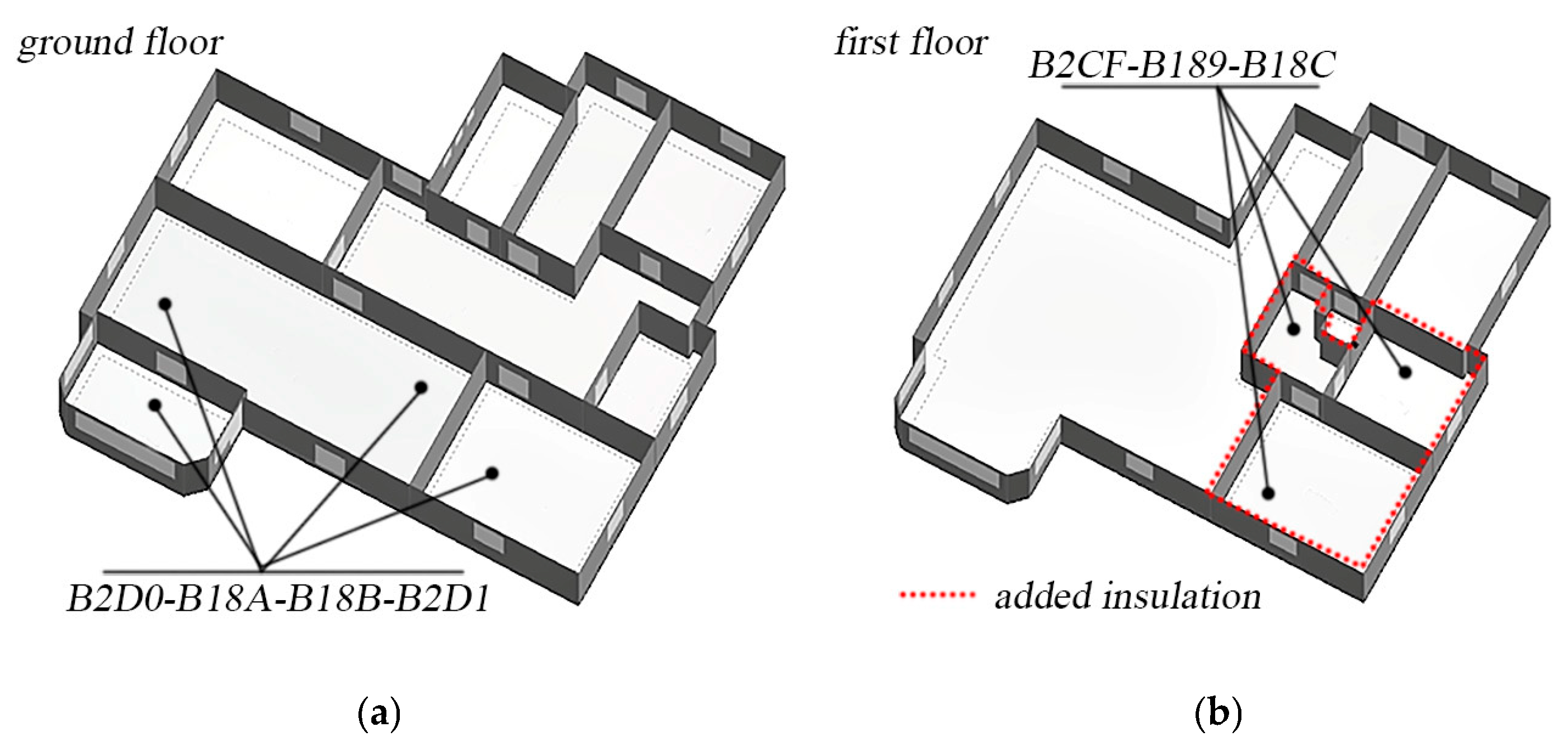
  • Conduct post-renovation analyses to study the impact of small typical interventions such as door substitutions or the addition of simple insulation layers, e.g., on the extrados of the last slabs under the unoccupied roof or on the ceiling of a garage located below the living spaces, that are very representative of what arrives in individual houses or in flats of multi-family houses where the residents are also the owners.
To pursue these objectives, the cases of two residential demo buildings were assessed to verify the potential usage of intelligent monitoring solutions and middleware platforms in analysing the impact of small retrofitting interventions, exploiting data elaboration potentialities. These two buildings are single-family residential houses, representing the Italian building stock of medium-to-small cities but aligned with most southern and mid-European contexts. This study analyses the retrofitting impact on the air temperature, considering small interventions. The choice of temperature variations was made because single-family houses generally do not use room-based thermostats or radiator thermostatic valves and these types of small interventions mainly impact IEQ profiles.

1.3. Novelties

Section 1.1 underlines the need to conduct additional studies to develop and test new methodologies and correlated monitoring solutions, paying special attention to techniques that may find applications for a larger audience and can be adopted for small retrofitting interventions. The impact of these small renovation interventions is not a deeply studied topic, resulting in a research gap in current works on post-renovation analyses, which this study aims to overcome. The first research question this study seeks to answer is as follows:
  • Q1: Is it possible to propose a simple and easily replicable methodology to study the impact of small and punctual retrofitting interventions, including self-renovation ones, that mainly affect IEQ and air temperature conditions?
Answering this research question is thus objective 2 of this study.
Additionally, several previous works have underlined how personal behaviours and building control logics may strongly differ from standard profiles, causing significant PGs in post-renovation analyses, especially when the use of in situ measurements is minimal. These gaps make providing feedback about the impact of the obtained interventions on the end users difficult, reducing the feasibility of the interventions and end user confidence. Nevertheless, the recent progressive diffusion of smart monitoring facilities suggests that this challenge may be overcome by exploiting their untapped potential. Studies are needed to propose and demonstrate methodologies and applications on this point. In addition, the few existing studies have mainly focused on energy savings in significant interventions, while small interventions generally affect more temperature profiles, increasing thermal comfort and varying IEQ. This study also aims to cover these gaps, proposing a newly developed methodology, a monitoring protocol, and a data-management middleware approach to support post-renovation air temperature analyses. The proposed method is compatible with additional features, such as the definition of optimal retrofitting scenarios via massive simulations and digital twins [40], aiming to integrate a larger set of functionalities into smart building middleware facilities [23]. These latter challenges result in additional research questions:
  • Q2: Is it possible to integrate pre- and post-retrofitting impact analyses within newly developed smart middleware monitoring solutions to exploit the untapped potential of those technologies in covering multi-applicational outcomes under long-term continuous monitoring actions?
  • Q3: Can these tools inform and support non-expert and expert end users during building operational management and small renovation interventions, reducing the lack of commitment and providing affordable feedback to occupants about their recent self-retrofitting actions and/or behavioural choices?
These two last questions make up objective 1 of the study.
This study makes the following contributions:
  • Focuses on small retrofitting actions that are generally never analysed in ex-post studies of building renovation due to the small correlation between invested budget and complexity, but which are very typical and diffused in the majority of houses and flats when the residents are the owners (or when the latter owns not the whole building but only a single flat);
  • Disseminates the results to users—ones directly defined and, in several cases, directly supported by the renovation actions—connecting retrofitting with direct IEQ variations;
  • Uses monitoring data before and after the intervention, and not during only one of the two phases;
  • Adopts commercial cloud-based intelligent monitoring solutions to analyse energy, especially IEQ parameters, allowing for the potential integration of this approach with newly diffusing middleware facilities;
  • Focuses on IEQ aspects—i.e., temperature—in parallel to energy savings in small houses where thermal variations among rooms may be consistent.

2. Materials and Methods

To address the study objectives and research questions, a monitoring solution which is compatible with many additional smart building features was established (see Section 3.1), and a data analysis methodology was developed (see Section 3.2). The monitoring system and the methodological pipeline were applied to two demo buildings, part of the Italian demo cases of the EU H2020 co-funded project E-DYCE (see Section 2.3). The selected case studies are two typical single- and double-family buildings which are representative of the building compounds of mid- to small-sized municipalities in Italy. Both are located in Torre Pellice, a municipality in northwest Italy, in the Val Pellice territory. Additionally, the site—which is part of the Turin metropolitan area—is highly representative of typical residential areas in north and central Italy, in terms of building typology, municipality dimension, and climate characteristics (Italian Climate Zone F, 3128 Heating Degree Days [41], and Cfb Koppen–Geiger climate type—temperate oceanic climate [42,43]). These demo buildings experienced small retrofitting interventions during the measurement periods, allowing for an investigation into the effect of self-placed thermal insulation additions to roofs and basements, door substitutions, and heating system improvements. The following sections detail the developed methodology to analyse the pre- and post-retrofitting impacts, focusing on IEQ performance rather than the energy requirements.

2.1. Setting the Monitoring Infrastructure

An intelligent monitoring system was selected and installed at the demo sites. The monitoring system was created based on the following technical and functional requirements:
  • Allows for high replicability of the solution, adopting a commercial sensor system and balancing the cost/benefit ratio;
  • Has a scalable and modular architecture;
  • Allows for remote access to data and sensors;
  • Supports multi-year cloud and local data storage capacity;
  • Reduces data loss by adopting preventive solutions, such as redundant storage and avoidance of data loss during potential connection failures;
  • Minimises the need for fixed energy plugs (i.e., based on batteries) to reduce installation costs and to allow for higher acceptability by occupants;
  • Includes high-security data access protection protocols;
  • Uses gateway connections independent from local Wi-Fi networks, e.g., using independent SIM solutions (facultative).
The modular Capetti Electronics Winecap commercial system, Castiglione Torinese ITA [44] was selected as it uses dataloggers with different internal or external probe configurations, supporting scalability and modularity. All loggers support a battery plug, while the sole gateway modules require an electrical plug connection. Each component—i.e., the dataloggers and gateways—has the capacity for local storage, overcoming potential connection challenges and preserving the monitoring functionalities from data losses. The system can support failures to connect to the local gateway, allowing for data storage at the logger level until the specific sensor is again accessible to the gateway. It also supports internet connection issues, as the data are stored at the gateway level and automatically transmitted and stored in the cloud facility when the connection is re-established. The data are stored in a cloud and accessible via the Winecap web portal. Gateways are SIM-based, not requiring local networks. The cloud service can be accessed via the SOAP protocol [45] and via REST, which allows for strong security and high reliability. The system transmits data to the server every hour or less. Data collection at the probe level can be programmed to acquire data at smaller intervals, even remotely. For this study, the monitoring acquisition granularity was set to 10 min. Furthermore, outdoor conditions were measured via a meteorological station with REST API access. This facility was installed on a nearby roof and allowed for the generation of actual meteorological years supporting additional usages not described here—see, for example, [17]. The weather station was composed of a US climate sensor by Thiess [46] and a Delta Ohm pyranometer LP-PYRA-02 (1st class) [47].
For this study, the monitoring solution was set at the room level, measuring temperature and relative humidity in all spaces (probe type WSD00TH2_LD), including non-heated ones. In contrast, CO2 concentration levels were measured in the main rooms, including kitchen, living room, bedrooms, and studios (probe types WSD00TH2CO_S and WSD00TH2CO). Table 1 describes the instrument accuracies and measuring ranges. The sensors were positioned following the specifications given by the company, not directly exposed to solar radiation, while positioned at about 1.5 m from the ground, primarily on indoor walls in a central position. In both demo buildings, continuous measurements were taken for more than 2 years, between 2021 and 2023.

2.2. Analysis Method

During the project period, targeted renovations were carried out in the two residential buildings, part of an Italian project’s demo site. In both cases, the impact of these retrofit measures was analysed by elaborating on the data retrieved from the above-described monitoring infrastructure. For both buildings, indoor temperature profiles rather than energy consumption were examined. However, in the following Discussion section, the energy bills for the first demo site and the bioclimatic comfort charts of the second demo site were also studied. Air temperatures were analysed because in the first building the installation of the energy meters was coincident with the retrofit measure, for which no historical data are available, with the exclusion of bills while, in the second building, the thermostat facility is located far from the retrofitted rooms—in the lower floor—and the renovation was not performed to address the energy needs but for local thermal comfort during winter.
For the two buildings, the IEQ temperature-based study adopts the following analyses:
  • Carpet plot diagrams created with the newly developed PREDYCE tool [48,49], showing measured air temperatures throughout the whole multi-year period to evaluate whether visible changes occur pre- or post-renovation;
  • The statistical distribution of temperatures (average, standard deviation, and quartiles), focusing on the previous result;
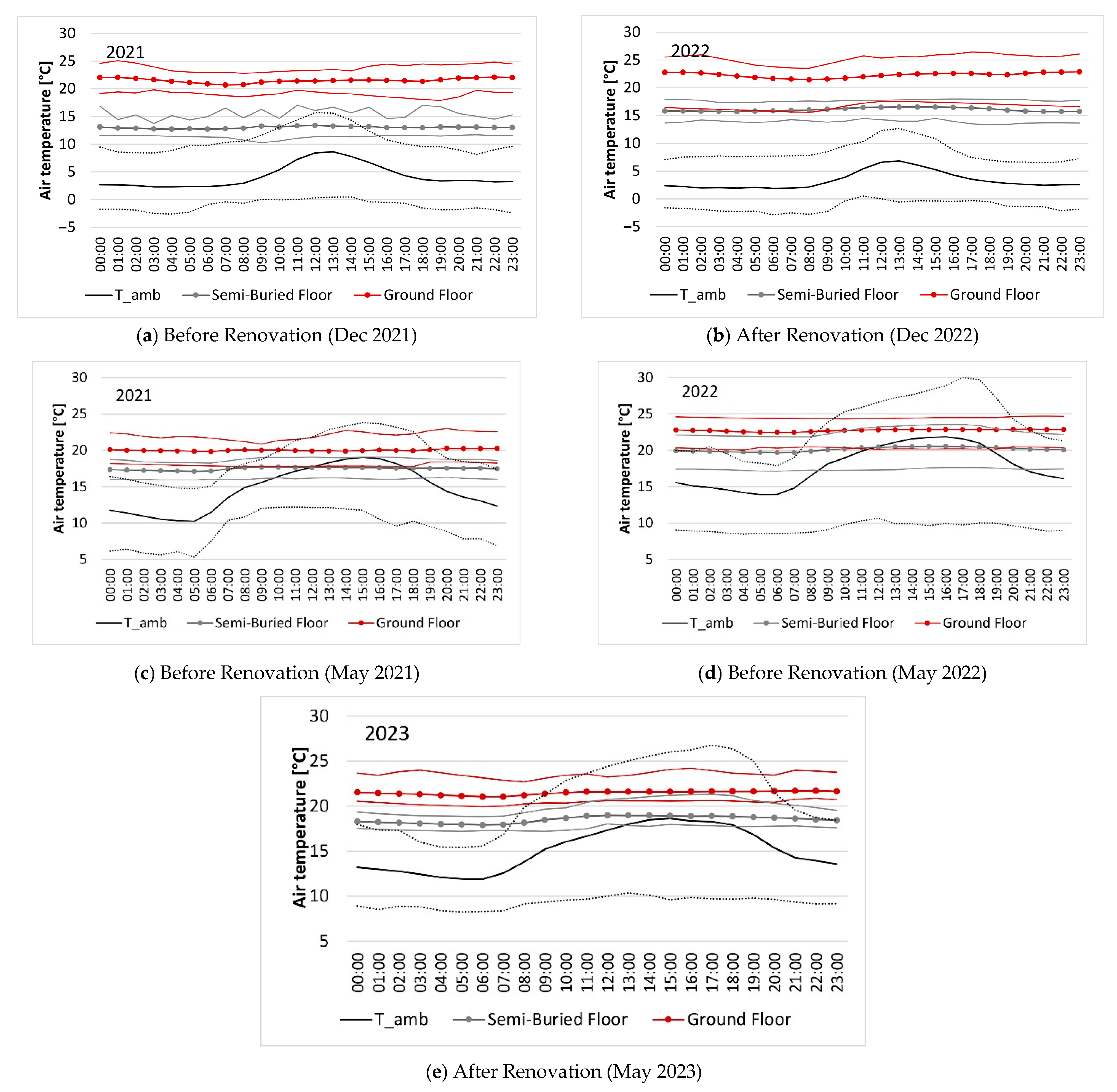
  • Temperature variations in representative seasonal months—i.e., December for winter and June for summer—comparing measured air temperatures during the air conditioning period (winter heating) and the non-air-conditioned period (summer free-running), respectively, before and after the measurements.
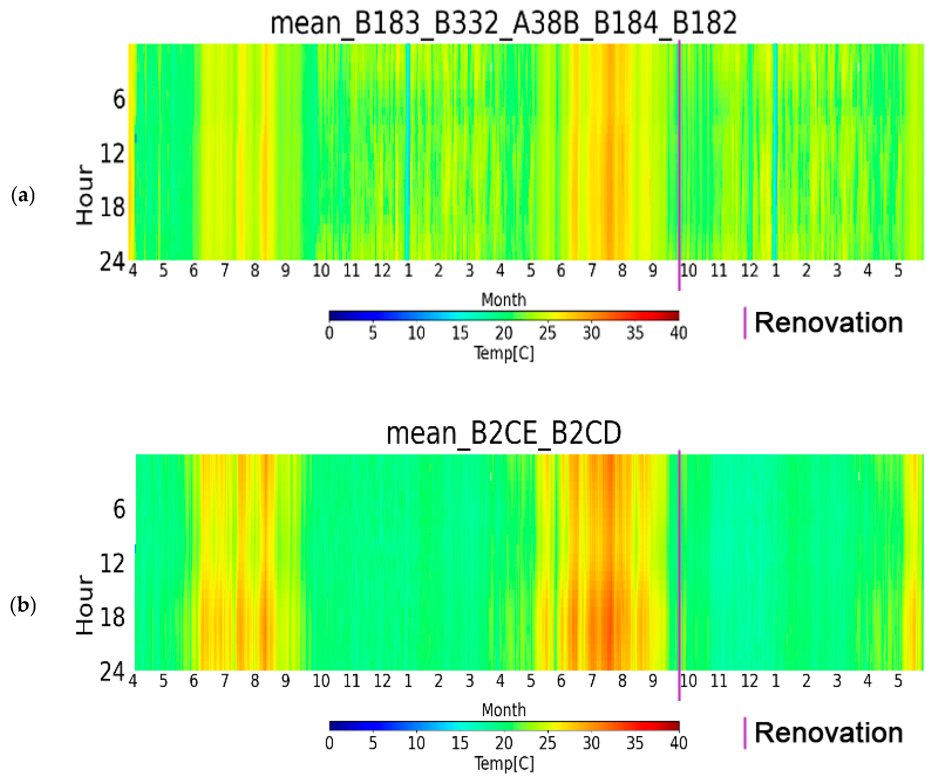
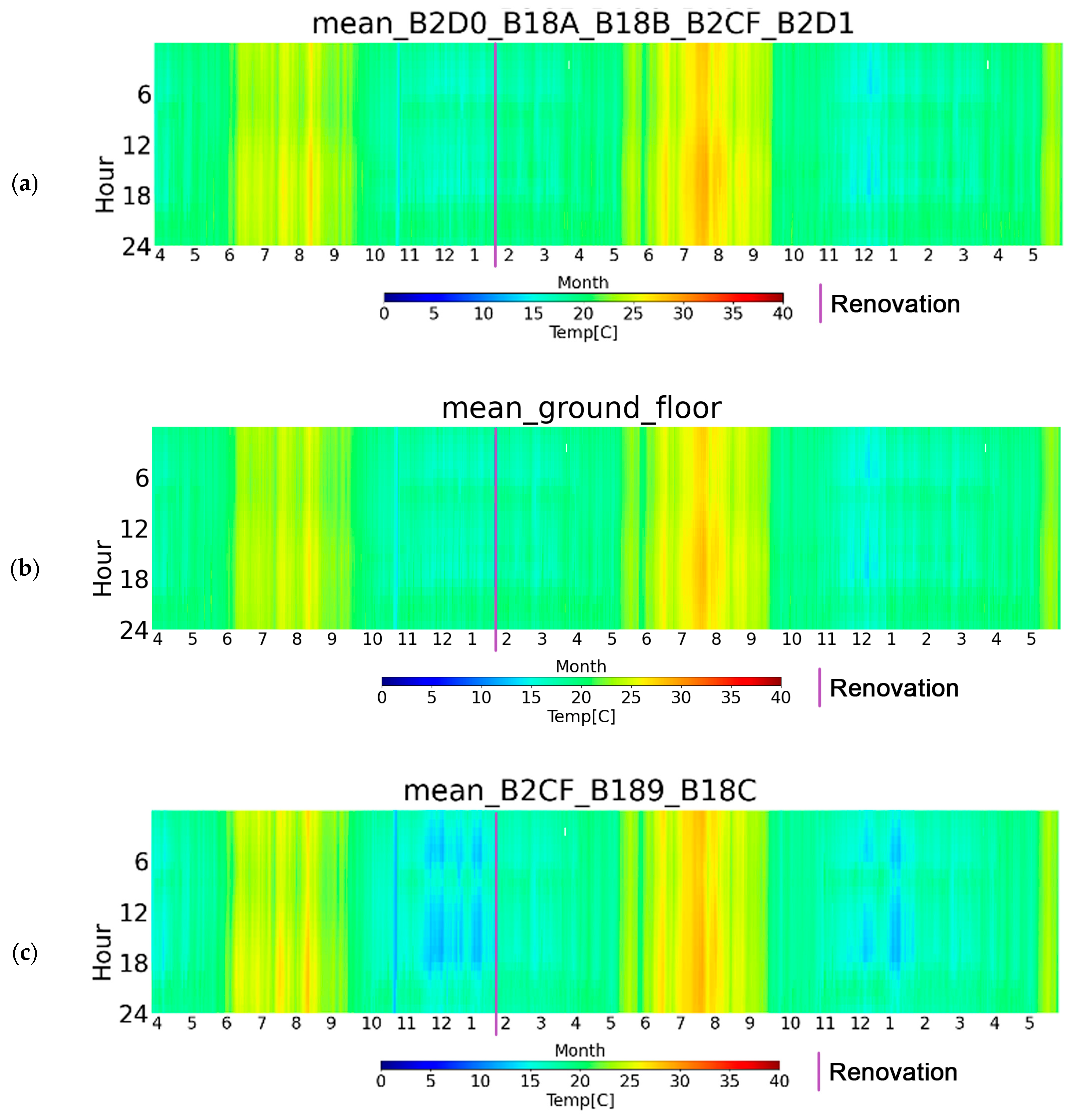
  • Twenty-four-hour average daily hourly profiles for representative seasonal months;
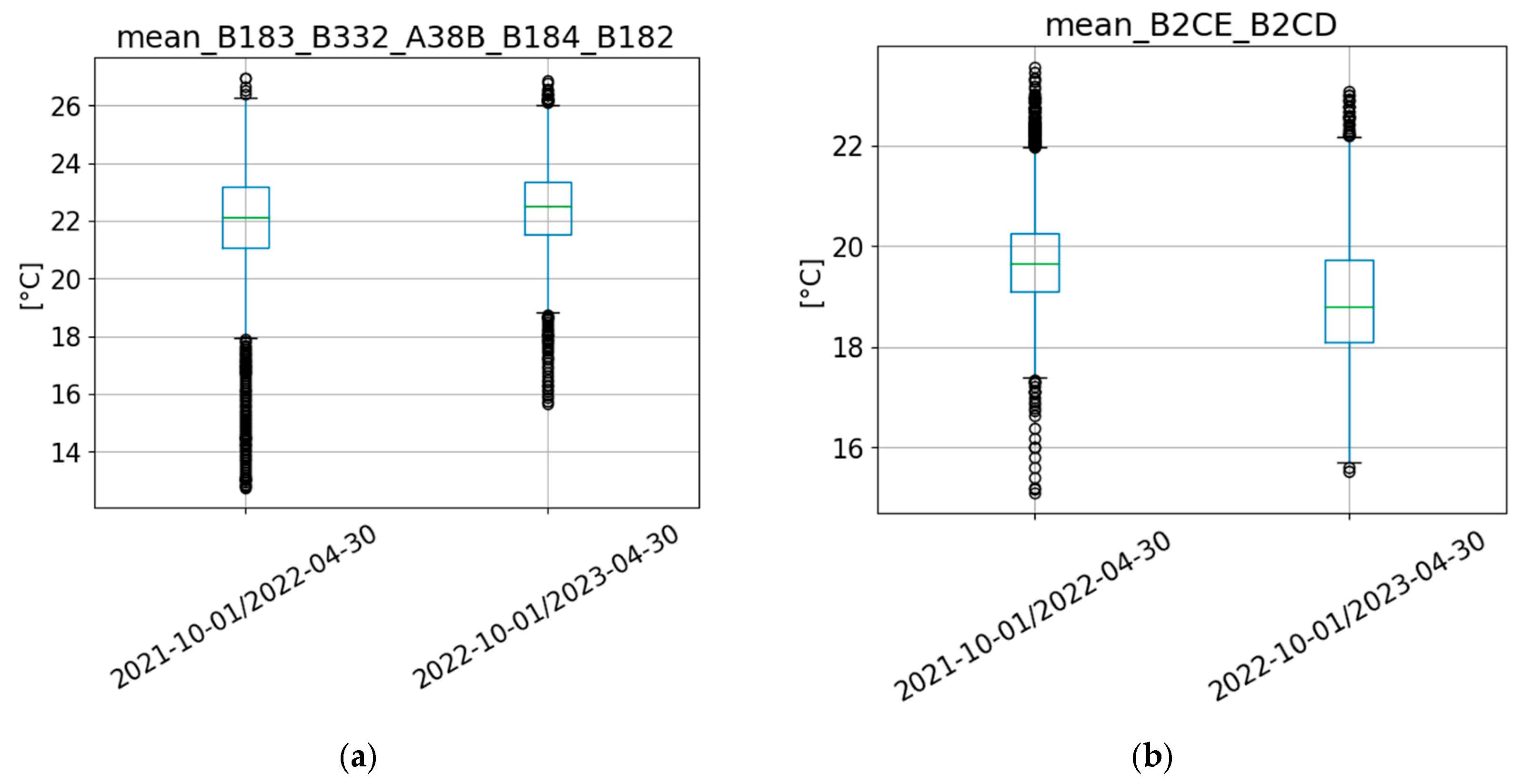
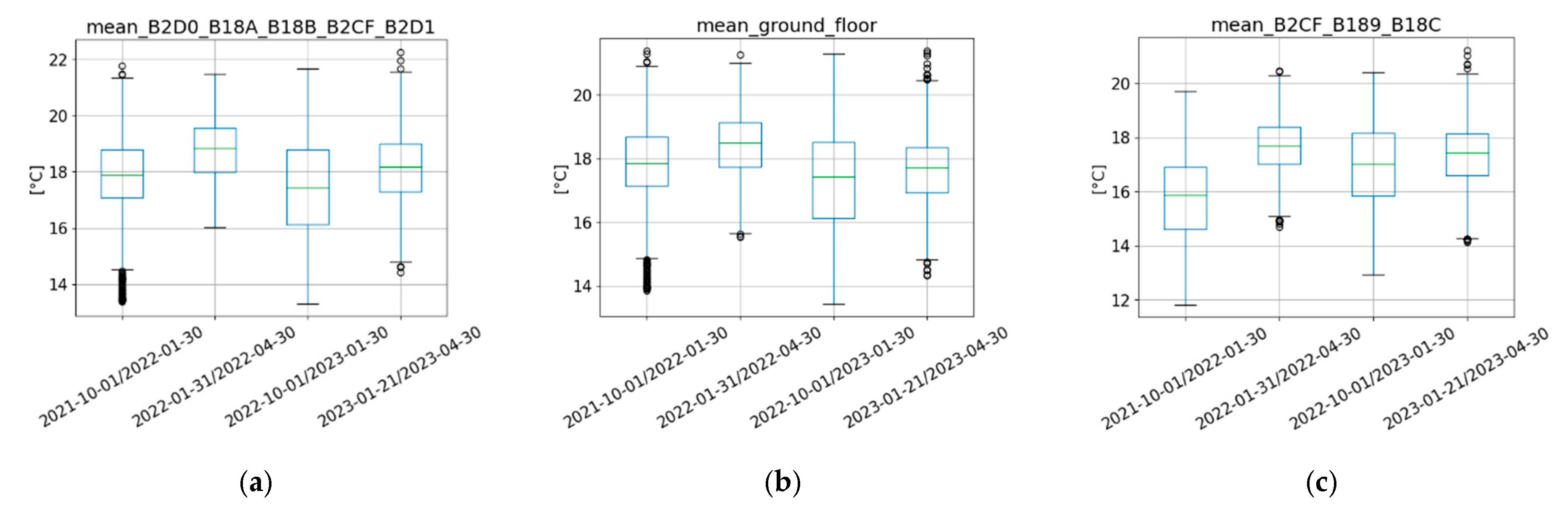
  • Box and whisker plots reporting statistical distributions of the measured temperatures for the extended heating season (October to April) before and after the renovation, which allow for a comparison of the minimum, first quartile, median (horizontal lines in the boxes), third quartile, and maximum values, plus the outliers as separated dots. Boxes connect the 25th% to the 75th% percentiles. The whiskers represent the first and fourth quarters.
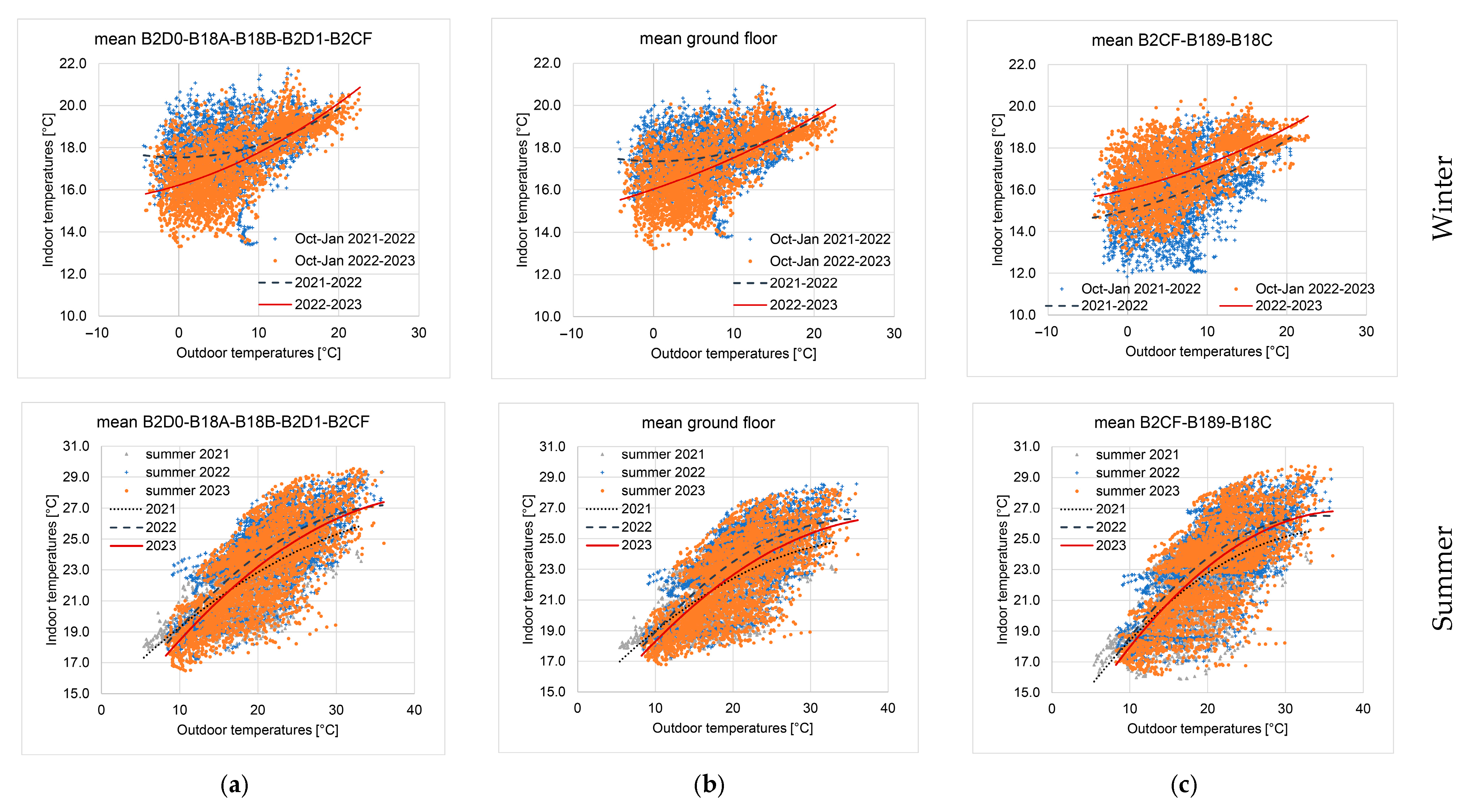
  • Scattered plots plotting indoor temperatures as a function of the outdoor ones to detect the impacts of renovation on indoor/outdoor correlations and to support a weather-independent discussion.
The discussion section also briefly comments on i. the impact of renovation actions on energy consumption for the first building (bill analysis), including heating degree day (HDD) normalisation, and ii. an extended IEQ thermal comfort analysis, including thermal comfort models for mechanically treated periods (winter), i.e., the Fanger PMV-PPD method, and for free-running periods (summer), i.e., the adaptive thermal comfort model, aligning with the current CEN standards. CO2 concentrations are not analysed as the specific retrofitting interventions do not directly act on relevant variations in airtightness, i.e., windows were not changed and ventilation systems were not present.

2.3. Case Study Description

2.3.1. Demo 1

This residential demo case is situated in a historic “Borgata,” a dwelling group typical of the Italian mountains, with origins before the 20th century. The building structure is based on stone and brick bearing walls with an irregular shape. The living room, kitchen, bedrooms, and bathroom are located on the main level, while the utility rooms are located in the semi-buried basement. The residents were a family with two young children who go to school during the morning, while one of the parents is often working at home. The structure had been renovated recently, changing from its original rural state to a state fit for residential use, and reaching an EPC of class E (2015). Nevertheless, during the period analysed here (2021–2023), this demo building experienced several minor typical renovation actions. Firstly, an insulation layer was added to the outermost layer of the ground floor, slab located between the non-climatised semi-buried basement and the conditioned main floor, between the end of September and the beginning of October 2022. Simultaneously, the heating facility was replaced with a new natural gas condenser heater coupled with a smart thermo-fireplace. The additional insulation layer was composed of polystyrene rigid panels: i. positioned 10 cm under the pavements of the bedroom, bathroom, and kitchen, facing the semi-buried unconditioned basement, and ii. installed 5 cm below the living room but facing the outside, as this space is supported by pilotis. Additionally, at the beginning of 2021, the doors leading towards the outside of the main floor were substituted with insulated ones with a U-value of 1 W/m2K. Figure 1 shows the analysed zones and the slabs where the insulation was added (red dashed lines). Pre- and post-renovation analyses were conducted on the average measured temperatures of the rooms on the main floor affected by the addition of insulation and the average of the two first-floor spaces.

2.3.2. Demo 2

This second residential building is in one of the urban expansion areas defined by the municipality’s 1914 zoning regulation. From a construction point of view, the building is composed of a reinforced concrete structural skeleton and brick curtain walls. It is a Liberty-style house built at the beginning of the 20th century as a detached double-family home surrounded by a private garden. It has two main floors, each with one apartment, an attic, and a cellar. It could be described as a typical Italian detached house built in the twentieth century with an EPC of class E (2018). The monitored areas were the ground floor and half of the first floor. Reference sensors were also positioned in the non-heated cellar and attic spaces (cold roof, not heated). The residents were a family with one child who goes to school in the morning, while the family spends their lunch break together at home.
The analysed renovation intervention was the self-installation of 14 cm (two overlapped layers of 7 cm each) of glass wool an insulation layer on the slab, positioned on the last slab’s outermost layer. This slab is the one between the first floor’s climatised and non-climatised spaces of the cold attic. The renovation was performed at the end of January 2022. At the same time, the small windows of the cellar were closed, affecting the temperature variations in the non-climatised buried floor. Before this renovation, these windows were left open. Figure 2 briefly identifies the monitored zones investigated in this study.

3. Results

3.1. Demo 1 Results

The carpet plots in Figure 3 show the variations in the measured air temperatures, in the main (a) and first (b) floors. The main renovations occurred at the end of September 2022—see the vertical lines in the charts. The data highlight that the temperatures in the ground floor are visibly higher for the post-renovation period during the 2022–2023 extended winter season (from October to April). A rise in temperatures also occurred on the upper floor in October 2022, while, for the following winter months, the temperatures were slightly lower post-renovation than before the retrofitting, even if they did not fall below 18 °C. After a discussion with the residents, it was confirmed that, after the renovation, the upper floor rarely required the radiators to run, as the thermostat consistently stayed above 18 °C. This explains why the temperatures on that floor did not show the same peaks. Additionally, the renovation also minimised the need to heat the upper floor, addressing the variations in the ground floor temperatures.
The seasonal statistical data from Table 2 synthesises the results. In winter, on the ground floor, the average temperature rises by 2% post-renovation (about +0.4 °C), while on the first floor, it decreases by −4% (−0.8 °C). From a general point of view, the renovation also impacted the relative humidity, which in both cases grows by +12% and +17%, respectively, on average (absolute increases of +4.1% and +7.1%). The results underline a general increase in the internal mixing ratios in alignment with that in the literature—e.g., [50]. In summer, temperatures increase by 4% on both floors (about +1 °C on average), while the relative humidity is more stable (a relative average growth of +4 and +5% for the ground and first floors). The average relative humidity in all seasons rises, but the measured values are within comfortable boundaries (see EN 16798-1 [51]), with a general average improvement in winter. Comparing the indoor values with the corresponding outdoor ones, the summer temperature increased even when the average outdoor temperature decreased (−8%). In contrast, the indoor winter humidity (mixed ratio) rose considerably more than the outdoor one, confirming the presence of these critical issues.
Figure 4 presents the representative monthly temperature variations. Looking at the winter period (December), the average ground floor temperatures align between the pre- and post-renovation periods, even if colder peaks, visible in the pre-renovation period, reduced after the retrofitting. Additionally, in the last period of the month, higher temperatures were recorded in the post-renovation period. These results highlight the intervention’s ability to activate thermal masses and reduce heat transmission via the newly insulated floor. Additionally, the semi-buried unconditioned spaces had higher temperatures than that during the pre-renovation year, even when the outdoor temperatures were lower, reducing the difference in temperature between the buffers and heated spaces. This reduction in difference is also due to the fact that the new heater was located in the basement. Differently, in the free-running season (May 2022 vs. May 2023), a decrease in temperatures is underlined in both the ground and semi-buried floors. However, 2022 was characterised by a long heat wave, proving to be an unconventionally hotter year. This was also confirmed in a comparison of the outdoor temperature lines in Figure 4b. For this reason, in Figure 5—which shows the 24 h average hourly profiles—the data related to May 2021 are also reported to allow for the unexpected summer behaviour to be verified. Figure 5, together with the previous Figure 3 and Table 2 data, shows that May 2023 was characterised by higher air temperatures in the confined spaces compared to those in 2021. These results underline that, as expected, the installation of consistent thermal insulation layers resulted in a post-renovation overheating risk in summer. Figure 6 confirms the above-mentioned winter outcomes. The box and whisker plots show an increase in the median and interquartile range (IQR) for the main floor, while the lower whisker minimum also rose after the renovation. Similarly, the described decrease in the first-floor data is also shown. However, the thermostat limit of 18 °C was maintained. The data extension of outliers was also drastically reduced for the first floor, showing a more stable temperature behaviour. Finally, the scattered graphs in Figure 7 report the indoor temperatures as a function of the outdoor temperatures. These analyses confirm the above discussions about seasonal variations, showing the described increase in the winter 2022–2023 temperatures on the main floor and their decrease in the first floor without statistically underpassing—see the polynomial regression line—the setpoint. The reported extended summer season trend (May–September) verifies the overheating risk due to the addition of the insulation layer, hidden by the heat wave 2022 in the results of Figure 4. Hence, the scattered plots compare the 2021 and 2022 data (pre-renovation) with those for 2023 (post-renovation). The results underline an overheating phenomenon post-renovation, visible for the rooms on the main floor for the entire external temperature interval. The main floor is, in fact, directly influenced by the addition of the thermal insulation layer. The first floor also experienced visible overheating after the retrofitting, especially when the outdoor temperatures exceeded 13 °C (the intercept of the 2021–2023 regressions was set at 12.73 °C). In particular, looking at the regressions, the difference in temperatures before and after the renovation was 0.8 °C on both the ground and first floors for an outdoor temperature of 20 °C and was almost maintained on the ground floor (0.7 °C at 25 °C and 30 °C) but rose on the first floor (1.1 °C at 25 °C and 1.4 °C at 30 °C) at higher outdoor temperatures.

3.2. Second Demo Results

Figure 8 shows the sub-hourly data carpet plots and the monthly statistical distribution of the measured temperatures for the second demo building. The plot shows the average measured data for the main rooms in the building, the average temperatures of the ground floor, and the average temperatures of the three zones on the first floor that are directly influenced by the additional insulation layer. The results firstly highlight an increase in the measured internal temperatures for summer 2022 compared to the same period during 2021. Secondly, concerning winter, a reduction in indoor temperature cold peaks is shown in October and November, especially on the first floor—see the reduction in small light blue hours during the mentioned period. Nevertheless, in late September and December, the indoor temperatures in 2022 were lower than those in 2021 for the whole building and the ground floor, but not for the first floor. After a discussion with the residents, it can be noticed that the thermostat was set lower in 2023 (19.3 °C) than in 2022 (19.8 °C). This discrepancy justifies the impact on the ground floor, where the thermostat is located. In contrast, the increase in air temperature on the first floor directly correlates with the renovation action by limiting the heat loss towards the roof. Table 3 focuses on seasonal averaged variations: in winter, temperatures decreased when comparing 2021–2022 with 2022–2023 on the ground floor (−3%, corresponding to −0.5 °C on average), although the first floor experienced an increase (+7%, corresponding to +1.1 °C); in summer, temperatures increased by 2% (+0.4 °C) and +3% (+0.6 °C) on average for the ground and first floors, respectively. From the relative humidity point of view, we also underline in this demo a growing trend with regard to the ground floor in winter (+17% relatively and +9.8% absolutely). Additionally, on the first floor, the relative humidity rose by +9% (absolute variation +6%), reaching an average value above 70%, suggesting that countermeasures must be adopted—see the categories for comfort in the EN 16798-1 standard [51]. In summer, relative humidity increased by 10–11% on both floors, rising to nearly 70%, suggesting that summer dehumidification occurred. The renovated conditions are hence more humid than expected, even when compared to outdoor values (a computed mixed ratio was used for comparing outdoor and indoor values in winter, with indoor temperatures rising from before to after retrofitting at +1 g/kg and +1.3 g/kg, respectively, for the ground and first floors, vs. +0.6 g/kg outdoors).
Figure 9 reports the representative monthly temperature behaviours for each season and shows an increase in temperatures in the post-retrofitting period, both in the unconditioned buffer spaces and the inhabited ones, especially in summer and on the first floor. The reported buffer spaces are for the ground floor, the cellar, the first floor, and the cold roof space. Regarding the first-floor behaviour, Figure 10 compares the average 24 h hourly profiles for December and June (2021 vs. 2022), underlining a more stable behaviour after the retrofitting in the lived spaces—in particular, in summer, the increase in attic temperatures was not correlated with a consistent rise in the temperature of the inhabited areas even when the weather was hotter. Inversely, the heated rooms behaved more stably even under colder weather in winter.
The above results were confirmed via the box and whisker plots of Figure 11. The first and third data series in the graphs were compared to analyse the impact of renovation actions on the measured building performances. In addition, the second and fourth series in the graphs, which both refer to post-renovation periods, are reported to study the impact of the above-mentioned reduction in set points. The latter analysis underlines how the ground floor temperatures have a colder median and IQR in 2023 compared to 2022. This confirms the discussed reduction in the set-point temperature. Focusing on the pre- and post-renovation comparison (Oct–Jan 2021–2022), the median on the ground floor also decreased. Still, this change is less evident than the previous one. However, the IQR increased after the renovation, resulting in higher temperature variations (potentially due to a change in the system activation schedule). Oppositely, considering the first floor, the graph highlights a different behaviour: the variations between the two post-renovation periods (Feb–April 2022–2023) were consistently regulated by the building (the thermostat is on a lower floor), while the temperatures of the first floor significantly rose post-renovation thanks to the positive effect of the addition of the thermal insulation layer on the under-roof slabs, reducing heat losses.
Figure 12 shows these variations as a function of the outdoor air temperatures to verify the above outcomes independently based on specific weather variations. In winter (from October to January), the regression lines confirm the previous results (see Figure 11): the ground floor is colder in 2022–2023; in contrast, the first floor is hotter, especially at lower outdoor temperatures. Similarly, a risk of overheating is confirmed for summer, recording higher temperatures for both floors in post-intervention periods (summer 2022 and 2023). The post-renovation increase in overheating phenomena mainly occurred at the hottest outdoor temperatures: The deltas between the 2021 and 2023 data are 0.2 °C and 0.4 °C at an outdoor temperature of 20 °C for the ground and first floors, respectively, but rise to 0.6 °C and 0.7 °C at 25 °C and to 0.9 °C and 1 °C at 30 °C.

4. Discussion

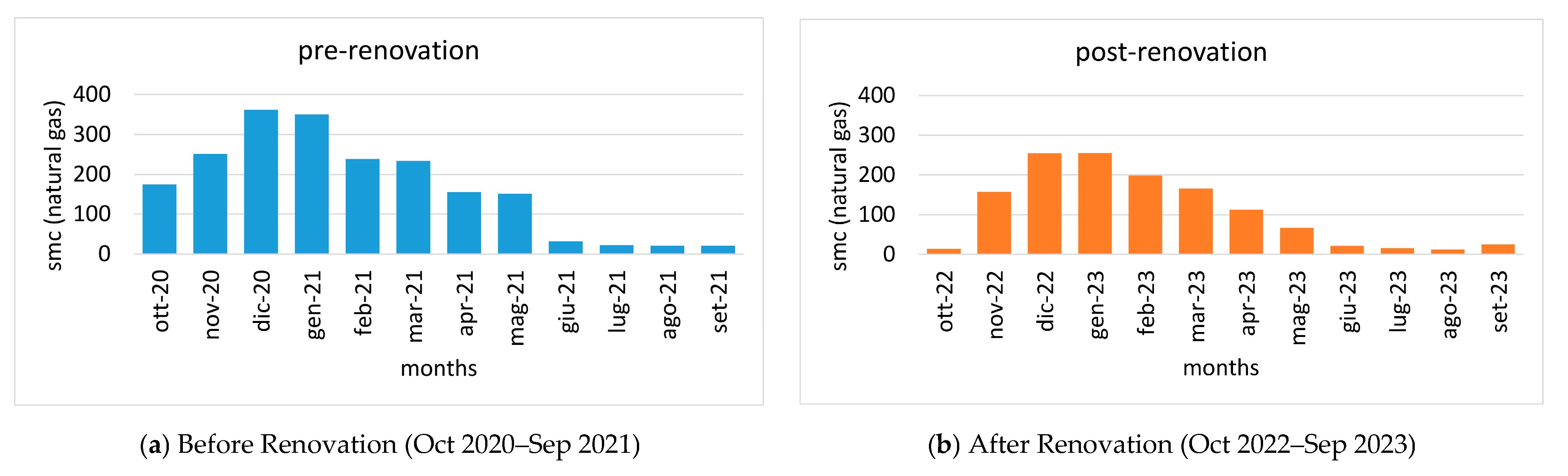
4.1. Impacts of Renovation on Energy Bills

In the Results section, the impacts of small typical renovation interventions were analysed based on the variations in air temperature. However, for the first demo site, due to the multiple renovation actions, the space also experienced a direct impact on energy consumption where the thermostats were located, including due to the substitution of the entire heating system with a new heater (natural gas condensation heating) coupled with a smart thermo-fireplace, which directly heated the living room and nearby areas, as well as supported the heating system since it also directly heated the radiator water distribution system. Nevertheless, since smart heat meters were installed after the renovation intervention, the pre- and post-renovation comparisons are performed based on the natural gas bills for this Discussion section. In line with the Italian EPC primary energy factors (PEfs) given by the UNI/TS 11300 standards [52,53], wood-based energy vectors correspond to a PEf of 0, so the thermo-fireplace is not considered here. The renovation did not directly impact the heating facility for the second demo. Still, it mainly affected the local temperature profiles of the first floor, while the thermostat was located on the ground floor. In this latter case, the heating system only relied on a pellet automatic heater; therefore, no bills are available. For these reasons, this section focuses on energy consumption variations in the natural gas bills before and after the self-renovation in demo 1. Figure 13 shows the natural gas smc units (standard cubic metre, equivalent of 10.60 kWh) consumed each month in the reference period, October 2020–September 2021, and in the post-renovation period, October 2022–September 2023. The graphs underline a large difference between before and after the renovations, decreasing from 2015 smc in 2020–2021 to about 1299 smc in 2022–2023. Although the values for 2021–2022 were influenced by the mentioned heat wave, with natural gas consumption reaching 1761 smc, in all cases, the post-retrofit energy consumption was considerably lower than the pre-retrofit energy consumption.
Figure 14 shows the data for the natural gas bill normalised according to the local measured heating degree days (HDDs) during the local standard heating season, ranging from October to April. Considering that the gas consumption data were collected progressively, the HDDs are based on the cumulative difference in temperature, weighting each measurement period for its time length. Outdoor temperature is measured based on the World Meteorological Organisation standards, i.e., data are collected every 5 min, and the time-weighted HDD is retrieved considering monthly cumulative values with a base temperature of 20 °C, aligning with the indoor set-point and the national standard base temperature [54,55].
The results underline that before renovation, both winter seasons were almost aligned with the natural gas consumption of the 2021–2022 winter period, which was characterised by higher average temperatures compared with the typical conditions; namely, only about 7% less than the reference year 2020–2021. Differently, the post-renovation 2022–2023 period highlighted a decrease in energy consumption of −32%. The retrofitting interventions hence considerably reduced the natural gas requirements.

4.2. Additional IEQ Thermal Analysis

An additional IEQ analysis focused on thermal comfort issues was also conducted. Different building systems characterise the two analysed seasons, i.e., mechanical heating was employed during winter and a free-running mode was adopted during summer, with two thermal comfort models adopted according to reference standards: i. for mechanically driven periods, the Predicted Mean Vote (PMV) and Predicted Percentage of Dissatisfied (PPD) model, based on the Fanger approach—see also ISO 7730 and EN 16798-1 [51,56]—were adopted, while ii. the adaptive thermal comfort model (ACM), computed in line with EN 16798-1 and EN 16798-2 [57], was referenced for the free-running extended summer seasons. Comfort was analysed based on the EU-defined comfort categories (see the above standards): Cat. I (high level of expectation), Cat. II (normal level of expectation—the one adopted in renovated buildings), Cat. III (acceptable level of expectation—the one for existing buildings), and Cat. IV (outside the criteria, eventually acceptable in limited periods). For the PMV-PPD model, an additional category was set for cases outside the Cat. IV limits (PPD > 25; |PMV| > 1, see table B.1 of the standard) for the hours in higher discomfort. The parameters for clothing were set to 1 and 0.5 clo, respectively, for the winter and the summer seasons, while the metabolic rate was assumed to be 1.2 met. The analysis was conducted on hourly averaged measured data for both buildings, and the pre- and post-renovation results are reported at the seasonal level.
Table 4 shows the results of the PMV-PPD thermal comfort model. Looking at the heating season for building one, the PMV slightly rises while the average PPD slightly improves (−5.2% of the original value) on the ground floor, while on the first floor, we observed colder conditions. These results align with the temperature profile analyses reported in Section 3; nevertheless, from a thermal comfort point of view, a reduction in higher discomfort categories is underlined, especially on the first floor. Looking at the second building, the ground floor shows trends that are almost aligned for before and after the retrofitting. However, the temperatures are slightly colder—see also Section 3 about the reduction in the set-point temperature—with an increase in the average PPD value of +10% of the original value. Differently, the first floor—i.e., the one mainly affected by the renovation action—shows a thermal comfort improvement, with a decrease in the original PPD value of −17%. This is seen in the improvement in the average PMV value and the shift in f hours from comfort Cat. IV and outside the limits to Cat. II and III.
Table 5 focuses on the free-running extended summer period, analysing the ACM distribution of hours in the different categories. Comparing the results pre- and post-renovation, we can see that indoor temperatures rise in building one; however, with the local climate being a semi-alpine one, from the ACM point of view, this results in a slight improvement for the ground floor—which is colder—especially at lower outdoor running mean temperatures (see Figure 1)—i.e., the percentage of hours within Cat. II (including Cat. I) rises by 6%. In contrast, the thermal comfort quality reduces slightly on the first floor, which is more exposed to overheating phenomena, as the hours outside the Cat. II boundaries grew by 8%. The temperature also rose in the second building. Still, compared with the outdoor running mean, we can see that on the ground floor, at lower temperatures, those values decrease slightly, experiencing colder categories, i.e., −8% of hours within Cat. II—see Figure 15b—while on the first floor, ACM increases by +4% within the Cat. II boundaries. Interestingly, in demo 1, the renovation has a strong impact on the ground floor. In contrast, in demo 2, this impact is not underlined, as the renovation was made to the roof slab. In both buildings, we saw a rise in overheating phenomena. However, due to the local climate, this can be slightly positive in terms of ACM, as the average outdoor values of the summer running mean are moderate, i.e., 19.2 °C, 21.1 °C, and 20.1 °C for 2021, 2022, and 2023, respectively (standard deviations of 3.3, 3.7, and 3.8 °C).
Similarly, let us analyse the summer season by adopting the PMV-PPD model (Table 4). The results underline that in the first building, the PPD average value improved (about −15% of the original) on the ground floor and the thermal comfort deteriorated (+22% of the original PPD average) on the first floor. In the second building, the increase in average temperatures caused an increase in the lower comfort categories (Cat. IV and outside), with a growth in PPD values. These outcomes suggest that if a means of mechanical cooling was installed, the expected energy consumption would increase to cover the shift in hours from higher comfort categories to lower ones.

4.3. Residents’ Feedback

Finally, the residents—the building owners, in this case—were involved in a result restitution phase, with unstructured interviews issued to collect feedback on post-renovation IEQ, energy needs, and smart sensing facilities. In both demo sites, we collected very positive feedback about the use of sensors and the general impact of the small renovation interventions. The rise in winter temperatures in the rooms on the first floor of the second demo case was positively perceived by the users, meeting their expectations. Nevertheless, the increase in summer temperatures was unexpected, and counteractions would eventually be needed in future years. The sensors were met with positive feedback, allowing for a better understanding of the general IEQ trends in the house, supporting airflow exchanges for indoor air quality and a better balance in winter temperatures. Looking at the first demo site, where more interventions were applied, the users had a very positive post-renovation perception, experiencing a better distribution of the indoor temperatures, avoiding some local discomfort (e.g., in the living room with the exposed pavement) and leading to a visible reduction in energy needs, with a parallel reduction in costs due to the possibility to also exploit the smart fireplace to manage the new natural gas heater and the firewood one. The latter was used often during occupation, further reducing costs. In this latter case, the sensors were very positively received, as they helped to understand IEQ and indoor air quality levels, in managing window openings, and in better supporting summer ventilative cooling by improving the manually operated wind and stack-driven flows.
In both cases, the possibility of having an easy and fast means of assessing the impact of their small renovation interventions was highly appreciated, allowing users to have direct and quantitative feedback on these actions and helping them to plan subsequent potential renovations.

5. Conclusions

This study demonstrated how the introduced methodology and correlated monitoring system-based approach may assess and validate the effects of simple retrofitting measures, including self-renovation interventions; support expert users in locating criticalities; and change user or system profiles to design and initiate counteractions as necessary. Looking in particular at research question 3, the impacts of renovation actions can be verified and are beneficial at different user levels:
  • Residents and owners may understand the direct impact of an investment;
  • Experts may identify challenges in building management to fully utilise the intervention (for example, an increase in indoor winter temperatures allows for a reduction in the set point to reduce energy consumption);
  • Politicians may analyse the impacts of renovation when data are available.
Looking at research question 2, this study demonstrated the value of leveraging advanced monitoring platforms, such as those deployed in the E-DYCE project, to assess and validate the effects of retrofitting measures in residential buildings. By integrating real-time data collection with analysis tools, we have shown the simplicity of analysing how retrofitting impacts air temperature behaviours (Section 3) and additional IEQ and energy aspects (Section 4). The results underlined that the studied self-renovation actions can lead to tangible improvements in indoor temperatures during winter (+0.4 °C and +1.1 °C for the floors directly touching the renovated flats—demo 1’s ground floor and demo 2’s first floor, respectively), allowing the residents to reduce their set points (demo 2) or the hours of heating activation (the first floor of demo 1), with corresponding reductions in heating demand (−32% in the climate normalised demand of demo 1). The results also revealed the potential risks of the mentioned interventions, such as summer overheating in spaces directly affected by insulation measures (+1 °C in demo 1 and +0.5 °C in demo 2, averages for both floors), highlighting the necessity of balancing energy efficiency with occupant comfort. However, looking at standard comfort models, these increases remain within acceptable comfort levels, with evident worsening mainly in the PPD values (summer). For example, the upper floor of demo 1 showed a +4.3% in PPD (absolute values), and the reached values were experienced by occupants as tangible overheating, with the buildings located in a Piedmont local climate. Additionally, the post-renovation spaces were characterised by higher humidity values, particularly during the winter season, where the mixing ratio experienced a +15% increase on average (all demo sites), increasing from 7.33 g/kg for 2021–2022 to 8.46 g/kg for 2022–2023. This increase is especially critical in one of the buildings (demo 2), with the original relative humidity already being higher and surpassing 70% on average in the post-renovation period, which is the dehumidification limit for comfort Cat. III in the current EU standard. This nuanced understanding is critical for designing interventions that achieve both energy savings and improved IEQ, considering not only winter energy needs but also the potential impacts on the summer season; especially in cases in which cooling systems are not present, with the building managed in the free-running mode during summer. These findings underscore the importance of a systematic and data-driven approach to post-renovation performance evaluation, enabling stakeholders to make more informed decisions about building energy management, and residents and small owners to better understand the impacts of small self-renovation interventions.
This study further demonstrated how real-time monitoring can provide actionable insights into system performance, identify operational inefficiencies, and support dynamic adjustments to mitigate emerging issues.
Looking at research question 1, all the above-mentioned points support the feasibility of the approach, while a significant strength of this methodology is its scalability and adaptability. The approach can be replicated across diverse building types and geographical contexts by employing commercially available and modular systems. This opens up opportunities for its widespread adoption, particularly in urban retrofitting initiatives aimed at achieving energy efficiency targets. Moreover, this approach may support the additional integration of monitoring and simulation tools—see, for example, [21,49,58,59]—enabling a deeper exploration of user behaviours and their impacts on energy performance, which is often overlooked in traditional assessments.
Small renovation actions directly conceived by residents are demonstrated here to be very effective (demo 1), even when compared to deep energy renovation retrofitting [30]. Furthermore, they may support users in improving their personal energy and temperature building management, including the possibility to raise specific zone temperatures while reducing the local set-point (see demo 2), reduce the temperature differences between floors (demo 2—passing from 1.82 °C to 0.22 °C on average), or increase it to better divide night and day zones (demo 1—passing from 2.31 °C to 3.49 °C) accordingly to the specific user request. Future work will extend the methodology to additional building types, such as commercial, institutional, or mixed-use spaces, in order to evaluate its versatility and effectiveness in different contexts and will expand the analysis to a wider set of buildings. Incorporating advanced technologies, such as predictive analytics and artificial intelligence, is expected to enhance the system’s capability to identify patterns, forecast potential issues, and recommend tailored interventions. Innovative monitoring approaches and probes may be integrated in the future, such as fibre optics [60] or photodetectors for radiative exchanges [61]. These innovations may improve the accuracy of performance predictions and support the development of more responsive and adaptive energy management strategies.
Finally, this research underscored the importance of fostering collaboration among building occupants, managers, and policymakers. By providing clear and actionable feedback, the methodology can help to align user behaviours with energy efficiency goals, promote best practices, and build trust in retrofitting interventions. In the broader context, this approach contributes to the global effort to reduce energy consumption and carbon emissions, reinforcing the critical role of data-driven strategies in achieving sustainable building operations and enhancing quality of life for occupants.

Author Contributions

Conceptualisation, G.C.; methodology, G.C.; software, P.C.; investigation and data curation, G.C. and P.C.; writing—original draft preparation, G.C. and P.C.; writing—review and editing, G.C.; supervision and funding acquisition, G.C. All authors have read and agreed to the published version of the manuscript.

Funding

This research has received funding from the European Union’s Horizon 2020 research and innovation programme under grant agreement No. 893945—E-DYCE project (Energy Flexible Dynamic Building Certification).

Data Availability Statement

The data are unavailable due to privacy restrictions.

Acknowledgments

This work extends the E-DYCE project’s final report on demo case results (D5.6) [23]. The authors are thankful to the residents of the building for their patience and support.

Conflicts of Interest

The authors declare no conflicts of interest. The funders had no role in the design of this study, in the collection, analyses, or interpretation of the data, in the writing of the manuscript, or in the decision to publish the results.

Abbreviations

The following abbreviations are used in this manuscript:
ACMAdaptive Comfort Mode
EPCEnergy Performance Certification
EUEuropean Union
HDDHeating Degree Days
IEQIndoor Environmental Quality
IQRInterquartile Range
PEfPrimary Energy factor
PGPerformance Gap
PMVPredicted Mean Vote
PPDPredicted Percentage of Dissatisfied
smcStandard Cubic Metre (Natural Gas)

References

  1. European Union. Directive (EU) 2024/1275 of the European Parliament and of the Council of 24 April 2024 on the Energy Performance of Buildings (Recast); European Union: Brussels, Belgium, 2024; Volume 32024L1275. [Google Scholar]
  2. European Commission. Energy Performance of Buildings Directive. Available online: https://energy.ec.europa.eu/topics/energy-efficiency/energy-efficient-buildings/energy-performance-buildings-directive_en (accessed on 16 June 2025).
  3. Ministro Sviluppo Economico; Ministro dell’Ambiente e della Tutela del Territorio e del Mare; Ministro delle Infrastrutture e dei Trasporti; Ministro della Salute; Ministro della Difesa. DECRETO 162 del 26 Giugno 2015—Applicazione Delle Metodologie di Calcolo Delle Prestazioni Energetiche e Definizione Delle Prescrizioni e dei Requisiti Minimi Degli Edifici; 2015; Volume 162/2015. Available online: https://www.gazzettaufficiale.it/eli/id/2015/07/15/15A05198/sg (accessed on 16 June 2025).
  4. Daedal Research European Building. Renovation Market: Analysis by Building Type (Residential & Non-Residential) by Segment (Energy & Non-Energy Renovation) Size and Trends with Impact of COVID-19 and Forecast up to 2026; Research and Markets: Delhi, India, 2022. [Google Scholar]
  5. European Commission. The European Green Deal: Striving to Be the First Climate-Neutral Continent. Available online: https://commission.europa.eu/strategy-and-policy/priorities-2019-2024/european-green-deal_en (accessed on 11 August 2024).
  6. European Union. Next Generation EU. Available online: https://next-generation-eu.europa.eu/index_en (accessed on 11 August 2024).
  7. European Commission. Renovation Wave. Available online: https://energy.ec.europa.eu/topics/energy-efficiency/energy-efficient-buildings/renovation-wave_en (accessed on 11 August 2024).
  8. European Commission; Directorate Generale for Energy. Directorate C—Renewables, Research and Innovation, Energy Efficiency Stakeholder Consultation in the Renovation Wave Initiative; European Union: Brussels, Belgium, 2020; Available online: https://energy.ec.europa.eu/system/files/2020-10/stakeholder_consultation_on_the_renovation_wave_initiative_0.pdf (accessed on 16 June 2025).
  9. Cozza, S.; Chambers, J.; Patel, M.K. Measuring the Thermal Energy Performance Gap of Labelled Residential Buildings in Switzerland. Energy Policy 2020, 137, 111085. [Google Scholar] [CrossRef]
  10. Gram-Hanssen, K.; Georg, S.; Christiansen, E.; Heiselberg, P. How Building Regulations Ignore the Use of Buildings, What That Means for Energy Consumption and What to Do about It. In Proceedings of the ECEEE Summer Study—Consumption, Efficiency & Limits, Udgivet, Hyeres, France, 29 May–3 June 2017; pp. 2095–2104. [Google Scholar]
  11. Jain, N.; Burman, E.; Stamp, S.; Mumovic, D.; Davies, M. Cross-Sectoral Assessment of the Performance Gap Using Calibrated Building Energy Performance Simulation. Energy Build. 2020, 224, 110271. [Google Scholar] [CrossRef]
  12. Cuerda, E.; Guerra-Santin, O.; Sendra, J.J.; Neila, F.J. Understanding the Performance Gap in Energy Retrofitting: Measured Input Data for Adjusting Building Simulation Models. Energy Build. 2020, 209, 109688. [Google Scholar] [CrossRef]
  13. Chiesa, G.; Pizzuti, S.; Zinzi, M. A New Approach to Assess the Building Energy Performance Gap: Achieving Accuracy through Field Measurements and Input Data Analysis. J. Build. Eng. 2025, 102, 111941. [Google Scholar] [CrossRef]
  14. Galvin, R. Making the ‘Rebound Effect’ More Useful for Performance Evaluation of Thermal Retrofits of Existing Homes: Defining the ‘Energy Savings Deficit’ and the ‘Energy Performance Gap’. Energy Build. 2014, 69, 515–524. [Google Scholar] [CrossRef]
  15. Grossmann, D.; Galvin, R.; Weiss, J.; Madlener, R.; Hirschl, B. A Methodology for Estimating Rebound Effects in Non-Residential Public Service Buildings: Case Study of Four Buildings in Germany. Energy Build. 2016, 111, 455–467. [Google Scholar] [CrossRef]
  16. CORDIS-EU Research Results Next-Generation of Energy Performance Assessment and Certification. Available online: https://cordis.europa.eu/programme/id/H2020_LC-SC3-EE-5-2018-2019-2020/en (accessed on 16 June 2025).
  17. Larsen, O.K.; Pomianowski, M.Z.; Chiesa, G.; Belias, E.; De Kerchove d’Exaerde, T.; Flourentzou, F.; Fasano, F.; Grasso, P. E-DYCE—Dynamic Approach to the Dynamic Energy Certification of Buildings. J. Phys. Conf. Ser. 2023, 2600, 032015. [Google Scholar] [CrossRef]
  18. Chiesa, G.; Fasano, F.; Grasso, P. Simulated vs Monitored Building Behaviours: Sample Demo Applications of a Performance Gap Detection Tool in a Northern-Italian Climate. In Towards Net Zero Carbon Emissions in the Building Industry; Innovative Renewable Energy; Springer: Cham, Switzerland, 2022. [Google Scholar]
  19. Flourentzou, F.; Ivanov, A.Y.; Samuel, P. Understand, Simulate, Anticipate and Correct Performance Gap in NZEB Refurbishment of Residential Buildings. J. Phys. Conf. Ser. 2019, 1343, 012177. [Google Scholar] [CrossRef]
  20. Bunn, R.; Burman, E. S-Curves to Model and Visualise the Energy Performance Gap between Design and Reality—First Steps to a Practical Tool. In Proceedings of the CIBSE Technical Symposium, London, UK, 16–17 April 2015; CIBSE: London, UK, 2015; pp. 1–18. [Google Scholar]
  21. Jradi, M.; Arendt, K.; Sangogboye, F.C.; Mattera, C.G.; Markoska, E.; Kjærgaard, M.B.; Veje, C.T.; Jørgensen, B.N. ObepME: An Online Building Energy Performance Monitoring and Evaluation Tool to Reduce Energy Performance Gaps. Energy Build. 2018, 166, 196–209. [Google Scholar] [CrossRef]
  22. van Dronkelaar, C.; Dowson, M.; Spataru, C.; Mumovic, D. A Review of the Regulatory Energy Performance Gap and Its Underlying Causes in Non-Domestic Buildings. Front. Mech. Eng. 2016, 1, 17. [Google Scholar] [CrossRef]
  23. Chiesa, G.; Pomianowski, M. EDYCE D5.6—Demonstration and Policy Contribution Report; E-DYCE Report; EDYCE: Santiago, Chile, 2023; p. 148. [Google Scholar]
  24. Cozza, S.; Chambers, J.; Deb, C.; Scartezzini, J.-L.; Schlüter, A.; Patel, M.K. Do Energy Performance Certificates Allow Reliable Predictions of Actual Energy Consumption and Savings? Learning from the Swiss National Database. Energy Build. 2020, 224, 110235. [Google Scholar] [CrossRef]
  25. Zheng, Z.; Zhou, J.; Jiaqin, Z.; Yang, Y.; Xu, F.; Liu, H. Review of the Building Energy Performance Gap from Simulation and Building Lifecycle Perspectives: Magnitude, Causes and Solutions. Dev. Built Environ. 2024, 17, 100345. [Google Scholar] [CrossRef]
  26. Mahdavi, A.; Berger, C.; Amin, H.; Ampatzi, E.; Andersen, R.K.; Azar, E.; Barthelmes, V.M.; Favero, M.; Hahn, J.; Khovalyg, D.; et al. The Role of Occupants in Buildings’ Energy Performance Gap: Myth or Reality? Sustainability 2021, 13, 3146. [Google Scholar] [CrossRef]
  27. Amasyali, K.; El-Gohary, N.M. A Review of Data-Driven Building Energy Consumption Prediction Studies. Renew. Sustain. Energy Rev. 2018, 81, 1192–1205. [Google Scholar] [CrossRef]
  28. Coakley, D.; Raftery, P.; Keane, M. A Review of Methods to Match Building Energy Simulation Models to Measured Data. Renew. Sustain. Energy Rev. 2014, 37, 123–141. [Google Scholar] [CrossRef]
  29. Haverinen-Shaughnessy, U.; Pekkonen, M.; Leivo, V.; Prasauskas, T.; Turunen, M.; Kiviste, M.; Aaltonen, A.; Martuzevicius, D. Occupant Satisfaction with Indoor Environmental Quality and Health after Energy Retrofits of Multi-Family Buildings: Results from INSULAtE-Project. Int. J. Hyg. Environ. Health 2018, 221, 921–928. [Google Scholar] [CrossRef]
  30. Vivian, J.; Carnieletto, L.; Cover, M.; De Carli, M. At the Roots of the Energy Performance Gap: Analysis of Monitored Indoor Air before and after Building Retrofits. Build. Environ. 2023, 246, 110914. [Google Scholar] [CrossRef]
  31. La Fleur, L.; Moshfegh, B.; Rohdin, P. Measured and Predicted Energy Use and Indoor Climate before and after a Major Renovation of an Apartment Building in Sweden. Energy Build. 2017, 146, 98–110. [Google Scholar] [CrossRef]
  32. Papadopoulos, F.; Whiffen, T.R.; Tilford, A.; Willson, C. Actual Energy and Environmental Savings on Energy Retrofit Works at the Lakes Estate, Milton Keynes. Sustain. Cities Soc. 2018, 41, 611–624. [Google Scholar] [CrossRef]
  33. Xin, L.; Chenchen, W.; Chuanzhi, L.; Guohui, F.; Zekai, Y.; Zonghan, L. Effect of the Energy-Saving Retrofit on the Existing Residential Buildings in the Typical City in Northern China. Energy Build. 2018, 177, 154–172. [Google Scholar] [CrossRef]
  34. Pedersen, E.; Gao, C.; Wierzbicka, A. Tenant Perceptions of Post-Renovation Indoor Environmental Quality in Rental Housing: Improved for Some, but Not for Those Reporting Health-Related Symptoms. Build. Environ. 2021, 189, 107520. [Google Scholar] [CrossRef]
  35. Larsen, O.K.; Hu, Y.; Pomianowski, M.Z. Towards Feasible and Credible Building Modelling Reflecting the Operational Energy Use and Indoor Environment—Nordic Climate Case Study. Energy Build. 2024, 317, 114346. [Google Scholar] [CrossRef]
  36. Synnefa, A.; Vasilakopoulou, K.; Kyriakodis, G.-E.; Lontorfos, V.; De Masi, R.F.; Mastrapostoli, E.; Karlessi, T.; Santamouris, M. Minimizing the Energy Consumption of Low Income Multiple Housing Using a Holistic Approach. Energy Build. 2017, 154, 55–71. [Google Scholar] [CrossRef]
  37. Jankovic, L. Lessons Learnt from Design, off-Site Construction and Performance Analysis of Deep Energy Retrofit of Residential Buildings. Energy Build. 2019, 186, 319–338. [Google Scholar] [CrossRef]
  38. Tomrukcu, G.; Ashrafian, T. Climate-Resilient Building Energy Efficiency Retrofit: Evaluating Climate Change Impacts on Residential Buildings. Energy Build. 2024, 316, 114315. [Google Scholar] [CrossRef]
  39. Blázquez, T.; Suárez, R.; Ferrari, S.; Sendra, J.J. Improving Winter Thermal Comfort in Mediterranean Buildings Upgrading the Envelope: An Adaptive Assessment Based on a Real Survey. Energy Build. 2023, 271, 112615. [Google Scholar] [CrossRef]
  40. Pomianowski, M.Z.; Wittchen, K.; Schaffer, M.; Hu, Y.; Chiesa, G.; Fasano, F.; Grasso, P. Method Combining Expert and Analytical Approaches towards Economical Energy Renovation Roadmaps and Improved Indoor Comfort. J. Phys. Conf. Ser. 2023, 2600, 082022. [Google Scholar] [CrossRef]
  41. DPR 412/1993 Decreto del Presidente Della Repubblica 26 Agosto 1993, n. 412—Regolamento Recante Norme per la Progettazione, L’installazione, L’esercizio e la Manutenzione Degli Impianti Termici Degli Edifici ai Fini del Contenimento dei Consumi Di Energia, in Attuazione Dell’art. 4, Comma 4, Della Legge 9 Gennaio 1991, N. 10 e Successive Modificazioni. 1993. Available online: https://www.gazzettaufficiale.it/eli/id/1993/10/14/093G0451/sg (accessed on 16 June 2025).
  42. Climate Data Data and Graphs for Weather & CLimate in Torre Pellice. Available online: https://en.climate-data.org/europe/italy/piemont/torre-pellice-112812/ (accessed on 16 June 2025).
  43. Beck, H.E.; Zimmermann, N.E.; McVicar, T.R.; Vergopolan, N.; Berg, A.; Wood, E.F. Present and Future Köppen-Geiger Climate Classification Maps at 1-Km Resolution. Sci. Data 2018, 5, 180214. [Google Scholar] [CrossRef]
  44. Capetti Elettronica Capetti Winecap System 2025. Available online: https://www.capetti.it/en/news/winecap-product-catalogue (accessed on 16 June 2025).
  45. Snell, J.; Tidwell, D.; Kulchenko, P. Programming Web Services with SOAP, 1st ed.; O’Reilly & Associates: Sebastopol, CA, USA, 2002; ISBN 978-0-596-00095-0. [Google Scholar]
  46. Thies Clima Thies Climate Sensor US. Available online: https://www.thiesclima.com/en/Products/Wind-Combi-sensors/?art=197 (accessed on 16 June 2025).
  47. Delta Ohm LP Pyra 02. Available online: https://www.geass.com/wp-content/uploads/filebase/delta_ohm/piranometri/Piranometri-Delta-Ohm-LP_PYRA02_03_12_it.pdf (accessed on 16 June 2025).
  48. Chiesa, G.; Fasano, F.; Grasso, P. Energy Simulation Platform Supporting Building Design and Management. Techne 2023, 25, 134–142. [Google Scholar] [CrossRef]
  49. Chiesa, G.; Fasano, F.; Grasso, P. A New Tool for Building Energy Optimization: First Round of Successful Dynamic Model Simulations. Energies 2021, 14, 6429. [Google Scholar] [CrossRef]
  50. Sadauskiene, J.; Seduikyte, L. Moisture Accumulation in Renovated External Walls. In Proceedings of the International Conference “Innovative Materials, Structures and Technologies”, Riga, Latvia, 7 August 2014; Riga Technical University: Riga, Latvia, 2014; p. 151. [Google Scholar]
  51. CEN EN 16798-1:2019; Energy Performance of Buildings. Ventilation for Buildings. Indoor Environmental Input Parameters for Design and Assessment of Energy Performance of Buildings Addressing Indoor Air Quality, Thermal Environment, Lighting and Acoustics. Module M1-6. CEN: Brussels, Belgium, 2019; ISBN 978-0-580-85868-0.
  52. CTI UNI/TS 11300-5; Prestazioni Energetiche Degli Edifici—Parte 5: Calcolo Dell’energia Primaria e Della Quota Di Energia Da Fonti Rinnovabili. UNI: Milan, Italy, 2016.
  53. CTI UNI/TS 11300-1; Prestazioni Energetiche Degli Edifici—Parte 1: Determinazione Del Fabbisogno Di Energia Termica Dell’edificio per La Climatizzazione Estiva Ed Invernale. UNI: Milan, Italy, 2014.
  54. UNI 10349-3:2016; Riscaldamento e Raffrescamento Degli Edifici—Dati Climatici—Parte 3: Differenze Di Temperature Cumulate (Gradi Giorno) Ed Altri Indicatori Sintetici (Heating and Cooling of Buildings—Climatic Data—Part 3: Accumulated Temperature Differences (Degree-Days) and Other Indices). UNI: Milan, Italy, 2016.
  55. Repubblica Italiana. ENEA Tab.A Allegata al D.P.R. 412/93 Aggiornata al 31 Ottobre 2009—Zone Climatiche Elenco Dei Comuni Italiani Diviso per Regioni e Provincie; Repubblica Italiana: Rome, Italy, 2009. [Google Scholar]
  56. EN ISO 7730:2005; Ergonomics of the Thermal Environment. Analytical Determination and Interpretation of Thermal Comfort Using Calculation of the PMV and PPD Indices and Local Thermal Comfort Criteria. CEN: Brussels, Belgium, 2006; ISBN 0-580-47207-8.
  57. PD CEN/TR 16798-2:2019; Energy Performance of Buildings. Ventilation for Buildings. Interpretation of the Requirements in EN 16798-1. Indoor Environmental Input Parameters for Design and Assessment of Energy Performance of Buildings Addressing Indoor Air Quality, Thermal Environment, Lighting and Acoustics (Module M1-6). BSI: London, UK, 2019; ISBN 978-0-580-85867-3.
  58. Ahmad, M.W.; Mourshed, M.; Mundow, D.; Sisinni, M.; Rezgui, Y. Building Energy Metering and Environmental Monitoring—A State-of-the-Art Review and Directions for Future Research. Energy Build. 2016, 120, 85–102. [Google Scholar] [CrossRef]
  59. Guerra-Santin, O.; Tweed, C.A. In-Use Monitoring of Buildings: An Overview of Data Collection Methods. Energy Build. 2015, 93, 189–207. [Google Scholar] [CrossRef]
  60. Juraszek, J.; Antonik-Popiołek, P. Fibre Optic FBG Sensors for Monitoring of the Temperature of the Building Envelope. Materials 2021, 14, 1207. [Google Scholar] [CrossRef] [PubMed]
  61. Magunov, A.N.; Pylnev, M.A.; Lapshinov, B.A. Spectral Pyrometry of Objects with Unknown Emissivities in a Temperature Range of 400–1200 K. Instrum. Exp. Tech. 2014, 57, 86–90. [Google Scholar] [CrossRef]
Figure 1. Demo building one—the selected zones for renovation analysis: (a) main floor; (b) first floor. The red dotted lines show the areas where the insulation layer was added. Temperature sensors were installed in all spaces, including the semi-buried underground basement (buffer space).
Energies 18 03928 g001
Figure 2. Demo building two—the figures show the zones selected for the renovation analysis: (a) ground floor and (b) first floor. The red dotted lines identify where the insulation was added.
Energies 18 03928 g002
Figure 3. Carpet plots of hourly measured temperatures in demo building one (the main renovation occurred at the end of September 2022, while the reported measurements ranged from April 2021 to June 2023). Averages of (a) the main floor and (b) the first floor. The vertical violet line identifies the renovation moment.
Energies 18 03928 g003
Figure 4. Seasonal representative monthly temperature variations in building one before and after the renovation. The continuous lines show the outdoor temperatures; dotted lines the inhabited spaces (ground = main floor); dashed lines the unconditioned buffer spaces (underground). (a) December (winter) and (b) May (neutral and summer season).
Energies 18 03928 g004
Figure 5. Average 24 h daily temperature profiles (hourly min, max, and average of the month) for December, i.e., (a) before renovation in 2021 and (b) after renovation in 2022, and for May, i.e., (c) before renovation in 2021 and 2022 and (d) after renovation; (e) in 2023—main (ground) floor of building one (red lines) compared to outdoor temperatures (T_amb) (black lines) and the non-heated semi-buried underground floor (grey lines). Note: the main renovation occurred at the end of September 2022.
Energies 18 03928 g005
Figure 6. Box and whisker plots of the internal temperature data representing statistical variations pre- and post-renovation (the blue boxes represent the interquartile ranges—first and third quartiles –, the green lines the medians, the whisker the greatest and smallest values respectively within the 1.5 IQR above the third quartile and the 1.5 IQR below the first quartile, the black circles are outliners). Average data for (a) the ground floor and (b) the first floor. Building one.
Energies 18 03928 g006
Figure 7. Scattered plots reporting the measured air temperatures (hourly means) as a function of the outdoor temperatures in the extended winter season (Oct–Apr) and in the extended summer season (May–Sep). Average temperatures of (a) the main floor and (b) the first floor. Renovations occurred at the end of September 2022. Building one.
Energies 18 03928 g007
Figure 8. Carpet plots of hourly measured temperatures in building two (interventions occurred at the end of January 2022). Averages of (a) the main spaces (combining the ground and first floors), (b) the ground floor (all sensors in climatised spaces), and (c) the first floor (all sensors in climatised spaces). The vertical violet line identifies the renovation moment.
Energies 18 03928 g008
Figure 9. Temperature variations in building two for representative seasonal months (renovation occurred at the end of January 2022). The continuous lines denote the outdoor temperatures; the dotted lines the inhabited spaces; and the dashed lines the unconditioned buffer spaces. Ground floor: (a) December, (b) June; first floor: (c) December, (d) June.
Energies 18 03928 g009
Figure 10. Average 24 h temperature profiles (hourly min, max, and average monthly 24 h profiles) for 2021 (before the renovation) in (a) winter (December) and (c) summer (June), and 2022 (after the renovation) in (b) winter (December) and (d) summer (June)—first floor of building two. Outdoor temperatures: T_amb; bedroom: act103ba; attic: act100xx.
Energies 18 03928 g010
Figure 11. Box and whisker plots of statistical variations in air temperature to compare pre- and post-renovation periods (Oct–Jan 2021 vs. 2022)—see each graph’s first and third data series. A control analysis was added (Feb–Apr 2022 vs. 2023)—see the second and fourth series of data—to compare variations in user behaviours between the two years (renovation: end of January 2022). Averages of (a) the main spaces, (b) the ground floor, and (c) the first floor. Building two.
Energies 18 03928 g011
Figure 12. Indoor air temperatures (demo 2) are plotted as a function of the outdoor ones. Averages of (a) the main spaces, (b) the ground floor, and (c) the first floor. The top row of graphs focuses on the winter season, limited to the Oct–Jan range, as renovation occurred at the end of January 2022. The bottom row of plots shows the extended summer season from May to September.
Energies 18 03928 g012
Figure 13. Monthly values for the natural gas bills in smc units (1 smc = 10.60 kWh) for the pre-renovation reference year (a) and the post-renovation year (b)—demo 1.
Energies 18 03928 g013
Figure 14. Monthly values for the natural gas bills in smc units (1 smc = 10.60 kWh) normalised by the monthly HDD20 for the winter months (from October to April). Considering pre-renovation years, i.e., (a) 2020–2021 and (b) 2021–2022, and the post-renovation year (c), i.e., 2022–2023. Figure (d) also reports the measured cumulative HDD20 values per month (winter months Oct–Apr)—demo 1.
Energies 18 03928 g014
Figure 15. ACM hourly charts, aligned with EN 16798-1 for the summer seasons of 2021 (pre-renovation) and 2023 (post-renovation) for (a) demo 1 and (b) demo 2. The top set of graphs refer to the ground floor, while the bottom set refers to the first floor.
Energies 18 03928 g015aEnergies 18 03928 g015b
Table 1. Technical specifications of the adopted Capetti Winecap probes [44].
WSD00TH2CO_S and WSD00TH2COIndoor TemperatureRelative HumidityCO2 Concentration
Transducer typeNTC10KΩCMOSens® tech.NDIR principle
Measurement range−10 °C ÷ +60 °C0 ÷ 100%0 ÷ 5000 ppm
Measurement precision±0.2 °C whole range±2.0% (typical) from 0% to 100%<±50 ppm (+3% of measured value) whole range
Measurement resolution0.01 °C0.05% RH1 ppm
WSD00TH2_LDIndoor TemperatureRelative Humidity
Transducer typeNTC10KΩCMOSens® tech.
Measurement range−10 °C ÷ +60 °C0 ÷ 100%
Measurement precision±0.2 °C whole range±2.0% (typical) from 0% to 100%
Measurement resolution0.01 °C0.05% RH
Table 2. Seasonal measured temperature and relative humidity statistics in building one (the main renovation occurred at the end of September 2022). The reported data refer to the May 2021–Sept 2023 period, covering two winter seasons (“win”) and three extended summer seasons (“sum”). “Av.” is the average, “std” the standard deviation, and 25th and 75th the relative percentiles. Outdoor conditions are also reported.
Ground FloorFirst Floor
Temperature [°C]Relative Humidity [%]Temperature [°C]Relative Humidity [%]
SeasonAv.std25th75thAv.std25th75thAv.std25th75thAv.std25th75th
sum 202123.062.1721.0324.8456.447.4452.7161.9024.152.7521.8626.3554.255.4751.3657.96
sum 202224.852.1623.4626.6254.376.2350.6858.3426.083.0124.3828.3251.854.8948.4755.68
sum 202324.052.3321.7325.6358.606.4655.5462.8525.113.2422.5327.6957.185.3154.2860.75
win 2021–202222.051.7121.0723.1935.059.6027.4442.4119.740.9319.1020.2542.239.2435.3647.92
win 2022–202322.451.3521.5323.3439.1811.1731.5243.9218.961.1318.1019.7349.3410.3641.7454.82
Outdoor conditions
sum 202121.365.2817.9625.2364.3815.9553.0076.00
sum 202220.295.1716.5424.0270.6515.8860.0082.00
sum 202319.725.3815.6423.2472.9114.2263.0083.00
win 2021–20227.654.844.0910.6863.1421.5646.0081.00
win 2022–20238.445.544.1312.8669.2119.6856.0085.00
Table 3. Seasonal measured temperature and relative humidity statistics in building two (the main renovation occurred at the end of January 2022). Averages of the ground floor (all sensors in climatised spaces) and the first floor (all sensors in climatised spaces). The reported data refer to May 2021–Sept 2023, covering two winter seasons (* Oct–Jan) and three extended summer seasons (May–Sep). Av. is the average, std the standard deviation, and 25th and 75th the relative percentiles.
Ground FloorFirst Floor
Temperature [°C]Relative Humidity [%]Temperature [°C]Relative Humidity [%]
SeasonAv.std25th75thAv.std25th75thAv.std25th75thAv.std25th75th
sum 202122.052.0020.3123.5862.675.3859.7566.3422.302.5520.1124.3862.064.6359.7664.69
sum 202223.522.4522.1725.4462.795.6758.9667.1923.762.7822.5025.9061.656.4257.5266.52
sum 202322.442.5920.2524.3168.836.1865.9972.9222.903.0020.7424.8168.947.3065.1974.58
win 2021–2022 *17.641.1616.8818.4457.028.5749.4264.7015.821.6414.6416.9267.906.9062.5773.86
win 2022–2023 *17.131.4615.9418.4066.836.9661.4272.4616.911.4315.8318.1773.945.9069.2679.27
Table 4. PMV-PPD thermal comfort analysis for the summer and winter seasons (* Oct–Jan; all other periods are extended: summer from May to Sep; winter from Oct to Apr). Data refer to the hourly distribution within each period among the different thermal comfort categories (EN 16798-1). The average (av.) PMD and PPD values and the correlated standard deviations (std) are also given.
DemoPeriodCat. ICat. IICat. IIICat. IVOutsidePMV av.PMV stdPPD av.PPD std
Ground floor
1Summer 202127%30%11%8%25%−0.360.7117.8517.35
Summer 202232%30%8%18%13%0.110.6313.4011.86
Summer 202328%20%11%25%16%−0.020.7015.2211.14
Winter 2021–202243%38%10%5%4%0.030.438.887.06
Winter 2022–202339%40%13%6%2%0.140.388.425.06
2Summer 202118%25%17%10%29%−0.680.6121.7720.72
Summer 202218%28%18%20%17%−0.330.7017.1815.98
Summer 202312%21%12%19%36%−0.590.7724.0219.69
Winter 2021–2022 *4%15%23%36%22%−0.750.4019.9812.31
Winter 2022–2023 *4%15%22%27%32%−0.790.4421.9813.65
First floor
1Summer 202115%26%15%18%26%−0.110.8319.3915.43
Summer 202213%20%14%20%34%0.280.9324.0119.84
Summer 20239%21%20%19%31%0.050.9723.6920.33
Winter 2021–202214%46%25%7%7%−0.310.4911.9810.15
Winter 2022–202314%23%28%29%6%−0.410.5013.738.20
2Summer 202121%21%14%10%34%−0.660.7724.8923.67
Summer 202217%25%12%20%25%−0.310.8220.3819.01
Summer 202316%18%9%20%38%−0.480.8924.9321.03
Winter 2021–2022 *4%9%13%32%42%−0.910.5127.2017.24
Winter 2022–2023 *4%12%25%28%31%−0.790.4822.6615.34
Table 5. Percentage distribution of extended summer (May–Sep) hours in each comfort category of the ACM model (EN 16798-1) for both buildings and floors. For all years, the number of datapoints is 3672 h per data series.
Ground FloorFirst Floor
BuildingPeriodCat. ICat. II.Cat. IIIOutsideCat. ICat. IICat. IIIOutside
1Summer 202174%19%6%0%79%16%4%0%
Summer 202297%3%0%0%73%18%7%2%
Summer 202386%14%0%0%72%19%7%2%
2Summer 202154%24%18%4%58%15%16%11%
Summer 202270%18%10%1%76%10%9%5%
Summer 202352%18%21%8%60%17%11%11%
Disclaimer/Publisher’s Note: The statements, opinions and data contained in all publications are solely those of the individual author(s) and contributor(s) and not of MDPI and/or the editor(s). MDPI and/or the editor(s) disclaim responsibility for any injury to people or property resulting from any ideas, methods, instructions or products referred to in the content.

