Article

Optimization Scheduling of Multi-Regional Systems Considering Secondary Frequency Drop

1
State Grid Hebei Electric Co., Ltd., Shijiazhuang 050000, China
2
Department of Electric Power Engineering, North China Electric Power University, Baoding 071003, China
*
Author to whom correspondence should be addressed.
Energies 2025, 18(15), 3926; https://doi.org/10.3390/en18153926
Submission received: 10 June 2025 / Revised: 9 July 2025 / Accepted: 15 July 2025 / Published: 23 July 2025

Abstract

After primary frequency regulation in large-scale wind farms is completed, the power dip phenomenon occurs during the rotor speed recovery phase. This phenomenon may induce a secondary frequency drop in power systems, which poses challenges to system frequency security. To address this issue, this paper proposes a frequency security-oriented optimal dispatch model for multi-regional power systems, taking into account the risks of secondary frequency drop. In the first stage, risk-averse day-ahead scheduling is conducted. It co-optimizes operational costs and risks under wind power uncertainty through stochastic programming. In the second stage, frequency security verification is carried out. The proposed dispatch scheme is validated against multi-regional frequency dynamic constraints under extreme wind scenarios. These two stages work in tandem to comprehensively address the frequency security issues related to wind power integration. The model innovatively decomposes system reserve power into three distinct components: wind fluctuation reserve, power dip reserve, and contingency reserve. This decomposition enables coordinated optimization between absorbing power oscillations during wind turbine speed recovery and satisfies multi-regional grid frequency security constraints. The column and constraint generation algorithm is employed to solve this two-stage optimization problem. Case studies demonstrate that the proposed model effectively mitigates frequency security risks caused by wind turbines’ operational state transitions after primary frequency regulation, while maintaining economic efficiency. The methodology provides theoretical support for the secure integration of high-penetration renewable energy in modern multi-regional power systems.

1. Introduction

As progress towards the dual carbon goals continues to be made, China’s energy structure is undergoing a low-carbon transition, where renewable energy sources, especially wind power, are gradually replacing traditional power generation based on synchronous generators [1,2]. The large-scale integration of wind power into the grid has led to a continuous decline in the system’s equivalent inertia, reducing the power grid’s ability to coordinate active power balance and posing significant challenges to frequency security [3]. Major power grid incidents, such as the 09-19 bipolar blocking accident of the Jin-Su HVDC in East China’s grid, the UK blackout on 08-09 [4], and the South Australia blackout on 09-28 [5], have highlighted the insufficient frequency support and limited disturbance resistance of high-penetration renewable energy systems [6]. Multi-area interconnected power systems can enhance frequency security by enabling power exchanges through inter-regional tie-lines [7]. Therefore, under frequency stability constraints, it is of great theoretical and practical significance to study optimal scheduling methods for high-penetration multi-area renewable energy systems and to construct a dynamic security defense framework that considers source–load power balance.
Robust optimization is a commonly used approach in day-ahead scheduling relating to power systems [8,9,10]. Zeng et al. [11] proposed the column-and-constraint generation (C&CG) method to solve two-stage robust optimization problems, significantly improving computational efficiency. Building on this, Tsang et al. [12] introduced an inexact column-and-constraint generation (i-C&CG) method which has demonstrated clear advantages in solving large-scale problems. The conservativeness of robust optimization is closely related to the construction of the uncertainty set. Roald et al. [13] provided a comprehensive overview of uncertainty modeling and optimization in power systems. Guan et al. [14] discussed the construction of uncertainty sets and summarized the applicable scopes of commonly used forms, such as polyhedral sets, ellipsoidal sets, and cardinality-constrained sets. Wu et al. [15] considered the relationship between the temporal correlation of wind power forecast errors and their marginalized non-Gaussian characteristics, and proposed a generalized ellipsoidal uncertainty set that incorporates the conditional correlation of wind power forecasts. However, most of the aforementioned studies focus on the formulation and solution strategies of robust optimization models, with little attention paid to integrating robust optimization methods with power system frequency security issues.
Incorporating frequency security constraints into traditional day-ahead optimal scheduling is an effective approach to enhancing power system frequency security [16,17,18]. Badesa et al. [19] proposed a novel frequency-constrained stochastic unit commitment model that, for the first time, co-optimizes multiple frequency services—including inertia and frequency responses—under uncertainty, effectively linking steady-state scheduling with frequency dynamics. In reference [20,21], Badesa et al. established multi-area frequency security constraints through theoretical derivation and experimental validation, respectively, providing a theoretical foundation for secure dispatch in interconnected systems. Qian et al. [22] proposed a frequency-constrained unit commitment model incorporating both incentive-based and price-based demand response, solved via an improved binary particle swarm optimization algorithm, effectively enhancing system frequency stability and operational flexibility under large-scale wind power integration. Zhang et al. [23] developed a security-constrained unit commitment model that co-optimizes energy and frequency reserves, incorporating primary and secondary frequency control as well as post-contingency transmission constraints, to improve frequency performance and enable location-based reserve pricing under high renewable penetration. Building on [20,21], Xin et al. [24] presented a two-stage risk-based scheduling model that integrates wind power output uncertainty with multi-area dynamic frequency security using robust optimization principles. References [20,21,22,23,24] primarily demonstrate the feasibility and effectiveness of incorporating frequency constraints into day-ahead scheduling models, focusing on aspects such as frequency characteristic modeling, integration of demand response, reserve optimization with location-based pricing, and frequency security in multi-area systems. However, current frequency security assessments predominantly focus on the initial frequency dip while neglecting the secondary frequency drop caused by the termination of wind turbine frequency regulation.
When wind turbines exit primary frequency regulation, a phenomenon known as the power dip occurs, in which turbines absorb power from the system to restore rotor speed. From the system’s perspective, this power absorption is equivalent to a power deficit disturbance and is one of the main causes of secondary frequency dips. These secondary dips pose significant risks to system frequency security and have been widely studied. Wu et al. [25] investigated the mechanism behind the power dip and proposed two control strategies to suppress this phenomenon in doubly fed induction generators (DFIGs). Zhang et al. [26] introduced a unified structural model to characterize the power response of various generation units and, based on this, analytically derived system frequency trajectories and quantified key features such as the secondary dip point. Liu et al. [27] presented an improved control strategy based on inertia control for variable-speed wind turbines in microgrids and verified its effectiveness in eliminating secondary frequency dips. Li et al. [28] optimized frequency regulation parameters and energy storage capacity in wind storage coordinated frequency regulation systems under secondary dip scenarios. Cheng et al. [29] proposed a power allocation strategy where wind turbines are divided into two groups: one operates in maximum power point tracking (MPPT) mode and the other in curtailed mode. When one group is recovering rotor speed, the other releases energy reserves to offset the power shortfall, thus mitigating the severity of the secondary dip. Most existing studies focus on control strategies for individual wind turbines or intra-wind farm power allocation, with limited attention being paid to leveraging day-ahead scheduling resources. At the day-ahead scheduling level, reallocation of generation reserves offers a more effective solution to the power dip issue, substantially reducing the extent of the secondary frequency dip.
This paper proposes a two-stage risk-based dispatch model that addresses the power dip phenomenon occurring when wind turbines exit frequency regulation, integrating wind power uncertainty and multi-area system frequency security. The model features the following innovations:
(1) A Multi-area Frequency-Constrained Dispatch Framework: By embedding dynamic frequency constraints across interconnected regions, the model leverages inter-area power exchanges to improve frequency resilience under high renewable penetration. Unlike single-area models, it formulates a day-ahead risk dispatch that balances economic efficiency, robust conservatism, and transient frequency security through novel inter-area coupling constraints, optimizing tie-line flows for both cost and post-disturbance frequency stability.
(2) A Scenario-Driven Reserve Decoupling Mechanism: The model separates conventional reserves into wind fluctuation reserve and power dip reserve. By characterizing disturbance scenarios based on wind turbine regulation exit dynamics, a coordinated re-serve optimization aligns resource allocation with specific event demands, eliminating redundant capacity and improving reserve efficiency. Compared with existing individual wind turbine control strategies, this mechanism provides a system-level solution to reduce secondary dip severity.

2. Analysis and Modeling of Power Dip Phenomena

Doubly fed wind turbines need to restore the rotational speed to the initial operating state after participating in grid frequency regulation, and in the process of rotational speed restoration, power needs to be absorbed from the system, thus triggering the second dip in frequency.

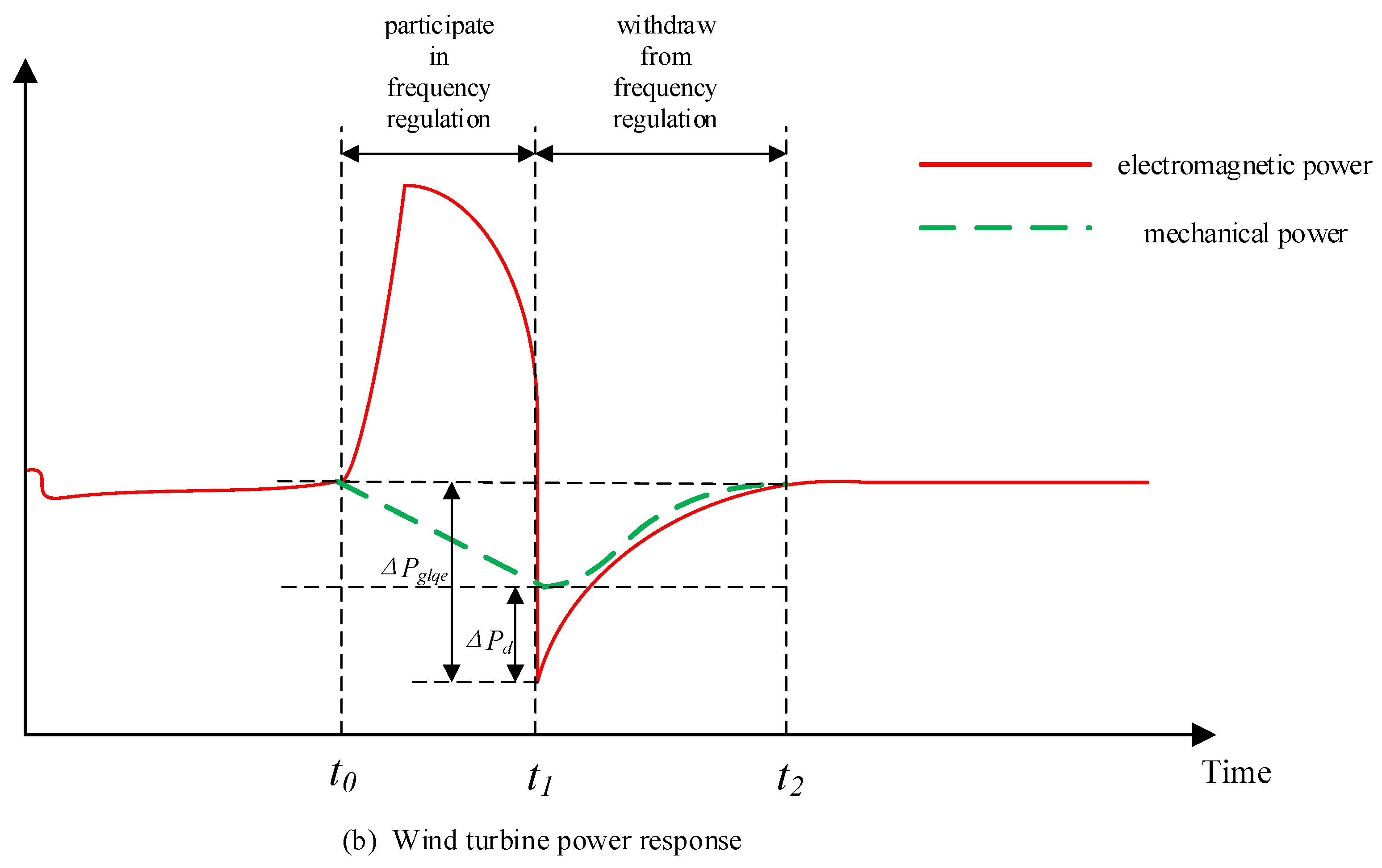
2.1. Analysis of Power Dip Phenomenon

In a doubly fed wind turbine, rotor kinetic energy can be released to temporarily boost the turbine’s electromagnetic power output and participate in power system frequency regulation. However, when the system frequency stabilizes and the frequency regulation ends, the wind turbine must quickly compensate for the rotor kinetic energy previously released during regulation. This results in the electromagnetic power output dropping sharply back to the MPPT (maximum power point tracking) curve. At this point, the mechanical power exceeds the electromagnetic power, and the difference between the mechanical and electromagnetic power, denoted as Δ P d , is used to restore the turbine’s rotor speed.
The process of wind turbine participation in primary frequency regulation and rotor speed recovery can be described as a complete cycle of 1-2-3-4-1. During the 1-2 stage, as the grid frequency drops, the wind turbine temporarily increases its electromagnetic power. In the 2-3 stage, the wind turbine releases rotor kinetic energy to participate in primary frequency regulation. During the 3-4 stage, when the grid frequency has stabilized or the rotor speed of the wind turbine becomes critically low, the turbine must replenish the rotor kinetic energy released during frequency regulation and rapidly restore its speed to avoid disconnection from the grid, which requires absorbing active power from the grid. Since wind turbines typically operate in MPPT mode, the power drops from point 3 to point 4 on the MPPT curve, resulting in a sudden decrease in the electromagnetic power output of the wind turbine, Δ P e . If N turbines shut down simultaneously, the total sudden drop in electromagnetic power would be N ×  Δ P e , which can have a significant impact on the power grid and, in severe cases, may even lead to the risk of grid collapse. Once the turbine reaches stage 4, the rotor speed begins to recover due to the difference between electromagnetic power and mechanical power. As this difference decreases, the recovery speed of the rotor gradually slows, and the turbine ultimately returns to a new stable operating point. Overall, the occurrence of the “power dip” is attributed to the lack of timely active power support for rotor speed recovery after the conclusion of system frequency regulation.

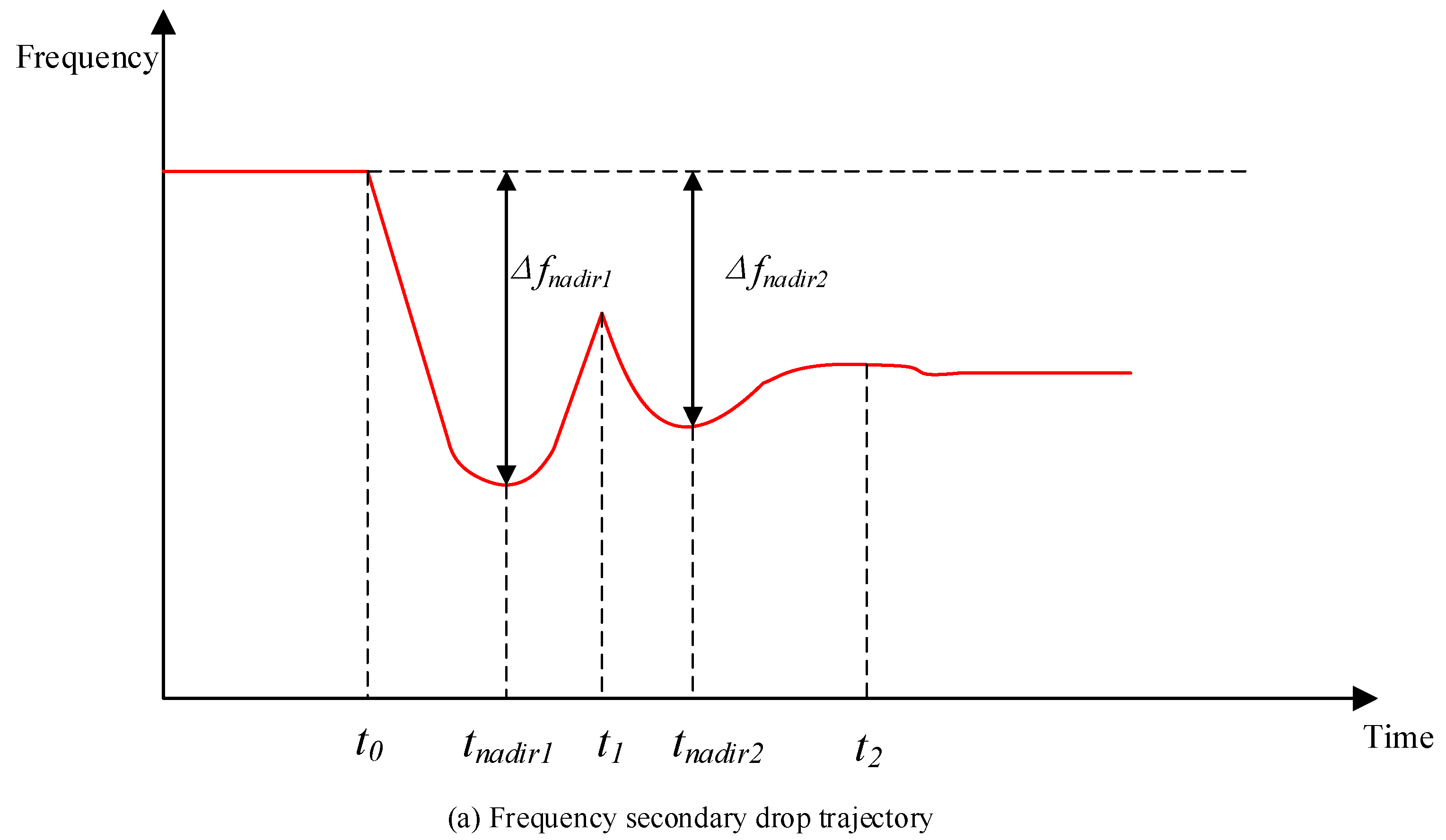
2.2. Quantification of Secondary Frequency Drop

The typical trajectory of secondary frequency drop and the corresponding power trajectory of the wind turbine are shown in Figure 1.
At time t 0 , a power disturbance P 0 occurs. t 1 marks the moment when the wind turbine exits primary frequency regulation, and t 2 is the time when the rotor speed recovery process concludes. Δ P g l q e represents the active power absorbed from the system to restore the rotor speed at the end of frequency regulation. It can also be considered the power deficit disturbance experienced by the system at that moment. As shown in the figure, following the occurrence of the power dip phenomenon, the frequency undergoes a secondary drop at time t n a d i r 2 , which further confirms the direct relationship between the secondary frequency drop and the power dip phenomenon. For the system, the power disturbance increases from P 0 to P 1 = P 0 + Δ P g l q e .
The common-mode frequency response of the power system exhibits generality, allowing a unified equivalent model to be established to represent the frequency–power relationships of various devices within the system. The expression is as follows:
G ( s ) = J u s + D u + 1 K u ( 1 + T 0 s )
In the above expression, J u , D u , and K u represent the effective inertia, effective damping coefficient, and effective static droop coefficient, respectively; T 0 denotes the droop time constant.
To quantitatively evaluate the lowest point of the secondary frequency drop, the dynamic frequency characteristic expression is provided below:
Δ f n a d i r 2 = e σ 1 ( t n a d i r 2 t 1 ) S 1 c o s h ( ω d 1 ( t n a d i r 2 t 1 ) ) +   e σ 1 ( t n a d i r 2 t 1 ) S 2 s i n h ( ω d 1 ( t n a d i r 2 t 1 ) ) P 1 D u s l + 1 K u s l
t n a d i r 2 = t 1 + 1 ω d 1 a r c t a n h S 1 σ 1 S 2 ω d 1 S 1 ω d 1 S 2 σ 1
Equations (2) and (3) represent the expressions for the maximum deviation and the specific time of the secondary frequency drop. In the equations, ω d 1 and σ d 1 are the damping oscillation coefficient and the attenuation coefficient during the secondary frequency drop process of the system, respectively, and their expressions are as follows:
ω d 1 = ( D u s 1 T 0 J u s 1 ) 2 4 J u s 1 T 0 K u s 1 2 J u s 1 T 0 σ 1 = J u s 1 + D u s 1 T 0 2 J u s 1 T 0
Here, J u s 1 , D u s 1 , and K u s 1 are the unified structural parameters during the secondary frequency drop. Parameters S 1 and S 2 are related to J u s 1 , D u s 1 , K u s 1 , and t 1 , with their expressions being as follows:
S 1 = Δ f t 1 + P 1 D u s l + 1 / K u s l S 2 = J u s l D u s l T 0 Δ f t 1 2 J u s l T 0 ω d 1 + P 1 J u s l 2 D u s l T 0 2 T 0 / K u s l D u s l + 1 / K u s l ω d 1 J u s l T 0
The calculation process can be summarized in the following steps:
  • Step 1: Obtain the unified structural parameters of the system.
  • Step 2: Determine key settings such as the wind power disconnection time and the magnitude of the power deficiency disturbance.
  • Step 3: Substitute these values into Equations (4) and (5) to calculate the intermediate parameters: S 1 , S 2 , ω d 1 , σ 1 .
  • Step 4: Insert the obtained parameters into Equations (2) and (3) to derive the time of the secondary frequency dip and the corresponding frequency nadir.

3. Two-Stage Scheduling Model

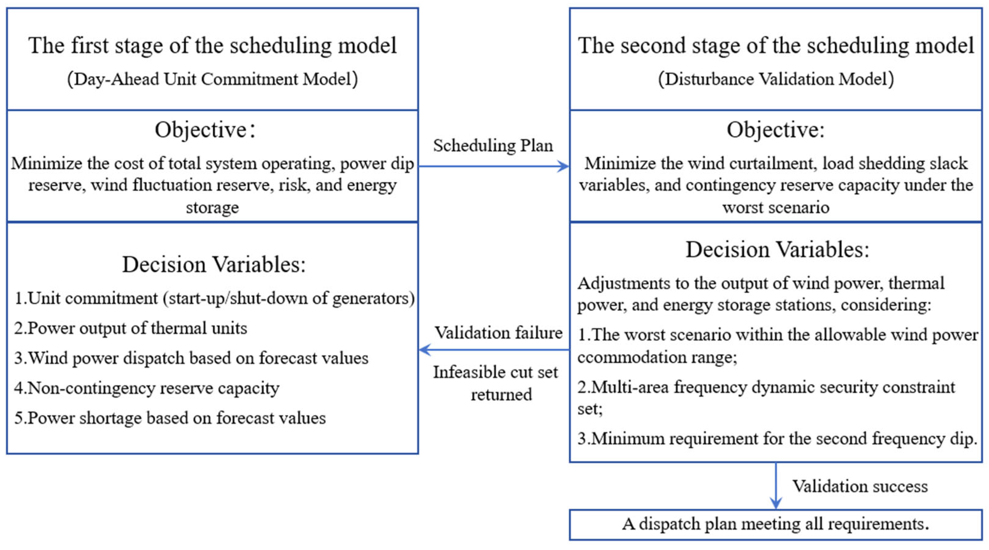
3.1. Overall Framework of the Scheduling Model

To enhance the comprehensiveness and coherence of the scheduling model, it is divided into two stages to address the unit output scheduling problem and frequency security verification under the worst-case scenario. The framework of the scheduling model is shown in Figure 2.
The first stage of the scheduling model is risk-based scheduling based on wind power forecasts. Given the load and wind power values, network topology, and power disturbances, the model fully considers the safety and economic aspects of the scheduling process to derive the optimal scheduling scheme through iterative optimization.
The second stage focuses on predictive disturbance detection for multi-area frequency security. The scheduling results from the first stage, such as unit start-up and shutdown status, allowable wind power absorption range, and reserve capacity, are used as inputs for large power disturbance frequency security detection in the second stage. If the detection is successful, the current scheduling scheme is output as the optimal solution. If the detection fails, an infeasible cut set is returned for further iterative optimization. The model can also be simplified into a two-layer optimization framework consisting of pre-scheduling and re-scheduling.
In the optimization of unit reserve capacity, the model decouples reserve capacity into power dip reserve and wind fluctuation reserve. The former addresses power deficits arising during the transition of wind turbines from primary frequency regulation to normal operation, while the latter compensates for fluctuations in wind power output. In the first stage, the model determines the power dip reserve and wind fluctuation reserve, while the second stage involves verification and validation of the reserve capacity.

3.2. First-Stage Scheduling

3.2.1. Objective Function for the First-Stage Scheduling

The objective function of the pre-scheduling stage consists of four components: the total operating cost of the system, the cost of wind fluctuation reserve, the cost of power dip reserve, and operational risk.
min t T k K ( C k , t P + C k , t U + c k R + R k , t + + c k R R k , t + c k R + R g l k , t + ) + ε R I S K
In the above expression, C k , t P represents the operating cost of thermal power units, which is modeled using a piecewise linearization approach [13], while C k , t U denotes the startup cost of the units, with the shutdown cost considered negligible. c k R + and c k R correspond to the unit costs for upward and downward reserve capacity of thermal power units, respectively. R k , t + , R k , t , and R g l k , t + represent the positive wind fluctuation reserve capacity, negative wind fluctuation reserve capacity, and power dip reserve capacity, respectively. ε is the risk cost coefficient, and R I S K represents the system’s operational risk cost, which accounts for potential risks of wind curtailment or load shedding caused by the uncertainty of wind power output. Assuming a given unit cost for wind curtailment and load shedding, and that wind power output at each time step follows a normal distribution with the current forecasted value as its mean, the conditional value-at-risk (CVaR) theory is applied. When wind power output exceeds its upper limit, there is a risk of wind curtailment, leading to wind curtailment risk costs. Conversely, when wind power output falls below its lower limit, there is a risk of load shedding, resulting in load shedding risk costs. The expression for the system’s operational risk cost is presented in Equation (7).
R I S K = t T w W ( c w c u r C V a R w , t + + c w l o s s C V a R w , t )
In the equation, c w c u r and c w l o s s denote the unit risk cost of wind power curtailment and the unit risk cost of load loss, respectively, while C V a R w + and C V a R w denote the wind power curtailment risk and the load loss risk, respectively.

3.2.2. First-Stage Scheduling Constraints

(1)
Generation capacity limits of thermal power units
P k , t 0 = u k , t P _ k , t + l = 1 L P k , t , l 0 P k , t , l u k , t P ¯ k , l P ¯ k , l = ( P ¯ k P _ k ) / L
In the above equation, L denotes the number of piecewise linear segments for the thermal power unit; P k , t , l represents the output value of each segment; u k , t is the binary start-up/shutdown decision variable of unit k at time t; P k , t 0 denotes the output of thermal unit k during the pre-dispatch stage; P k ¯ and P _ k represent the lower and upper generation limits of the thermal unit, respectively. The superscript 0 indicates variables corresponding to the pre-dispatch stage.
(2)
Ramping constraints for thermal power units
D R k Δ t P k , t 0 P k , t 1 0 U R k Δ t
In the above equation, D R k and U R k represent the ramp-down rate and ramp-up rate, respectively, while Δ t denotes the dispatch time interval.
(3)
Wind power fluctuation reserve and power dip reserve constraints
u k , t P _ k P k , t 0 + R k , t + + R g l k , t + u k , t P ¯ k u k , t P _ k P k , t 0 R k , t u k , t P ¯ k R k , t + , R k , t , R g l k , t + 0 R g l k , t + P g l q e , t P k , t 0 + R k , t + + R g l k , t + ( P k , t + 1 0 R k , t + 1 ) u k , t + 1 D R k Δ t + ( 1 u k , t + 1 ) P ¯ k P k , t + 1 0 + R k , t + 1 + + R g l k , t + 1 + ( P k , t 0 R k , t ) u k , t U R k Δ t + ( 1 u k , t ) P ¯
Among these equations, the first four constrain the reserve capacity, while the last two impose ramp rate constraints on the generating units. In the equations, R g l k , t + represents the power dip reserve provided by the unit, and P g l q e , t denotes the power deficit at each time period that leads to the power dip phenomenon in the system.
(4)
Constraints on wind power generation output
0 P w , t 0 P w , t p r e 0 P w , t p r e P w , t P w , t 0 P w , t p r e + P w , t + P ¯ w
In the above equation, P w , t 0 denotes the wind power output in the pre-dispatch stage; P w , t p r e is the forecasted wind power output; P w , t + and P w , t represent the lower and upper fluctuation bounds of wind power output, respectively; and P ¯ w denotes the maximum wind power output.
(5)
Active power balance constraint
k = 1 K s e P k , t 0 + w = 1 W s e P w , t 0 c = 1 C P c , t 0 = d = 1 D s e P d , t
k = 1 K r e P k , t 0 + w = 1 W r e P w , t 0 + c = 1 C P c , t 0 = d = 1 D r e P d , t
Equations (12) and (13) represent the active power balance constraints for the sending-end and receiving-end systems, respectively. In these equations, the superscript se denotes variables associated with the sending-end system, while re indicates those related to the receiving-end system. K, W, D, and C represent the sets of thermal units, wind farms, load nodes, and tie-lines, respectively. P d , t denotes the load demand.
(6)
DC power flow constraints for the sending-end and receiving-end grids
F ¯ k K K se Υ k P k , t 0 + w W W se Υ w P w , t 0 c C Υ c P c , t 0 d D D s Υ d P d , t F ¯
F ¯ k K K re Υ k P k , t 0 + w W W re Υ w P w , t 0 + c C Υ c P c , t 0 d D D re Υ d P d , t F ¯
In the above equation, Υ k , Υ w , Υ c , and Υ d are the power transfer distribution factors (PTDFs) for thermal power units, wind power units, tie-lines, and load nodes, respectively; F ¯ denotes the transmission capacity limit of the branch.
(7)
Tie-line transmission power constraint
0 R c , t + , R c , t R ¯ c . t P c , t 0 + R c , t + P ¯ c P c . t 0 R c . t 0 P c , t 0 + R c , t + ( P c . t + 1 0 R c , t + 1 ) ξ + P c , t + 1 0 + R c , t + 1 + ( P c . t 0 R c . t ) ξ
The first three equations constrain the magnitude of the tie-line transmission power, while the last two impose constraints on the ramping rate of tie-line power adjustments. In the equations, R c , t + and R c , t denote the upward and downward regulation margins of tie-line transmission power; P ¯ c represents the maximum transmission capacity of the tie-line; and ξ + and ξ indicate the limits of upward and downward power adjustments per unit time.

3.3. Second-Stage Scheduling

3.3.1. Objective Function for the Second-Stage Scheduling

The re-dispatch stage is essentially a robust optimization-based validation process under anticipated disturbances. Slack variables representing wind power curtailment and load shedding are introduced, and the objective function is formulated to minimize the sum of these slack variables under the worst-case wind power scenario. During the iterative solution process, if the sum of the slack variables is zero, it indicates that the dispatch plan obtained from the pre-dispatch stage satisfies the frequency security constraints under the worst-case scenario, with no risk of wind curtailment or load shedding.
Since the re-dispatch stage constitutes a bi-level max–min problem, it must be transformed into a single-level maximization problem using strong duality theory in order to be solvable by commercial optimization solvers. The objective function of the re-dispatch stage is formulated as follows:
max P w min t T [ w ( W se W re ) Δ P w , t u + d ( D se D re ) Δ P d , t u ]
In the equation, Δ P w , t u and Δ P d , t u are slack variables representing wind power curtailment and load shedding, respectively.

3.3.2. Second-Stage Scheduling Constraints

(1)
Power balance constraint
k = 1 K s e P k , t u + w = 1 W s e ( P w , t p r e , u Δ P w , t u ) c = 1 C P c , t u = d = 1 D s e ( P d , t Δ P d , t u )
k = 1 K r e P k , t u + w = 1 W r e ( P w , t p r e , u Δ P w , t u ) + c = 1 C P c , t u = d = 1 D r e ( P d , t Δ P d , t u )
In the equation, the superscript u denotes variables associated with the re-dispatch stage.
(2)
DC power flow constraints
F ¯ k K K s e Υ k P k , t u + w W W s e Υ w ( P w , t p r e , u Δ P w , t u ) c C Υ c P c , t u d D D s e Υ d ( P d , t Δ P d , t u ) F ¯
F ¯ k K K r e Υ k P k , t u + w W W r e Υ w ( P w , t p r e , u Δ P w , t u ) + c C Υ c P c , t u d D D r e Υ d ( P d , t Δ P d , t u ) F ¯
(3)
Thermal unit output adjustment constraints
P k , t 0 R k , t P k , t u P k , t 0 + R k , t + + R g l k , t +
(4)
Tie-line power transfer adjustment constraints
P c , t 0 R c , t P c , t u P c , t 0 + R c , t +
(5)
Slack variable constraints for wind curtailment and load shedding
0 Δ P w , t u P w , t p r e , u 0 Δ P d , t u P d , t
(6)
Uncertainty set of wind power output
In robust optimization, the uncertainty set is used to characterize all possible realizations of uncertain parameters. In this study, a polyhedral uncertainty set is constructed for the dynamic optimization of wind power accommodation intervals, considering both temporal and zonal dimensions, as follows:
P W u = { P w , t u | P w , t u = P w , t 0 + z w , t u , + Δ P w , t + z w , t u , Δ P w , t w = 1 W ( z w , t u , + + z w , t u , ) Γ S , t = 1 T ( z w , t u , + + z w , t u , ) Γ T z w , t u , + + z w , t u , 1 , w , t , z w , t u , + , z w , t u , { 0 , 1 } }
In the equation, z w , t u , + and z w , t u , are binary variables indicating upward and downward wind power adjustments, respectively, with, at most, one of them being equal to 1 at any given time. Γ S and Γ T represent the spatial and temporal uncertainty budgets, respectively, whose calculation is provided in Equation (26). Δ P w , t + and Δ P w , t denote the upward and downward adjustment amounts of wind power output, respectively, with their expressions defined in Equation (27).
Γ S = Φ 1 ( 1 α ) W Γ T = Φ 1 ( 1 α ) T
In the equation, Φ denotes the cumulative distribution function (CDF) of the normal distribution; α is the predefined significance level; W represents the number of wind farms; and T is the number of dispatch time intervals.
Δ P w , t + = P w , t p r e + P w , t + P w , t 0 Δ P w , t = P w , t 0 P w , t p r e + P w , t
(7)
Secondary frequency dip security constraint
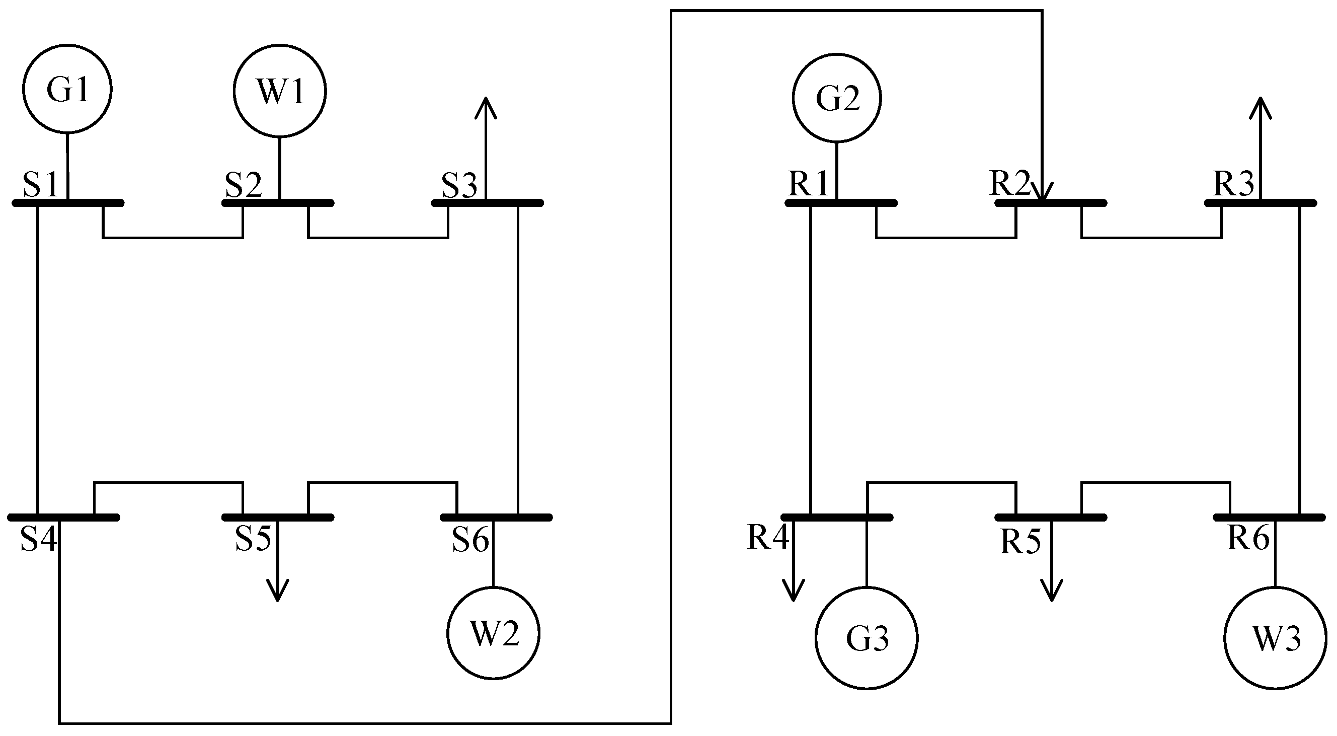
In the anticipated disturbance verification of the secondary frequency dip security constraint in the second-stage dispatch, it is assumed that the frequency disturbance at each time interval corresponds to 10% of the total load in the region. Based on the unit commitment and generation output obtained from the first-stage dispatch, the minimum value of the secondary frequency dip is evaluated to determine whether it meets the specified security requirements.
f n a d i r 2 f n a d i r 2 min
t n a d i r 2 t n a d i r 2 min
Equations (2), (3), (28), and (29) jointly constitute the secondary frequency dip security constraint.

4. Case Study

To verify the feasibility of the proposed model, a two-area 12-bus system, as illustrated in Figure 3, is used as a case study. The 12-bus system simulates the actual spatial distribution of wind farms. The left side represents the sending-end system, while the right side represents the receiving-end system, interconnected through a tie-line. The maximum transmission capacity of the tie-line is set to 200 MW, and the power ramping rate is limited to 15% of this maximum capacity. A power deficit disturbance is applied in the receiving-end system, with the disturbance magnitude set to 10% of the total load in that area at each time interval. The RoCoF (Rate of Change of Frequency) limit at the initial moment is set to 1 Hz/s, the minimum frequency threshold is set to 49.2 Hz, and the quasi-steady-state frequency is set to 49.5 Hz. The power deficit caused by the withdrawal of wind turbines from frequency regulation is assumed to be 7% of the total predicted wind power output at the given time, with a ±5% fluctuation range allowed. The sending-end system consists of one thermal unit (G1) with a rated capacity of 200 MVA and two wind farms (WT1 and WT2), each rated at 100 MVA. The receiving-end system comprises a 200 MVA thermal plant (G2), a 300 MVA thermal plant (G3), and a 100 MVA wind farm (WT3). The unit wind curtailment cost is set at USD 50/(MW·h), and the load shedding penalty is also USD 50/(MW·h). The risk cost coefficient ε is set to 1. The structural parameters of all devices used in this case are listed in Table 1.

4.1. Economic Impact of Scheduling in Multi-Area Systems

To analyze the impact of scheduling strategies on the economic performance of multi-area power systems, the following two scheduling modes are defined:
Mode 1: In the multi-area scheduling system, the power dip phenomenon is not optimized, and no power dip reserve is allocated.
Mode 2: In the multi-area scheduling system, the power dip phenomenon is explicitly optimized, and a dedicated power dip reserve is allocated.
Table 2 presents the economic cost results of system operation under different scheduling modes. In terms of total cost, Mode 1 exhibits a lower overall cost compared to Mode 2. The primary difference arises from the inclusion of power dip reserve in Mode 2, which increases its economic cost. In Mode 2, the thermal power reserve capacity is reallocated, and a dedicated power dip reserve is established independently. As a result, the reserve capacity available to respond to wind power fluctuations is reduced, leading to slightly higher wind curtailment and load shedding risk costs in Mode 2 compared to Mode 1.
The detailed economic costs for each region under different dispatching modes are presented in Table 3. It can be observed that the operating costs of thermal power units in both the sending and receiving regions are relatively similar between Mode 1 and Mode 2. However, the reserve cost in the sending region under Mode 2 is higher than that under Mode 1. This is primarily because Mode 2 accounts for power dip reserves, and the sending region has a higher proportion of wind power. Consequently, a larger amount of reserve capacity is required in this region, leading to higher reserve costs in Mode 2 compared to Mode 1.

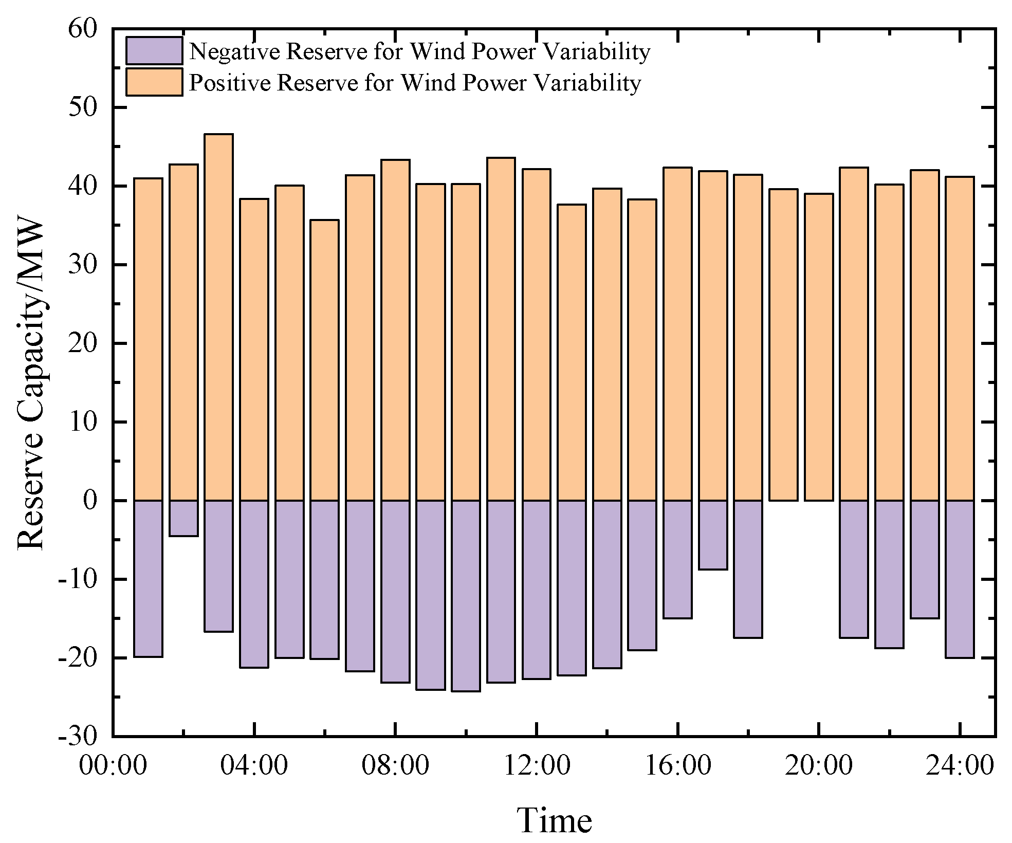
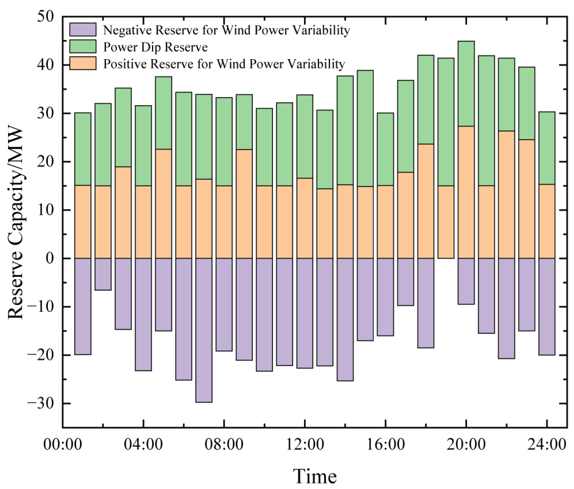
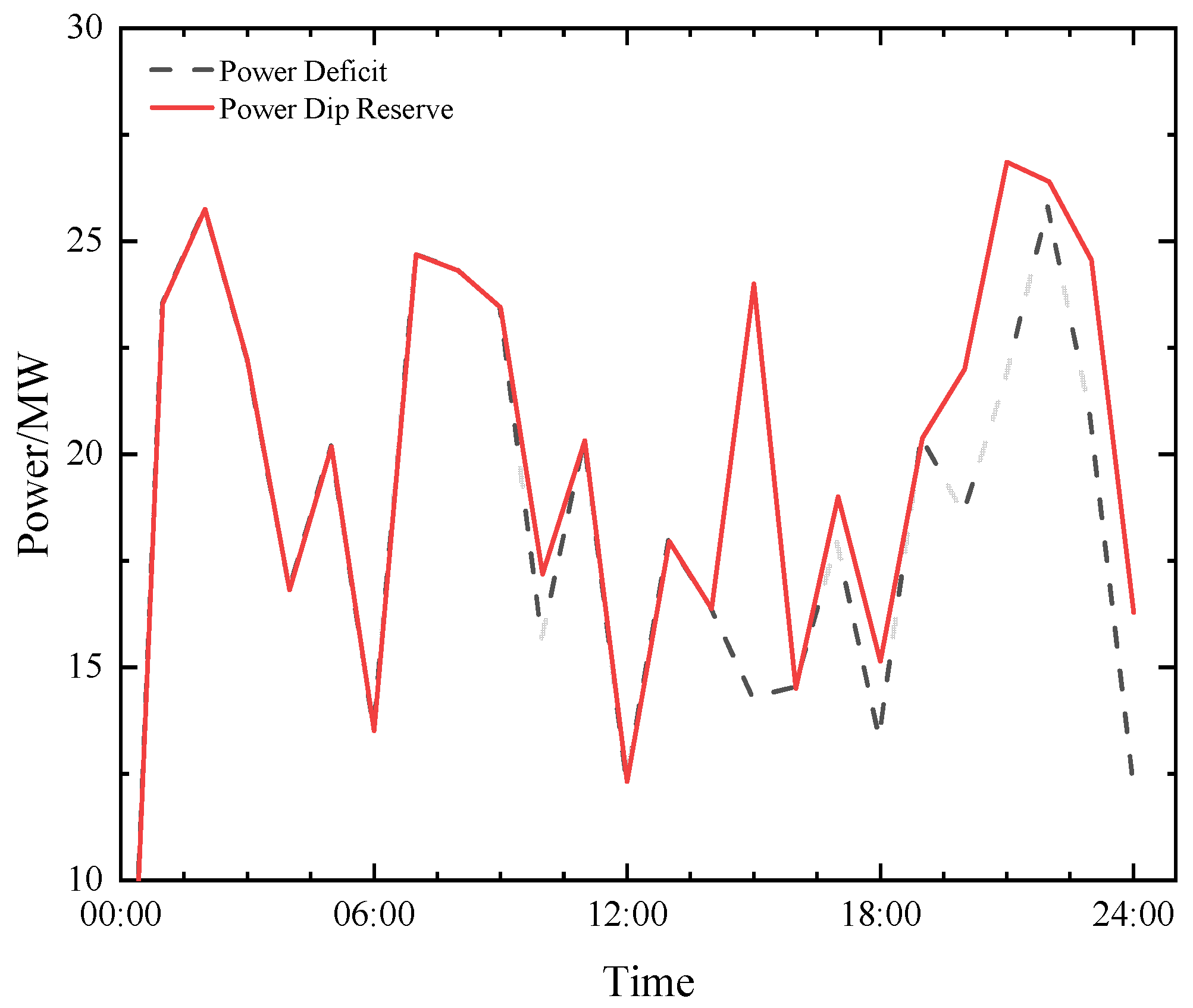
4.2. Impact of Scheduling Strategies on Reserve Capacity Allocation

Different scheduling strategies have a significant impact on the allocation of various types of reserve capacity in the system. Figure 4 and Figure 5 represent the reserve capacity distributions under Scheduling Mode 1 and Mode 2, respectively. In the figure, green indicates the power dip reserve, purple denotes the downward reserve for wind power fluctuation, and yellow represents the upward reserve for wind power fluctuation. It can be observed that, in response to the varying levels of anticipated power disturbances, Mode 2 allocates power dip reserves to address potential frequency security issues. Additionally, it is evident that the total amount of upward reserve obtained through optimization in Modes 1 and 2 is relatively similar. However, due to the explicit consideration of power dip reserves in Mode 2, there is a significant difference in the specific allocation of upward reserve capacity between the two modes.

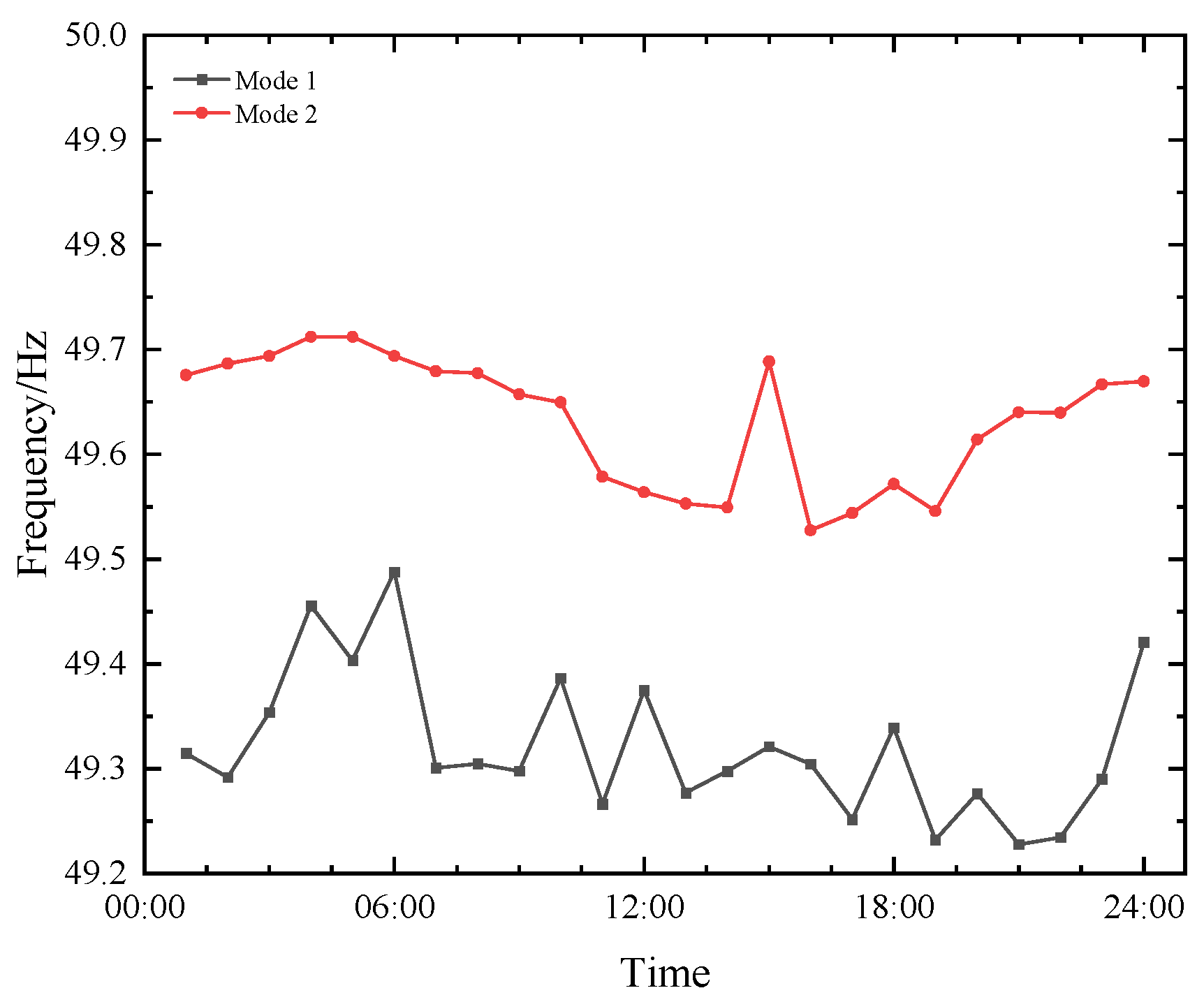
4.3. Impact of Scheduling Strategies on the Nadir of Secondary Frequency Drop

To verify whether the scheduled power dip reserve is sufficient to fully compensate for the power deficit caused by large-scale withdrawal of wind turbines from frequency regulation, the relationship between the power deficit and the power dip reserve determined by the scheduling model is calculated. The results are shown in Figure 6.
The red solid line represents the power dip reserve scheduled by the model, while the black dashed line denotes the actual power deficit in the system. Although the power deficit is allowed to fluctuate randomly within a certain range, the power dip reserve curve remains highly synchronized with the power deficit curve—it either overlaps with or slightly exceeds it at all times. This indicates that the power dip reserve provided by the scheduling model can reliably track the power deficit and reasonably compensate for it.
To evaluate the effectiveness of scheduling strategies in mitigating the severity of secondary frequency dips, Figure 7 illustrates the nadir of the secondary frequency drop at each time interval under different scheduling modes (Modes 1 and 2). It can be observed that, under the same power disturbance, the nadir frequencies in Mode 1 are generally lower. Specifically, during the dispatch period from 19:00 to 23:00, the minimum frequency approaches 49.2 Hz—the predefined lower frequency threshold—posing a high risk of triggering under-frequency load shedding. This is primarily because Mode 1 does not allocate power dip reserves independently, and therefore, it fails to promptly deploy sufficient reserves to maintain power balance when wind units withdraw from frequency regulation. In contrast, Mode 2 shows a significant improvement in maintaining higher frequency nadirs, generally above 49.5 Hz. This indicates a reduced risk of UFLS and demonstrates that Mode 2 more effectively optimizes the system’s response to secondary frequency dips, thereby enhancing frequency security.
As shown in Table 4, the nadir frequency in Mode 2 is significantly higher than that in Mode 1, and the arrival time of the secondary frequency dip is notably delayed, indicating that the proposed method of decoupling thermal unit reserves to mitigate the power dip phenomenon is effective.

5. Conclusions

This study constructs a multi-area optimal scheduling model considering secondary frequency dips, integrating multi-area frequency security constraints and the primary frequency regulation characteristics of DFIGs. A two-area, 12-bus case study validates the effectiveness of the model. The following key conclusions are drawn:
(1) By quantifying the balance between scheduling conservatism and risk sensitivity through a risk cost coefficient, the model determines an optimal trade-off point between unit commitment costs and conditional value-at-risk (CVaR)-based risk loss costs. This mechanism enables the derivation of economically viable and risk-constrained scheduling schemes for renewable energy units, ensuring operational robustness under uncertain wind power outputs.
(2) The proposed model innovatively decouples system reserve capacity into scenario-specific components based on disturbance characteristics. As frequency security requirements intensify, the model dynamically optimizes inter-area reserve distribution, which increases scheduling costs, but it achieves a systematic balance between reserve efficiency and frequency stability. This adaptive allocation strategy outperforms traditional uniform reserve planning by aligning resources with dynamic operational demands.
(3) The introduced power dip reserve effectively compensates for the power deficit caused by DFIGs reverting from primary frequency regulation to normal operation. By addressing the power dip phenomenon, the model elevates the minimum point of secondary frequency dips and reduces their severity, providing a practical scheduling-level solution to enhance transient frequency security in high-penetration wind power systems.
Although this study achieves promising results in enhancing system frequency security, several limitations remain. The model does not yet incorporate energy storage systems, thus overlooking their fast response capability. It also treats multi-area systems as frequency-coherent, without capturing possible inter-regional frequency dynamics. Furthermore, the spatial and temporal characteristics of load behavior are not considered in the modeling of load-side regulation. These aspects will be explored in future work to improve the model’s adaptability and practical applicability.

Author Contributions

Conceptualization, X.Y. and T.W.; formal analysis, L.C.; methodology, X.Y. and X.H.; software, L.C.; supervision, T.W.; validation, Y.S.; writing—original draft, X.H.; writing—review and editing, T.W. and Y.S. All authors have read and agreed to the published version of the manuscript.

Funding

This project is supported by the State Grid Hebei Electric Power Co., Ltd. Technology Project (grant No. kj2024-001).

Data Availability Statement

The data presented in this study are available on request from the corresponding author.

Conflicts of Interest

Authors Xiaodong Yang, Lun Cheng and Yujing Su are employed by State Grid Hebei Electric Co. Ltd. The remaining authors declare that the research was conducted in the absence of any commercial or financial relationships that could be construed as a potential conflict of interest.

References

  1. Kang, C.; Yao, L. Key Scientific Issues and Theoretical Research Framework for Power Systems with High Proportion of Renewable Energy. Autom. Electr. Power Syst. 2017, 41, 2–11. [Google Scholar]
  2. Zheng, Y.; Li, Z.; Chai, J. Progress and prospects of international carbon peaking and carbon neutral research—Based on bibliometric analysis (1991–2022). Front. Energy Res. 2023, 11, 1121639. [Google Scholar] [CrossRef]
  3. Ma, R.; Zhan, M.; Jiang, K.; Liu, D.; Hu, P.; Cheng, S. Transient Stability Assessment of Renewable Dominated Power Systems by the Method of Hyperplanes. IEEE Trans. Power Deliv. 2023, 38, 3455–3468. [Google Scholar] [CrossRef]
  4. Janusz, B. What does the GB power outage on 9 August 2019 tell us about the current state of decarbonised power systems? Energy Policy 2020, 146, 111821. [Google Scholar] [CrossRef]
  5. Yan, R.; Al Masood, N.; Kumar Saha, T.; Bai, F.; Gu, H. The Anatomy of the 2016 South Australia Blackout: A Catastrophic Event in a High Renewable Network. IEEE Trans. Power Syst. 2018, 33, 5374–5388. [Google Scholar] [CrossRef]
  6. Zhou, D.; Zou, Z.; Dan, Y.; Wang, C.; Teng, C.; Zhu, Y. An Integrated Strategy for Hybrid Energy Storage Systems to Stabilize the Frequency of the Power Grid Through Primary Frequency Regulation. Energies 2025, 18, 246. [Google Scholar] [CrossRef]
  7. Ratnam, K.S.; Palanisamy, K.; Yang, G. Future low-inertia power systems: Requirements, issues, and solutions—A review. Renew. Sustain. Energy Rev. 2020, 124, 109773. [Google Scholar] [CrossRef]
  8. Zou, S.; Zong, X.; Chen, Q.; Zhang, W.; Zhou, H. Optimization Scheduling of Integrated Energy Systems Considering Power Flow Constraints. Energies 2025, 18, 2442. [Google Scholar] [CrossRef]
  9. Chen, Y.; Zhao, Y.; Zhang, X.; Wang, Y.; Mi, R.; Song, J.; Hao, Z.; Xu, C. A Two-Stage Robust Optimization Strategy for Long-Term Energy Storage and Cascaded Utilization of Cold and Heat Energy in Peer-to-Peer Electricity Energy Trading. Energies 2025, 18, 323. [Google Scholar] [CrossRef]
  10. Jin, W.; Wang, P.; Yuan, J. Key Role and Optimization Dispatch Research of Technical Virtual Power Plants in the New Energy Era. Energies 2024, 17, 5796. [Google Scholar] [CrossRef]
  11. Zeng, B.; Zhao, L. Solving two-stage robust optimization problems using a column-and-constraint generation method. Oper. Res. Lett. 2013, 41, 457–461. [Google Scholar] [CrossRef]
  12. Tsang, M.Y.; Shehadeh, K.S.; Curtis, F.E. An inexact column-and-constraint generation method to solve two-stage robust optimization problems. Oper. Res. Lett. 2023, 51, 92–98. [Google Scholar] [CrossRef]
  13. Roald, L.A.; Pozo, D.; Papavasiliou, A.; Molzahn, D.K.; Kazempour, J.; Conejo, A. Power systems optimization under uncertainty: A review of methods and applications. Electr. Power Syst. Res. 2023, 214, 108725. [Google Scholar] [CrossRef]
  14. Guan, Y.; Wang, J. Uncertainty sets for robust unit commitment. IEEE Trans. Power Syst. 2014, 29, 1439–1440. [Google Scholar] [CrossRef]
  15. Wu, W.; Wang, K.; Li, G.; Ge, Y. Modeling ellipsoidal uncertainty set considering conditional correlation of wind power generation. Proc. CSEE 2017, 37, 2500–2507. [Google Scholar]
  16. Wu, Z.; Chen, C.; Xu, D.; Guan, L. Frequency-Constrained Economic Dispatch of Microgrids Considering Frequency Response Performance. Energies 2025, 18, 2014. [Google Scholar] [CrossRef]
  17. Teng, F.; Trovato, V.; Strbac, G. Stochastic scheduling with inertia-dependent fast frequency response requirements. IEEE Trans. Power Syst. 2016, 31, 1557–1566. [Google Scholar] [CrossRef]
  18. Zhou, Z.; Wang, Z.; Zhang, Y.; Wang, X. Nash Bargaining-Based Coordinated Frequency-Constrained Dispatch for Distribution Networks and Microgrids. Energies 2024, 17, 5661. [Google Scholar] [CrossRef]
  19. Badesa, L.; Teng, F.; Strbac, G. Simultaneous scheduling of multiple frequency services in stochastic unit commitment. IEEE Trans. Power Syst. 2019, 34, 3858–3868. [Google Scholar] [CrossRef]
  20. Badesa, L.; Teng, F.; Strbac, G. Conditions for Regional Frequency Stability in Power System Scheduling—Part I: Theory. IEEE Trans. Power Syst. 2021, 36, 5558–5566. [Google Scholar] [CrossRef]
  21. Badesa, L.; Teng, F.; Strbac, G. Conditions for Regional Frequency Stability in Power System Scheduling—Part II: Application to Unit Commitment. IEEE Trans. Power Syst. 2021, 36, 5567–5577. [Google Scholar] [CrossRef]
  22. Qian, M.; Wang, J.; Yang, D.; Yin, H.; Zhang, J. An Optimization Strategy for Unit Commitment in High Wind Power Penetration Power Systems Considering Demand Response and Frequency Stability Constraints. Energies 2024, 17, 5725. [Google Scholar] [CrossRef]
  23. Zhang, G.; Ela, E.; Wang, Q. Market Scheduling and Pricing for Primary and Secondary Frequency Reserve. IEEE Trans. Power Syst. 2019, 34, 2914–2924. [Google Scholar] [CrossRef]
  24. Xin, X.; Wang, T.; Gu, X.; Bai, Y.; Fan, H. Unit Commitment and Risk Dispatch Considering Multi-Regional Frequency Dynamic Security Under Large-Scale Wind Power Access. Proc. CSEE 2023, 43, 5824–5839. [Google Scholar]
  25. Wu, S.; Mu, R.; Zhang, Y.; Song, H.; Zhao, W.; Huang, K.; Zhu, B. Study of Power Pit in System Frequency Modulation of Doubly-Fed Induction Generator. Electr. Power Sci. Eng. 2021, 37, 1–11. [Google Scholar]
  26. Zhang, W.; Wu, C.; Huang, W.; Gao, H.; Cheng, M.; Xin, H. Evaluation of System Frequency Characteristic and Parameter Setting of Frequency Regulation for Wind Power Considering Secondary Frequency Drop. Autom. Electr. Power Syst. 2022, 46, 11–19. [Google Scholar]
  27. Liu, K.; Qu, Y.; Kim, H.-M.; Song, H. Avoiding Frequency Second Dip in Power Unreserved Control During Wind Power Rotational Speed Recovery. IEEE Trans. Power Syst. 2018, 33, 3097–3106. [Google Scholar] [CrossRef]
  28. Li, D.; Wan, R.; Xu, B.; Yao, Y.; Dong, N.; Zhang, X. Optimal Capacity Configuration of the Wind-Storage Combined Frequency Regulation System Considering Secondary Frequency Drop. Front. Energy Res. 2023, 11, 1037587. [Google Scholar] [CrossRef]
  29. Cheng, Y.; Sun, H.; Zhang, Y.; Xu, S.; Zhao, B.; Vorobev, P.; Terzija, V. A consecutive power dispatch in wind farms to mitigate secondary frequency dips. Int. J. Electr. Power Energy Syst. 2024, 158, 109939. [Google Scholar] [CrossRef]
Figure 1. Simulation curve of wind turbine speed recovery process. (a) Frequency secondary drop trajectory; (b) wind turbine power response.
Energies 18 03926 g001aEnergies 18 03926 g001b
Figure 2. Schematic diagram of a two-stage scheduling model.
Energies 18 03926 g002
Figure 3. Two-region 12-node system.
Energies 18 03926 g003
Figure 4. Primary reserve capacity in Mode 1.
Energies 18 03926 g004
Figure 5. Primary reserve capacity in Mode 2.
Energies 18 03926 g005
Figure 6. Plot of power deficit versus power dip reserve size.
Energies 18 03926 g006
Figure 7. The lowest point of the second decrease in the system frequency in different scheduling modes.
Energies 18 03926 g007
Table 1. Equivalent parameters of the same structure.
ParametersG1G2G3WT1WT2WT3
Jul13.9413.9419.9112.612.612.6
Dul11.4611.4617.1917.9317.9317.93
1/Kul12.3612.3618.54−3.1−3.1−3.1
T0555555
Table 2. Comparison of economic costs of different dispatch models.
ModeOperating Cost/USDCost of Reserves for Wind Power Variability/USDPower Dip Reserve Cost/USDWind Curtailment and Load Shedding Risk/USDTotal Cost/USD
1104,620984901354115,823
2105,817642340581862118,160
Table 3. Comparison of economic performance across different regions.
ModeOperating Cost in Sending Region/USDOperating Cost in Receiving Region/USDTotal Reserve Cost in the Sending Region/USDTotal Reserve Cost in the Receiving Region/USD
149,21755,40365753274
248,99756,82083392142
Table 4. Comparison of frequency secondary drop characteristics under different scheduling modes.
ModeTotal Cost/USDThe Lowest Value of Frequency Secondary Drop/HzFrequency Secondary Drop Time/s
1115,82349.237.52
2118,16049.577.80
Disclaimer/Publisher’s Note: The statements, opinions and data contained in all publications are solely those of the individual author(s) and contributor(s) and not of MDPI and/or the editor(s). MDPI and/or the editor(s) disclaim responsibility for any injury to people or property resulting from any ideas, methods, instructions or products referred to in the content.

