Coordination of Hydropower Generation and Export Considering River Flow Evolution Process of Cascade Hydropower Systems

Abstract

Focusing the over simplification of existing models in simulating river flow evolution process and lack of coordination of hydropower generation and export, this paper proposes a hydropower generation and export coordinated optimal operation model that, at the same time, incorporates dynamic water flow delay by finely modeling the water flow evolution process among cascade hydropower stations within a river basin. Specifically, firstly, a dynamic water flow evolution model is built based on the segmented Muskingum method. By dividing the river into sub-segments and establishing flow evolution equation for individual sub-segments, the model accurately captures the dynamic time delay of water flow. On this basis, integrating cascade hydropower systems and the transmission system, a hydropower generation and export coordinated optimal operation model is proposed. By flexibly adjusting the power export, the model balances local consumption and external transmission of hydropower, enhancing the utilization efficiency of hydropower resources and achieving high economic performance. A case study verified the accuracy of the dynamic water flow evolution model and the effectiveness of the proposed hydropower generation and export coordinated optimal operation model.

1. Introduction

With the rapid development of renewable energy, the optimal scheduling of cascade hydropower systems in river basins, which is a mainstay of renewable energy, has become an important focus of research in the hydropower field. As a crucial component of renewable energy, the efficient and stable operation of cascade hydropower stations is of great significance for improving energy utilization and ensuring the stability of the entire power system [1,2,3,4,5]. In cascade hydropower systems, hydraulic and electrical interactions exist across different stations [6]. The available water of downstream hydropower stations for power generation is influenced by both the water discharge from the upstream stations and the natural inflow from regional rivers. Moreover, the water flow from the upstream undergoes a dynamic evolution process, and accurately capturing the evolution process, particularly the accompanied time-delay effect, is crucial for avoiding inaccurate and even infeasible scheduling outcomes [7]. In fact, taking into account the time-delay effect associated with the dynamic evolution process of water flow has become necessary [8,9,10].

Reference [11] proposed an optimization model for the long-term scheduling of a hydropower cascade system located in Switzerland, focusing on addressing the issue of water flow delay. The model divides the reservoir-based hydropower stations into several hydraulically independent subsystems and introduces time-delay parameters to simulate the delay in upstream water flow reaching downstream hydropower stations, thereby improving the modeling accuracy of water balance evolution. Reference [12] proposes a short-term hydro-thermal power generation scheduling method based on a hybrid crossover optimization algorithm. In reference [12], the proposed model takes into account the water flow delays between cascade hydropower stations, which increases the complexity of the coupling and unavoidably significantly raises the difficulty of finding the optimal solution. The proposed hybrid crossover optimization algorithm is verified with three different systems, demonstrating the effectiveness of it in addressing complex hydro-thermal scheduling problems.

The above models simply represent the impact of water flow delay on the inflow to hydropower stations using a fixed time-delay factor. Indeed, using a simplified factor of water flow delays to represent the flow evolution process could lead to significant deviations in scheduling decisions, and may even render the resulting scheduling decisions inapplicable in practice. Therefore, it is necessary to further refine the depiction of the water flow evolution process. The Muskingum method is a river flow routing algorithm based on the storage equation and the water balance equation [13], and it has been successfully applied to river flow routing calculations during flood periods [14,15].

Reference [16] proposed a bidirectional Muskingum method for water level forecasting in tidal rivers with multiple tributaries. This method realizes the bidirectional simulation of the water flow evolution process by simultaneously considering upstream and downstream boundary conditions, and thereby can improve the water level forecasting accuracy even under the influence of tides and multiple tributaries. Reference [17] introduced the Muskingum method into the scheduling of cascade hydropower systems to simulate water flow delay during flood and utilized an improved POA-SA algorithm to achieve high solution efficiency and optimality after considering water flow delay. It can be seen that the Muskingum model can be applied to the optimal operation of cascade hydropower stations in a river basin in terms of characterizing the water flow evolution between stations. Therefore, towards optimizing the operation of cascade hydropower systems, employing the Muskingum method to characterize the water flow evolution between stations is fascinating.

In recent years, an increasing number of works focused on enhancing the utilization efficiency of hydropower resources and reducing forced water spillage by optimizing the scheduling of hydropower export [18,19]. Transmitting the abundant clean hydropower from western China to the eastern power load centers through large-scale power transmission technologies such as High Voltage Direct Current (HVDC) transmission is a key element of the national energy strategy. The cross-regional optimization and efficient utilization of energy resources is a vital strategic initiative for the nation to achieve sustainable development. Reference [20] proposed a scheduling model for optimizing hydropower export, particularly focusing on Xiluodu Hydropower Station and aiming to minimize the peak-valley difference of the receiving-end grid. The case study shows the effectiveness of the proposed model in reducing the peak-valley difference of the receiving-end grid, in enhancing peak-shaving capability, and in promoting efficient utilization of hydropower.

Reference [21] introduced a peak-shaving targeted model for the cascade hydropower system that exports electricity to multiple provinces and specifically analyzed the impact of hydropower export demand on the scheduling of the cascade hydropower system. Moreover, this work developed a multi-regional joint dispatching model that simultaneously considers local and export demand and incorporates demand response at load centers as well as transmission capacity constraints. On this basis, the operational characteristics of variation in hydropower output under different export ratios are analyzed. The results indicated that hydropower export would increase the peak-shaving pressure on hydropower stations and affect the dispatch of upstream hydropower stations, but could improve the overall utilization of hydropower resources and thus increase economic benefits. Reference [22] proposed a short-term operation model, with which cascade hydropower systems could deliver peak-shaving flexibility with receiving-end power grids through high-voltage direct current (HVDC) transmission lines. This model could not only significantly reduce the peak-valley difference in receiving-end power grids, but also promote cross-regional optimization of hydropower resources and coordinate peak-shaving across multiple power grids.

In summary, existing works exhibits several limitations:

Oversimplified modeling of the water flow evolution process: Current models often adopt simplified representations of water flow evolution dynamics, such as setting fixed time-delay factors, which may lead to failure of accurately capturing the hydraulic characteristics. This may result in suboptimal or infeasible scheduling results, undermining both the economic efficiency and operational security of the system.

Insufficient dynamic coordination between local consumption and power export in hydropower scheduling: Although the coordination of hydropower generation and export has been addressed in existing studies, the sending-end power grid still faces significant challenges in dynamically balancing power export with local consumption. When local peaking resources are insufficient and large-scale power exports are demanded, power imbalance may occur. The imbalance could result in forced water spillage during periods of hydropower surplus or heightened peak-shaving pressure and operational risks during peak load periods.

To this end, to address the limitations of existing models in accurately simulating river flow evolution process and coordinating hydropower export, this paper proposes a refined dynamic water flow delay model based on the segmented Muskingum method. By dividing river into sub-segments and constructing segmented flow evolution equations, the proposed model can accurately characterize the flow evolution process. On this basis, a hydropower generation and export coordinated optimal operation model is proposed, which considers the time-delay effect of water flow between cascade hydropower stations, while incorporating dynamic adjustments for power export to achieve increased hydropower resource utilization efficiency and reduced system operating costs. Furthermore, piecewise linearization is applied to handle the nonlinear relationship between the turbined water and the power output, enhancing the computational efficiency of model solving.

2. Hydropower Generation and Export Coordinated Optimal Operation Model

Particularly considering dynamic water flow delays and adjustments of hydropower export, this paper proposes a coordinated optimization operation of hydropower production and export. The model aims to achieve economic system operation and efficient utilization of hydropower resources. The constraints include hydropower unit operation constraints that account for the time-delay effects of water flow between cascade hydropower stations, thermal unit operation constraints, flow constraints of transmission lines, and regulation constraints of hydropower export.

The objective consists of the operating cost of the power system and the penalty cost for water spillage from cascade hydropower stations. The former further consists of the generation cost and the start-up/shut-down cost of thermal units. Considering the renewable nature of hydropower resources, the generation cost of hydropower units is not included. The objective is formulated as in (1):

$$\min {\displaystyle \sum _{t=1}^{N_t}\left\{{\displaystyle \sum _{g=1}^{N_g}{C}_g^f·\left[F_g\left(P_{g,t}\right)+U_{g,t}+D_{g,t}\right]}+{\displaystyle \sum _{h=1}^{N_h}{C}_h^{voll}\cdot Q_{h,t}}\right\}}$$

(1)

In (1), t denotes the dispatch time interval; g denotes the index of thermal unit; h denotes the index of hydropower unit; $C_g^f$ represents the fuel price of thermal unit g; $F_g$ represents the heat rate curve of thermal unit g; $U_{g,t}$ and $D_{g,t}$ are respective the start-up and shut-down costs of thermal unit g at time interval t; $P_{g,t}$ represents the power output of thermal unit g at time interval t; $C_h^{voll}$ represents the penalty price for water spillage; and $Q_{h,t}$ is the spilled water volume of hydropower unit h. We consider each hydropower station has one hydropower unit, and thus h is used to indicate both of them.

2.1. The Constraints of the System Optimal Operation Model

2.1.1. Hydraulic Coupling and Operational Constraints of Cascade Hydropower Systems

There exists hydraulic coupling between upstream and downstream hydropower stations in a cascade hydropower system. The available inflow to a hydropower station is determined by the outflow from the upstream river segment and the natural inflow within the region. In a cascade hydropower system, considering a hydropower station h is located at confluence point y along river segment m, at time interval t, the water volume of the reservoir of the hydropower station can be calculated as in (2). The water volume at time interval t is equal to the sum of water volume at time interval t − 1, the regional natural inflow, and the outflow from the upstream river segment, minus the inflow to the downstream river segment. For the river segment downstream of confluence point y, the inflow at time interval t equals the sum of the turbined water and the spilled water from hydropower station h at the same time interval as in (3). In the case that no hydropower station is located at confluence point y, the inflow to the downstream river segment is equal to the sum of the outflow of the upstream river segment and the regional natural inflow.

$$V_{h,t}=V_{h,t-1}+{\displaystyle \sum _{m\in U(y)}{O}_{m,t}^{out}}-{\displaystyle \sum _{m\in L(y)}{O}_{m,t}^{in}}+{\displaystyle \sum _{m\in U(y)}{R}_{m,t}},h\in U(y)$$

(2)

$$W_{h,t}+Q_{h,t}={\displaystyle \sum _{m\in L(y)}{O}_{m,t}^{in}},\hspace{1em}h\in U(y)$$

(3)

In (2) and (3), $V_{h,t}$ denotes the reservoir water volume of hydropower station h at time interval t; $R_{m,t}$ denotes the natural inflow of river segment m at time interval t; U(y) and L(y), respectively, represent the sets of upstream and downstream river segments of the confluence point y; $O_{m,t}^{out}$ denotes the outflow of river segment m at time interval t; $O_{m,t}^{in}$ denotes the inflow into river segment m at time interval t; $W_{h,t}$ denotes the turbined water of hydropower station h at time interval t; and $Q_{h,t}$ denotes the water spillage of hydropower station h at time interval t.

For river segment m, the flow evolution considering water flow delay can be described using the segmented Muskingum method. The Muskingum method consists of the water balance equation and the water storage equation, as shown in (4) and (5) [23].

$$0.5\Delta t(O_{m,t}^{in}+O_{m,t-\Delta t}^{in})-0.5\Delta t(O_{m,t}^{out}+O_{m,t-\Delta t}^{out})=C_{m,t}-C_{m,t-\Delta t}$$

(4)

$$C_{m,t}=K[x{O}_{m,t}^{in}+(1-x)]O_{m,t}^{out}$$

(5)

In (4) and (5), $C_{m,t}$ denotes the channel storage of river segment m at time interval t, i.e., the volume of water stored in the river segment; $\Delta t$ represents the timespan of a time interval; K is the water travel time of the river segment under steady flow conditions; and x is the weighting factor of inflow and outflow. To avoid negative flow values, it is generally required that $2Kx<\Delta t<2K(1-x)$. In this paper, the timespan of a time interval is set as 1 h and to ensure the rationality of the calculation results, it is generally set $\Delta t\approx K$. This setting can simplify the modeling of hydraulic connectivity on discrete time steps and effectively avoid the complexity of handling flow traveling across multiple time intervals. The typical value of the channel storage coefficient ranges from 0 to 0.5. In this study, it is set to 0.35, indicating that the river channel system has a relatively strong water storage capacity. For a specific river channel, this value needs to be calibrated, depending on factors such as the morphology of the river network, the channel slope, and the bed material.

To more accurately capture the variation in river flow, the segmented Muskingum method is applied to further refine constraints (4) and (5). Specifically, a river segment is further divided into N sub-segments, and the flow evolution process in each sub-segment can be represented by constraints (6)–(8). Meanwhile, constraints (9) and (10) connect the parameters of individual sub-segments and those of the original undivided river segment.

$$0.5(O_{l,t}^{in}+O_{l,t-1}^{in})-0.5(O_{l,t}^{out}+O_{l,t-1}^{out})=C_{l,t}-C_{l,t-1}$$

(6)

$$C_{l,t}=K_l[x_l{O}_{l,t}^{in}+(1-x_l)]O_{l,t}^{out}$$

(7)

$$O_{l,t}^{in}=O_{l-1,t}^{out}$$

(8)

$$K_l=K/N$$

(9)

$$x_l=0.5-0.5N(1-2x)$$

(10)

Hydropower units convert the potential energy of water into electrical energy, and thus their power output is related to the water head and water discharge, namely turbined water. The power generation curve of a hydropower unit is given by Equation (11).

$$P_{h,t}=g\cdot {\eta }_h\cdot W_{h,t}\cdot H_{h,t}$$

(11)

In (11), $P_{h,t}$ denotes the power output of hydropower unit h at time t; g is the gravitational acceleration constant, which is typically set at 9.81; ${\eta }_h$ represents the water-to-power conversion efficiency of hydropower unit h; and $H_{h,t}$ is the water head of hydropower station h at time interval t.

Moreover, for hydropower stations, water discharge constraints (12) and reservoir water volume constraints (13) are enforced. Constraint (14) calculates the water head considering a linear relationship between the water head and reservoir water volume. For hydropower units, power output limits and ramping capability limits are, respectively, enforced by constraints (15) and (16).

$$W_h^{\min }\le W_{h,t}\le W_h^{\max }$$

(12)

$$V_h^{\min }\le V_{h,t}\le V_h^{\max }$$

(13)

$$H_{h,t}=h_{0,h}+{\alpha }_h\cdot V_{h,t}$$

(14)

$$P_h^{\min }\le P_{h,t}\le P_h^{\max }$$

(15)

$$-\Delta P_h\le P_{h,t}-P_{h,t-1}\le \Delta P_h$$

(16)

In (12)–(16), $W_h^{\min }$ and $W_h^{\max }$ represent the lower and upper water discharge bounds of hydropower station h; $V_h^{\min }$ and $V_h^{\max }$ denote the lower and upper reservoir water volume bounds hydropower station h. $h_{0,h}$ and ${\alpha }_h$ are known parameters of the water volume to water head conversion function. $P_h^{\min }$ and $P_h^{\max }$ are the lower and upper bounds of active power output of hydropower station h, and $\Delta P_h$ represents its ramping capability.

2.1.2. Operational Constraints of the Power System

The operational constraints of the power system can be categorized into unit-level operation constraints and system-level constraints. Specifically, constraint (17) defines the allowable active power output range of thermal units. Constraints (18) and (19) enforce ramp-up and ramp-down limits considering the startup and shutdown procedures. Constraints (20) and (21) set the minimum ON and OFF time requirements. In addition, constraints (22) and (23) calculate for the costs associated with unit startup and shutdown.

$$P_g^{\min }·I_{g,t}\le P_{g,t}\le P_g^{\max }·I_{g,t}$$

(17)

$$P_{g,t}-P_{g,t-1}\le R_g^{\mathrm{UR}}\cdot I_{g,t-1}+P_g^{\min }·(I_{g,t}-I_{g,t-1})+P_g^{\max }\cdot (1-I_{g,t})$$

(18)

$$P_{g,t-1}-P_{g,t}\le R_g^{\mathrm{DR}}\cdot I_{g,t}+P_g^{\min }·(I_{g,t-1}-I_{g,t})+P_g^{\max }\cdot (1-I_{g,t-1})$$

(19)

$$(X_{g,t-1}^{on}-T_g^{on})\cdot (I_{g,t-1}-I_{g,t})\ge 0$$

(20)

$$(X_{g,t-1}^{off}-T_g^{off})\cdot (I_{g,t}-I_{g,t-1})\ge 0$$

(21)

$$U_{g,t}\ge u_g\cdot (I_{g,t}-I_{g,t-1}),S_{g,t}^{up}\ge 0$$

(22)

$$D_{g,t}\ge d_g\cdot (I_{g,t-1}-I_{g,t}),S_{g,t}^{\mathrm{down}}\ge 0$$

(23)

In (17)–(23), $I_{g,t}$ denotes the ON/OFF status of thermal unit g at time period t. $I_{g,t}$ = 1 indicates the unit is ON; otherwise, the unit is OFF. $P_g^{\max }$ and $P_g^{\min }$ are, respectively, the minimum and maximum active power output limits of thermal unit g; $R_g^{UR}$ and $R_g^{DR}$ represent the ramp-up and ramp-down rates of thermal unit g; $X_{g,t-1}^{on}$ and $X_{g,t-1}^{off}$ are the cumulative ON and OFF time of thermal unit g; $T_g^{on}$ and $T_g^{off}$ are the minimum ON and OFF time of thermal unit g; and, respectively, $u_g$ and $d_g$ denote the unit start-up and shut-down costs of thermal unit g.

The system-level constraints include the nodal power balance constraints (24) of individual nodes, active power flow constraints of transmission lines (25), and nodal voltage angle constraints (26). Constraint (27) calculates active power flow on transmission lines with nodal voltage angles.

$${\displaystyle \sum }_{g\in e}{P}_{g,t}+{\displaystyle \sum _{h\in e}{P}_{h,t}}-{\displaystyle \sum }_{s(l)}{P}_{l,t}+{\displaystyle \sum }_{r(l)}{P}_{l,t}-{\displaystyle \sum }_c{P}_{DC,t}^c={\displaystyle \sum }_{d\in e}{P}_{d,t}$$

(24)

$$-P_l^{\max }\le P_{l,t}\le P_l^{\max }$$

(25)

$${\theta }_e^{\min }\le {\theta }_{e,t}\le {\theta }_e^{\max },{\theta }_{ref,t}=0$$

(26)

$$P_{l,t}=[{\theta }_{s(l),t}-{\theta }_{r(l),t}]/x_l$$

(27)

In (24)–(27), we use e to indicate nodes. $P_{DC,t}^c$ denotes the power exported through hydropower export line c at time interval t. $P_{l,t}$ represents the power flow on transmission line l at time interval t. $s(l)$ and $r(l)$, respectively, represent the sending and receiving nodes of line l. ${\theta }_{s(l),t}$ and ${\theta }_{r(l),t}$ are the corresponding nodal voltage phase angles. $P_{d,t}$ denotes the power demand at node e; $P_l^{\max }$ indicates the maximum allowable power flow on line l; $x_l$ is the reactance of transmission line l; ${\theta }_{e,t}$ is the voltage phase angle of node e; and ${\theta }_{\mathrm{ref},t}$ represents the phase angle of the reference node.

2.1.3. Hydropower Export Constraints

Instead of the traditional fixed-power export mode, the proposed model optimizes the power through export transmission lines. The constraint on power adjustment magnitude (28) and (29), unidirectional adjustment constraint (30), non-reversal constraint between consecutive time intervals (31), and the limitation on the number of export adjustments (32) and (33) are considered.

$$P_{DC,t}^c-P_{DC,t-1}^c\le U_{DC}^c{x}_{ct}^{+}$$

(28)

$$P_{DC,t-1}^c-P_{DC,t}^c\le D_{DC}^c{x}_{ct}^{-}$$

(29)

$$x_{ct}^{+}+x_{ct}^{-}\le 1$$

(30)

$$\left\{\begin{array}{c}{x}_{c,t-1}^{-}+x_{ct}^{+}\le 1\\ x_{c,t-1}^{+}+x_{ct}^{-}\le 1\end{array}\right.$$

(31)

$${\displaystyle \sum _{t=1}^T{x}_{ct}^{-}}\le x_c^{-,\max }$$

(32)

$${\displaystyle \sum _{t=1}^T{x}_{ct}^{+}}\le x_c^{+,\hspace{0.33em}\max }$$

(33)

In (28)–(33), $U_{DC}^c$ and $D_{DC}^{ c}$, respectively. denote the maximum allowable upward and downward power adjustment limits for export line c in two consecutive time intervals. $x_{ct}^{+}$ and $x_{ct}^{-}$ represent the upward and downward adjustment status of export line c at time interval t, where 1 indicates changing of the transmission direction; otherwise, the value is 0. $x_c^{-,\max }$ and $x_c^{+,\hspace{0.33em}\max }$ are, respectively, the maximum allowable numbers of downward and upward adjustments for export line c within the scheduling time horizon.

3. The Solving Method

In constraint (11), bilinear terms $W_{h,t}$ and $H_{h,t}$ exist, making the entire model nonlinear and difficult to solve. To this end, t constraint (11) is piecewise linearized as in (34) to facilitate solving. For ease of discussion, we omit the variable subscripts and, respectively, divide $W_{h,t}$ and $V_{h,t}$ into m − 1 and n − 1 subintervals, denoted as $[u_x,u_{x+1}],x=1,2,\dots ,m-1$ and $[v_y,v_{y+1}],y=1,2,\dots ,n-1$.

As shown in Figure 1, the range of $W_{h,t}$ and $V_{h,t}$ can be divided into a grid of (m − 1)⋅(n − 1), where each intersection point in the grid can be represented by Equation (35). Each grid cell is further divided into an upper-left triangle and a lower-right triangle, denoted, respectively, as ${\xi }_{x,y}$ and ${\delta }_{x,y}$. Furthermore, Equation (35) can be approximated by Equations (36)–(38). Thereby, (11) can be linearized, making the proposed problem a mixed integer linear programming problem.

$$P_{h,t}=g\cdot {\eta }_h\cdot W_{h,t}\cdot \left(h_{0,h}+{\alpha }_h\cdot V_{h,t}\right)$$

(34)

$$P_{x,y}=g\cdot \eta \cdot W_x\cdot \left(h_0+\alpha \cdot V_y\right)$$

(35)

$$0\le {\varphi }_{x,y}\le {\delta }_{x,y-1}+{\delta }_{x+1,y}+{\delta }_{x,y}+{\xi }_{x-1,y}+{\xi }_{x,y+1}+{\xi }_{x,y},{\delta }_{x,y},{\xi }_{x,y}\in \left\{0,1\right\}$$

(36)

$${\displaystyle \sum _{x=1}^m{\displaystyle \sum _{y=1}^n\left({\delta }_{x,y}+{\xi }_{x,y}\right)}}=1,{\displaystyle \sum _{x=1}^m{\displaystyle \sum _{y=1}^n{\varphi }_{x,y}}}=1$$

(37)

$$W={\displaystyle \sum _{x=1}^m{\displaystyle \sum _{y=1}^n{W}_x\cdot {\varphi }_{x,y}}},V={\displaystyle \sum _{x=1}^m{\displaystyle \sum _{y=1}^n{V}_y\cdot {\varphi }_{x,y}}},P={\displaystyle \sum _{x=1}^m{\displaystyle \sum _{y=1}^n{P}_{x,y}\cdot {\varphi }_{x,y}}}$$

(38)

4. Case Study

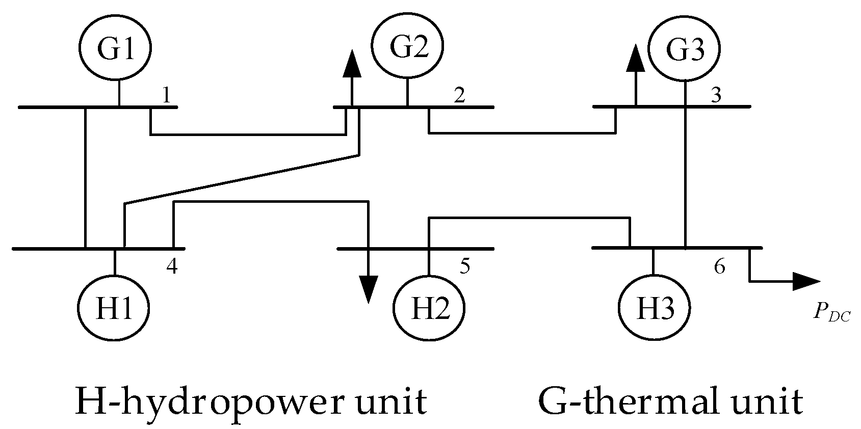
4.1. The Test System

To verify the effectiveness of the proposed hydropower generation and export coordinated optimal operation model, this paper conducts case studies based on a modified 6-bus power system. All optimization models are solved using Gurobi 11.0.

As shown in Figure 2, the cascade hydropower system consists of three hydropower stations, H1 to H3, which are located along the same river and arranged sequentially from upstream to downstream. Water naturally flows from the most upstream station to the most downstream one, forming a typical series connection. These hydropower units usually supply the base load, as well as participate in load following, frequency regulation, and reserve provision. Their fast-ramping ability enables them to effectively respond to load fluctuations. The minimum startup time for all three hydropower units is set as 1 h. The ramping rates are set as 3.67 MW/min for H1, 3.17 MW/min for H2, and 2.83 MW/min for H3. G1, G2, and G3 are three thermal units that primarily perform peak regulation, reserve provision, and system stability enhancement. They could be coordinated with hydropower units to ensure reliable load supply under complex hydrological conditions. The minimum ON time for all three thermal units are set as 8 h, and the minimum OFF time are set as 4 h. The ramp rates are set as 2.5 MW/min for G1, 1.25 MW/min for G2, and 2.08 MW/min for G3.

The power system includes six buses and seven transmission lines, with bus 6 serving as the power export node connecting the external power grid. The scheduling time horizon is set as 24 h with hourly time intervals.

To analyze the impact of dynamic water flow delay and hydropower export on system generation cost and water spillage, six cases are designed for comparative analysis:

Case 1: High-water period without dynamic water flow delay; Hydropower export is set as a fixed value.

Case 2: Based on Case 1, dynamic water flow delay is considered.

Case 3: Based on Case 2, hydropower export is further optimized.

Case 4: Normal-water period without dynamic water flow delay; Hydropower export is set as a fixed value;

Case 5: Based on Case 4, dynamic water flow delay is considered.

Case 6: Based on Case 5, hydropower export is further optimized.

For each case, the optimization model is to minimize the total operation cost, namely (1) as defined in Section 2.1, and is subject to constraints including hydraulic coupling constraints (2) and (3), water flow delay constraints (6)–(8), line flow constraints (24)–(27), and export regulation constraints (28)–(33). The optimization models are solved using commercial solver Gurobi.

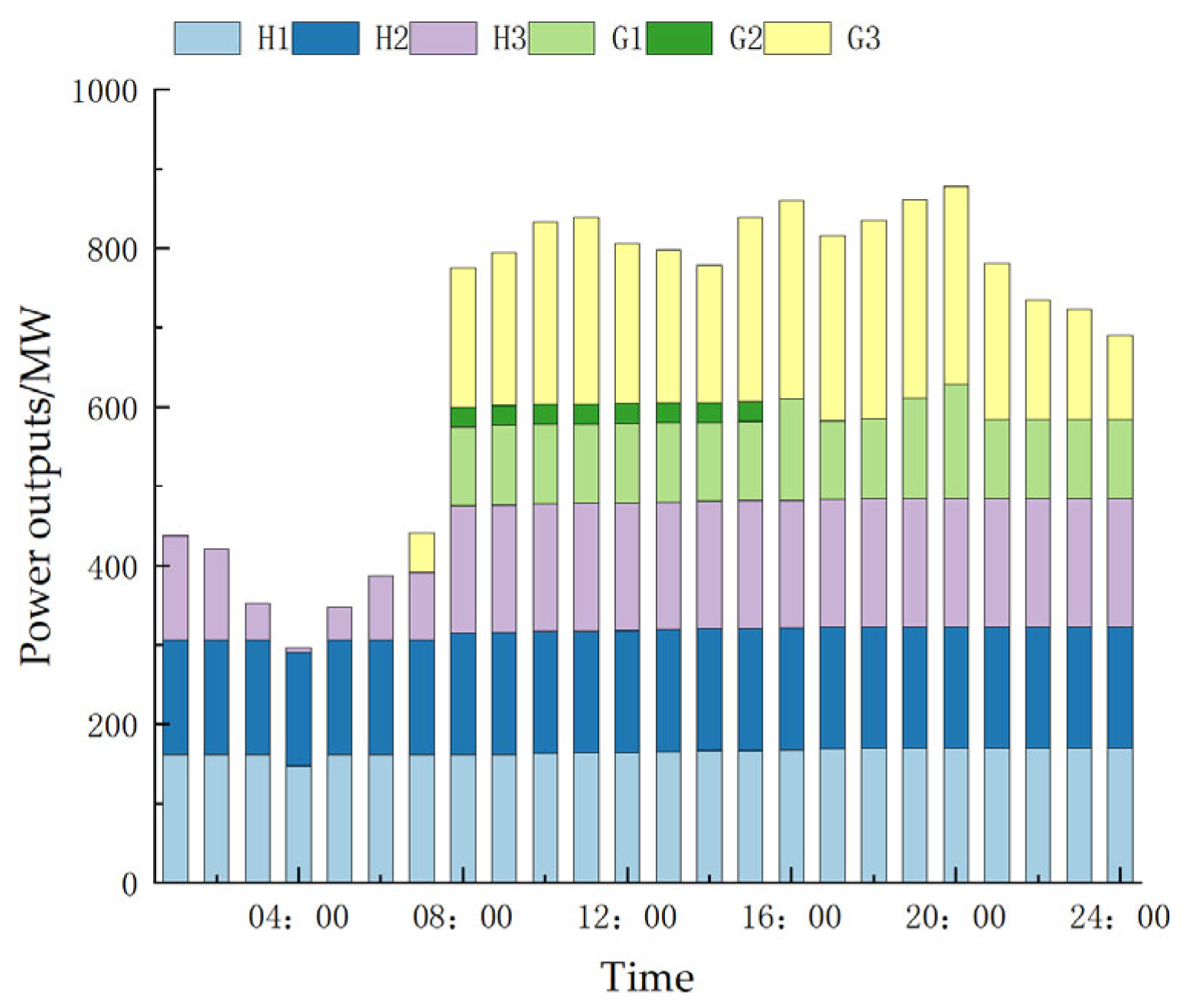
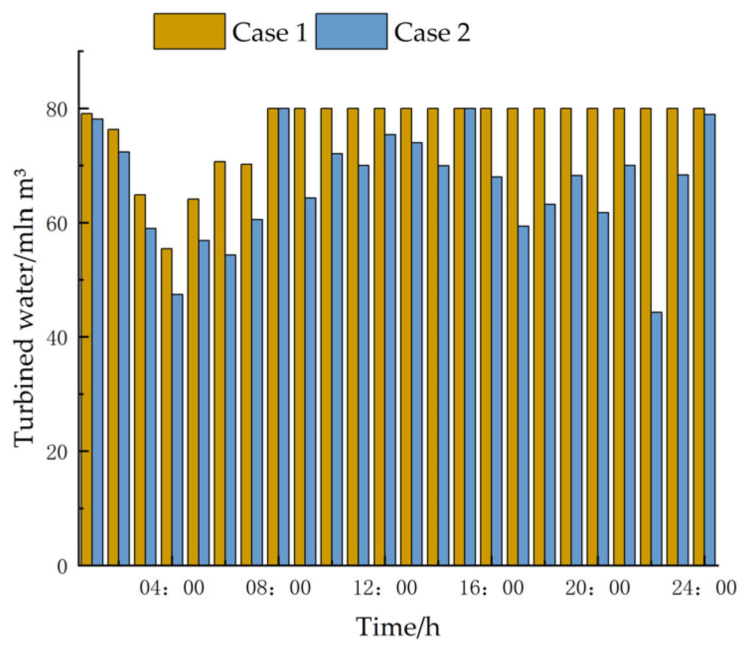
4.2. Result Analysis

Table 1. Cost comparison of different case studies.

Case	Total Cost ($)	Operating Cost ($)	Water Spillage Volume (mln m3)	Thermal Unit ON Time (h)
1	1,200,895	26,814	2739.53	43
2	300,078	32,733	623.81	36
3	298,746	31,422	623.75	35

presents a comparison of the total cost and operating cost for Case 1 to 3. The dispatch results of all unit in Case 1, including thermal and hydropower units, are shown in Figure 3. As hydropower units have no generation cost, they are prioritized over thermal units. During the time period from 00:00 to 06:00, due to low nighttime load and export demand, the hydropower units are sufficient to support the base load alone, and all thermal units are OFF. From 07:00 to 08:00, as the load increases, thermal unit G3, which has the lowest generation cost among the thermal units, begins to increase its output. After 08:00, the export power reaches 400 MW, and all thermal units are ON. During the high-load and high-export period from 08:00 to 15:00, G2, which has the highest generation cost, becomes ON serving as the peaking unit. After 15:00, G2 is shut down, and the outputs of G1 and G3 are increased to compensate for the power gap. After 21:00, as both load and export power decrease, the outputs of G1 and G3 are accordingly reduced. However, due to the low load demand during period 00:00 to 07:00, hydropower resources are not fully utilized, resulting in a significant amount of water spillage, which in turn increases the overall system cost.

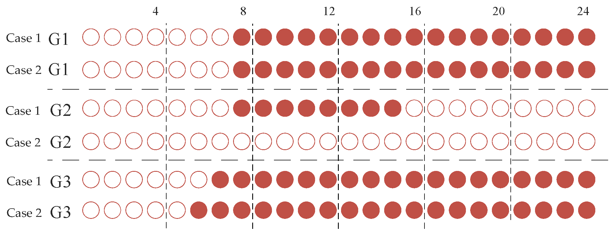
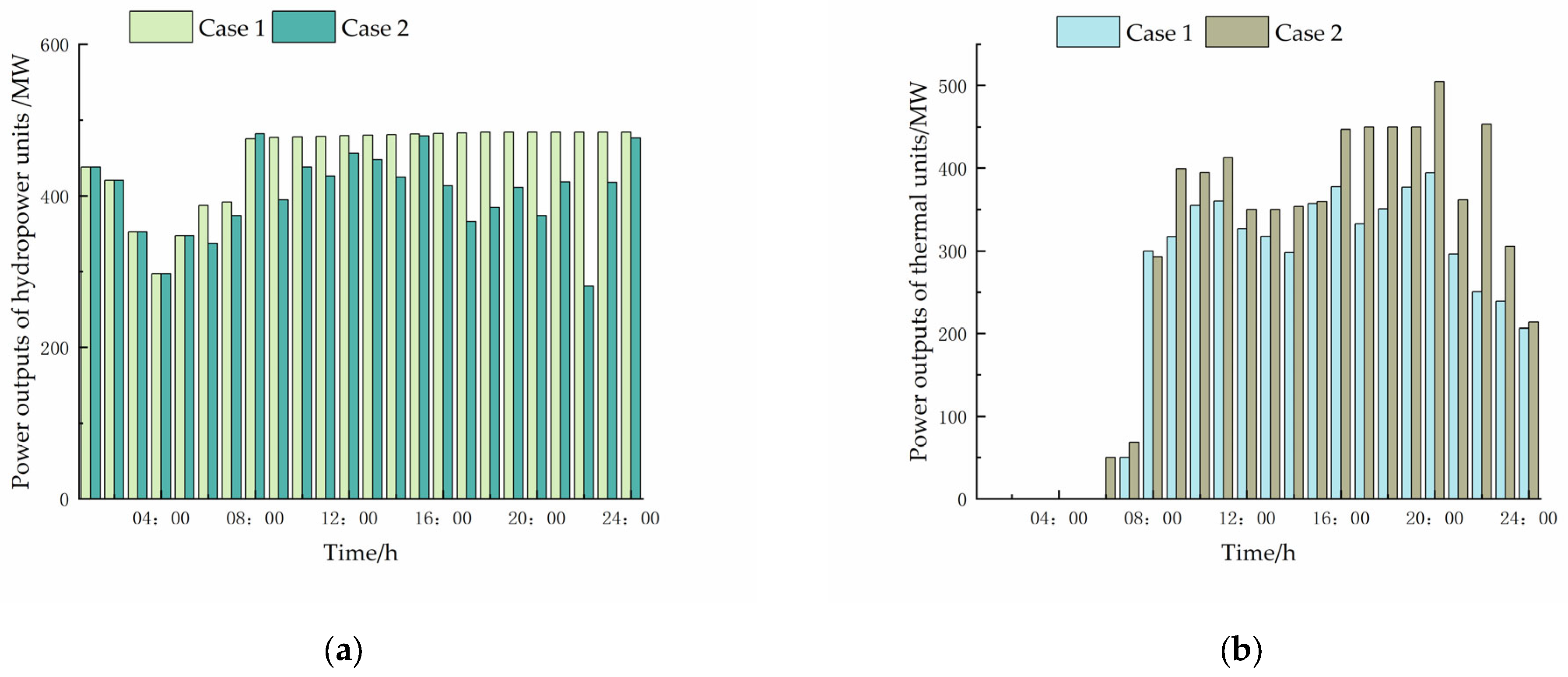
4.2.1. Comparison of Cases 1 and 2

In Case 2, dynamic water flow delay is considered based on the setup of Case 1. Compared to Case 1, accurately considering water flow delay in Case 2 significantly reduces the water spillage from 2739.53 mln m³ to 623 mln m³, leading to a substantial decrease in water spillage penalty costs. However, the total turbined water decreases, as illustrated in Figure 4. This is because, as water flow delay is considered, the water discharge from upstream stations is not immediately available to the downstream stations and additionally, part of the water is retained in the river segment as channel storage. As a result, when both upstream and downstream units need to increase their output simultaneously, the available water may be insufficient for the downstream hydropower stations. In this case, thermal units increase their output to compensate for the power gap with a higher generation cost.

The ON/OFF statuses of thermal units are shown in Figure 5, and the hourly outputs of are shown in Figure 6. From 00:00 to 05:00, all thermal units are OFF. Although turbined water fluctuates slightly during this period, the hydropower units are sufficient to meet the load. After 06:00, a more significant fluctuation of turbined water occurs, prompting thermal unit G3, which has the lowest generation cost, to start one hour earlier than in Case 1 for compensating for the power gap caused by reduced turbined water. Compared to Case 1, G2, the unit with the highest generation cost, remains OFF throughout the scheduling time horizon. Therefore, G1 and G3 noticeably increase their output to fill the power gap of G2 and decreased hydropower generation. It can be seen, considering water flow delay significantly impacts both the amount of water spillage and the associated penalty costs, validating the importance of accurately capturing water flow delays. In fact, accurately capturing water flow delays could contribute to providing more reliable dispatch results in practical applications, thereby enhancing the economic efficiency and operational feasibility of the system.

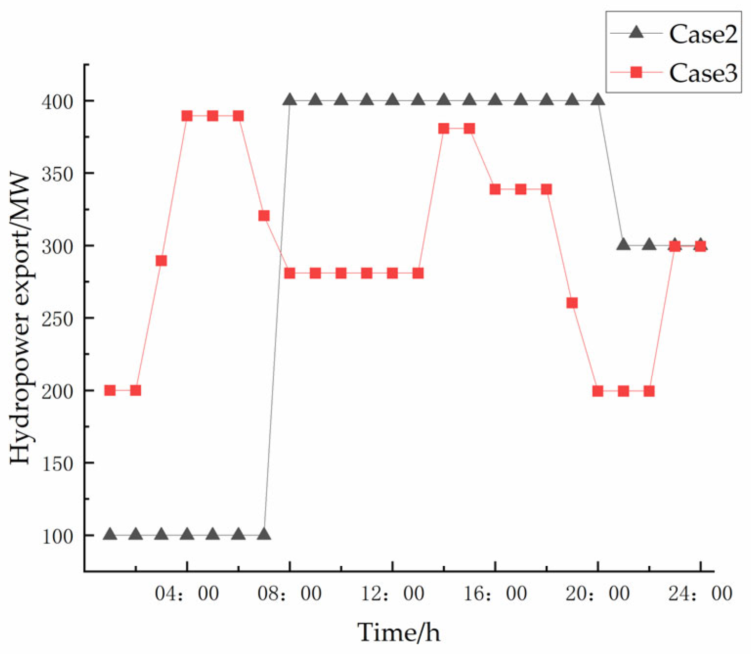
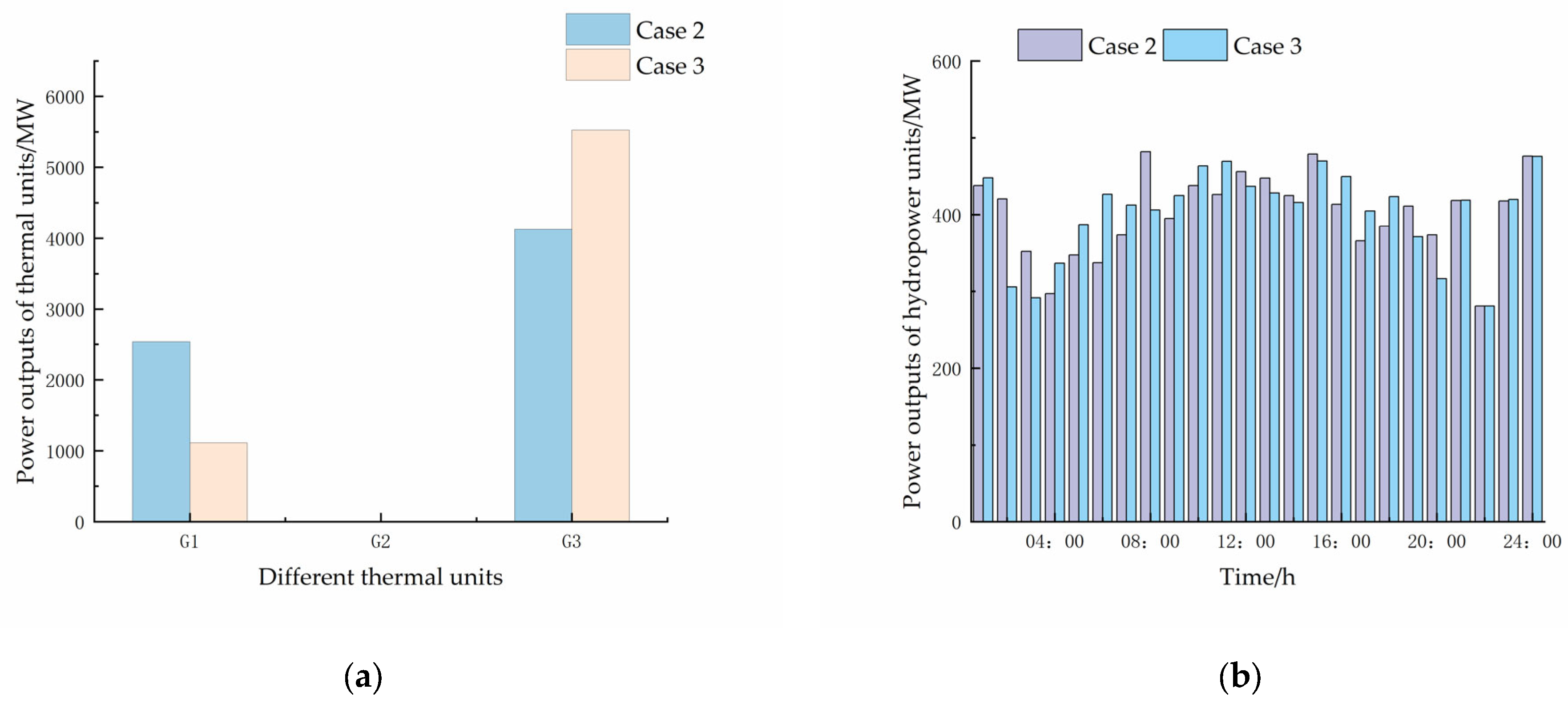
4.2.2. Comparison of Cases 2 and 3

Case 3 is built based on Case 2 by enabling optimizing hydropower export. The fixed export power and optimized export power are compared in Figure 7. In Figure 7, the black curve indicates the day-ahead forecast of hydropower export, representing the traditional power export scheduling. By contrast, the red curve illustrates the optimized hydropower export, which is constrained by (28) to (33). Under the traditional fixed-power export mode, the power export typically increases during peak load periods and decreases during off-peak periods. To improve overall system economic efficiency while keeping the total daily exported energy unchanged, which is set as 7100 MW/h, in Case 3, the power export is optimized.

After optimization, the power export increases during low-demand periods, e.g., nighttime, to fully utilize hydropower surplus and avoid hydraulic resource wastage. Moreover, the power export is reduced during high-demand periods (08:00–20:00) to alleviate pressure on supplying local load and avoid dispatching high-cost thermal units. As shown in Figure 6, the optimized power export in Case 3 increases during off-peak hours and decreases from 08:00 to 20:00.

Figure 8 compares the hourly and total power generation of thermal units in Cases 2 and Case 3. Compared with Case 2, Case 3 achieves a lower total power generation from thermal units. The power generation from G3, the most cost-effective thermal unit, increases significantly, while the output from G1, which has a higher generation cost, decreases noticeably. The most expensive unit, G2, remains OFF throughout the scheduling time horizon. As shown in Figure 8b, the hydropower output in Case 3 is generally higher than that in Case 2, particularly during 04:00–07:00, when the demand is relatively low. With increased power export during this period, more hydropower is generated, improving the utilization of hydraulic resources. It can be seen that by optimizing the power export especially during periods of hydropower surplus, the total system operating cost can be significantly reduced, highlighting the critical value of coordination hydropower generation and export.

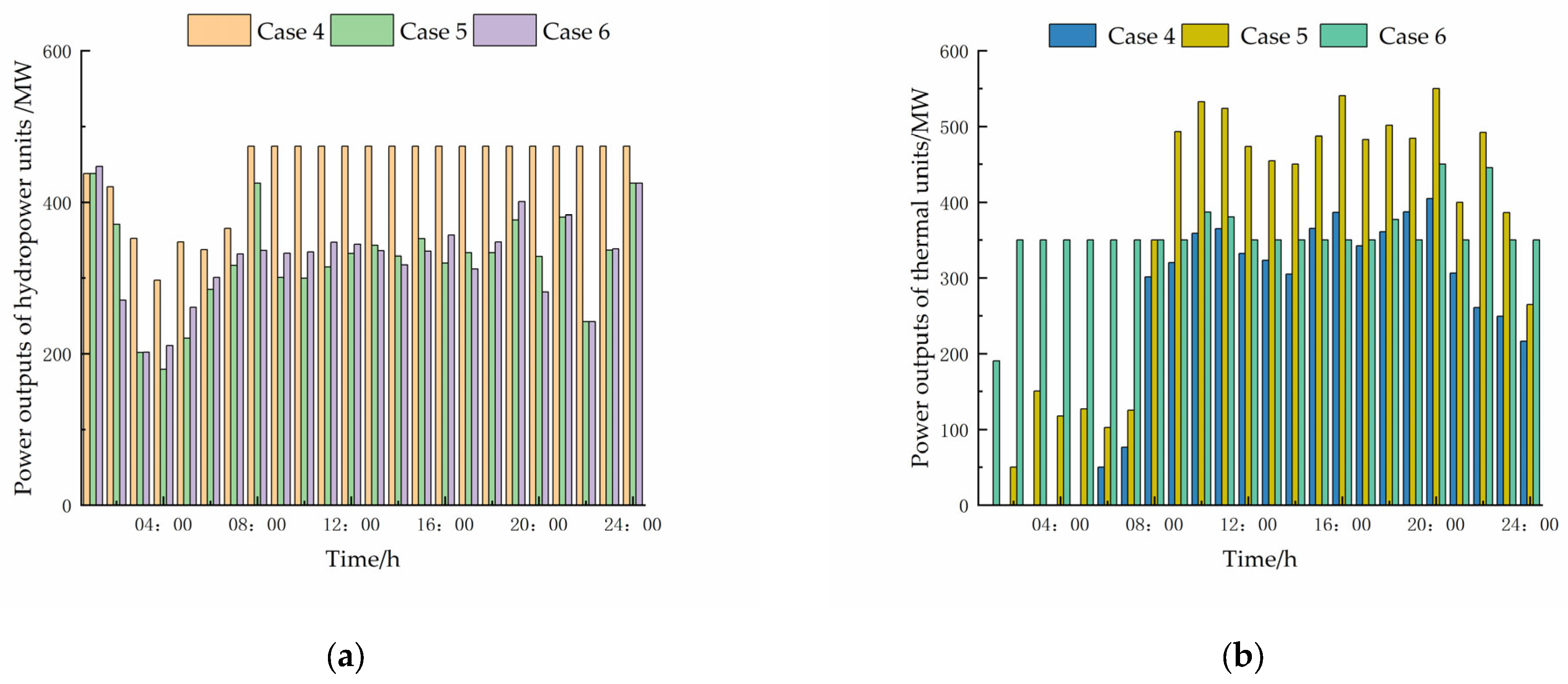
4.2.3. Comparison of Cases 4 and 6

Cases 4, 5, and 6 are all under normal water period conditions, focusing on the impacts of dynamic water flow delay and hydropower power export optimization under varying flow conditions.

Table 2. Result comparison of Cases 4 to 6.

Case	Total Cost ($)	Operating Cost ($)	Water Spillage Volume (mln m3)	Thermal Unit ON Time (h)
4	598,552	27,483	1332.49	41
5	138,347	43,163	222.10	40
6	136,141	40,984	222.03	47

presents a comparison of the results in terms of total cost and operating cost for Cases 4 to 6.

Compared to Case 4, the water spillage in Case 5 is reduced from 1332.49 mln m³ to 222 mln m³. Even though the natural inflow to the hydropower stations during the normal water period is smaller than in the high-water period, the water spillage is still greatly reduced. As shown in Figure 9, during most time periods, the hydropower output in Case 4 is significantly higher than in Case 5. This is mainly because, in Case 4, dynamic water flow delay is ignored, allowing immediate availability of inflows from upstream for power generation. In contrast, after incorporating water flow delay in Case 5, the available water for power generation during certain periods is reduced, thereby lowering the output of hydropower units. The resulting power gap is ultimately covered by thermal units.

Case 6 is built upon Case 5 by considering the optimization of power export. As shown in Table 2, both the operating cost and the total cost are reduced after considering the optimization of power export. Figure 9 indicates that, compared to Case 5, hydropower output generally increases at most time periods. However, between 01:00 and 06:00, due to insufficient hydropower output to fully meet the load demand, thermal units are dispatched to fill the power gap. In the remaining periods, the power output of thermal units is significantly reduced. The operating cost of Case 6 is 5.05% lower than that of Case 5.

Based on the above cases, it can be concluded that even under relatively low water inflow conditions during the normal flow period, the proposed model can still accurately simulate operational characteristics of cascade hydropower stations, demonstrating strong adaptability.

In all the above cases, Cases 1 to 3 are set under high water period conditions, while Cases 4 to 6 correspond to normal water period conditions. The primary difference between the two hydrological periods lies in the volume of natural inflow, with the normal water period receiving approximately 43% less inflow compared to the high-water period. The comparison in Table 1 and Table 2 shows that under the same scheduling method and case settings, the reduction in natural inflow during the normal water period significantly increases operational costs, despite a decline in total costs due to the substantial reduction in water spillage penalty costs.

Specifically, under the same case settings, the operational costs in cases of normal water period are consistently higher than those in the high-water period counterparts. For instance, both considering dynamic water flow delay, the operational cost of Case 5 (USD 43,163) is 31.86% higher than that of Case 2 (USD 32,733); both considering hydropower export optimization, the operational cost of Case 6 (USD 40,984) is 30.43% higher than that of Case 3 (USD 31,422). Even without considering dynamic water flow delay and hydropower export optimization, the operational cost of Case 4 (USD 27,483) exceeds that of Case 1 (USD 26,814), indicating that water scarcity directly increases the cost of system operation.

Furthermore, in cases of normal water period, considering dynamic water flow delay could lead to a greater increase in operational cost than in the high-water period. For example, a 57.05% increase occurs from Case 4 to 5, compared to only 22.07% from Case 1 to 2, reflecting that water scarcity significantly amplifies the sensitivity of operational cost to scheduling.

5. Conclusions

To address the oversimplification in existing models regarding river flow evolution and the lack of coordination between hydropower generation and export, this paper proposes a coordinated optimal operation model that integrates dynamic water flow delay to minimize the system operating cost. The case study verifies the effectiveness of the proposed model in improving hydraulic resource utilization, reducing water spillage, and optimizing thermal unit operation.

• The refined modeling of dynamic water flow delay can capture the evolution process, and thereby improving the coordination efficiency, accurately quantifying the amount of spilled water, and decreasing the startup frequency of high-cost thermal units.
• By jointly optimizing the hydropower export, the operating cost of the system can be effectively reduced and the flexibility of hydropower stations can be well exploited.
• Even during normal water flow periods, the proposed hydropower generation and export coordinated optimal operation model can still achieve low water spillage and slight increase in the operating cost, indicating that the proposed mode could maintain high performance and realize benefits under various hydrological conditions.
• For environmental and social benefits, by reducing water spillage and optimizing hydro-thermal coordination, this proposed method could help protect the river ecosystem by maintaining a more stable ecological base flow, lower the overall carbon emissions of the system by reducing the operation of high-cost, high-emission thermal power units, and enhance the stability and reliability of power supply that indirectly supports residential electricity consumption and industrial production.

The refined segmented Muskingum method improves the modeling accuracy of water delay but would significantly increase the computation burden with complex river networks. Additionally, accurately obtaining hydraulic parameters for a complex river network is difficult, and parameter uncertainty could affect model accuracy. Future work will focus on improving computational efficiency and adaptability by developing efficient solving algorithms and exploring hybrid modeling approaches (e.g., combining data-driven and physical models) to better handle parameter uncertainty and complex river hydraulics.

References

1. Yan, T.; Guo, S.; Sun, H. Complementary Scheduling of Cascade Hydropower Stations and Photovoltaic Power Considering Daily Regulating Hydropower Stations. In Proceedings of the 2024 IEEE PES 16th Asia-Pacific Power and Energy Engineering Conference (APPEEC), Nanjing, China, 25 October 2024; IEEE: New York, NY, USA, 2024; pp. 1–5. [Google Scholar]
2. Wang, Y.; Shi, P.; Zeng, Z.; Li, X.; Zhou, B. Coordinated Operation of PV and Cascaded Hydropower Considering the Power Grid Security Constraints. In Proceedings of the 2021 International Conference on Power System Technology (POWERCON), Haikou, China, 8 December 2021; IEEE: New York, NY, USA, 2021; pp. 1035–1039. [Google Scholar]
3. Liu, Y.; Zhou, J.; Chang, C.; Lu, P.; Wang, C.; Tayyab, M. Short-Term Joint Optimization of Cascade Hydropower Stations on Daily Power Load Curve. In Proceedings of the 2016 IEEE International Conference on Knowledge Engineering and Applications (ICKEA), Singapore, Singapore, 28–30 September 2016; IEEE: New York, NY, USA, 2016; pp. 236–240. [Google Scholar]
4. Zhu, Y.; Zhou, Y.; Xu, C.-Y.; Chang, F.-J. Optimizing Complementary Operation of Mega Cascade Reservoirs for Boosting Hydropower Sustainability. Sustain. Energy Technol. Assess. 2024, 64, 103719. [Google Scholar] [CrossRef]
5. Wu, Y.; Liao, S.; Liu, B.; Cheng, C.; Zhao, H.; Fang, Z.; Lu, J. Short-Term Load Distribution Model for Cascade Giant Hydropower Stations with Complex Hydraulic and Electrical Connections. Renew. Energy 2024, 232, 121067. [Google Scholar] [CrossRef]
6. Chen, X.; Pan, X.; Sun, X. Evaluation and Decision of Joint Dispatch Schemes for Cascade Hydropower Stations Based on the Prospect Theory. In Proceedings of the 2020 12th IEEE PES Asia-Pacific Power and Energy Engineering Conference (APPEEC), Nanjing, China, 20–23 September 2020; IEEE: New York, NY, USA, 2020; pp. 1–5. [Google Scholar]
7. Ge, X.; Zhang, L.; Shu, J.; Xu, N. Short-Term Hydropower Optimal Scheduling Considering the Optimization of Water Time Delay. Electr. Power Syst. Res. 2014, 110, 188–197. [Google Scholar] [CrossRef]
8. Yuan, W.; Zhang, S.; Su, C.; Wu, Y.; Yan, D.; Wu, Z. Optimal Scheduling of Cascade Hydropower Plants in a Portfolio Electricity Market Considering the Dynamic Water Delay. Energy 2022, 252, 124025. [Google Scholar] [CrossRef]
9. Xu, B.; Zhong, P.; Zhang, M.; Zhang, J. Short Term Optimization of Cascade Reservoirs Operation Considering Flow Routing. In Proceedings of the 2012 Asia-Pacific Power and Energy Engineering Conference, Shanghai, China, 27–29 March 2012; IEEE: New York, NY, USA, 2012; pp. 1–4. [Google Scholar]
10. Souza, T.M. An Accurate Representation of Water Delay Times for Cascaded Reservoirs in Hydro Scheduling Problems. In Proceedings of the 2012 IEEE Power and Energy Society General Meeting, San Diego, CA, USA, 22–26 July 2012; IEEE: New York, NY, USA, 2012; pp. 1–7. [Google Scholar]
11. Weiss, O.; Pareschi, G.; Schwery, O.; Bolla, M.; Georges, G.; Boulouchos, K. Long-Term Scheduling Model of Swiss Hydropower. In Proceedings of the 2019 16th International Conference on the European Energy Market (EEM), Ljubljana, Slovenia, 18–20 September 2019; IEEE: New York, NY, USA, 2019; pp. 1–5. [Google Scholar]
12. Liao, S.; Liu, H.; Liu, Z.; Liu, B.; Li, G.; Li, S. Medium-Term Peak Shaving Operation of Cascade Hydropower Plants Considering Water Delay Time. Renew. Energy 2021, 179, 406–417. [Google Scholar] [CrossRef]
13. Wang, W.; Tian, W.; Xu, D.; Chau, K.; Ma, Q.; Liu, C. Muskingum Models’ Development and Their Parameter Estimation: A State-of-the-Art Review. Water Resour. Manag. 2023, 37, 3129–3150. [Google Scholar] [CrossRef]
14. Gill, M.A. Flood Routing by the Muskingum Method. J. Hydrol. 1978, 36, 353–363. [Google Scholar] [CrossRef]
15. Mohsenabadi, S.K. Flood Routing in D-Shape Tunnels through Multilinear Muskingum Method. KSCE J. Civ. Eng. 2025, 29, 100031. [Google Scholar] [CrossRef]
16. Si-min, Q.; Wei-min, B.; Peng, S.; Zhongbo, Y.; Peng, J. Water-Stage Forecasting in a Multitributary Tidal River Using a Bidirectional Muskingum Method. J. Hydrol. Eng. 2009, 14, 1299–1308. [Google Scholar] [CrossRef]
17. Zhang, W.; Liu, P.; Chen, X.; Wang, L.; Ai, X.; Feng, M.; Liu, D.; Liu, Y. Optimal Operation of Multi-Reservoir Systems Considering Time-Lags of Flood Routing. Water Resour. Manag. 2016, 30, 523–540. [Google Scholar] [CrossRef]
18. Sosnin, P. A Scientifically Experimental Approach to the Simulation of Designer Activity in the Conceptual Designing of Software Intensive Systems. IEEE Access 2013, 1, 488–504. [Google Scholar] [CrossRef]
19. Liao, S.; Xiong, J.; Liu, B.; Cheng, C.; Zhou, B.; Wu, Y. MILP Model for Short-Term Peak Shaving of Multi-Grids Using Cascade Hydropower Considering Discrete HVDC Constraints. Renew. Energy 2024, 235, 121341. [Google Scholar] [CrossRef]
20. Su, C.; Cheng, C.; Wang, P.; Shen, J. Optimization Model for the Short-Term Operation of Hydropower Plants Transmitting Power to Multiple Power Grids via HVDC Transmission Lines. IEEE Access 2019, 7, 139236–139248. [Google Scholar] [CrossRef]
21. Shen, J.; Cheng, C.; Zhang, J.; Lu, J. Peak Operation of Cascaded Hydropower Plants Serving Multiple Provinces. Energies 2015, 8, 11295–11314. [Google Scholar] [CrossRef]
22. Liu, B.; Liu, T.; Liao, S.; Wang, H.; Jin, X. Short-Term Operation of Cascade Hydropower System Sharing Flexibility via High Voltage Direct Current Lines for Multiple Grids Peak Shaving. Renew. Energy 2023, 213, 11–29. [Google Scholar] [CrossRef]
23. Feng, Y.; Zheng, R.; Ma, D.; Huang, X. Associating Reservoir Operations with 2D Inundation Risk and Climate Uncertainty. Water Supply 2024, 24, 2598–2613. [Google Scholar] [CrossRef]
Figure 1. Piecewise linearization of hydropower conversion.
Energies 18 03917 g001
Figure 2. Modified 6-bus system.
Energies 18 03917 g002
Figure 3. Power outputs of all units at different time intervals.
Energies 18 03917 g003
Figure 4. Comparison of turbined water in Case 1 and Case 2.
Energies 18 03917 g004
Figure 5. ON and OFF statuses of thermal units in Case 1 and Case 2.
Energies 18 03917 g005
Figure 6. Comparison of power outputs in Case 1 and Case 2. (a) Power outputs of hydropower units at different time intervals. (b) Power outputs of thermal units at different time intervals.
Energies 18 03917 g006
Figure 7. Hydropower export in Case 2 and Case 3.
Energies 18 03917 g007
Figure 8. Power outputs of all units at different time intervals in Case 2 and Case 3: (a) thermal power units’ aggregate output (b) power outputs of hydropower units at different time intervals.
Energies 18 03917 g008
Figure 9. Comparison of unit outputs in Cases 4 to 6: (a) comparison of hydropower unit outputs (b) comparison of thermal unit outputs.
Energies 18 03917 g009