A Numerical Investigation of the Flame Characteristics of a CH₄/NH₃ Blend Under Different Swirl Intensity and Diffusion Models

Abstract

This study investigates the effects of diffusion modeling and swirl intensity on flow fields and NO emissions in CH₄/NH₃ non-premixed swirling flames using large eddy simulations (LESs). Simulations are performed for a 50/50 ammonia–methane blend at three global equivalence ratios of 0.77, 0.54, and 0.46 and two swirl numbers of 8 and 12, comparing the unity Lewis number (ULN) and mixture-averaged diffusion (MAD) models against the experimental data includes OH-PLIF and ON-PLIF reported in a prior study by the KAUST group. Both models produce similar flow fields, but the MAD model alters the flame structure and species distributions due to differential diffusion (DD) and limitations in its Flamelet library. Notably, the MAD library lacks unstable flame branch solutions, leading to extensive interpolation between extinction and stable branches. This results in overpredicted progress variable source terms and reactive scalars, both within and beyond the flame zone. The ULN model better reproduces experimental OH profiles and localizes NO formation near the flame front, whereas the MAD model predicts broader NO distributions due to nitrogen species diffusion. Higher swirl intensities shorten the flame and shift NO production upstream. While a low equivalence ratio provides enough air for good mixing, lower ammonia and higher NO contents in exhaust gases, respectively.

1. Introduction

The power sector forms a cornerstone of modern civilization, evolving to meet the growing global energy demand [1]. Among various energy sources, fuels remain the most energy-dense medium, capable of being burned to produce thermal energy for power generation in heat engines such as gas turbines and internal combustion engines.

Despite the advantages of fuels, their combustion generates chemical pollutants such as CO₂, CO, and NO_X, which contribute to greenhouse gas emissions and global warming. This has prompted the adoption of energy policies prioritizing carbon-neutral and carbon-free power generation to mitigate environmental impacts. In this context, hydrogen and ammonia have emerged as promising alternatives to fossil fuels. Being carbon-free species, their blends can offer a comparable performance to fossil fuels [2]. However, challenges related to their storage, transportation, and combustion processes remain significant [3].

Ammonia is a promising fuel because it can be transported and stored using existing infrastructure with minimal modifications, unlike hydrogen. Additionally, ammonia can serve as a hydrogen carrier, decomposing into hydrogen and nitrogen when needed [3]. However, ammonia faces challenges due to its low combustion performance, including a high ignition temperature (930 K) and a low laminar flame speed (0.072 m/s) [4]. To address these limitations, ammonia is often blended with hydrocarbons such as methane [5] or with hydrogen [2] to enhance its combustion characteristics.

In the industrial and power sectors, most flames are turbulent to meet power requirements while ensuring flame stability. This is often achieved using swirling combustion, where the air flow creates a recirculation zone near the burner rim. This recirculation increases the fuel’s residence time in the highly reactive zone, enhancing combustion. As a result, the swirl number plays a critical role in determining the flame characteristics [6].

The LES/FPV (large eddy simulation/Flamelet progress variable) approach is a widely adopted modeling framework for turbulent combustion due to its ability to combine detailed chemistry with the resolution of large-scale turbulent structures. In this method, combustion is represented using precomputed Flamelet libraries parameterized by variables such as the mixture fraction and a progress variable, while LES resolves the energy-containing eddies that strongly influence flame dynamics [7,8]. A major advantage of LES/FPV is its computational efficiency compared to direct numerical simulation (DNS), enabling the study of complex, realistic configurations, such as gas turbines and engines, while capturing key turbulence–chemistry interactions [9]. It also facilitates a direct comparison with experiments by allowing the computation of filtered scalar quantities like LIF and Rayleigh signals [10]. However, the approach relies on assumptions such as the Flamelet regime being valid and the use of presumed probability density functions (PDFs) to reconstruct subgrid scalar statistics, which may reduce accuracy in regimes with ignition, extinction, or strong stratification [11]. Despite these limitations, LES/FPV remains a popular tool due to its balance between physical fidelity and computational feasibility, making it attractive for both academic and industrial combustion research [12].

The LES/FPV approach is used in the previous works to investigate the flame characteristics. For example, the flame structure of a piloted partially premixed dimethyl ether (DME) was investigated using LES/FPV. The numerical results were compared with experimental data, including temperature and species measurements (Raman/Rayleigh, LIF) and velocity fields (PIV), which showed good agreement [13]. The diffusion models of the Flamelet libraries were investigated for a turbulent non-premixed oxy-fuel flame using experimental data and LES simulations [14]. A species-weighted Flamelet model accounting for DD was developed and applied in the LES of oxy-fuel flames, showing improved predictions of flame structure and extinction behavior compared to traditional unity and species-constant Lewis number models [15]. LESs were performed for turbulent CH₄/H₂ flames with and without fuel stratification, using Flamelet libraries based on ULN and MAD models. Two approaches were used to access the libraries: one solving species transport equations and the other solving trajectory variables directly. The results showed that accounting for heat loss and using the trajectory-based approach improved agreement with experiments, and that DD effects played a key role in downstream flame behavior [16]. Building on these studies, the present work incorporates heat loss and mixture fraction variance in the Flamelet library to model turbulent non-premixed flames, and systematically compares two diffusion models: ULN and MAD.

Recent studies have advanced the understanding of ammonia and hydrogen combustion. Su et al. [17] analyzed chemiluminescence in NH₃–CH₄ laminar flames and identified CH*/NH₂* as a potential marker for ammonia content, but their work was limited to laminar conditions. Osetrov and Haas [18] developed a Wiebe-based model for hydrogen combustion in spark-ignition engines, focusing on mixture stratification and ignition control, though their study did not consider ammonia or swirling diffusion flames. Lan et al. [19] showed that hydrogen enrichment in natural gas flames reduces CO and CO₂ emissions but increases NO_x, emphasizing trade-offs in fuel composition; however, turbulence and diffusion modeling were not the focus. Liu et al. [20] linked pressure fluctuations in swirl combustors to heat release, swirl, and flame detachment using EMD, FFT, and POD, but without exploring diffusion effects. Wu et al. [21] showed the efficiency and emission benefits of diesel/ammonia dual-fuel engines but did not investigate the turbulent flame structure or DD effects. Wang et al. [22] investigated the DD effects in transcritical LO₂/CH₄ flames using large-eddy simulations and the FPV model, where Flamelets were solved in mixture fraction space with both unity and non-unity Lewis numbers. In the present study, DD is treated differently by solving the Flamelet equations in a physical space using the MAD model, which account for the different values of the Lewis number for the same species at different conditions, while a constant Lewis number considers only one value for the Lewis number per species regardless of its different conditions. Obando Vega et al. [23] focused on modeling the subgrid-scale effects in the LES of turbulent non-premixed flames using filtered tabulated chemistry to capture flame front wrinkling and strain-rate influences, while the DD was also considered by solving the Flamelet equation using a constant Lewis number in mixture fraction space.

To address the limitations highlighted in previous studies, such as the lack of turbulence, swirl effects, and advanced diffusion modeling, this work investigates CH₄/NH₃ non-premixed turbulent swirling flames using high-fidelity numerical simulations. It compares two widely used diffusion models in Flamelet equations, the unity Lewis number (ULN) and mixture-averaged diffusion (MAD) approaches, solved in mixture fraction and physical space, respectively. Their predictions of key scalar fields, including OH and NO, are validated against experimental data to evaluate each model’s ability to capture the flame structure properly. The combined impact of swirl intensity and diffusion treatment on flame structure is further analyzed using Flamelet libraries. By benchmarking against experimental results from [6], the study provides new insights into the predictive performance of diffusion models under realistic turbulent combustion conditions.

2. Numerical Methods and Modeling

This study investigates two sets of simulation cases. The first set employs a ULN Flamelet library, assuming equal diffusivity for all species, while the second set incorporates DD effects using a mixture-averaged diffusion (MAD) model. The key configurations and parameters for each case are summarized in

Table 1. Investigation program.

	Case 1	Case 2	Case 3	Case 4
ULN	$S_g=8$	$S_g=8$	$S_g=8$	$S_g=12$
	$\varphi =0.46$	$\varphi =0.54$	$\varphi =0.77$	$\varphi =0.54$
MAD	$S_g=8$	$S_g=8$	$S_g=8$	$S_g=12$
	$\varphi =0.46$	$\varphi =0.54$	$\varphi =0.77$	$\varphi =0.54$

, where $S_g$ denotes the swirl number defined in [6] and $\varphi$ is the global equivalence ratio. The selected values are based on the experimental cases reported in [6], where $\varphi$ = 0.54 produced the highest NO emissions at $X_{NH3}=0.5$ and $S_g=8$, while the other two equivalence ratios, although still lean, produced lower NO levels. These points were selected to explore the sensitivity of NO formation to slight variations in fuel–air equivalence under lean conditions.

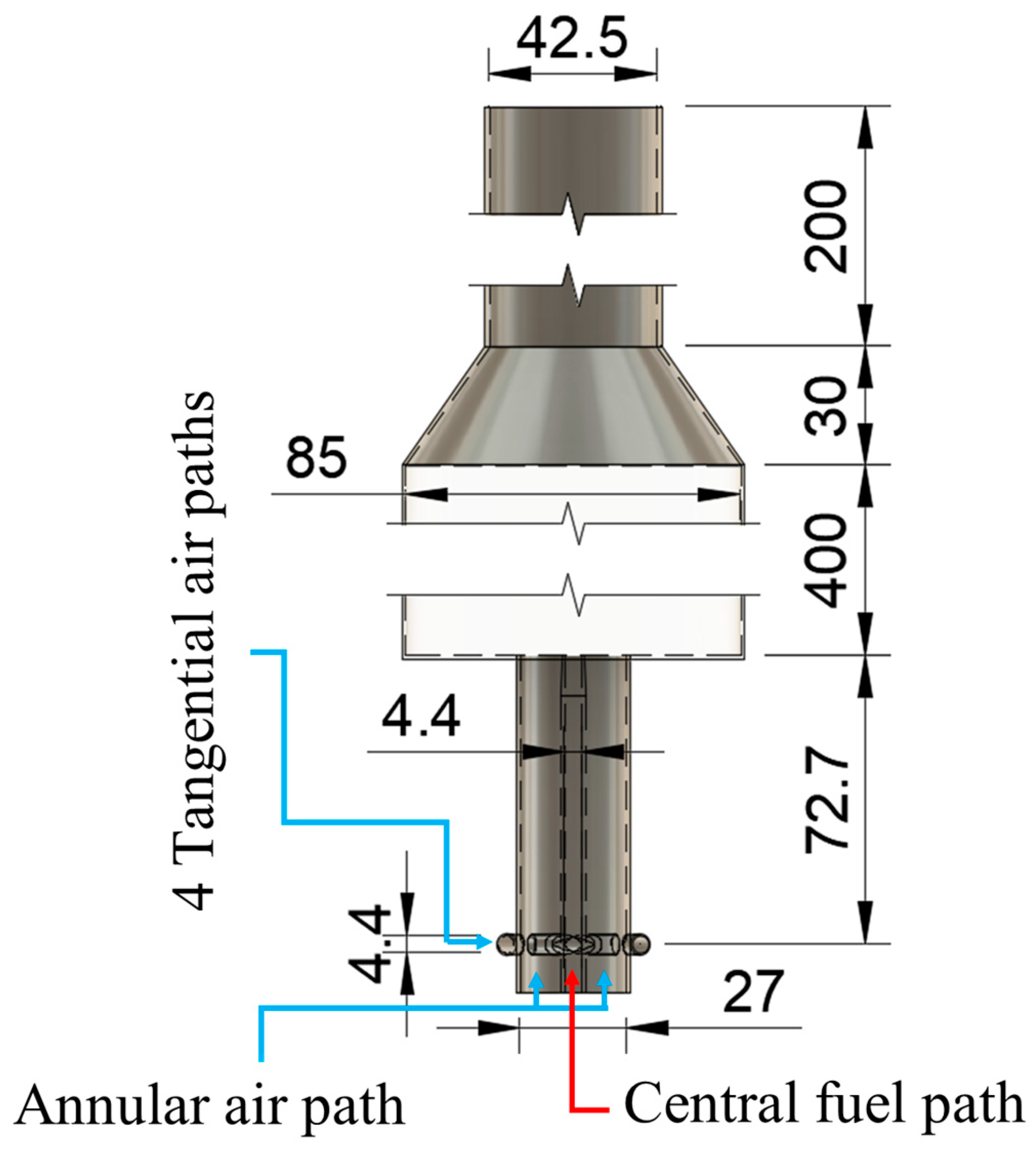
2.1. Geometry and Grid Configurations

The LESs are conducted on the same burner and combustor configuration mentioned in [6]. Figure 1 shows the rendered view of the metallic burner fixed with the fiber glass combustor: the burner consists of two concentric pipes, the central pipe supplies fuel to the combustion chamber at constant velocity equal to 13 m/s for all investigated cases, while the annular pipe has five inlets, one is axial and four are tangential, the flow rates of air inlets are manipulated to achieve different global equivalence ratios and swirl numbers. The swirl number is calculated using $S_g={\displaystyle \frac{\pi r_o{d}_a}{2A_t}}\times {\left({\displaystyle \frac{{\dot{m}}_{air,t}}{{\dot{m}}_{air,t}+{\dot{m}}_{air,a}}}\right)}^2$, where $r_o=d_a-d_f$, $d_a$ is the annular large diameter, i.e., 27 mm and $d_f$ is the fuel pipe inner diameter, i.e., 4.4 mm, $A_t$ is the cross sectional area of all 4 tangential air inlets, while ${\dot{m}}_{air,t}$ and ${\dot{m}}_{air,a}$ are the total tangential and axial air mass flow rates, respectively. Based on this design, the structured grid is created.

2.2. Governing Equations

The governing equations in this LES non-adiabatic Flamelet generated manifold (NA-FGM) study are solved by front flow red (FFR) solver, they include the density weighted averaged conservation equations for mass, momentum, enthalpy $\tilde{h}$, NO mass fraction $\widetilde{Y_{NO}}$, mixture fraction $\tilde{Z}$, and progress variable $\tilde{C}$ as in Equations (1)–(6).

$${\displaystyle \frac{\partial \overline{\rho }}{\partial t}}+\nabla \cdot \left(\overline{\rho }\tilde{\mathit{u}}\right)=0$$

(1)

$${\displaystyle \frac{\partial \overline{\rho }\tilde{\mathit{u}}}{\partial t}}+\nabla \cdot \left(\overline{\rho }\tilde{\mathit{u}}\tilde{\mathit{u}}\right)=-\nabla \overline{\mathrm{P}}+\nabla \cdot \overline{\sigma }+\nabla \cdot \tau$$

(2)

$${\displaystyle \frac{\partial \overline{\rho }\tilde{h}}{\partial t}}+\nabla \cdot \left(\overline{\rho }\tilde{\mathit{u}}\tilde{h}\right)=\nabla \cdot \left(\overline{\rho }\widetilde{D_h}\nabla \tilde{h}\right)+\nabla {\cdot q}_h+Q_{rad}$$

(3)

$${\displaystyle \frac{\partial \overline{\rho }\widetilde{Y_{NO}}}{\partial t}}+\nabla \cdot \left(\overline{\rho }\tilde{\mathit{u}}\widetilde{Y_{NO}}\right)=\nabla \cdot \left(\overline{\rho }\widetilde{D_{Y_{NO}}}\nabla \widetilde{Y_{NO}}\right)+\nabla \cdot q_{Y_{NO}}+{\tilde{\dot{\omega }}}_{Y_{NO}}$$

(4)

$${\displaystyle \frac{\partial \overline{\rho }\tilde{Z}}{\partial t}}+\nabla \cdot \left(\overline{\rho }\tilde{\mathit{u}}\tilde{Z}\right)=\nabla \cdot \left(\overline{\rho }\widetilde{D_Z}\nabla \tilde{Z}\right)+\nabla \cdot q_Z$$

(5)

$${\displaystyle \frac{\partial \overline{\rho }\tilde{C}}{\partial t}}+\nabla \cdot \left(\overline{\rho }\tilde{\mathit{u}}\tilde{C}\right)=\nabla \cdot \left(\overline{\rho }\widetilde{D_C}\nabla \tilde{C}\right)+\nabla \cdot q_C+{\tilde{\dot{\omega }}}_C$$

(6)

where $\tau$ is the subgrid stress derived from the tubulence model, P is the pressure, $q_{\varphi }$ denotes the subgrid-scale terms for the scalar $\varphi$, and $\tilde{\mathit{u}}$ represents velocity in the three spatial directions, while $D_{\varphi }$ is the diffusion coefficient of the scalar $\varphi$, which is calculated using Equation (7).

$$D_{\varphi }={\displaystyle \frac{\mu }{P{r}_{\varphi }}}$$

(7)

2.3. Chemistry Modeling

This study adopts the Flamelet progress variable (FPV) approach, where equilibrium thermo-chemical states of laminar Flamelets are precomputed. The Flamelet equations in [24] are solved with the Okafor mechanism [25], which includes 59 species and 356 reactions. For non-premixed combustion, a wide range of scalar dissipation rates and stain rates up to extinction are computed for ULN and MAD models, respectively. These calculations are repeated for the different percentages of the total heat in the adiabatic case. The resulting data are then used to generate the Flamelet library, where the enthalpy difference $\Delta h$ from the adiabatic case is computed. The maximum $\Delta h$ is estimated based on the obtained Flamelet solutions. The library conditions thermo-chemical states on $\tilde{Z},\widetilde{Z^{″2} },\tilde{C},$ and $\widetilde{\mathsf{\Delta }h}$. The mixture fraction variance $\widetilde{Z^{″2} }$ follows an exponential distribution from 0 to 0.25, and the corresponding states $\tilde{\varphi }$ are computed using Equations (8)–(12) in [8].

$$\tilde{\varphi }={\int }_0^1\varphi \left(Z\right) \tilde{P}\left(Z\right)dZ$$

(8)

$$\tilde{P}={\displaystyle \frac{Z^{\alpha -1} {\left(1-Z\right)}^{\beta -1}}{\Gamma \left(\alpha \right)\Gamma \left(\beta \right)}}\mathsf{\Gamma }(\alpha +\beta )$$

(9)

$$\alpha =\tilde{Z}\gamma$$

(10)

$$\beta =\left(1-\tilde{Z}\right)\gamma$$

(11)

$$\gamma ={\displaystyle \frac{\tilde{Z}(1-\tilde{Z})}{\widetilde{Z^{″2} }}}-1\ge 0$$

(12)

Furthermore, during the LES, the total enthalpy transport equation is solved to determine the physical enthalpy at each grid point. The difference between this enthalpy and the adiabatic enthalpy from the library represents the local heat loss. This enthalpy difference is then used to retrieve the appropriate thermo-chemical state from the Flamelet library, ensuring an accurate representation of non-adiabatic effects in the simulation.

The Flamelet libraries contain equilibrium solutions of the Flamelet equations. Since NO has a larger timescale than most major species, particularly those forming the progress variable, the Flamelet model inevitably overpredicts NO [26]. To address this, the transport Equation (4) is solved while using the Flamelet library, with its source term modeled by Equation (13). This approach mitigates the high NO destruction rate, which would otherwise result from its mass fraction overprediction in equilibrium state.

$${\tilde{\dot{\omega }}}_{NO}={\tilde{\dot{\omega }}}_{NO}^{+flm}+{\tilde{Y}}_{NO}{\displaystyle \frac{{\tilde{\dot{\omega }}}_{NO}^{-flm}}{{\tilde{Y}}_{NO}^{flm}}}$$

(13)

The $flm$ superscript denotes the data retrieved from the Flamelet library, while $+$ and $-$ indicate production and destruction rates, respectively. ${\tilde{Y}}_{NO}$ is obtained from the solution of the transport Equation (4), and ${\tilde{\dot{\omega }}}_{NO}$ represents the updated source term for the next time step calculation.

2.4. Flamelet Library

In this study, two approaches for treating molecular transport are considered, which are the MAD model and the ULN model. The MAD model accounts for species-dependent diffusivities by incorporating the effects of DD based on molecular properties and local composition. In contrast, the ULN model simplifies the diffusion process by assuming equal thermal and mass diffusivities (i.e., Lewis number of unity) for all species, which reduces the computational complexity but may lead to inaccuracies in predicting species distributions and flame structure under conditions where DD is significant.

From a numerical standpoint, the ULN Flamelet model offers significant advantages in terms of computational implementation and flexibility. ULN Flamelets are typically solved in the mixture fraction space, allowing for the pre-tabulation of the entire S-curve, including both stable and unstable branches. This capability is particularly useful for studying ignition, extinction, and flame stabilization phenomena. In contrast, the MAD model must be solved in physical space due to its dependence on local species gradients and diffusivities. However, the MAD model in physical space is limited to stable flame regime analyses, leaving the unstable branch unexplored and highlighting opportunities for further development.

Additionally, practical observations from this study show that ULN Flamelets exhibit greater numerical robustness under heat loss conditions. Stable solutions could be obtained with up to 25% heat loss relative to the total energy. In comparison, MAD Flamelet calculations became unstable beyond 12.5% heat loss. This demonstrates a practical advantage of the ULN model when simulating flames with radiative or conductive losses. On the other hand, the MAD diffusion model emphasizes the significant impact of DD on flame stability under non-adiabatic conditions. The higher diffusivity shortens the residence time of reactive species, resulting in earlier quenching and flame extinction at lower heat loss levels compared to the ULN Flamelet model.

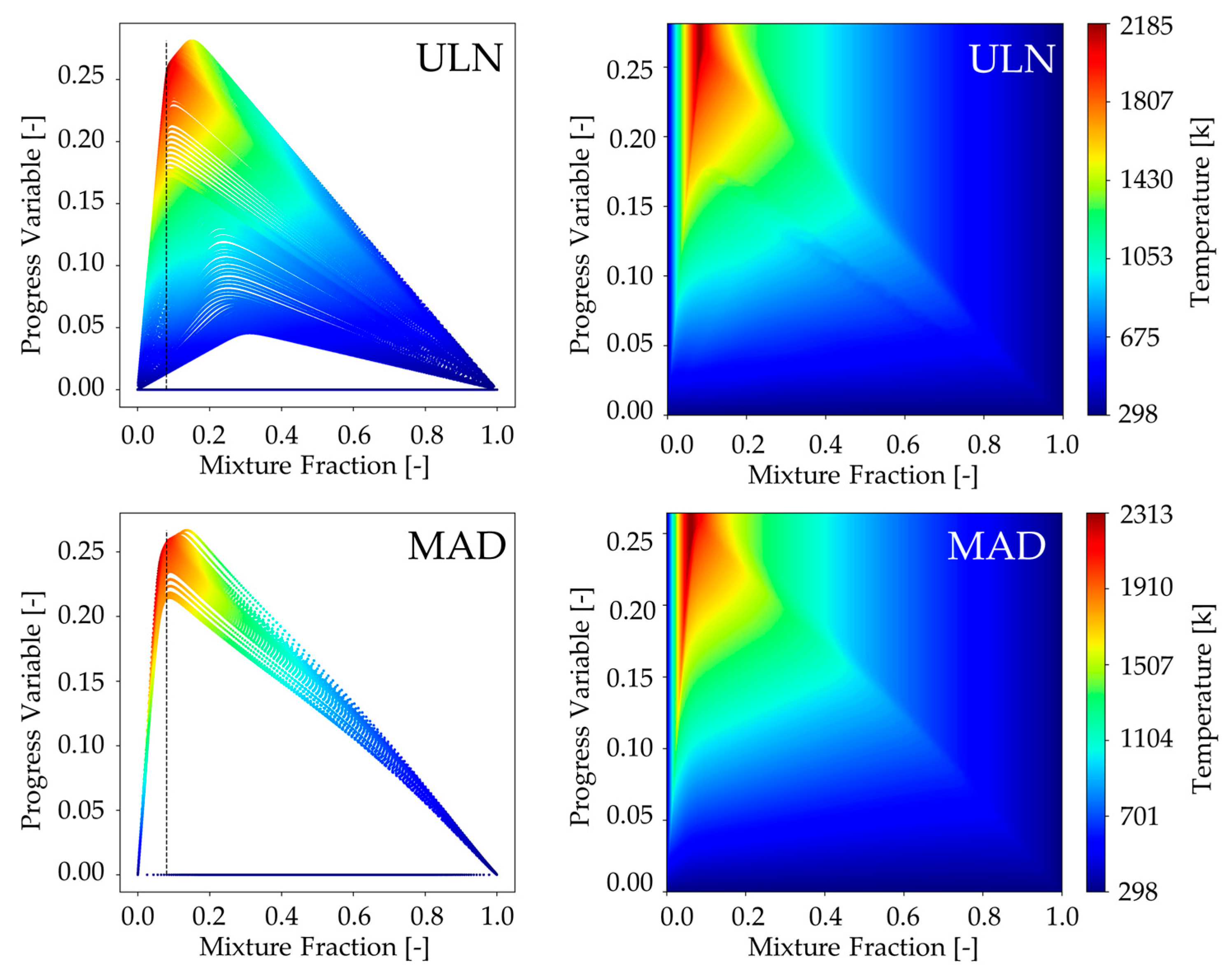
Figure 2 (left) presents the scatter plot of the progress variable against the mixture fraction, specifically for the adiabatic flame without variance in the mixture fraction, where each point is colored according to the temperature. The ULN Flamelet solution (top) shows a more concentrated distribution near the stoichiometric mixture fraction compared to the MAD model (bottom). This behavior is attributed to the ULN approach’s capability to capture the unstable branch of the S-curve, which improves solution continuity and resolution in the flame stabilization region. However, the obtained Flamelet library interpolates any missing data, resulting in both models appearing similar despite the differences in the original solutions, as demonstrated in Figure 2 (right). This interpolation introduces greater uncertainty in the MAD model, as a larger portion of its library is not directly solved but inferred. Such interpolation may be particularly critical when predicting the progress variable source term, which is extracted from the library during the LES, as illustrated in Figure 3 (right).

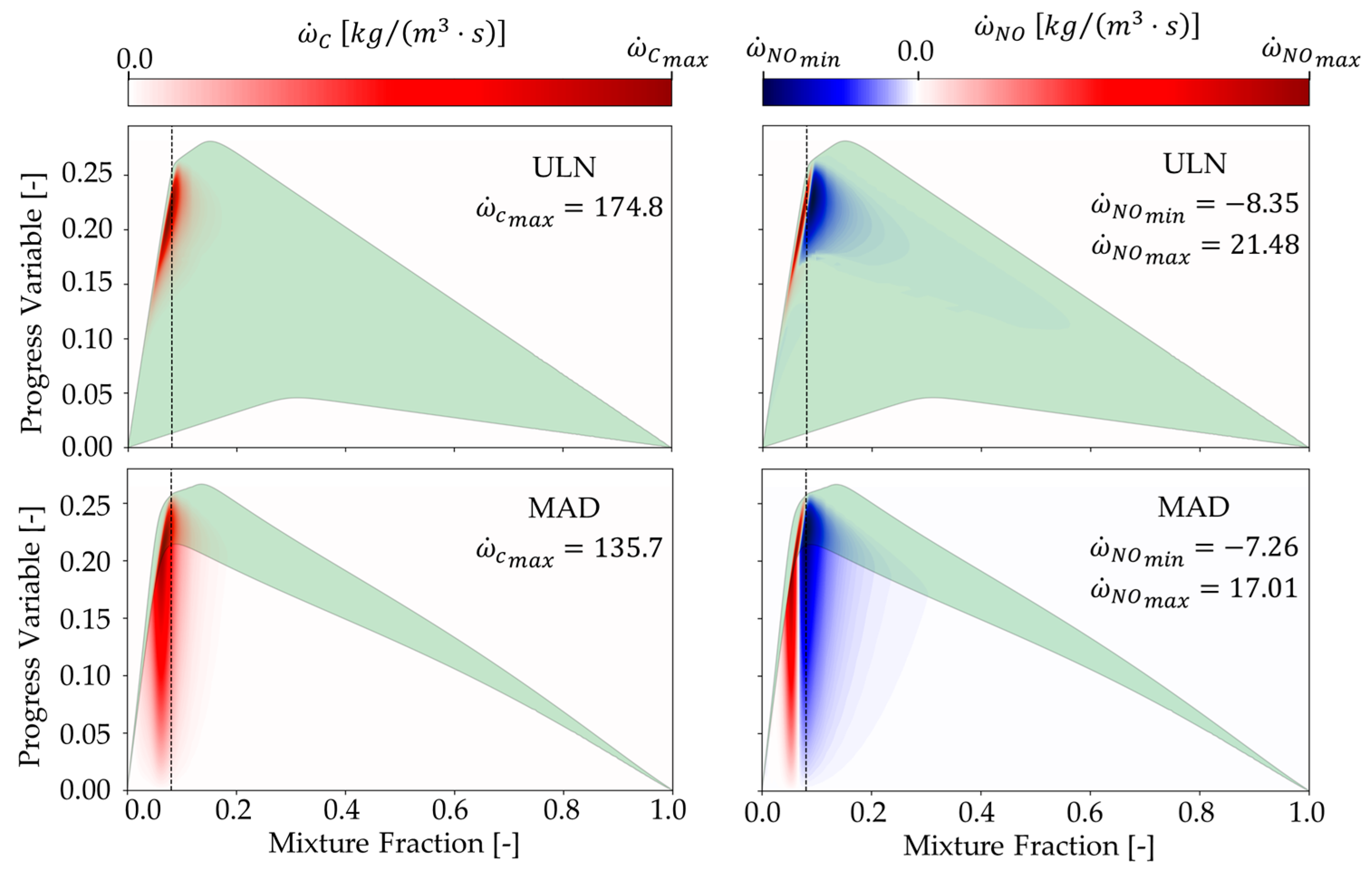
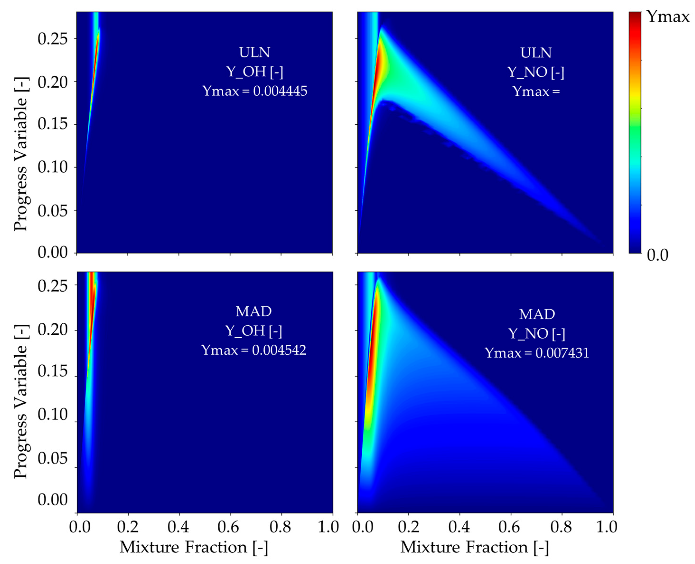
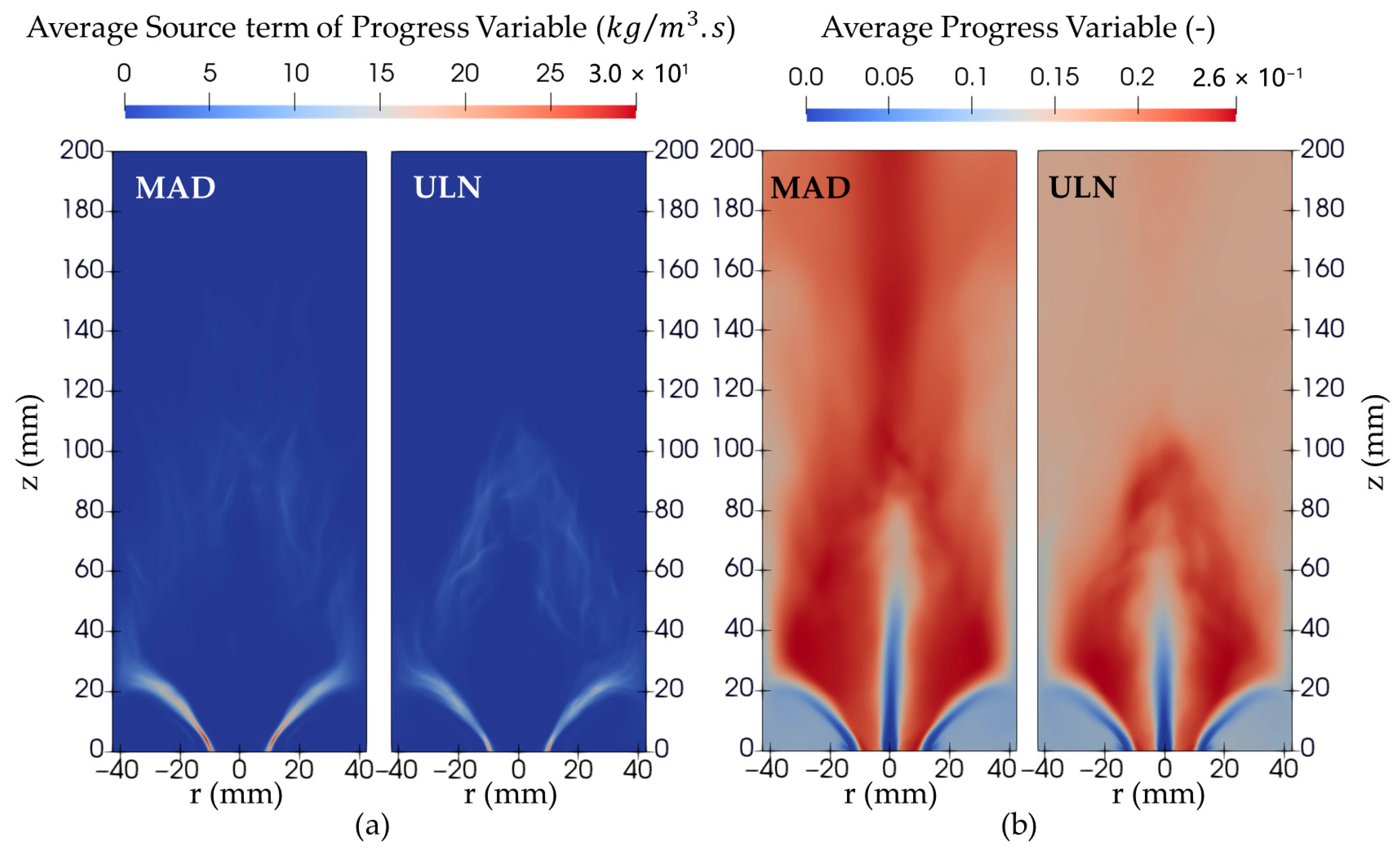
Figure 4 compares the distributions of $Y_{OH}$ and $Y_{NO}$ in the ULN and MAD Flamelet libraries, highlighting how DD affects their spatial behavior. Figure 3 further illustrates the source terms of the progress variable (left) and NO (right), using a seismic colormap in which red indicates production and blue indicates destruction. The green alpha shape marks the region where the Flamelet solution exists; outside this boundary, the Flamelet library is either interpolated or copied. This visualization highlights the dynamic balance between production and destruction in different flame regions and reveals the limitations of each model in covering the Flamelet library. It also provides insight into how diffusion models influence the key species responsible for pollutant formation and heat release.

In addition, the MAD library shows a narrower solved region compared to the ULN library. This gives an advantage to the ULN model, as during LES, the source terms for the progress variable and NO are retrieved from the library and substituted into the governing equations. A limited solved region in the MAD library may lead to inaccurate results due to the absence of unstable branch solutions.

In this study, special emphasis is placed on nitric oxide (NO) and hydroxyl radical (OH) due to their crucial roles in ammonia combustion chemistry. NO is a primary pollutant and one of the most harmful nitrogen-containing emissions, which is especially relevant in ammonia-based fuel systems where nitrogen content is inherently high. Its formation is governed by complex mechanisms, including prompt NO, thermal NO, and fuel NO pathways, all of which are influenced by flame temperature, local equivalence ratio, and radical pool composition.

OH, on the other hand, serves as a critical intermediate in the oxidation process and plays a key role in NO formation through reactions such as NH + OH → NO + H₂. It is also an indicator of high-temperature reaction zones and is often used to characterize flame front structures and heat release regions. Monitoring the OH distribution thus provides insight into the location and intensity of the reaction zones, while also indirectly informing about the potential for NO formation.

3. Results and Discussion

The presented results are time-averaged over 200,000 time steps, corresponding to an averaging period of approximately 30 ms. Since the experimental measurements include OH and NO distributions, the validation is carried out in Section 3.2.

3.1. Temperature Distribution and Flow Field

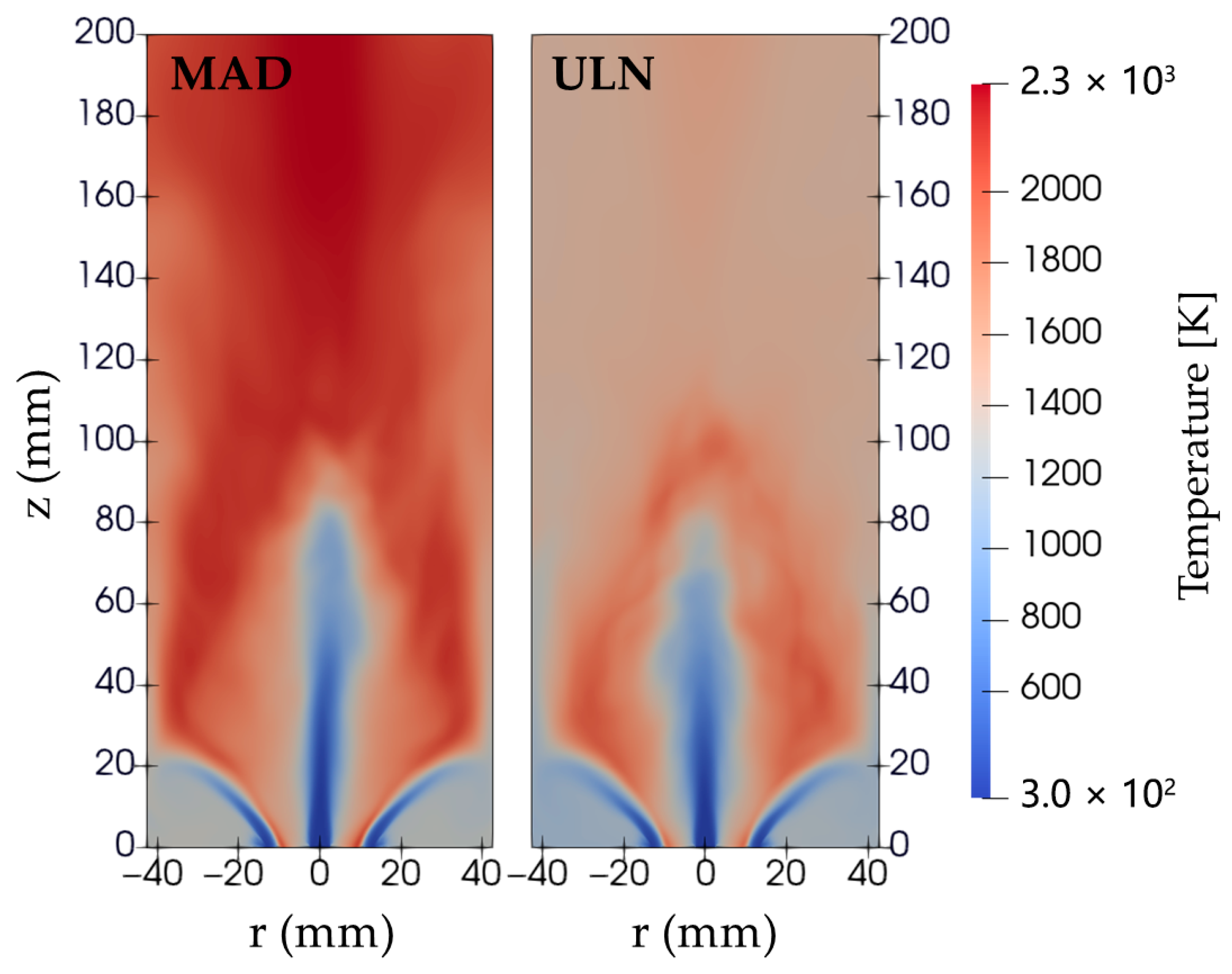
The temperature distribution in all MAD cases is noticeably higher than in the ULN cases, with unrealistically elevated temperatures observed downstream of the flame and away from the flame front, as shown in Figure 5. This raises concerns about the MAD model, which is expected to be more accurate due to its consideration of DD effects, unlike the ULN model, which suppresses these effects by assuming equal diffusivities for all species. However, the MAD model mispredicts scalar fields such as temperature and OH concentration, as will be further demonstrated in Section 3.2. This discrepancy is discussed in detail in that section.

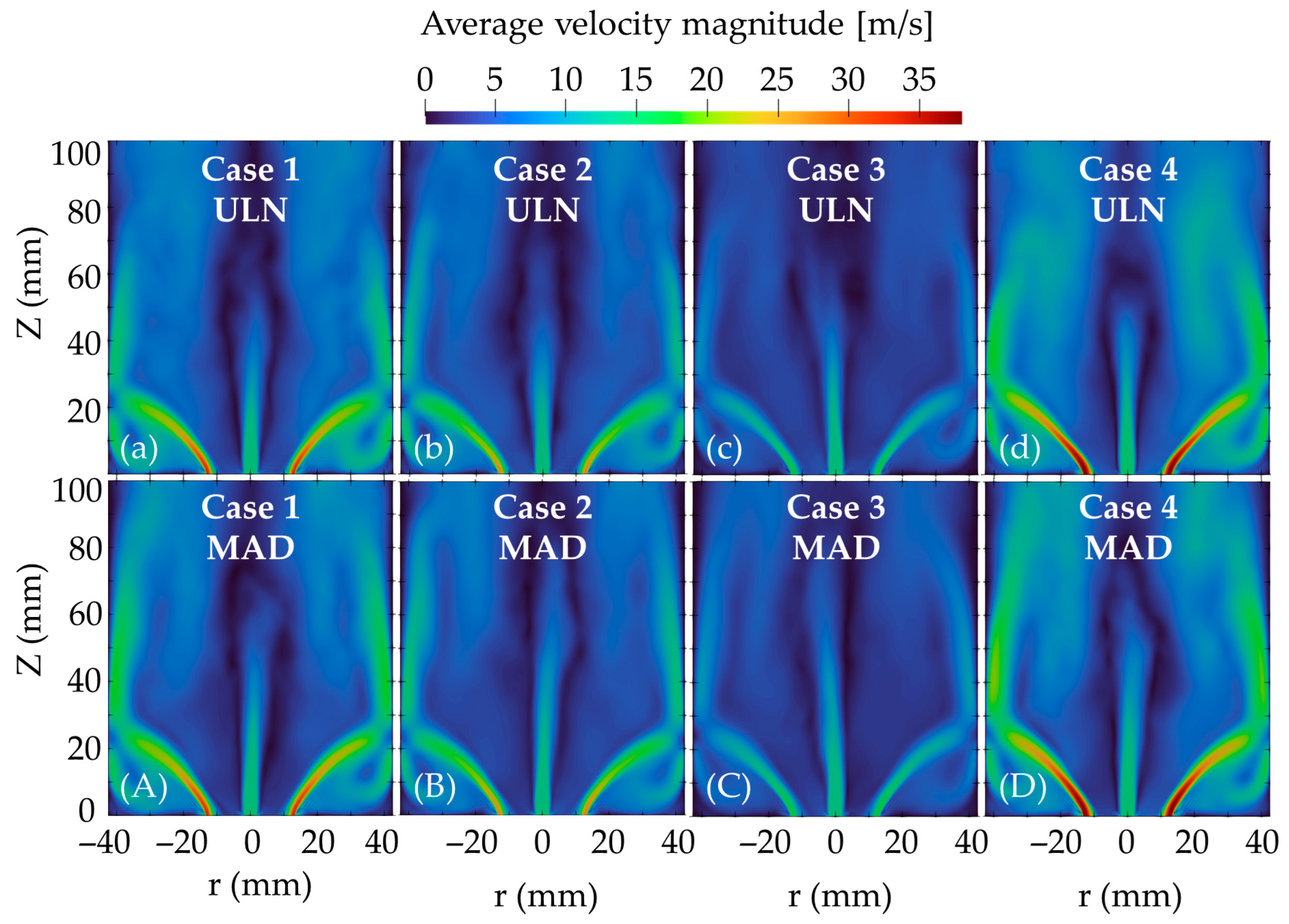
The flow field is primarily governed by the flow rates of the main streams and the geometry of the burner and combustor. Figure 6 shows the velocity magnitude distributions for the ULN model (top row, a–d) and the MAD model (bottom row, A–D). For the same swirl number (a–c and A–C), reducing the equivalence ratio increases the air flow rate, enhancing the swirling motion. However, increasing the swirl number has a more pronounced effect on swirl strength as in (b and d) or (B and D).

While the main flow structures are largely preserved, noticeable differences in velocity magnitude appear across the entire domain when comparing the two diffusion models. The MAD model shows higher velocity magnitudes over broader regions both inside and downstream of the flame, suggesting that enhanced diffusion contributes to stronger momentum transfer and a more sustained swirling motion.

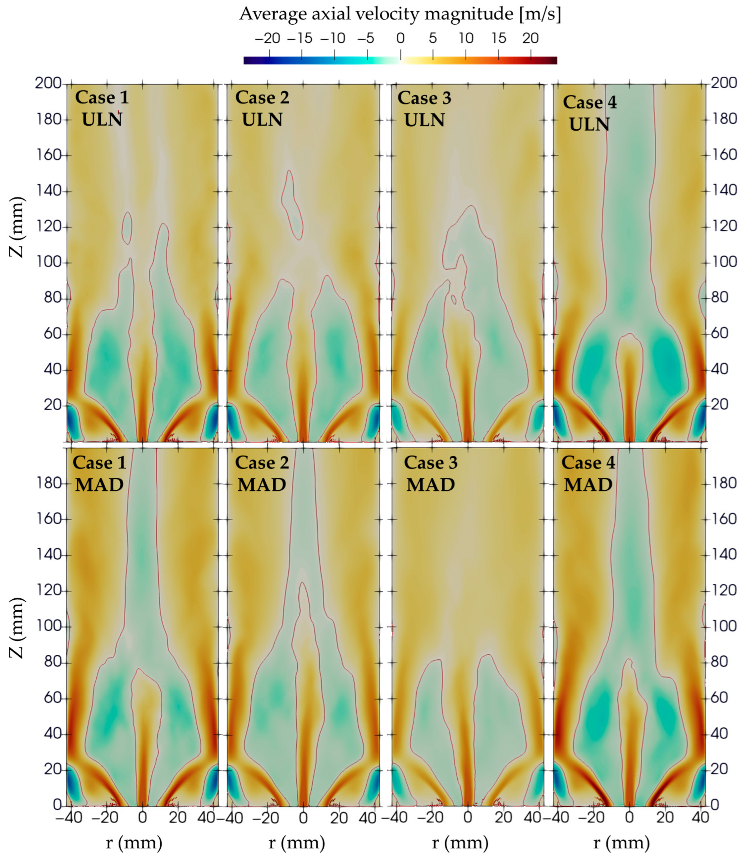
The velocity magnitude distribution shown in Figure 6 reveals that stronger swirling motion results in higher negative axial velocity in the central region of the combustor, as shown in Figure 7, both inside and downstream of the flame. This behavior is more pronounced in cases with higher swirl numbers, where the enhanced centrifugal force generates a stronger low-pressure zone along the axis. As a result, the central recirculation zone becomes more intense, drawing hot combustion products and reactants back toward the burner.

This recirculation not only contributes to flame stabilization but also enhances mixing between fuel and oxidizer, promoting more complete combustion. However, for low-reactivity fuels such as ammonia, CH₄/NH₃ blends do not always exhibit this behavior. As reported in [6], increasing the ammonia content reduces the influence of swirl on flame stability. Beyond a certain blend ratio, higher swirl numbers may even worsen flame stability. This is attributed to the strong shear regions created by intense recirculation, where the variance of the mixture fraction is also intense, which negatively affects the slow chemical kinetics of ammonia oxidation.

Moreover, the MAD model consistently exhibits stronger negative axial velocities compared to the ULN model, suggesting that the diffusion formulation in MAD enhances the momentum transfer and supports a more vigorous swirling motion. These differences indicate that both the swirl number and diffusion model play a significant role in shaping the flow field and, consequently, combustion characteristics.

3.2. Effect of Diffusion Model on NO/OH Distribution and Kinetics

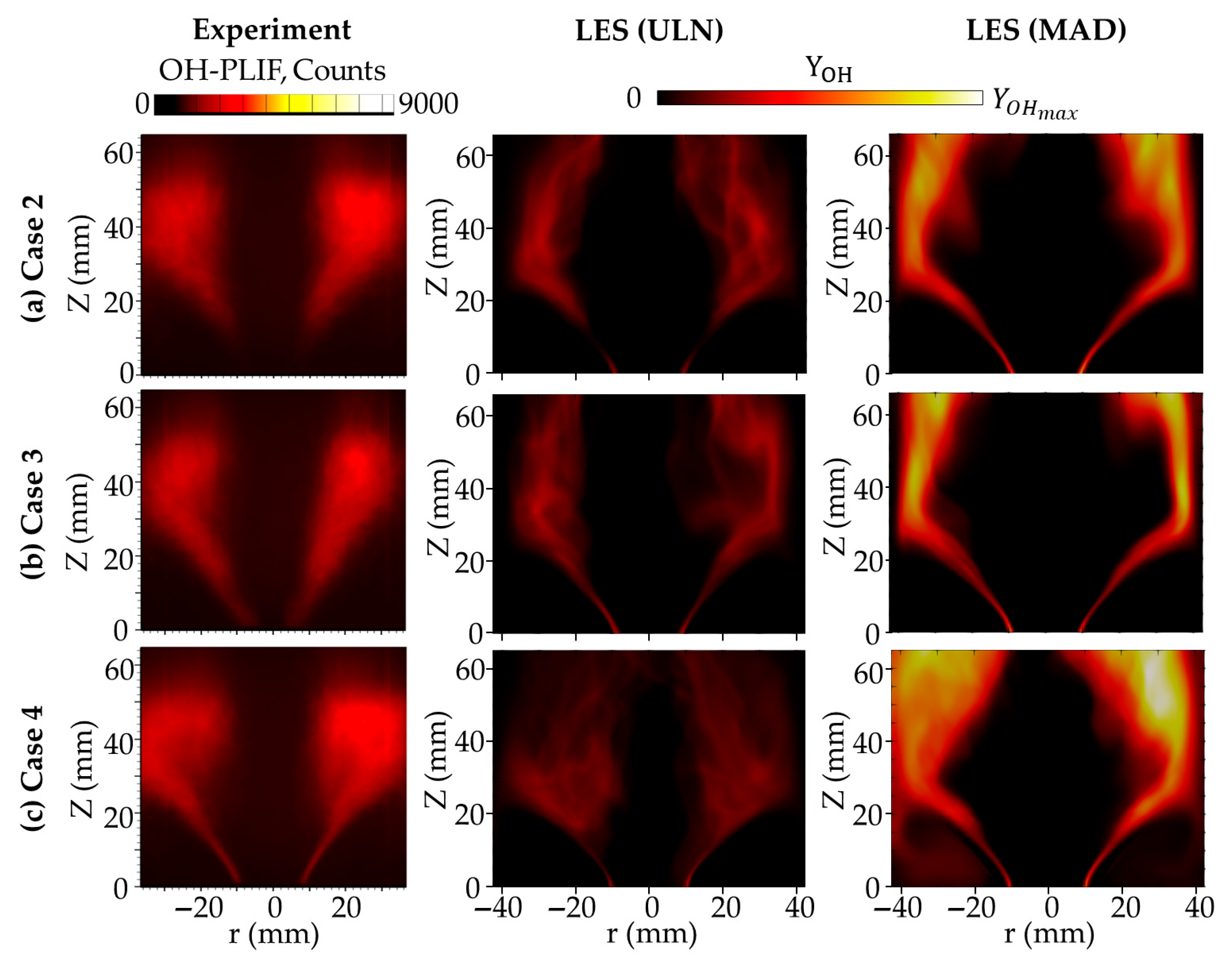
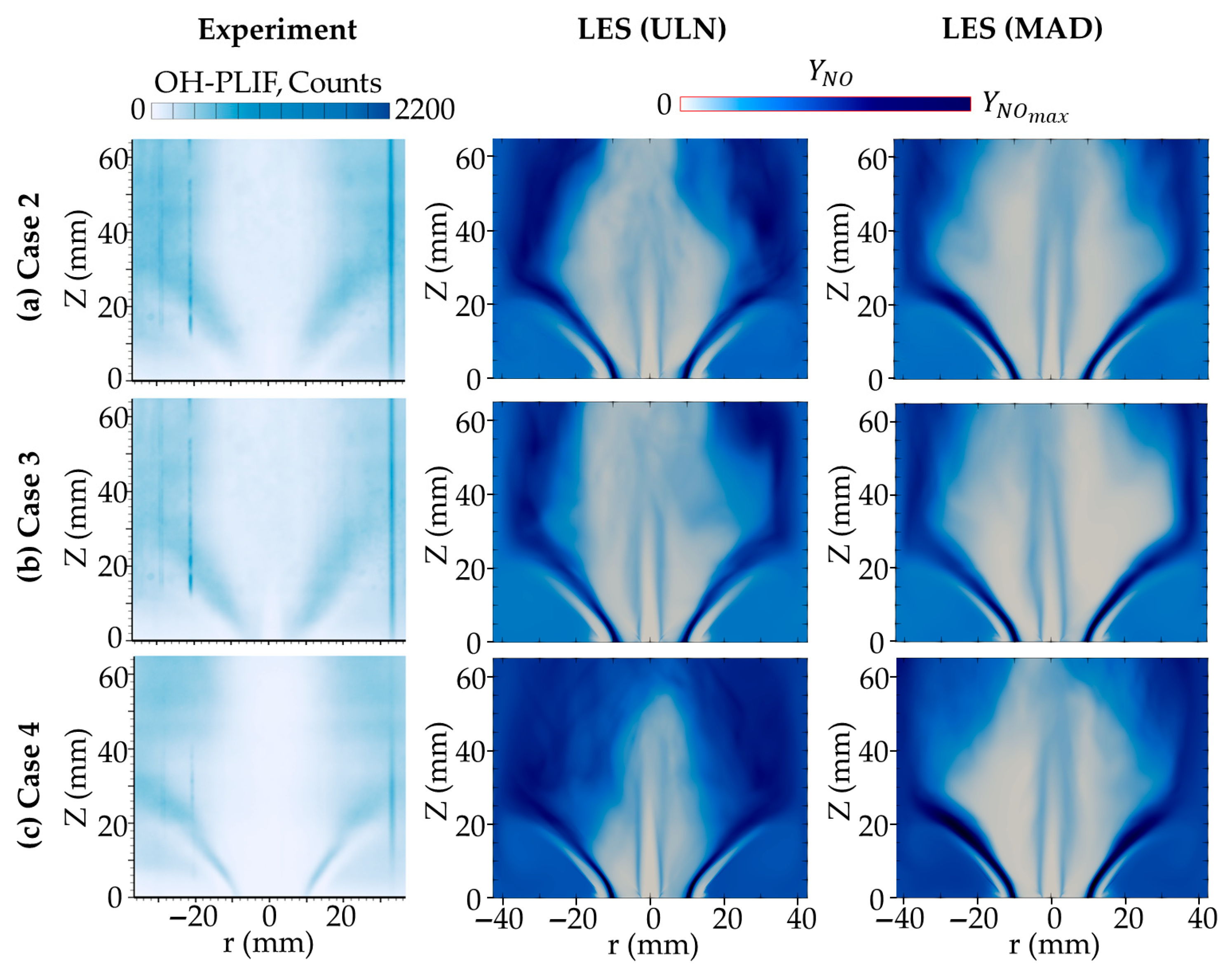
Figure 8 compares the time-averaged OH mass fraction distributions predicted by the ULN and MAD models with experimental PLIF data [6], while the NO mass fraction is shown in Figure 9. The OH distribution predicted by the ULN model shows better agreement with the experimental measurements, while the MAD model exhibits a noticeably narrower OH region near the burner, indicating the stronger confinement of radical species due to DD. For NO, both models capture the general distribution reasonably well, although differences exist: the MAD model predicts a slightly narrower NO region compared to ULN, yet both remain in an acceptable agreement with the experimental profile. Downstream of 65 mm from the burner rim, the MAD model shows a more extended tail in NO concentration as shown in Figure 10a; however, due to the lack of experimental data in this region, the accuracy of this prediction cannot be confirmed. In addition, the OH distribution in this region is high as well for MAD cases.

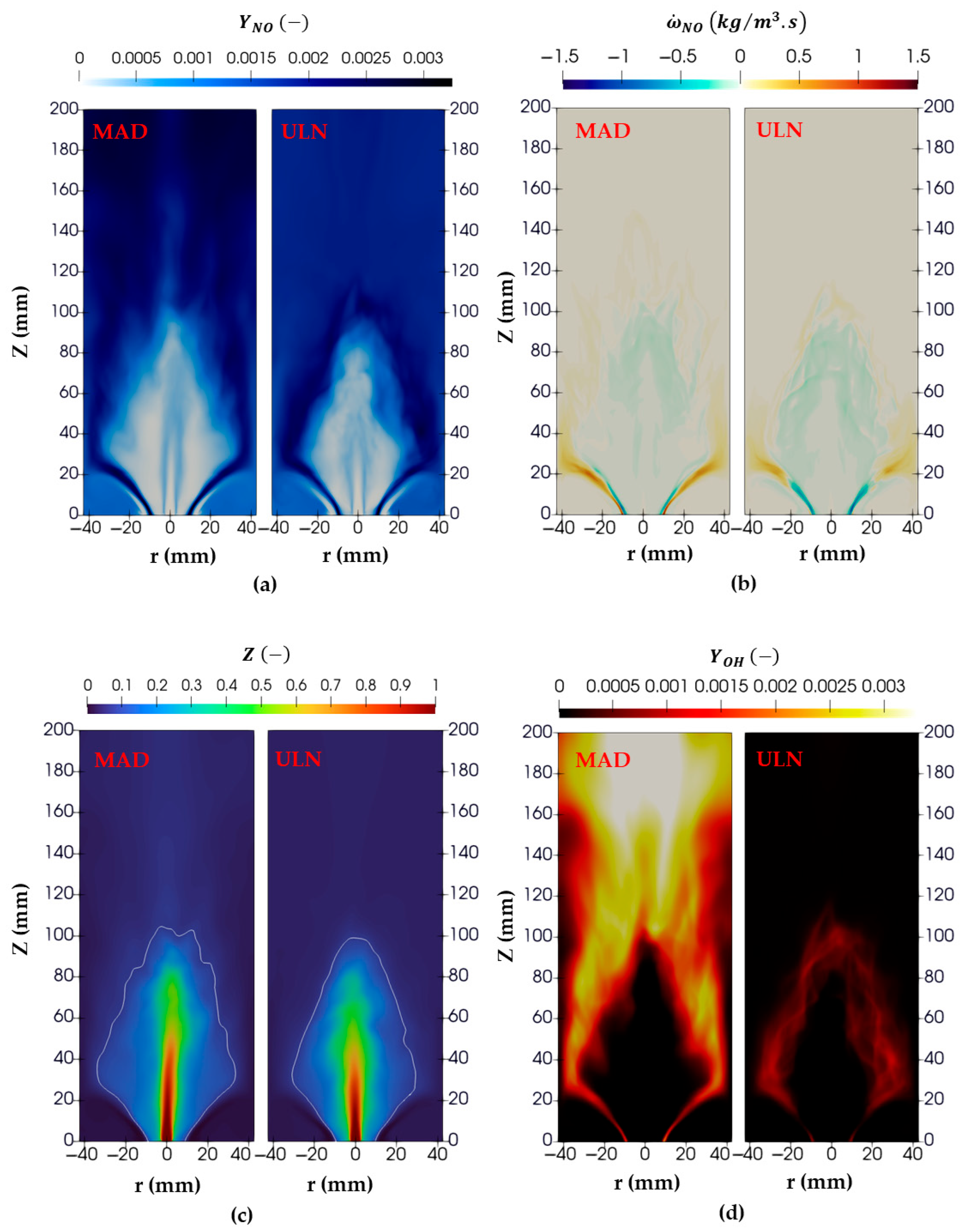
Although the diffusion model only has a minor impact on the overall flow field, it significantly affects the NO distribution and its source term. Figure 10a shows the NO mass fraction distribution for Case 2 using both the ULN and MAD models. In the MAD case, higher NO concentrations are observed further downstream of the flame, while in the ULN case, the peak NO concentrations are localized near the flame front.

The differences in NO distribution around the flame front between the ULN and MAD models arise primarily from how species diffusion is treated. In the ULN model, the assumption of equal diffusivity for all species leads to a more localized flame front, where peak temperatures and reaction rates align, resulting in an NO formation concentrated near the front. In contrast, the MAD model accounts for species-specific diffusivities, allowing the faster diffusion of reactive radicals such as OH and O. This broadens the flame structure and promotes NO formation farther downstream. However, the high NO concentrations observed downstream, despite mixing with excess air, are not realistic and are attributed to the artificial increase in the progress variable, as will also be discussed later in this section for OH.

This is evident in the NO source term distribution shown in Figure 10b. In the ULN case, the source term is predominantly negative in the early flame stages near the burner rim, indicating NO consumption. In contrast, the MAD case shows both positive and negative source terms in the same region, reflecting ongoing NO production. This behavior is attributed to the interpolated NO source term shown in Figure 3 (left and bottom), which appears artificially high due to interpolation. This occurs because NO is not directly solved in the Flamelet model within the unstable branch region, which lies between the lowest stable branch and the quenching branch.

The NO source term is retrieved from the Flamelet library during the LES calculations. As a result, the artificially high source term leads to excessive NO production, which is then transported downstream with unrealistically high values.

The OH mass fraction distribution shown in Figure 10d for case 2 indicates that the MAD model predicts elevated OH concentrations downstream of the flame front, in the flue gas region where it mixes with excess air. This behavior is consistent across all other cases as well. Consequently, the progress variable also exhibits higher values in these regions for MAD cases, as illustrated in Figure 11b. This trend can be traced back to the distribution of the progress variable source term, which is concentrated near the burner rim in the early stages of the flame. Since the LES framework solves the transport equation for the progress variable by sampling its source term from the precomputed Flamelet library, any interpolation artifacts in the library are directly reflected in the LES results.

In the case of the MAD model, a substantial portion of the Flamelet library—particularly between the extinction curve (where the progress variable equals zero) and the lowest stable computed Flamelet—is not explicitly solved but interpolated. This is shown in Figure 2 (left) and Figure 3 (left) for the MAD library. This unsolved region is significantly larger in MAD than in the ULN model, primarily due to the absence of unstable branch solutions in MAD. Furthermore, source term values above the highest stable curve are often extrapolated or copied from the highest computed solution, which adds to the inaccuracy.

These limitations in the MAD library contribute to an overprediction of the progress variable and OH mass fraction, both downstream of the flame and within the flame itself. The broader region of positive source term values in the MAD library—caused by interpolation across the high-progress-variable zone where unstable branches typically exist—leads to a more rapid increase in the progress variable throughout the combustion domain.

3.3. Effect of Swirl Number on NO Emissions

As discussed earlier in Figure 6, increasing the swirl number alters the shape of the flow field as expected. Figure 12 further illustrates the impact of swirl numbers 8 and 12 on the NO mass fraction and source term distributions in the ULN model. A higher swirl number shortens the reaction region while intensifying the NO source terms near the burner rim. As a result, NO production becomes more concentrated in the early stages of the flame, whereas NO consumption is more broadly distributed downstream with lower intensity. As observed in [6], increasing the swirl number leads to similar NO emissions across different NH₃/CH₄ blends. This trend is attributed to the enhanced central recirculation and flame stabilization at high swirl, which promotes intense combustion and NO production near the burner. Under these conditions, the flame is shorter, and most NO is produced in the early stages via the thermal and fuel-bound nitrogen pathways, with limited residence time for downstream reduction. In contrast, lower swirl numbers produce a more extended flame with longer residence times and distributed heat release, allowing blend-specific differences in NO production and post-flame reduction pathways to become more pronounced. Consequently, the NO emissions become more dependent on the NH₃/CH₄ blend ratio under lower swirl conditions.

3.4. Effect of Global Equivalence Ratio on Flame Structure and NO Emissions

In this study, the fuel is supplied at a fixed velocity of 13 m/s for all cases. Therefore, changes in the global equivalence ratio are achieved solely by adjusting the air mass flow rate, which is inherently higher than that of the fuel. As a result, this method can also introduce momentum effects into the flow field. The flame shape changes accordingly, as a lower global equivalence ratio has a similar effect to increasing the swirl number but not the same. It enhances the velocity magnitudes and strengthens the swirling motion, as shown in Figure 6; on the other hand, the swirl number controls tangential and axial momentum ratios. Consequently, varying the global equivalence ratio significantly influences the flame structure and its emissions, including NO.

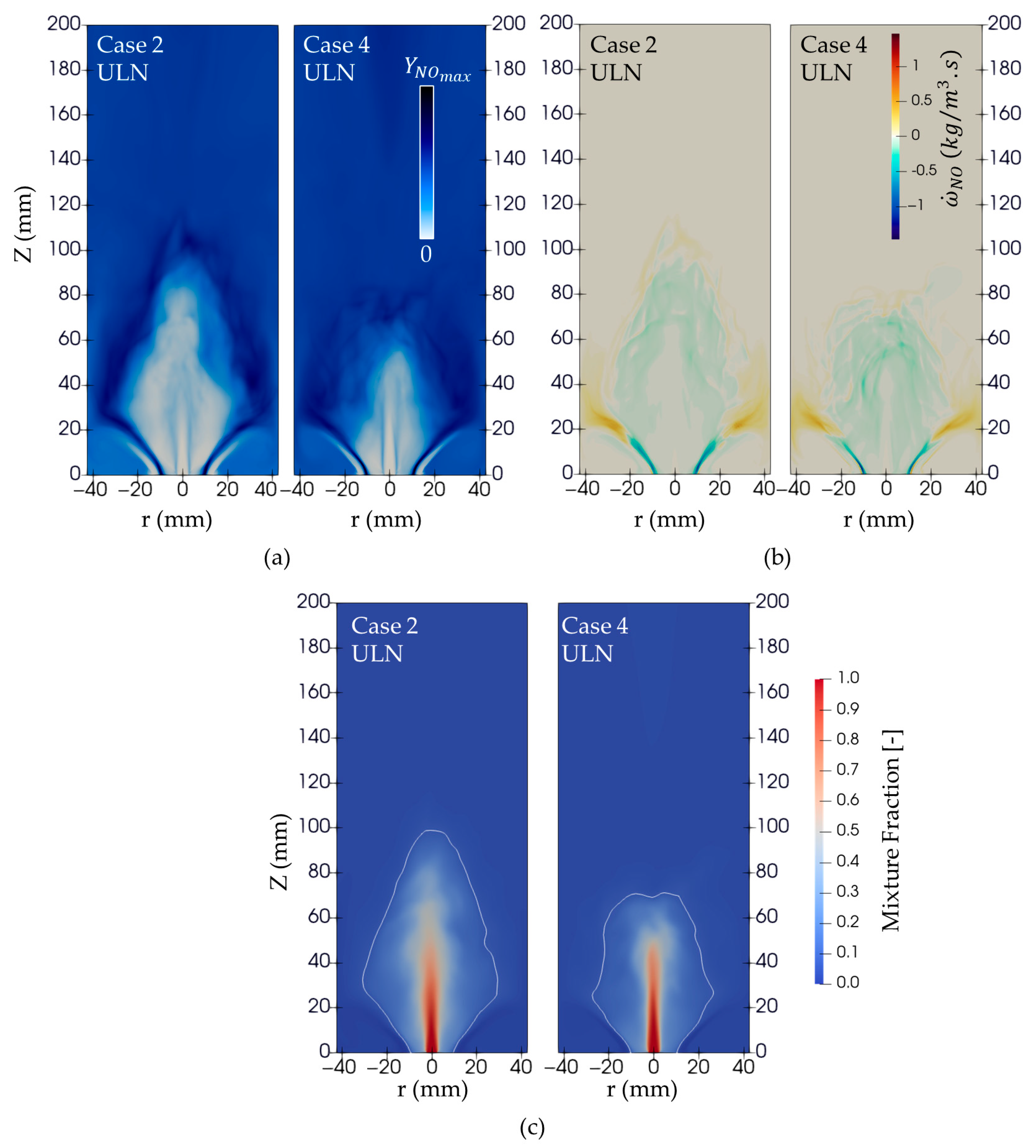
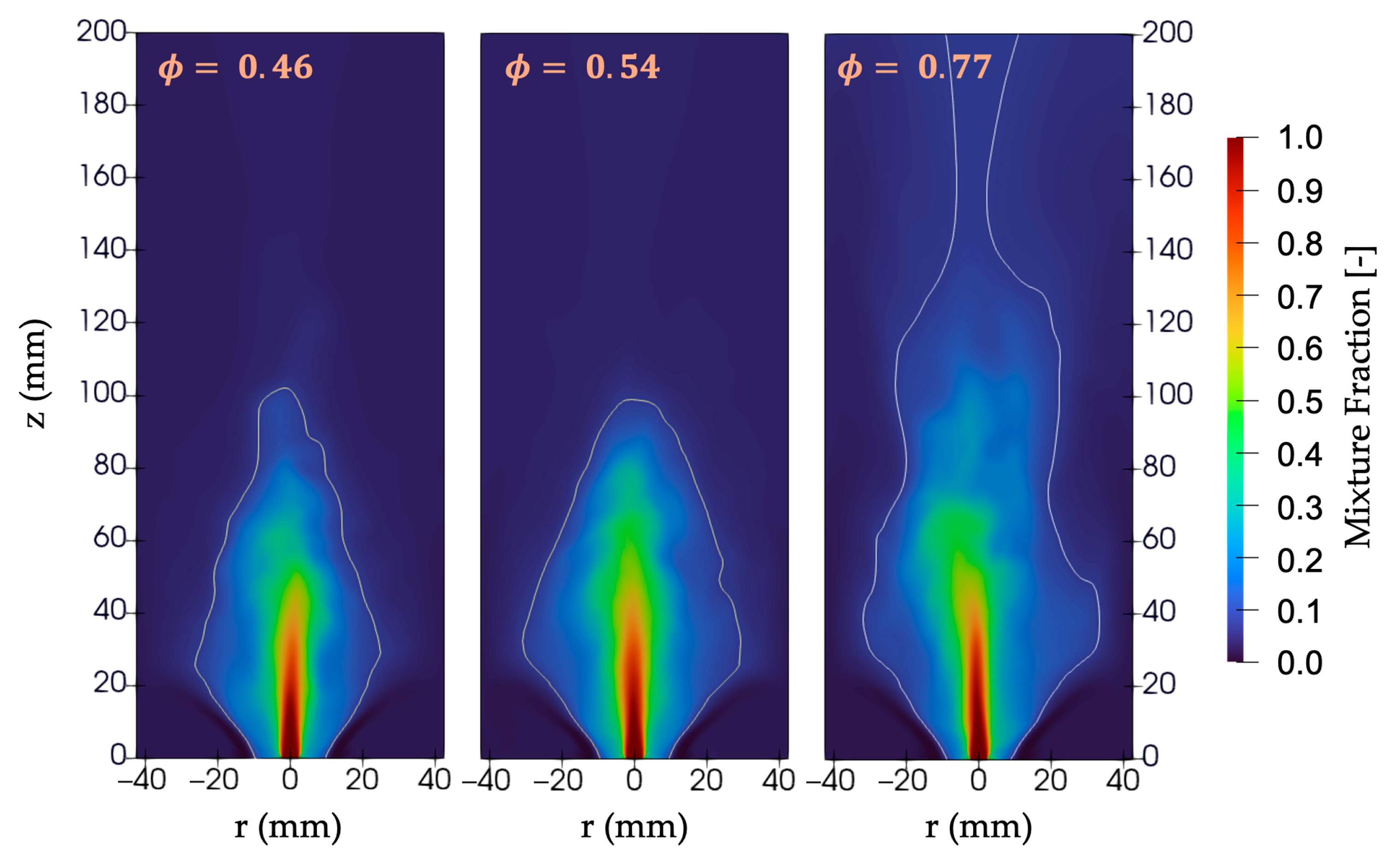
Figure 13 shows the mixture fraction fields for cases 1, 2, and 3 using the ULN model. At a high equivalence ratio (0.77), the air momentum is relatively low compared to the fuel jet, preventing proper interaction between the swirling air and the fuel jet. This results in poor combustion. In contrast, lower global equivalence ratios (0.54 and 0.46) introduce a greater amount of air and higher air momentum, enhancing the air–fuel mixing. This leads to a reduction in the mixture fraction below the stoichiometric value throughout the domain, around 100 mm downstream of the burner rim, indicating improved combustion. Furthermore, although the mixing process improves at lower equivalence ratios, the flame length remains nearly identical for both cases. This is because, in non-premixed combustion, once sufficient mixing is achieved, the diffusion process becomes the dominant factor governing combustion, leading to similar flame lengths. However, as mentioned in Section 3.3, increasing the swirl number has the strongest effect on the flow field, resulting in shorter flames, and therefore increasing the swirl number can improve the combustion process for a high equivalence ratio like 0.77, as mentioned in [6].

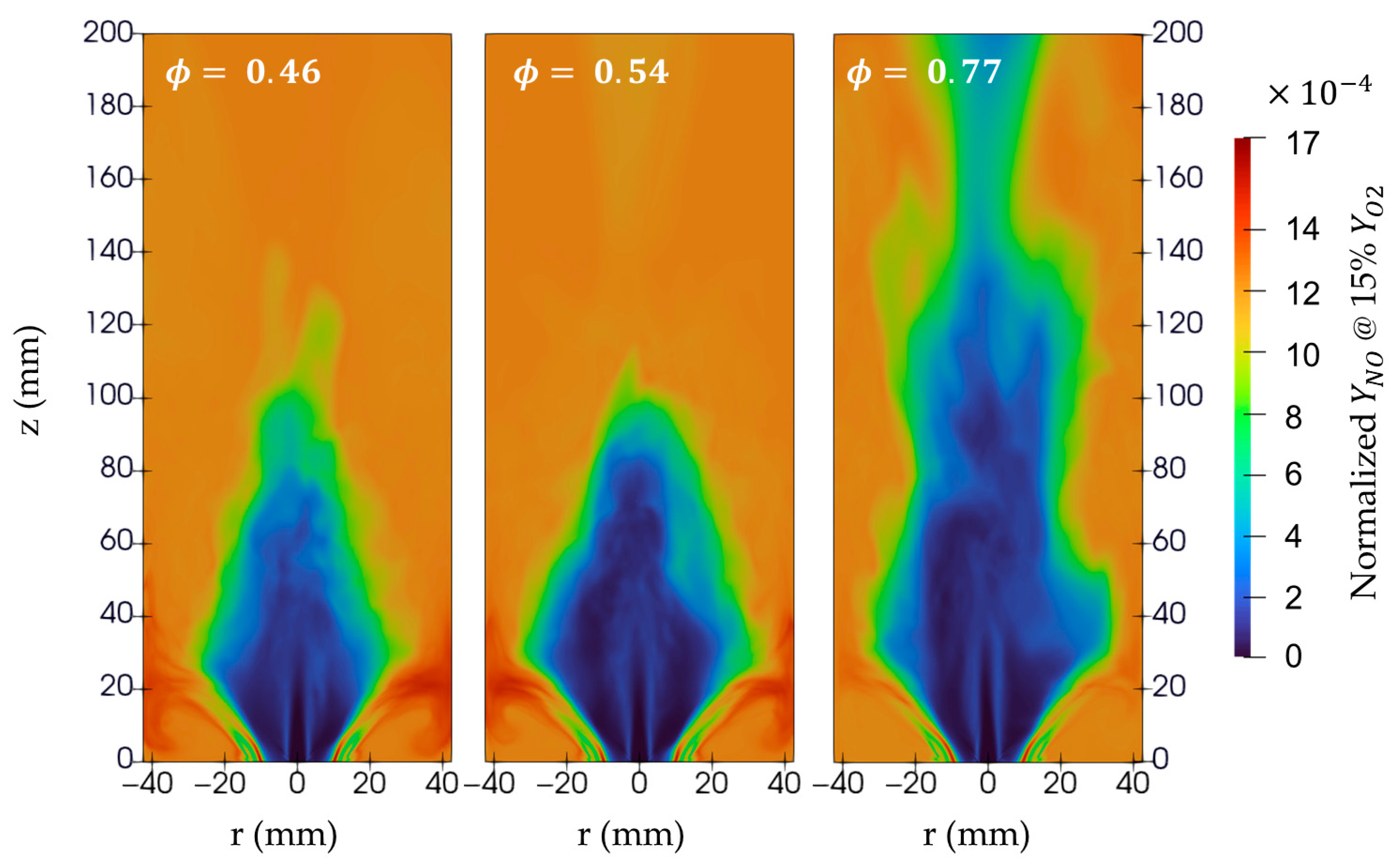
Figure 14 shows the normalized NO mass fractions at 15% O₂ mass fractions, this normalization process serves to eliminate the effect of different amounts of air associated with different equivalence ratios on the NO mass fraction. The high global equivalence ratio shows the lowest maximum NO mass fractions among the maxima of the three cases, which is expected due to the poor combustion process, which exhibits lower NO and higher NH₃ emissions, as mentioned in [6]

4. Conclusions

This study investigated the effects of the swirl number and diffusion modeling on the flow field and NO emissions in CH₄/NH₃ flames. Large eddy simulations (LES) were conducted for a 50% ammonia/50% methane mixture by volume, across various equivalence ratios and swirl numbers. Two diffusion models were considered: the unity Lewis number (ULN) model and the mixture-averaged diffusion (MAD) model. Several cases were selected to match those in [6] for comparison.

The key findings are as follows:

• While the choice of diffusion model has a minor effect on the overall flow field, it significantly influences flame structure, and the distribution of reactive species.
• The MAD model predicts higher OH concentrations and broader reaction zones compared to the ULN model, which better matches experimental OH profiles with more localized flame structures. This overprediction in the MAD case arises from artificially elevated progress variable source terms in the Flamelet library, particularly in regions where an unstable branch was not resolved, unlike the ULN model, which successfully recovers this branch. As a result, the MAD model exhibits exaggerated progress variable growth throughout the flame.
• For NO emissions, the ULN model confines NO formation and reduction to a narrow region near the flame front, whereas the MAD model shows more spatially distributed NO profiles, driven by differential diffusion (DD) of nitrogen-based intermediates.
• Increasing the swirl number leads to shorter flames and upstream-shifted NO formation zones. This limits the role of post-flame NO chemistry and suppresses NO reduction pathways associated with intermediate species such as NH and NH₂.
• Reducing the global equivalence ratio to a certain level ensures good air–fuel mixing near the burner rim, leading to improved combustion. This is associated with reduced fuel slip to the exhaust and increased NO emissions.
• Future work includes the development of unstable branch calculation for the MAD model to enable accurate resolution for it and reduce interpolation artifacts in the Flamelet library. These findings enhance the understanding of how diffusion models and turbulent flow conditions influence NO chemistry in ammonia–methane flames and can inform strategies for low-emission combustion design.