A Mid-Term Scheduling Method for Cascade Hydropower Stations to Safeguard Against Continuous Extreme New Energy Fluctuations

Abstract

Continuous multi-day extremely low or high new energy outputs have posed significant challenges in relation to power supply and new energy accommodations. Conventional reservoir hydropower, with the advantage of controllability and the storage ability of reservoirs, can represent a reliable and low-carbon flexibility resource to safeguard against continuous extreme new energy fluctuations. This paper proposes a mid-term scheduling method for reservoir hydropower to enhance our ability to regulate continuous extreme new energy fluctuations. First, a data-driven scenario generation method is proposed to characterize the continuous extreme new energy output by combining kernel density estimation, Monte Carlo sampling, and the synchronized backward reduction method. Second, a two-stage stochastic hydropower–new energy complementary optimization scheduling model is constructed with the reservoir water level as the decision variable, ensuring that reservoirs have a sufficient water buffering capacity to free up transmission channels for continuous extremely high new energy outputs and sufficient water energy storage to compensate for continuous extremely low new energy outputs. Third, the mathematical model is transformed into a tractable mixed-integer linear programming (MILP) problem by using piecewise linear and triangular interpolation techniques on the solution, reducing the solution complexity. Finally, a case study of a hydropower–PV station in a river basin is conducted to demonstrate that the proposed model can effectively enhance hydropower’s regulation ability, to mitigate continuous extreme PV outputs, thereby improving power supply reliability in this hybrid renewable energy system.

1. Introduction

With the rapid advancement of the economy, energy demand has been continuously increasing [1,2]. The widespread use of fossil fuels to meet this growing demand has become one of the primary drivers of global climate change, highlighting the urgent need to develop clean and renewable energy sources [3,4,5,6]. In recent years, as renewable energy technologies—particularly wind and solar power—have advanced, their integration into modern power systems has increased significantly. Consequently, the inherent variability and intermittency of these resources have posed growing challenges regarding power system stability. This issue is exacerbated by climate change, leading to more frequent and severe extreme weather events like heatwaves, cold spells, and typhoons [7]. These events are often sudden, wide-ranging, and prolonged, resulting in continuous and extreme fluctuations in renewable energy outputs over multiple days. Such extreme volatility presents substantial challenges in maintaining the power and energy balance of the grid [8,9,10,11].

To mitigate extreme fluctuations in renewable energy outputs, energy storage technologies have been widely developed [12]. Storage systems absorb excess power during high VRE outputs and release it during low-output periods [13]. By the end of 2024, the global storage capacity reached 372 GW, with pumped hydro and lithium-ion batteries accounting for 52.8% and 42.1%, respectively. Pumped hydro mainly provides intra-day peak shaving [14,15,16], while lithium-ion batteries focus on peak and frequency regulation [17]. Long-duration storage still faces challenges in terms of cost and reliability [18]. In contrast, hydropower reservoirs provide flexible, controllable dispatch with storage and ramping capabilities [19,20,21,22], making them vital in integrating VRE and ensuring system stability.

The core principle of wind–solar–hydropower coordination is to exploit hydropower’s flexibility to mitigate wind and solar variability and uncertainty [23,24]. This multi-energy integration enhances renewable accommodation and strengthens the overall system stability. Two challenges are critical: first, accurately characterizing renewable uncertainty across multiple timescales, including the robust modeling and forecasting of rapid and continuous fluctuations [25], and second, devising an efficient co-scheduling framework for hydropower, wind power, and solar power that fully harnesses hydropower’s flexibility through coordinated optimization at the system level [26,27,28]. Overcoming these issues is essential in advancing power systems toward a high level of renewable energy integration.

To address the characterization of renewable energy uncertainty, extensive research has been conducted. This uncertainty mainly stems from the intermittency and variability of renewable resources [8], driven by meteorological factors such as temperature, solar radiation, and wind speed [29]. The output of renewables shows significant temporal and spatial correlation, complicating forecasting and operational planning. To address this, stochastic optimization methods based on discrete probability distributions [30,31,32], particularly scenario analysis, have been widely used to enhance the dispatch robustness and system reliability.

Mainstream scenario generation methods for renewable energy uncertainty fall into two categories [33]: sampling-based and prediction-based approaches [34,35]. Sampling-based methods rely on historical data to derive probability distributions, using techniques such as Monte Carlo (MC) [36], Latin Hypercube Sampling (LHS) [37], and Gibbs sampling [38], to preserve statistical characteristics and reflect inherent randomness. In contrast, prediction-based methods employ data-driven models to simulate future renewable outputs under varying conditions. These include autoregressive moving average (ARMA) models [39] for capturing temporal dependencies and machine learning algorithms, such as artificial neural networks (ANNs) and support vector machines (SVMs) [40], which learn complex nonlinear relationships between meteorological inputs and generation patterns. With the rise of artificial intelligence and big data analytics, prediction-based approaches are gaining attention for their improved accuracy in scenario generation.

Numerous methods have been developed for the complementary dispatch of hydropower and variable renewable energy under uncertainty. For a long-term horizon, such dispatch leverages the annual regulation capacity of key hydropower stations and the seasonal complementarity of renewables to ensure stable integration under variable inflows. Ref. [41] transforms a multi-stage optimization into a two-stage model to improve the computational accuracy. Ref. [42] formulates a multi-objective model that maximizes generation and reliability within a long-term complementary framework. Ref. [43] applies a stochastic optimization incorporating simulated electricity prices, solved via discrete differential dynamic programming with operating rules derived from implicit stochastic optimization, to support market-based hydro–wind–solar coordination. Additionally, Ref. [44] develops a mid-to-long-term input–output dispatch model for cascade hydropower–PV systems, addressing operational complexities and uncertainties to effectively reduce the impact of forecasting errors. For a short-term horizon, dispatch must leverage hydropower flexibility within system constraints to manage stochastic renewable fluctuations and reverse peak shaving [45]. Ref. [46] introduces an extended planning model with operational flexibility constraints to reconcile variability across long- and short-term horizons and enhance renewable integration. Ref. [47] develops a short-term economic dispatch model for a hydropower–PV–pumped storage system, solved via an MOEA/D algorithm to jointly optimize the output stability and economic benefits under ancillary service participation. Ref. [48] proposes a short-term MILP scheduling model for cascade energy storage–wind–solar systems, integrating unit-level constraints, hydraulic coupling, and grid limitations and employing piecewise linearization with three-dimensional interpolation for nonlinear components.

Unlike the stable long-term seasonal fluctuations and high accuracy of short-term output forecasting, renewable energy exhibits significant uncertainty on a mid-term timescale. This study addresses the critical gap in hydro–wind–solar complementary scheduling at weekly–monthly timescales, where existing research predominantly focuses on either short-term (day-ahead/intra-day) or annual/monthly resolutions. To mitigate persistent multi-day renewable fluctuations, we propose a two-stage stochastic optimization framework for cascade hydropower. The methodology involves (1) generating extreme PV scenarios via Monte Carlo sampling with Synchronized Backward Reduction; (2) formulating and solving a stochastic optimization model accommodating PV uncertainty; (3) validating the approach through comparative simulations against deterministic models using basin hydropower case data. The results demonstrate enhanced compensation capability for sustained renewable volatility and improved operational stability in hydro–solar systems.

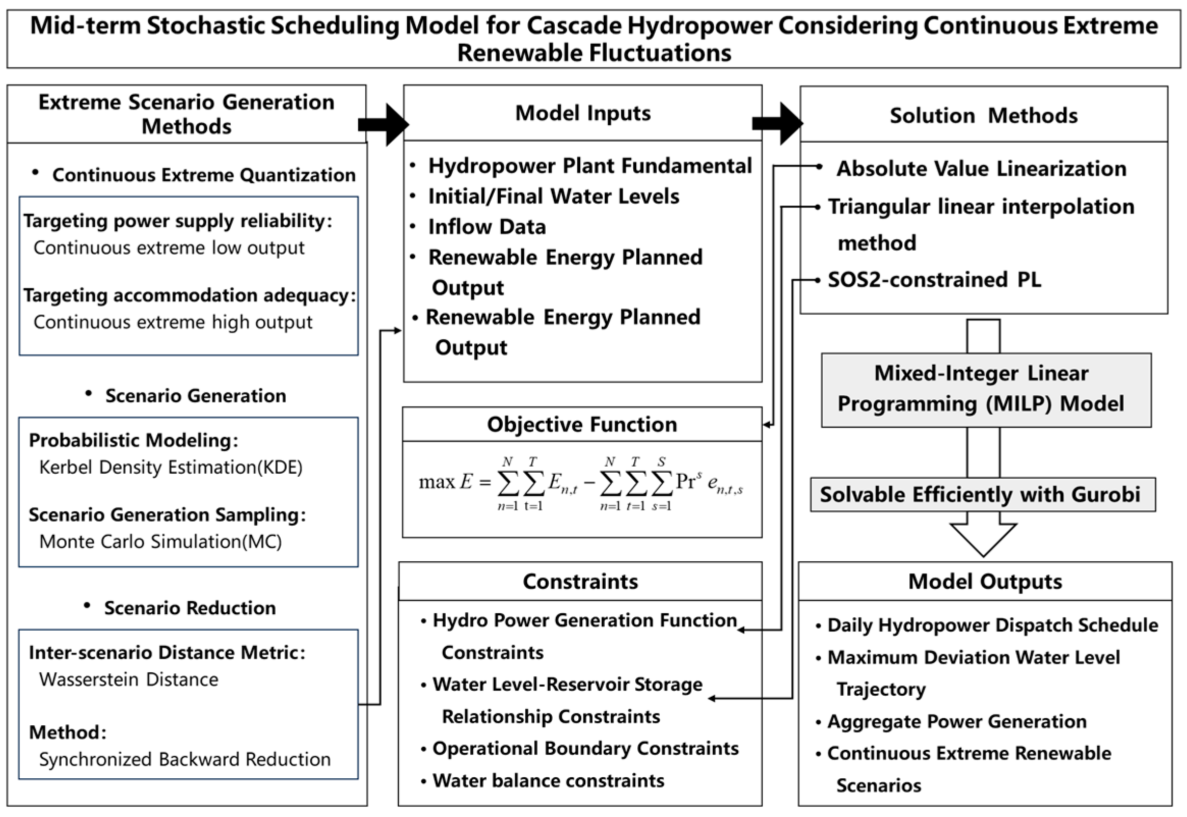
2. Methodology

The methodological framework employed in this study is illustrated in Figure 1.

2.1. Extreme Scenario Generation Methods

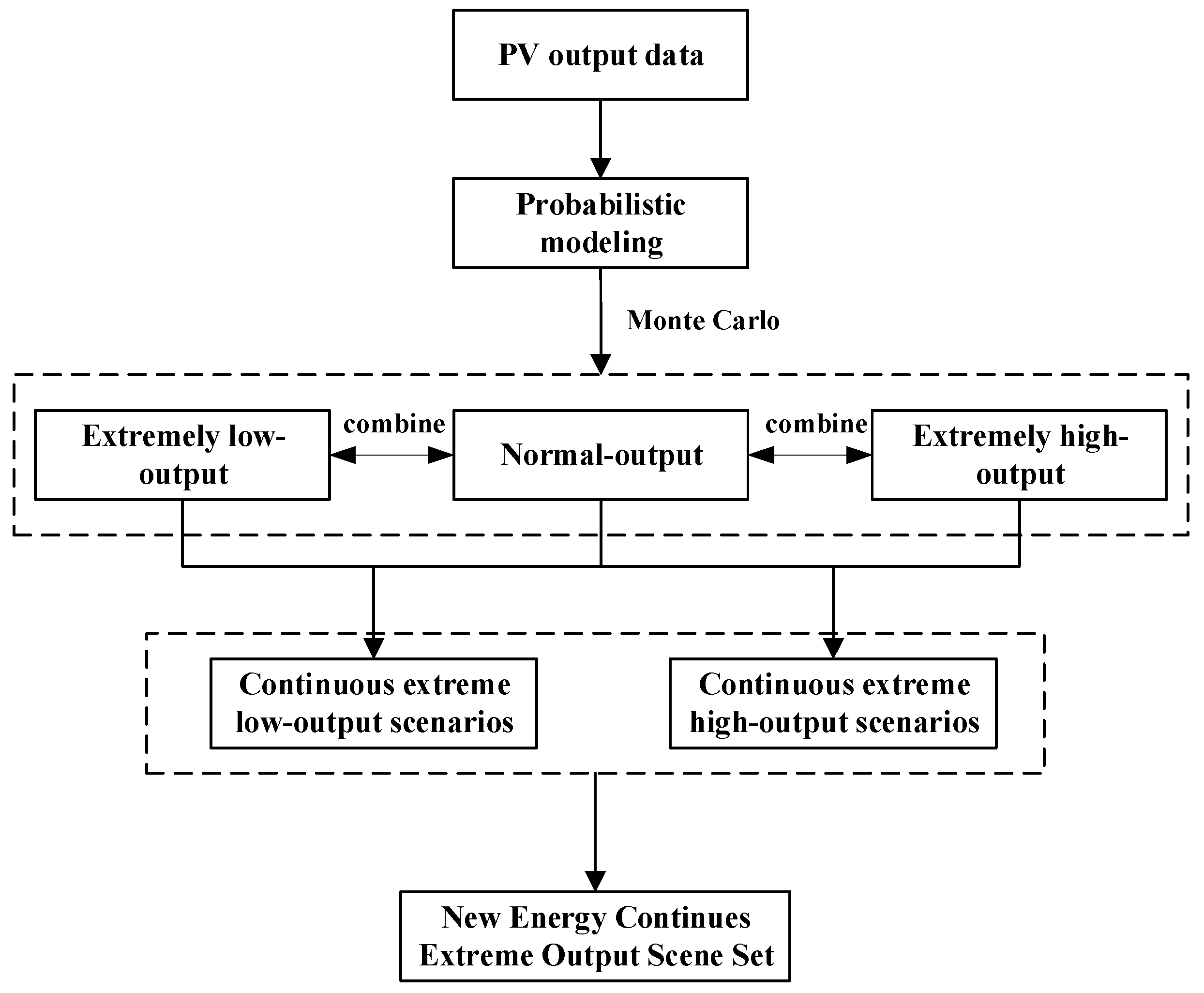
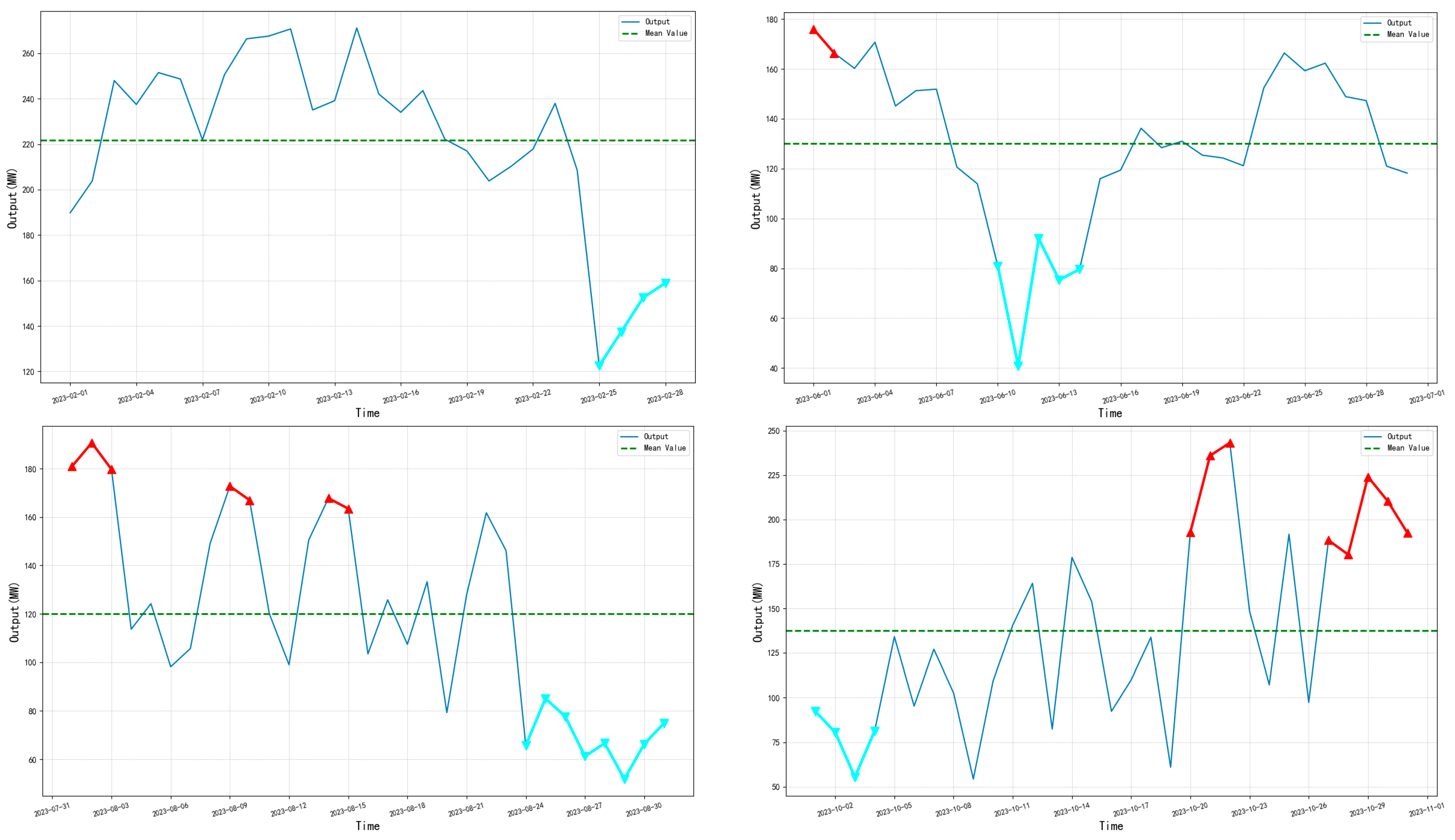
2.1.1. New Energy Continuous Extreme Quantization

To evaluate the impact of renewable energy fluctuations on power supply reliability, when the daily average output of renewables remains below a critical threshold of the monthly average for consecutive days, it is identified as a Continuous Extremely Low-Output Fluctuation. The mathematical formulation is presented in Equation (1). For renewable energy accommodation, when the daily average output continuously exceeds a threshold of the monthly average, it is identified as a Continuous Extremely High-Output Fluctuation, as shown in Equation (2).

$$\left\{P{R}_{\mathrm{t}}\right|P{R}^{ave}-P{R}_{\mathrm{t}}\ge {\epsilon }^{l,\min }P{R}^{ave},\forall t\in {\Gamma }^l,crad({\Gamma }^l)\ge d^{l,\min }\}$$

(1)

$$\left\{P{R}_{\mathrm{t}}\right|P{R}_{\mathrm{t}}-P{R}^{ave}\ge {\epsilon }^{h,\min }P{R}^{ave},\forall t\in {\Gamma }^h,crad({\Gamma }^h)\ge d^{h,\min }\}$$

(2)

where ${PR}_t$ denotes the average renewable output on day $\mathrm{t}$, and $P{R}_{ave}$ represents the monthly average output. The operator $crad\left(·\right)$ denotes the cardinality of a set. The parameters ${\epsilon }^{l,min}$ and $d^{l,min}$ define the characteristics of the continuous extremely low-output scenario, indicating the minimum relative deviation below the monthly average and the minimum duration (in days), respectively. Similarly, ${\epsilon }^{h,min}$ and $d^{h,min}$ are the corresponding parameters for the continuous extremely high-output scenario. These parameters jointly determine the intensity and duration of the extreme output fluctuation scenarios.

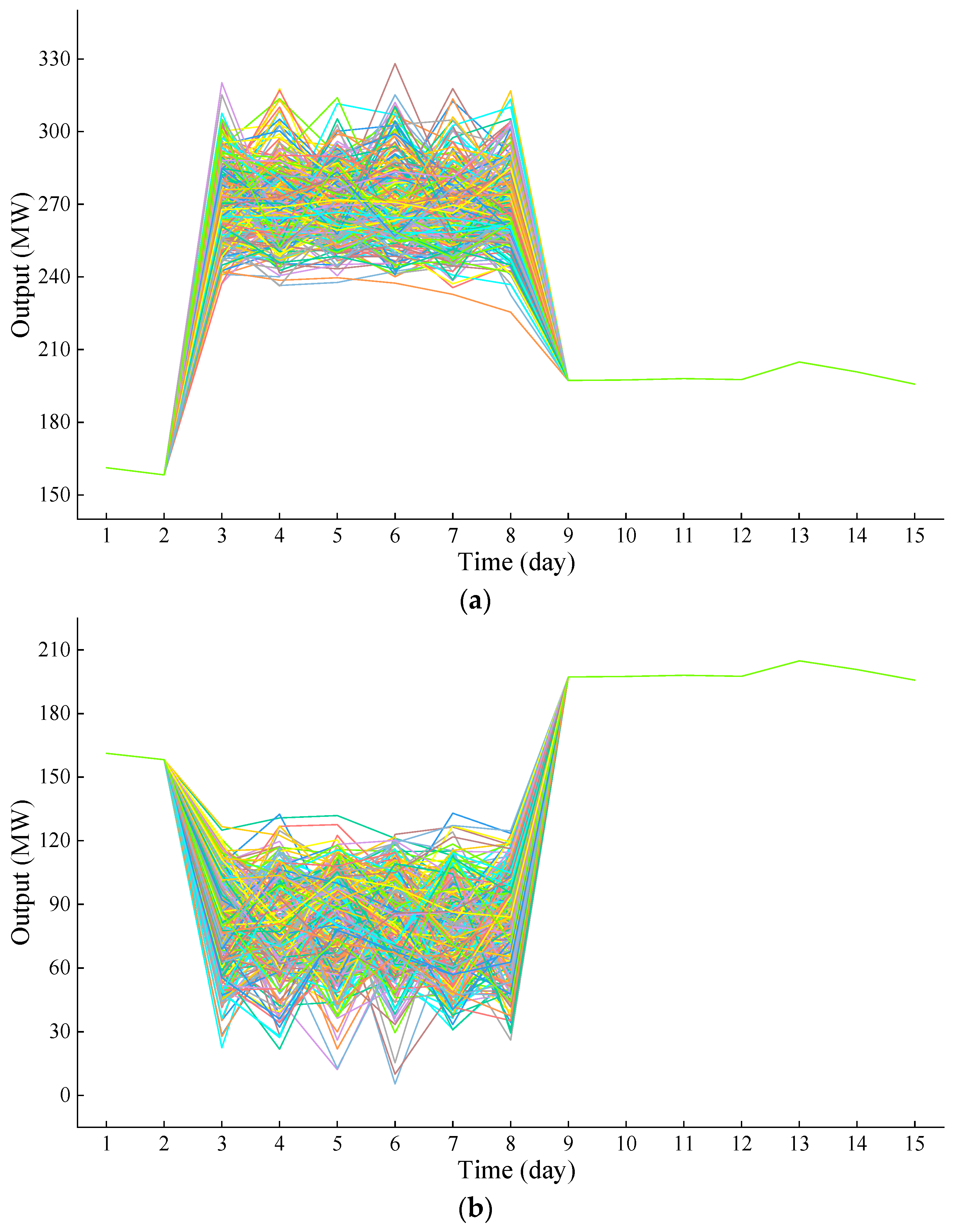
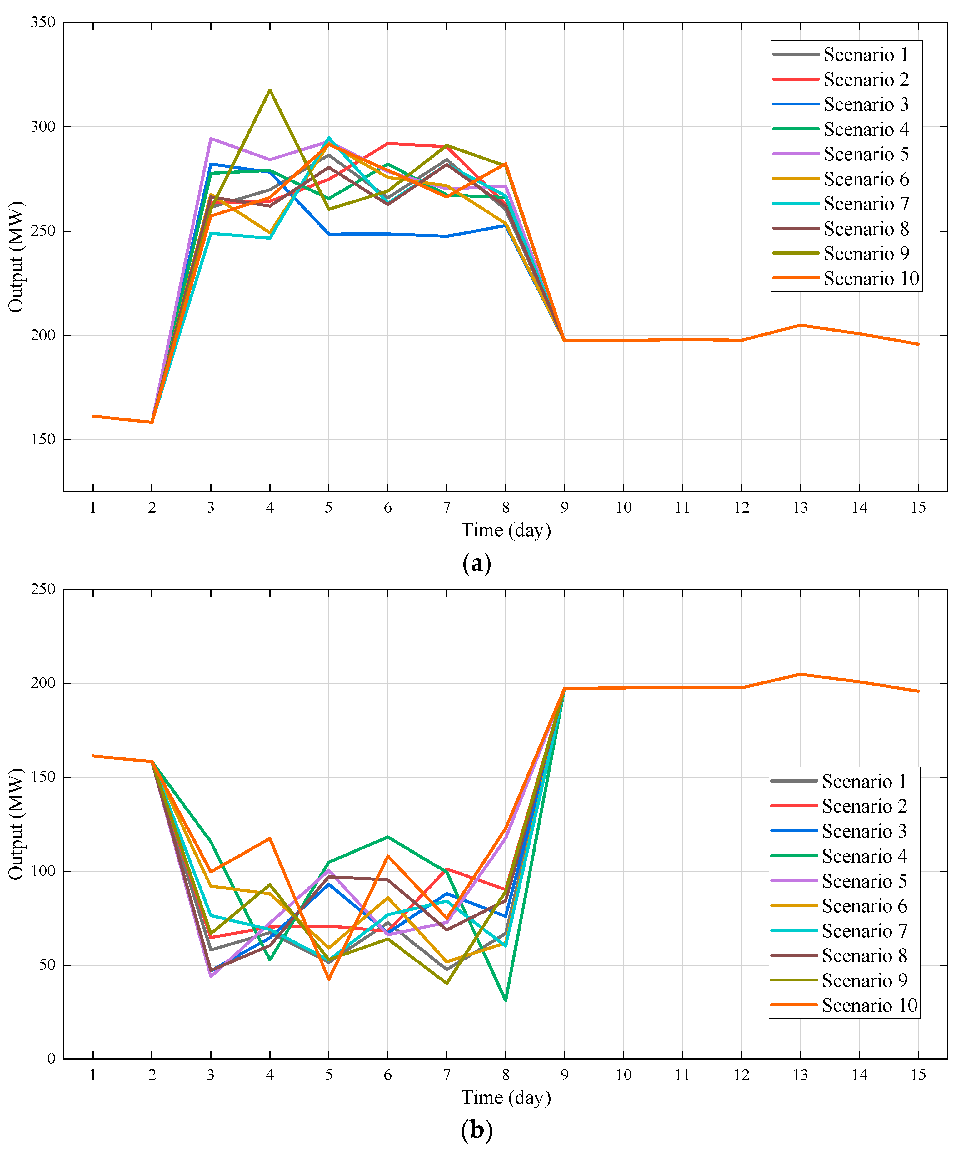
2.1.2. Scenario Generation and Reduction

Accurately quantifying multi-day extreme fluctuations in renewable energy builds a key foundation for implementing optimal scheduling measures. The scenario generation method in this paper consists of three steps (Figure 2):

• Processing historical PV output data to obtain extreme output samples;
• Modeling the probability distribution of the samples using a kernel density function and generating PV output sequences through MC simulation sampling;
• Inserting the extreme sequences into non-extreme sequences to create a scenario set for persistent extreme renewable energy output.

The backward reduction method, specifically, the synchronous backward reduction method, is employed to reduce the large number of extreme scenarios. The specific steps are as follows:

• Initialize the scenario set $S=\{X_1,X_2,\dots ,X_N\}$, where the initial weight of each scenario is $w_i={\displaystyle \frac{1}{N}}$.
• Calculate the distance matrix M for all scenarios using the Wasserstein distance. For N scenarios, the size of the distance matrix is N × N, and each element represents the distance between scenarios $X_i$ and $X_j$.
• Find the smallest value in the distance matrix M, which indicates the highest similarity between scenarios $X_i$ and $X_j$. Merge these two scenarios into a new one, with the weight equal to the sum of their respective weights, and update the scenario set.
• Repeat Step 3 until the number of scenarios is reduced to the target number N.

2.2. Mid-Term Stochastic Optimization Model

2.2.1. Objective Function

The objective function considers both power generation and the deviation between the planned and actual output. The objective is to ensure that there are power generation benefits while reasonably controlling reservoir water levels. The objective function is as follows:

$$\begin{array}{l}\max E={\displaystyle \sum _{n=1}^N{\displaystyle \sum _{\mathrm{t}=1}^T{E}_{n,t}}}-{\displaystyle \sum _{n=1}^N{\displaystyle \sum _{t=1}^T{\displaystyle \sum _{s=1}^S{\mathrm{Pr}}^s{e}_{n,t,s}}}}\\ e_{n,t,s}=\left|E_{n,t}-E{F}_{n,t,s}\right|\\ E_{n,t}=\left(P_{n,t}^h+P_{n,t}^s\right)\mathrm{\Delta }t\\ E{F}_{n,t,s}=\left(P{F}_{n,t,s}^h+P{F}_{n,t,s}^s\right)\mathrm{\Delta }t\end{array}$$

(3)

where $E_{n,t}$ represents the total power generation of reservoir n and its connected PV station at time period t (kWh); ${\mathrm{Pr}}^s$ is the probability of scenario s; $e_{n,t,s}$ is the deviation between the planned total power generation and the actual total power generation (kWh); $P_{n,t}^h$ and $P_{n,t}^s$ are the outputs of reservoir n and its connected PV station at time period t (kW); $E{F}_{n,t,s}$ represents the total power generation of reservoir n and its connected PV station (kWh); $P{F}_{n,t,s}^h$ and $P{F}_{n,t,s}^s$ are the output of reservoir n and its connected PV station (kW); $\mathrm{\Delta }t$ represents the time period length; N is the total number of stations; T is the total number of time periods; and S is the total number of wind–solar output scenarios.

2.2.2. Constraints

(1)

The water balance constraints are as follows:

$$\begin{array}{l}{V}_{n,t+1}=V_{n,t}+3600(Q{I}_{n,t}-Q{U}_{n,t})\mathrm{\Delta }t\\ Q{I}_{n,t}=Q{E}_{n,t}+Q{U}_{n-1,t}\\ Q{U}_{n,t}=Q{D}_{n,t}+Q{S}_{n,t}\end{array}$$

(4)

where $V_{n,t+1}$ and $V_{n,t}$ are the storage of reservoir n (in 10,000 m³) at the ending and beginning of time period t under scenario n, respectively (m³); $Q{I}_{n,t}$ is the inflow (m³/s); $Q{U}_{n,t}$ represents the outflow (m³/s); $Q{E}_{n,t}$ represents the segment inflow (m³/s); $Q{D}_{n,t}$ represents the generation flow (m³/s); and $Q{S}_{n,t}$ is the spill flow (m³/s).

(2)

The initial and final water lever limits are as follows:

$$\begin{array}{l}{Z}_{n,1}=Z_n^{start}\\ Z_{n,T+1}=Z_n^{end}\end{array}$$

(5)

where $Z_{n,1}$ and $Z_{n,T+1}$ represent the initial and final water levels (m) of reservoir n during the scheduling period, respectively (m³); $Z_n^{start}$ and $Z_n^{end}$ represent the given initial and final water levels (m), respectively.

(3)

The water level limits are as follows:

$$Z_{n,t}^{\min }\le Z_{n,t}\le Z_{n,t}^{\max }$$

(6)

where $Z_{n,t}^{\min }$ and $Z_{n,t}^{\max }$ are the minimum and maximum reservoir levels (m) of the reservoir n at time t.

(4)

The power generation flow limits are as follows:

$$Q{D}_{n,t}^{\min }\le Q{D}_{n,t}\le Q{D}_{n,t}^{\max }$$

(7)

where $Q{D}_{n,t}$ denotes the power generation flow (m³/s) of reservoir n at time t.

(5)

The discharge flow limits are as follows:

$$Q{U}_{n,t}^{\min }\le Q{U}_{n,t}\le Q{U}_{n,t}^{\max }$$

(8)

where $Q{U}_{n,t}$ denotes the discharge flow (m³/s) of reservoir n at time t.

(6)

The transmission channel limits are as follows:

$$P_{n,t}\le P{C}_n$$

(9)

where $P{C}_n$ denotes the transmission capacity of reservoir n.

(7)

The power output limits are as follows:

$$P_{n,t}^{h\min }\le P_{n,t}^h\le P_{n,t}^{h\max }$$

(10)

$P_{n,t}^h$ denotes the power output (10,000 kW) of reservoir n at time t. $P_{n,t}^{h\min }$ and $P_{n,t}^{h\max }$ are the minimum and maximum power output (10,000 kW), respectively.

(8)

The daily power output variation limits are as follows:

$$\begin{array}{l}{P}_i^{\max }-P_i^{\min }\le \mu P_i^{\min }\\ P_i^{\max }=\underset{t=1,2,\dots ,T}{\max }(P_{n,t}^h+P_{n,t}^w+P_{n,t}^s)\\ P_i^{\min }=\underset{t=1,2,\dots ,T}{\min }(P_{n,t}^h+P_{n,t}^w+P_{n,t}^s)\end{array}$$

(11)

$P_i^{\max }$ and $P_i^{\min }$ are the maximum and minimum daily average power output (MW).

(9)

The deviation constraint between actual and planned water lever is as follows:

$$\left|Z_{n,t}-Z{F}_{n,t,s}\right|\le {\epsilon }_n$$

(12)

$Z{F}_{n,t,s}$ represents the water level (10,000 m) of reservoir n at time t under scenario s. ${\epsilon }_n$ is the allowable deviation between the actual and planned water levels.

(10)

The hydropower generation limits are as follows:

$$h_{n,t}={\displaystyle \frac{Z_{n,t}+Z_{n,t+1}}{2}}-Z{D}_{n,t}-h_{n,t}^{loss}$$

(13)

$$P_{n,t}^h=\phi (Q{D}_{n,t},h_{n,t})$$

(14)

where $h_{n,t}$ denotes the water head (m), and $h_{n,t}^{loss}$ represents the head loss constant (m); $\phi (·)$ indicates the functional relationship between the power output, turbine discharge, and water head.

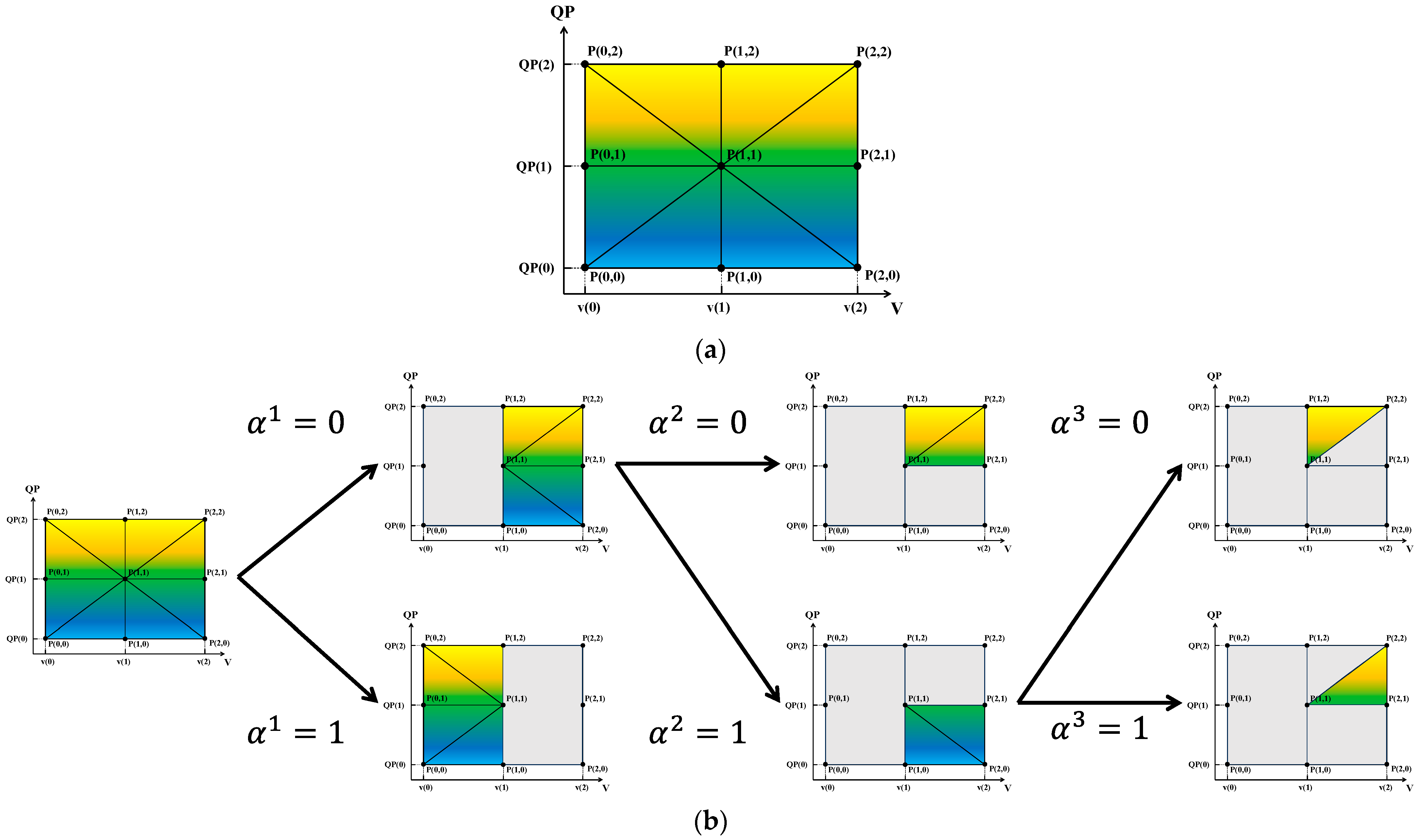
2.2.3. Linearization Method of Nonlinear Constraints

To handle the nonlinear relationship between reservoir storage, turbine discharge, and power output, a three-dimensional piecewise linear approximation method is applied [49]. Based on an independent branching scheme, the nonlinear function is discretized into a 3 × 3 grid with 9 vertices, and the entire surface is further divided into 8 triangular regions, as shown in Figure 3a. Any point located within a triangle can be uniquely determined by the values at its three vertices and the corresponding interpolation weights, as shown in Figure 3b.

Each function value is approximated by convex interpolation over the triangular domain. The corresponding power output is denoted as follows:

$$PH(x,y)=\phi (V(x),QD(y))$$

Three binary 0–1 variables $({\alpha }_1,{\alpha }_2,{\alpha }_3)$ are introduced to identify the triangle in which the current point lies, according to the branching structure. Based on the above modeling approach, the nonlinear equality constraint $PH(x,y)=\phi (V(x),QD(y))$ can be replaced by the liner constants (15)–(21).

$${\displaystyle \sum _x{\displaystyle \sum _y\lambda (x,y)=1}}$$

(15)

$${\displaystyle \sum _y\lambda (0,y)\le {\alpha }_1},{\displaystyle \sum _y\lambda (2,y)\le 1-{\alpha }_1}$$

(16)

$${\displaystyle \sum _x\lambda (x,0)\le {\alpha }_2},{\displaystyle \sum _x\lambda (x,2)\le 1-{\alpha }_2}$$

(17)

$$\lambda (0,1)+\lambda (2,1)\le {\alpha }_3,\lambda (1,0)+\lambda (1,2)\le 1-{\alpha }_3$$

(18)

$$v={\displaystyle \sum _x{\displaystyle \sum _y\lambda (x,y)\cdot V(x)}}$$

(19)

$$q_d={\displaystyle \sum _x{\displaystyle \sum _y\lambda (x,y)\cdot QD(y)}}$$

(20)

$$p_h={\displaystyle \sum _x{\displaystyle \sum _y\lambda (x,y)\cdot PH(x,y)}}$$

(21)

Equation (15) ensures that the interpolation weights of the three vertices of the selected triangle sum to 1. Equations (16)–(18) implement the branch selection mechanism for determining the active triangular region. Equations (19)–(21) perform the linear interpolation of the reservoir storage, turbine discharge, and power output, respectively.

This formulation effectively transforms the nonlinear hydropower conversion model into a set of linear constraints, enabling efficient solutions as a mixed-integer linear program (MILP).

3. Case Study

3.1. Data and Background

This study takes the hydro–solar integrated base in a certain river basin as a case study. In this basin, a key hydropower station serves as a controlling reservoir, playing a crucial role in optimizing hydropower dispatch. This station has multi-year regulation capabilities, allowing it to adjust outputs over different time periods to accommodate stochastic fluctuations in renewable energy generation. With its strong regulation capacity, the hydropower station can mitigate uncertainties in solar power generation through optimized scheduling, ensuring a stable power supply to the grid even during continue fluctuations. Therefore, this study selects this hydropower station as a representative case to analyze its role in hydro–solar complementary optimization and explore hydropower scheduling strategies under high-renewable-energy-penetration scenarios.

For data processing, ERA5 reanalysis data from European Centre for Medium-Range Weather Forecasts (ECMWF) are used for data processing in this study. The data are used to derive historical long-term PV output for the basin and extract extreme output scenarios. The ERA5 dataset, known for its high resolution and global coverage, provides reliable meteorological inputs for renewable energy modeling, enhancing the accuracy and representativeness of PV simulations.

In terms of modeling and solution methodology, the proposed two-stage stochastic optimization scheduling model is implemented in a Python 3.12.4 environment and solved using Gurobi 11.0. Leveraging Gurobi’s powerful solving capabilities, this study optimizes hydro–solar scheduling schemes and verifies the proposed method’s effectiveness in compensating for continuous solar fluctuations.

3.2. Results Analysis

3.2.1. Continuous Extreme Samples

Based on Equations (1) and (2), the cumulative probability distribution curve of historical PV output is derived. To identify periods of continuous extremely low outputs, it is first necessary to define what constitutes an “extreme” event. In this study, the 0.9 quantile of the cumulative distribution curve is selected as the threshold, and days with a PV output below this threshold are considered extreme low-output days. Then, by setting another characterization parameter d = 2, consecutive two-day periods of extremely low outputs are identified and extracted as representative samples for further analysis. Several such samples are illustrated in Figure 4. In the figure, the red solid line represents a continuous extremely high output, while the light blue solid line represents a continuous extremely low output.

3.2.2. Generation of Typical Scenarios

By applying the methods described above to historical PV data, we generated representative extreme-fluctuation scenarios that quantify mid-term PV output uncertainties (Figure 5 and Figure 6).

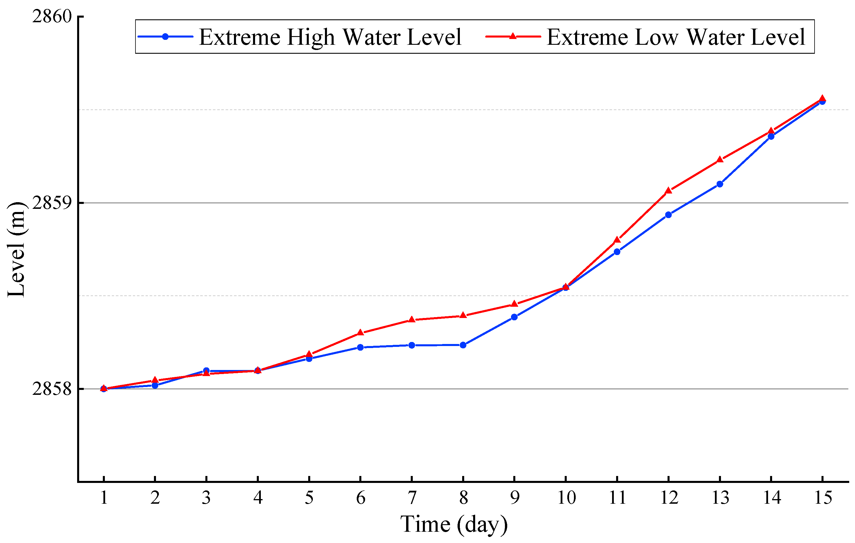
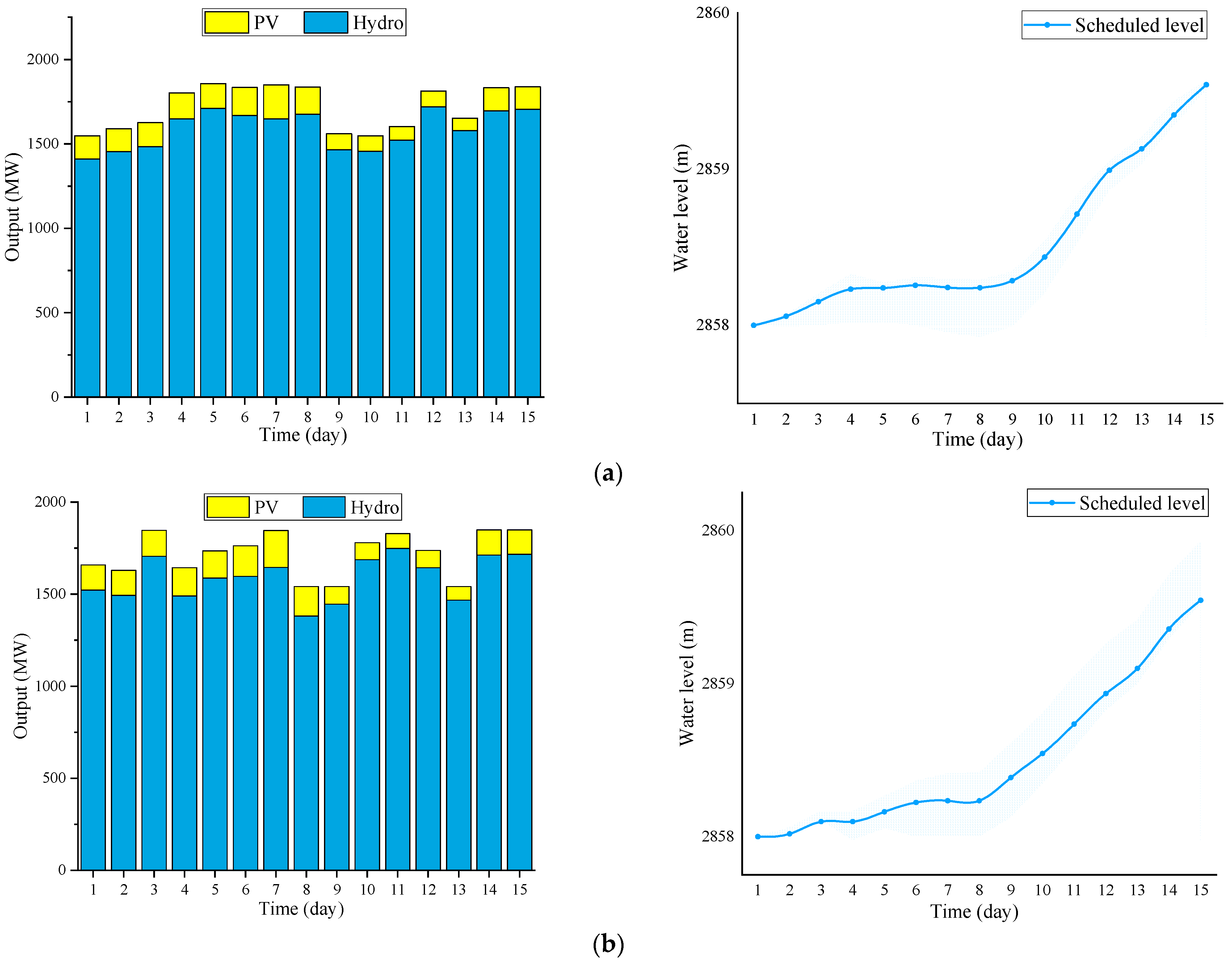
3.2.3. Dispatch Results

The proposed dispatch model was applied to simulate scenarios of consecutive days with extremely high and low PV output. The output process and water level variations of the hydropower stations are shown in Figure 7:

The results demonstrate that the station’s output process is smooth, with minimal daily output fluctuations, closely resembling actual operational conditions. On the water level process chart, the blue-shaded areas represent the water level operating range under extreme PV fluctuation scenarios. It can be observed that the water level fluctuation range is relatively small. This indicates that, based on the established water level trajectory, minor adjustments to the water level can effectively compensate for sustained extreme PV output fluctuations.

Furthermore, compared to scenarios of sustained low PV outputs, the upward water level fluctuations are more pronounced under sustained high PV outputs, while the downward fluctuations are less significant. This finding confirms that the model can effectively address extreme renewable energy fluctuations over the following 15 days.

The water level variations under both extreme scenarios are illustrated in Figure 8. The blue shaded areas represent the fluctuation range of power station water levels under different operational scenarios.

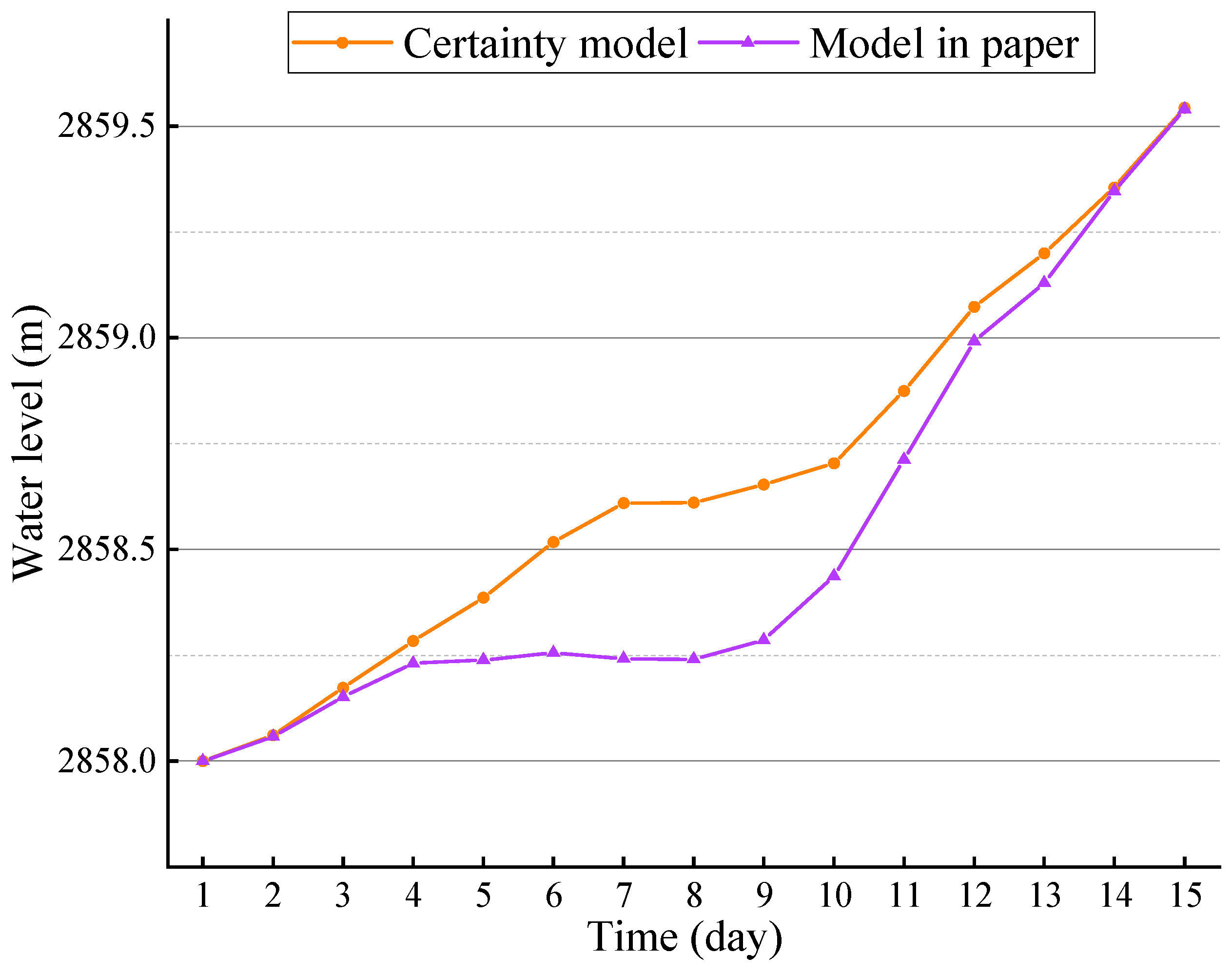
3.2.4. Model Comparison

To verify the effectiveness and superiority of the proposed method, the extremely low-PV-output scenario was used as an example. A deterministic model, which does not consider PV output fluctuations, was compared with the stochastic dispatch model proposed in this study. The total power generation, spilled water volume, and daily water level variations corresponding to the two models are presented in Figure 9 and

Table 1. Comparison of optimization results between certainty model and model in paper.

Indicator	Certainty Model	Model in Paper (High Output)	Model in Paper (Low Output)
Generation	42.09 × 108 kWh	42.09 × 108 kWh	41.24 × 108 kWh
Nonpower release	4.63 × 108 m3	4.69 × 108 m3	5.14 × 108 m3

.

Under the proposed model, considering the sustained extremely low-PV-output scenario, the water level trajectory achieves compensation adjustments for the PV output, with minimal fluctuation. The total power generation is comparable to that of the conventional deterministic model, with no water spillage occurring.

3.2.5. Sensitivity Analysis

To evaluate the sensitivity of the proposed model to inflow variability, a series of runoff scenarios were created by applying ±10%, ±20%, ±30%, and ±40% perturbations to the baseline inflow data. Three representative renewable energy scenarios are considered: (1) continuous extremely high renewable energy output, (2) continuous extremely low renewable energy output, and (3) a deterministic benchmark model without renewable variability.

Under each inflow condition, system performance is assessed across three dimensions: total power generation, water spillage, and reservoir water level volatility. Notably, water level volatility is defined as the deviation of actual reservoir levels from the target level during sustained extreme renewable fluctuations, indicating operational stability.

Table 2. Comparison of modeled power system operating parameters under different runoff conditions (Output: ×10⁸ kWh; Spillage: ×10⁸ m³).

Runoff	High PV Output			Low PV Output			Certainty Model
	Output	Spillage	Volatility	Output	Spillage	Volatility	Output	Spillage	Volatility
−40%	32.91	0.57	0	31.82	0	0.62	32.9	0	6.76
−30%	37.36	0.59	1.66	36.43	0	4.01	37.95	0	9.34
−20%	40.79	1.08	19.55	39.92	0.44	17.09	41.06	0.42	30.07
−10%	41.69	2.84	6.83	41.11	2.26	11.1	41.97	2.33	30.98
Normal	42.09	5.14	13.57	41.24	4.69	8.41	42.09	4.63	13.93
+10%	41.85	7.51	13.67	40.91	6.94	11.73	41.71	6.93	43.6
+20%	42.03	10	3.14	40.92	9.26	23.59	42.03	9.28	26.52
+30%	41.89	12.3	8.21	40.9	11.64	19.29	42	11.71	54.12
+40%	41.98	14.61	5.15	40.87	14	19.19	41.96	14.15	40.32

presents comparative results under all scenarios. Key observations include the following:

The total generation increases with inflow across all scenarios due to enhanced hydropower availability: the extremely high-output scenario maintains marginally higher generation by reducing hydropower regulation demand; the extremely low-output scenario suffers from constrained outputs during water scarcity despite compensation needs, while the deterministic model achieves comparable/higher generation by ignoring renewable fluctuations.

Regarding water spillage and reservoir water level volatility, distinct patterns emerge across the three scenarios. In the extremely high-renewable-output scenario, hydropower generation is frequently suppressed to accommodate the abundant renewable supply, leading to a significant increase in water spillage, especially under high-inflow conditions. Conversely, in the extremely low-output scenario, the greater utilization of available water for electricity generation reduces the likelihood of spillage, resulting in lower spill volumes across most runoff scenarios. The deterministic model exhibits a spillage pattern broadly like that of the high-output scenario, and in some cases, even exceeds it. In terms of reservoir water level volatility, the deterministic model shows the largest fluctuations among the three.

4. Discussion

The core principle of hydro–wind–solar complementary operation is as follows: when the renewable energy output is high, hydropower reduces generation and stores water to reserve regulation capacity; when the renewable output is low, hydropower releases stored energy to compensate and ensure supply reliability. In this process, the reservoir water level directly affects the regulation capability of hydropower stations and is thus critical to both renewable integration and power supply security. This study proposes a mid-term scheduling approach that incorporates sustained extreme fluctuations in renewables into hydropower dispatch. By dynamically optimizing the water level trajectory, the method guides more reasonable reservoir operations, ensuring that there will be sufficient regulation margins and dispatchable capacity in the future.

Unlike most studies that rely on deterministic or overly simplified stochastic assumptions, this work addresses the unpredictability of mid-term wind and solar power by proposing a scenario generation method for sustained extreme fluctuations. Based on this, a mid-term stochastic dispatch model is developed, leveraging hydropower’s flexibility to mitigate renewable output deviations.

This study focuses only on sustained extreme fluctuations in wind and solar output, without considering hydrological extremes such as floods or droughts. The analysis is limited to the basin scale. Broader applications would require the consideration of transmission constraints, market mechanisms, and multi-stakeholder coordination. Currently, wind power is not included, and extreme scenarios are generated solely from historical output distributions, which may not capture future extremes. Future work could integrate climate features and use machine learning—such as neural networks—to better model weather-driven renewable variability.

Future work could introduce stochastic modeling and adopt a robust–stochastic hybrid optimization strategy to enhance the robustness of power generation. This approach would ensure safety constraints under extreme worst-case scenarios while maintaining economic efficiency in typical or average conditions, thereby achieving a dynamic balance between robust reliability and stochastic economic performance.

5. Conclusions

The proposed two-stage stochastic optimization model effectively addresses the challenge of sustained extreme fluctuations in renewable energy within multi-energy complementary systems. It ensures that hydropower reservoirs maintain sufficient flexibility—in terms of both water storage and discharge—to handle continuous periods of high or low renewable energy outputs. This improves generation benefits and enables the stable regulation of water levels across stations.

The scenario generation and reduction method efficiently capture high-frequency extreme events, enhancing the computational efficiency while preserving critical system behavior. Compared to traditional deterministic approaches, the model provides stronger renewable energy compensation and greater operational stability, particularly under extreme conditions, without compromising the total power generation or increasing water spillage. Sensitivity analysis confirms that the model significantly reduces water level fluctuations under uncertain inflows, underscoring its robustness and reliability in long-term scheduling under extreme renewable energy variability.

References

- Tong, D.; Zhang, Q.; Zheng, Y.; Caldeira, K.; Shearer, C.; Hong, C.; Qin, Y.; Davis, S.J. Committed emissions from existing energy infrastructure jeopardize 1.5 °C climate target. Nature 2019, 572, 373–377. [Google Scholar] [CrossRef] [PubMed]
- Osman, A.I.; Nasr, M.; Eltaweil, A.S.; Hosny, M.; Farghali, M.; Al-Fatesh, A.S.; Rooney, D.W.; Abd El-Monaem, E.M. Advances in hydrogen storage materials: Harnessing innovative technology, from machine learning to computational chemistry, for energy storage solutions. Int. J. Hydrogen Energy 2024, 67, 1270–1294. [Google Scholar] [CrossRef]
- Matevosyan, J.; Olsson, M.; Söder, L. Hydropower planning coordinated with wind power in areas with congestion problems for trading on the spot and the regulating market. Electr. Power Syst. Res. 2009, 79, 39–48. [Google Scholar] [CrossRef]
- Huh, S.-Y.; Lee, J.; Shin, J. The economic value of South Korea׳s renewable energy policies (RPS, RFS, and RHO): A contingent valuation study. Renew. Sustain. Energy Rev. 2015, 50, 64–72. [Google Scholar] [CrossRef]
- Omri, A.; Ben Jabeur, S. Climate policies and legislation for renewable energy transition: The roles of financial sector and political institutions. Technol. Forecast. Soc. Change 2024, 203, 123347. [Google Scholar] [CrossRef]
- Shang, Y.; Sang, S.; Tiwari, A.K.; Khan, S.; Zhao, X. Impacts of renewable energy on climate risk: A global perspective for energy transition in a climate adaptation framework. Appl. Energy 2024, 362, 122994. [Google Scholar] [CrossRef]
- Bolan, S.; Padhye, L.P.; Jasemizad, T.; Govarthanan, M.; Karmegam, N.; Wijesekara, H.; Amarasiri, D.; Hou, D.; Zhou, P.; Biswal, B.K.; et al. Impacts of climate change on the fate of contaminants through extreme weather events. Sci. Total Environ. 2024, 909, 168388. [Google Scholar] [CrossRef]
- Li, H.; Ren, Z.; Fan, M.; Li, W.; Xu, Y.; Jiang, Y.; Xia, W. A review of scenario analysis methods in planning and operation of modern power systems: Methodologies, applications, and challenges. Electr. Power Syst. Res. 2022, 205, 107722. [Google Scholar] [CrossRef]
- Panigrahi, R.; Mishra, S.K.; Srivastava, S.C.; Srivastava, A.K.; Schulz, N.N. Grid Integration of Small-Scale Photovoltaic Systems in Secondary Distribution Network—A Review. IEEE Trans. Ind. Appl. 2020, 56, 3178–3195. [Google Scholar] [CrossRef]
- Liu, H.; Wang, C.; Ju, P.; Li, H. A sequentially preventive model enhancing power system resilience against extreme-weather-triggered failures. Renew. Sustain. Energy Rev. 2022, 156, 111945. [Google Scholar] [CrossRef]
- Ren, Y.; Sun, K.; Zhang, K.; Han, Y.; Zhang, H.; Wang, M.; Jing, X.; Mo, J.; Zou, W.; Xing, X. Optimization of the capacity configuration of an abandoned mine pumped storage/wind/photovoltaic integrated system. Appl. Energy 2024, 374, 124089. [Google Scholar] [CrossRef]
- Xiaorong, X.; Ningjia, M.; Wei, L.; Wei, Z.; Peng, X.; Haozhi, L. Functions of Energy Storage in Renewable Energy Dominated Power Systems. Proc. CSEE 2023, 43, 158–169. [Google Scholar] [CrossRef]
- Olabi, A.G.; Onumaegbu, C.; Wilberforce, T.; Ramadan, M.; Abdelkareem, M.A.; Al-Alami, A.H. Critical review of energy storage systems. Energy 2021, 214, 118987. [Google Scholar] [CrossRef]
- Dong, Z.; Zhang, Z.; Huang, M.; Yang, S.; Zhu, J.; Zhang, M.; Chen, D. Research on day-ahead optimal dispatching of virtual power plants considering the coordinated operation of diverse flexible loads and new energy. Energy 2024, 297, 131235. [Google Scholar] [CrossRef]
- Zhou, Y.; Zhu, Y.; Luo, Q.; Wei, Y.; Mei, Y.; Chang, F.-J. Optimizing pumped-storage power station operation for boosting power grid absorbability to renewable energy. Energy Convers. Manag. 2024, 299, 117827. [Google Scholar] [CrossRef]
- Yu, S.; Zhou, S.; Chen, N. Multi-objective optimization of capacity and technology selection for provincial energy storage in China: The effects of peak-shifting and valley-filling. Appl. Energy 2024, 355, 122289. [Google Scholar] [CrossRef]
- Zhao, J.; Feng, X.; Pang, Q.; Fowler, M.; Lian, Y.; Ouyang, M.; Burke, A.F. Battery safety: Machine learning-based prognostics. Prog. Energy Combust. Sci. 2024, 102, 101142. [Google Scholar] [CrossRef]
- Kumar, R.; Lee, D.; Ağbulut, Ü.; Kumar, S.; Thapa, S.; Thakur, A.; Jilte, R.D.; Saleel, C.A.; Shaik, S. Different energy storage techniques: Recent advancements, applications, limitations, and efficient utilization of sustainable energy. J. Therm. Anal. Calorim. 2024, 149, 1895–1933. [Google Scholar] [CrossRef]
- Guo, Y.; Ming, B.; Huang, Q.; Wang, Y.; Zheng, X.; Zhang, W. Risk-averse day-ahead generation scheduling of hydro–wind–photovoltaic complementary systems considering the steady requirement of power delivery. Appl. Energy 2022, 309, 118467. [Google Scholar] [CrossRef]
- Jiang, J.; Ming, B.; Huang, Q.; Chang, J.; Liu, P.; Zhang, W.; Ren, K. Hybrid generation of renewables increases the energy system’s robustness in a changing climate. J. Clean. Prod. 2021, 324, 129205. [Google Scholar] [CrossRef]
- Zhu, F.; Zhong, P.-a.; Xu, B.; Liu, W.; Wang, W.; Sun, Y.; Chen, J.; Li, J. Short-term stochastic optimization of a hydro-wind-photovoltaic hybrid system under multiple uncertainties. Energy Convers. Manag. 2020, 214, 112902. [Google Scholar] [CrossRef]
- Jurasz, J.; Canales, F.A.; Kies, A.; Guezgouz, M.; Beluco, A. A review on the complementarity of renewable energy sources: Concept, metrics, application and future research directions. Sol. Energy 2020, 195, 703–724. [Google Scholar] [CrossRef]
- Ma, C.; Liu, L. Optimal capacity configuration of hydro-wind-PV hybrid system and its coordinative operation rules considering the UHV transmission and reservoir operation requirements. Renew. Energy 2022, 198, 637–653. [Google Scholar] [CrossRef]
- Huang, K.; Luo, P.; Liu, P.; Kim, J.S.; Wang, Y.; Xu, W.; Li, H.; Gong, Y. Improving complementarity of a hybrid renewable energy system to meet load demand by using hydropower regulation ability. Energy 2022, 248, 123535. [Google Scholar] [CrossRef]
- Li, Y.; Wang, R.; Li, Y.; Zhang, M.; Long, C. Wind power forecasting considering data privacy protection: A federated deep reinforcement learning approach. Appl. Energy 2023, 329, 120291. [Google Scholar] [CrossRef]
- Fan, Y.; Liu, W.; Zhu, F.; Wang, S.; Yue, H.; Zeng, Y.; Xu, B.; Zhong, P.-A. Short-term stochastic multi-objective optimization scheduling of wind-solar-hydro hybrid system considering source-load uncertainties. Appl. Energy 2024, 372, 123781. [Google Scholar] [CrossRef]
- Zhang, Z.; Dai, H.; Jiang, D.; Yu, Y. Multi-objective operation rule optimization of wind-solar-hydro hybrid power system based on knowledge graph structure. J. Clean. Prod. 2025, 486, 144514. [Google Scholar] [CrossRef]
- Qiu, L.; He, L.; Lu, H.; Liang, D. Systematic potential analysis on renewable energy centralized co-development at high altitude: A case study in Qinghai-Tibet plateau. Energy Convers. Manag. 2022, 267, 115879. [Google Scholar] [CrossRef]
- Almaraashi, M.; Abdulrahim, M.; Hagras, H. A Life-Long Learning XAI Metaheuristic-Based Type-2 Fuzzy System for Solar Radiation Modeling. IEEE Trans. Fuzzy Syst. 2024, 32, 2102–2115. [Google Scholar] [CrossRef]
- Shen, F.; Zhao, L.; Du, W.; Zhong, W.; Peng, X.; Qian, F. Data-Driven Stochastic Robust Optimization for Industrial Energy System Considering Renewable Energy Penetration. ACS Sustain. Chem. Eng. 2022, 10, 3690–3703. [Google Scholar] [CrossRef]
- Yan, R.; Wang, J.; Huo, S.; Qin, Y.; Zhang, J.; Tang, S.; Wang, Y.; Liu, Y.; Zhou, L. Flexibility improvement and stochastic multi-scenario hybrid optimization for an integrated energy system with high-proportion renewable energy. Energy 2023, 263, 125779. [Google Scholar] [CrossRef]
- Shi, Y.; Wang, H.; Li, C.; Negnevitsky, M.; Wang, X. Stochastic optimization of system configurations and operation of hybrid cascade hydro-wind-photovoltaic with battery for uncertain medium- and long-term load growth. Appl. Energy 2024, 364, 123127. [Google Scholar] [CrossRef]
- Li, J.; Zhou, J.; Chen, B. Review of wind power scenario generation methods for optimal operation of renewable energy systems. Appl. Energy 2020, 280, 115992. [Google Scholar] [CrossRef]
- Lucheroni, C.; Boland, J.; Ragno, C. Scenario generation and probabilistic forecasting analysis of spatio-temporal wind speed series with multivariate autoregressive volatility models. Appl. Energy 2019, 239, 1226–1241. [Google Scholar] [CrossRef]
- Li, J.; Zhu, D. Combination of moment-matching, Cholesky and clustering methods to approximate discrete probability distribution of multiple wind farms. IET Renew. Power Gener. 2016, 10, 1450–1458. [Google Scholar] [CrossRef]
- Ioannou, A.; Fuzuli, G.; Brennan, F.; Yudha, S.W.; Angus, A. Multi-stage stochastic optimization framework for power generation system planning integrating hybrid uncertainty modelling. Energy Econ. 2019, 80, 760–776. [Google Scholar] [CrossRef]
- Ren, Z.; Li, W.; Billinton, R.; Yan, W. Probabilistic Power Flow Analysis Based on the Stochastic Response Surface Method. IEEE Trans. Power Syst. 2016, 31, 2307–2315. [Google Scholar] [CrossRef]
- Al-Duais, F.S.; Al-Sharpi, R.S. A unique Markov chain Monte Carlo method for forecasting wind power utilizing time series model. Alex. Eng. J. 2023, 74, 51–63. [Google Scholar] [CrossRef]
- Chen, J.; Rabiti, C. Synthetic wind speed scenarios generation for probabilistic analysis of hybrid energy systems. Energy 2017, 120, 507–517. [Google Scholar] [CrossRef]
- Jiang, C.; Mao, Y.; Chai, Y.; Yu, M.; Tao, S. Scenario Generation for Wind Power Using Improved Generative Adversarial Networks. IEEE Access 2018, 6, 62193–62203. [Google Scholar] [CrossRef]
- Ding, Z.; Wen, X.; Tan, Q.; Yang, T.; Fang, G.; Lei, X.; Zhang, Y.; Wang, H. A forecast-driven decision-making model for long-term operation of a hydro-wind-photovoltaic hybrid system. Appl. Energy 2021, 291, 119353. [Google Scholar] [CrossRef]
- Li, H.; Liu, P.; Guo, S.; Ming, B.; Cheng, L.; Yang, Z. Long-term complementary operation of a large-scale hydro-photovoltaic hybrid power plant using explicit stochastic optimization. Appl. Energy 2019, 238, 863–875. [Google Scholar] [CrossRef]
- Xu, S.; Liu, P.; Li, X.; Cheng, Q.; Liu, Z. Deriving long-term operating rules of the hydro-wind-PV hybrid energy system considering electricity price. Renew. Energy 2023, 219, 119353. [Google Scholar] [CrossRef]
- Lu, N.; Wang, G.; Su, C.; Ren, Z.; Peng, X.; Sui, Q. Medium- and long-term interval optimal scheduling of cascade hydropower-photovoltaic complementary systems considering multiple uncertainties. Appl. Energy 2024, 353, 122085. [Google Scholar] [CrossRef]
- Zhao, Z.; Yu, Z.; Kang, Y.; Wang, J.; Cheng, C.; Su, H. Hydro-photovoltaic complementary dispatch based on active regulation of cascade hydropower considering multi-transmission channel constraints. Appl. Energy 2025, 377, 124573. [Google Scholar] [CrossRef]
- Fang, Y.; Han, J.; Du, E.; Jiang, H.; Fang, Y.; Zhang, N.; Kang, C. Electric energy system planning considering chronological renewable generation variability and uncertainty. Appl. Energy 2024, 373, 123961. [Google Scholar] [CrossRef]
- Guo, L.; Liu, S.; Xi, L.; Zhang, G.; Liu, Z.; Zeng, Q.; Lü, F.; Wang, Y. Research on the Short-Term Economic Dispatch Method of Power System Involving a Hydropower-Photovoltaic-Pumped Storage Plant. Electronics 2024, 13, 1282. [Google Scholar] [CrossRef]
- Liu, Y.; Zhang, H.; Guo, P.; Wu, S. Short-term complementary scheduling of cascade energy storage systems for wind and solar regulation. J. Energy Storage 2025, 124, 116775. [Google Scholar] [CrossRef]
- Zhang, J.; Cheng, C.; Yu, S.; Su, H. Chance-constrained co-optimization for day-ahead generation and reserve scheduling of cascade hydropower–variable renewable energy hybrid systems. Appl. Energy 2022, 324, 119732. [Google Scholar] [CrossRef]