Hybrid Multi-Branch Attention–CNN–BiLSTM Forecast Model for Reservoir Capacities of Pumped Storage Hydropower Plant

Abstract

Pumped storage hydropower plants are important resources for scheduling urban energy storage, which realize the conversion of electric energy through upper and lower reservoir capacities. Dynamic forecasting of reservoir capacities is crucial for scheduling pumped storage and maximizing the economic benefits of pumped storage hydropower plants. In this work, a hybrid forecast network is proposed for both the upper and lower reservoir capacities of a pumped storage hydropower plant. A bidirectional long- and short-term memory network (BiLSTM) is designed as the baseline for the prediction model. A convolutional neural network (CNN) and Squeeze-and-Excitation (SE) attention mechanism are designed to extract local features from raw time series data to capture short-term dependencies. In order to better distinguish the effects of different data types on the reservoir capacity, the correlation between data and reservoir capacity is analyzed using the Spearman coefficient, and a multi-branch forecast model is established based on the correlation. A fusion module is designed to weight and fuse the branch prediction results to obtain the final reservoir capacities forecast model, namely, Multi-Branch Attention–CNN–BiLSTM. The experimental results show that the proposed model exhibits better forecast accuracy in forecasting the reservoir capacity compared with existing methods. Compared with BiLSTM, the $MAPE$ of the forecast values of the reservoir capacities of the upper and lower reservoirs decreased by $1.93\%$ and $2.2484\%$, the $RMSE$ decreased by $16.9887{\mathrm{m}}^3$ and $14.2903{\mathrm{m}}^3$, and the $R^2$ increased by $0.1278$ and $0.1276$, respectively.

1. Introduction

Among existing large-scale energy storage technologies, pumped storage power plants are the most attractive large-scale energy storage solution, due to the vast potential energy contained in their reservoirs, the high full-cycle energy conversion efficiency, the low unit cost of generation, and the flexibility they provide to transmission system operators in short-term operations [1]. Pumped storage hydropower plants are important energy storage resources in the power system, which realize the recovery of electricity by mobilizing the water volume in reservoirs [2,3]. The main components of a pumped storage system include an upper reservoir (UR) and a lower reservoir (LR) for water storage, pressure pipes connecting the UR and LR, and pumps to lift water from the lower reservoir to the upper reservoir [4]. Reservoir capacity is a core parameter of pumped storage hydropower plant operation, in which the upper reservoir is responsible for storing potential energy and the lower reservoir is used to collect the returning water. 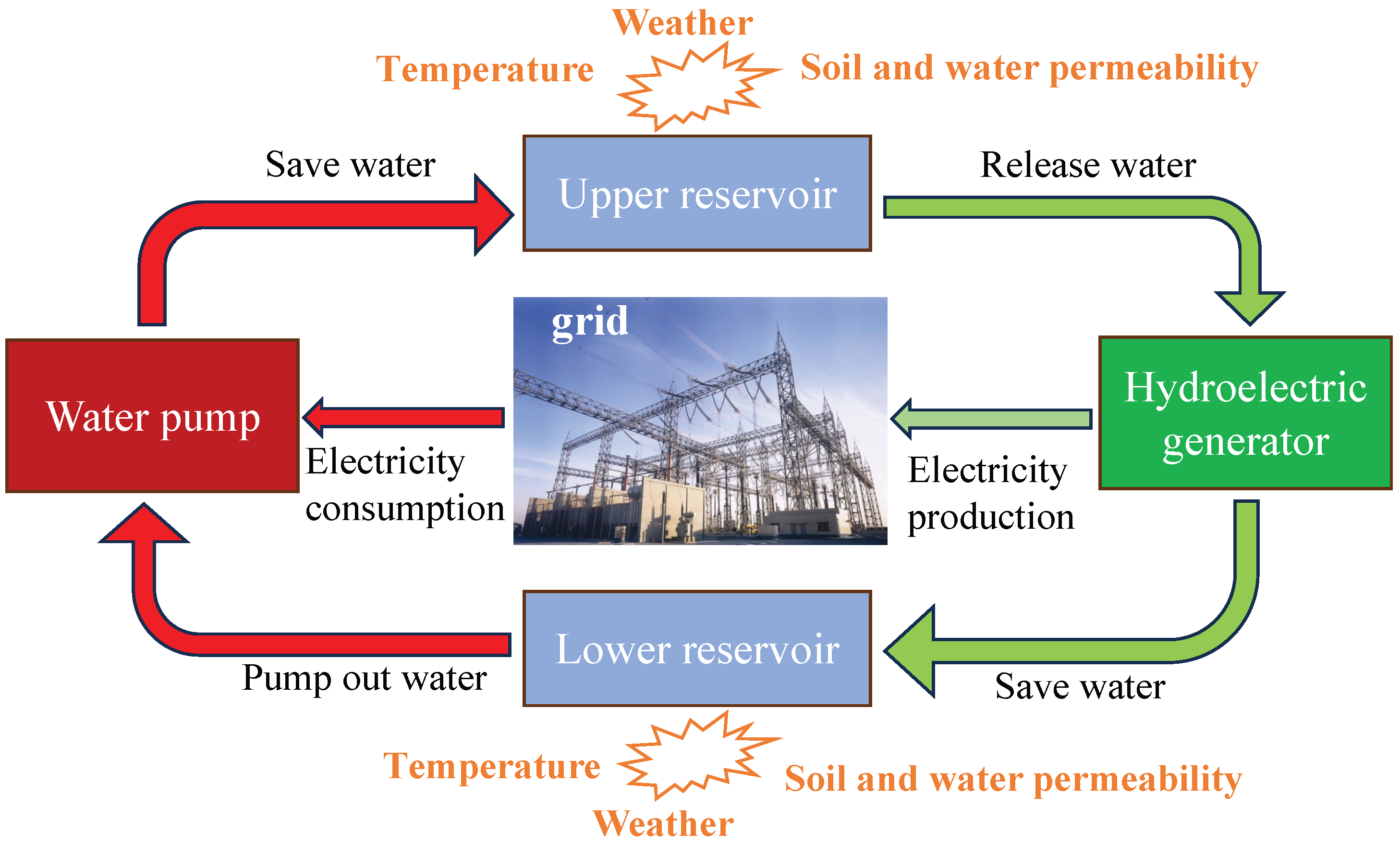The capacity determines the energy storage capacity and operation efficiency of the pumping station [5]. By using the electric power for pumping at the low point of electricity consumption, the water is stored in the upper reservoir, and releasing the water generates electricity at the peak point of electricity consumption. Pumped storage hydropower plants can provide the grid with functions such as peak shifting, valley filling, and emergency backup [6]. A schematic of a pumped storage hydropower plant is shown in Figure 1. The reservoir capacities are affected by many factors, including the released/saved water, weather, temperature, and soil and water permeability. Pumped storage accounts for approximately 96% of global stored electricity capacity and 99% of global stored energy [7]. An accurate forecast of upper and lower reservoir capacity changes is important for realizing efficient scheduling and safe pumping station operation. The accurate forecasting of reservoir capacity can not only optimize the scheduling strategy of a pumping station but also reasonably allocate the water scheduling of the upper and lower reservoirs, improving the overall energy efficiency of pumping station operation. Therefore, the combination of advanced data-driven forecast methods can comprehensively explore the complex nonlinear relationship between multiple variables and provide a scientific basis for decision makers, which effectively guarantees the efficient and sustainable operation of pumped storage hydropower plants.

Data correlation analysis is a statistical method used to assess relationships between variables and is widely used in scientific research and practical decision-making [2]. The correlation between input data and output data needs to be considered when making predictive models, and data with higher correlation can improve the predictive accuracy of the model. Common methods include the Pearson correlation coefficient [8], Spearman correlation coefficient [9], and Kendall correlation coefficient [10]. The Pearson correlation coefficient is used to measure the linear relationship between two continuous variables and is suitable for data that are normally distributed and linear [11]. The Spearman correlation coefficient and the Kendall correlation coefficient are based on the ordering of the data and are able to capture nonlinear but monotonic relationships and are suitable for the analysis of data that have a high number of outliers or are not normally distributed [12]. The development of prediction models has experienced a gradual evolution from traditional statistical methods to modern deep learning models [13]. Traditional mathematical models such as linear regression [14], autoregressive (AR) analysis [15], and the differential autoregressive moving average (ARMA) [16] are widely used because of their simplicity and efficiency. However, these methods have limited ability to portray nonlinear features and complex relationships [17]. Subsequently, Support Vector Regression (SVR) [18] and Random Forest (RF) [19], based on integrated learning and gradient-boosted decision trees [20], have emerged, enhancing the ability of modeling nonlinear relationships but performing slightly less well in capturing time dependencies.

With the development of neural networks, such as back-propagation neural networks (BPNNs) [21] and artificial neural networks (ANNs) [22], the ability of models to recognize complex nonlinear features is further improved [23]. In particular, deep learning models such as convolutional neural networks (CNNs) [24,25,26,27] and long short-term memory (LSTM) networks [28,29] have gradually become mainstream, with CNNs being able to efficiently extract local features and LSTM being effective at capturing long-term and short-term temporal dependencies. LSTM effectively solves the problem of gradient vanishing in traditional recurrent neural networks (RNNs) in long sequence learning through its gating mechanism, while bidirectional LSTM (BiLSTM) further develops this structure to capture richer contextual information in the time series by simultaneously processing the sequence data in both the forward and backward directions [30], thus improving the comprehensiveness and accuracy of prediction [31]. In order to obtain more accurate prediction models, hybrid models combining CNNs with LSTM or BiLSTM are widely used, which significantly improve the prediction accuracy by integrating the advantages of CNNs and LSTM [32]. The pattern of partial discharge for overhead covered conductors is detected by combing LSTM and GRUs together [33].

To further enhance the model’s ability to focus on key features, researchers introduced an attention mechanism to dynamically adjust the feature channel weights in a prediction model. The attention mechanism was implemented mainly by assigning weights to map the importance of different parts of the input to a weight vector [34]. The common methods for computing attention are mainly dot product attention and additive attention [35]. These methods obtain the weights associated with the input by performing appropriate transformations and similarity calculations on the input features. The Squeeze-and-Excitation (SE) attention mechanism is widely used in CNNs. In recent years, the multi-branch network structure has also received increasing focus [36]. This structure is able to extract the feature representation of each type of information in a targeted way by introducing multiple independent branch networks to specialize different input features.

In order to better manage the scheduling of upper and lower reservoir capacities in pumping stations, this paper establishes a Multi-Branch Attention–CNN–BiLSTM forecast model for predicting upper and lower reservoir capacities at future moments. Specifically, BiLSTM is used as the baseline forecast model, and a CNN is introduced to extract local features from raw time series data to capture short-term dependencies. An SE attention mechanism is used to adaptively adjust the weights of the forecast network. In order to further analyze the relationship between the data, the correlation between the input data and the output data is analyzed by using Spearman’s eigenfactors. A three-branch structure is set up and the branch forecast results are weighted to obtain the final forecast results, forming the Multi-Branch Attention–CNN–BiLSTM network. The main contributions of this paper can be summarized as follows:

(1)

An improved Multi-Branch Attention–CNN–BiLSTM network is proposed for reservoir capacity forecasting to improve feature extraction ability and enhance accuracy. A weighted fusion module is proposed to fuse the forecasting results. The proposed Multi-Branch Attention–CNN–BiLSTM framework can better capture nonlinear and non-stationary features of the data samples.

(2)

Spearman’s coefficient is presented to analyze the input–output data relationship to optimize feature selection and focus on the most relevant features. SE is designed to adaptively adjust the weights of the network, thereby enhancing the model’s ability to focus on the most relevant features for more accurate forecast.

(3)

A real application validation in a hydropower generation station shows that the proposed model can enhance model robustness and improve accuracy for reservoir capacity forecasting.

The outline of this work is given as follows. Data Descriptions and Pre-Processing is given in Section 2 with details of data descriptions and pre-processing. The Multi-Branch Attention–CNN–BiLSTM model is presented for reservoir capacity forecasting in Section 3. In Section 4, experimental results and analysis are given to show the effectiveness of the proposed method. Section 5 concludes this work.

2. Data Descriptions and Pre-Processing

2.1. Construction of Dataset

In this paper, real-time operational data from January 2023 to May 2023 of a pumped storage hydropower plant were used. The sample time interval is 30 min. The pumping station has an upper reservoir and a lower reservoir, and four speed-regulated pumps are installed in the pipeline connecting the upper and lower reservoirs to accomplish power generation and water transfer operations. The power and speed of each pump can be varied by regulation. The available data include the power and speed of each pump and the water level in the upper and lower reservoirs. Data were collected using sensors and transferred in real time to a database for storage and easy reading. The data types and units are shown in

Table 1. Data types and units.

Data Type	Unit	Data Type	Unit
U01 power	kW	U01 speed	Hz
U02 power	kW	U02 speed	Hz
U03 power	kW	U03 speed	Hz
U04 power	kW	U04 speed	Hz
Upper reservoir level 1	m	Upper reservoir level 2	m
Lower reservoir level 1	m	Lower reservoir level 2	m
Upper reservoir capacity	${\mathrm{m}}^3$	Lower reservoir capacity	${\mathrm{m}}^3$

, where $U01$–$U04$ are the models of the four pumps, and the reservoir levels are represented by 1 and 2 for the upper and lower reservoirs, respectively. Pumps $U01$ and $U03$ are the connecting pumps of the pipeline from the lower reservoir to the upper reservoir for pumping water. Pumps $U02$ and $U04$ are connecting pumps for the pipeline from the lower reservoir to the upper reservoir for power generation. Both the upper and lower reservoir levels are the water level of the reservoir capacity. Reservoir levels 1 and 2 indicate the height of the reservoir level measured by the two sensors. Reservoir capacity indicates the volume of water in the reservoir. The forecasting of the capacities of the upper and lower reservoirs is investigated. The capacity distributions of the upper and lower reservoirs are shown in Figure 2. It can be seen that there is a certain periodicity in the distribution of the upper and lower reservoir capacities.

2.2. Data Pre-Processing

The dataset has some data with large deviations, which are due to errors caused by the sensors. In this paper, simple data processing was carried out on the data to eliminate the data which is beyond the normal range. Due to the excessive amount of data collected, not all of it can be used for reservoir forecasting. In this paper, the feature selection method of the Spearman coefficient was used to select the parameters which are more correlated with the reservoir capacities. The Spearman feature selection coefficient is a statistical measure of the relationship between variables. The Spearman coefficient assesses the correlation of variables by comparing their ranks. Specifically, the features and target variables are first ranked separately and their rank differences are calculated; then the value of the Spearman correlation coefficient is calculated based on these rank differences. The value of the coefficient ranges from $[-1,1]$, where a positive value indicates a positive correlation between the variables and a negative value indicates a negative correlation. The closer to $\pm 1$ it is, the stronger the correlation is. The specific expression of the Spearman feature selection coefficient is given as follows:

$$\rho =1-{\displaystyle \frac{6\sum d_i^2}{n\left(n^2-1\right)}}$$

(1)

where $d_i$ denotes the difference between the values of the ith data pair; n is the total number of samples. Assuming that X and Y are two variables, the characteristic coefficients between X and Y are to be analyzed. Then, $d_i=X_i-Y_i$, where $X_i$ is the ith datum of X; $Y_i$ is the ith datum of Y.

The various variables of the dataset, including the power and speed of each pump, the water level of the upper and lower reservoirs, and the reservoir capacity of the upper and lower reservoirs were subjected to Spearman characteristic coefficient selection for analyzing the correlation between these variables and the reservoir capacity of the upper and lower reservoirs. Since the output of the forecast model used in this paper includes both upper and lower reservoirs, the correlation coefficients of the variables are obtained separately for the upper and lower reservoirs. In order to obtain a common correlation coefficient, the two correlation coefficients are averaged after taking the absolute values. The Spearman correlation coefficients of each variable with the upper and lower reservoirs are shown in the

Table 2. The Spearman correlation coefficients of each variable with the upper and lower reservoirs.

Data Type	Spearman Correlation Coefficient
	Upper Capacity	Lower Capacity	Average Value
$U01$ power	0.4352	0.2125	0.3239
$U01$ speed	0.0257	0.0186	0.0222
$U02$ power	0.0402	0.0145	0.0273
$U02$ speed	0.0904	0.0594	0.0749
$U03$ power	0.4503	0.1640	0.3071
$U03$ speed	0.1743	0.0602	0.1173
$U04$ power	0.1893	0.1383	0.1638
$U04$ speed	0.2131	0.2164	0.2148
Upper level 1	0.7181	0.2605	0.4893
Upper level 2	0.6104	0.2726	0.4415
Lower level 1	0.4537	0.4933	0.4735
Lower level 2	0.5164	0.3804	0.4484
Upper capacity	1.0000	0.2213	0.6107
Lower capacity	0.2213	1.0000	0.6107

.

A correlation coefficient between 0.8 and 1.0 indicates a very strong correlation between the data; between 0.6 and 0.8 indicates a strong correlation between the data; between 0.4 and 0.6 indicates a moderately strong correlation between the data; between 0.2 and 0.4 indicates a weak correlation between the data; and between 0.0 and 0.2 indicates a very weak correlation or no correlation between the data. In order to ensure as much as possible that the model learned the trends of the upper and lower reservoirs, we chose variables with average correlation coefficients greater than 0.3 as inputs to the forecast model, including the power of $U01$, the power of $U03$, the upper and lower reservoir levels, and the upper and lower reservoir capacities. As can be seen from the Table 2, the correlation between the reservoir capacity and itself and the water level is greater. For pumping units, the correlation is greater for pumping units $U01$ and $U03$, due to the indirect relationship between pumping and water level; whereas pumping units that generate electricity affect the water level less.

In this paper, the five historical sets of sampled data were used to forecast the upper and lower reservoir capacity in the next 30 min. In order to meet the data format requirements of the time series forecast model, the five historical sets of sampled data were combined in time order with an input dimension of 40 and output dimension of 2. The data were divided into training data and test data according to 9:1. In order to meet the input requirements of the CNN, this paper performed data tiling on the one-dimensional data. If the number of data inputs was N, the number of one-dimensional data was $40\times N$, which was tilted to $40\times 1\times 1\times N$ for the CNN. Normalization is a commonly used data preprocessing technique to transform data with different scales or value ranges into a uniform range to eliminate the impact of high-magnitude differences between features on model training and forecasting. In machine learning and deep learning tasks, the input data usually have different scales or distributions, and without normalization, variables with larger eigenvalues may dominate the optimization process of the objective function, leading to degradation of model performance or even failure to converge. Normalization can accelerate the gradient descent optimization process, improve the speed of model convergence, and increase the accuracy and robustness of specific algorithms. In this paper, all elements of the data are mapped between 0 and 1 to ensure scale consistency between data features. The normalization formula is as follows:

$$x^{\prime }={\displaystyle \frac{x-x_{min}}{x_{max}-x_{min}}}$$

(2)

where $x_{min}$ and $x_{max}$ are the minimum and maximum values of the feature, respectively.

3. Multi-Branch Attention–CNN–BiLSTM Design for Upper and Lower Reservoir Capacity Forecasting

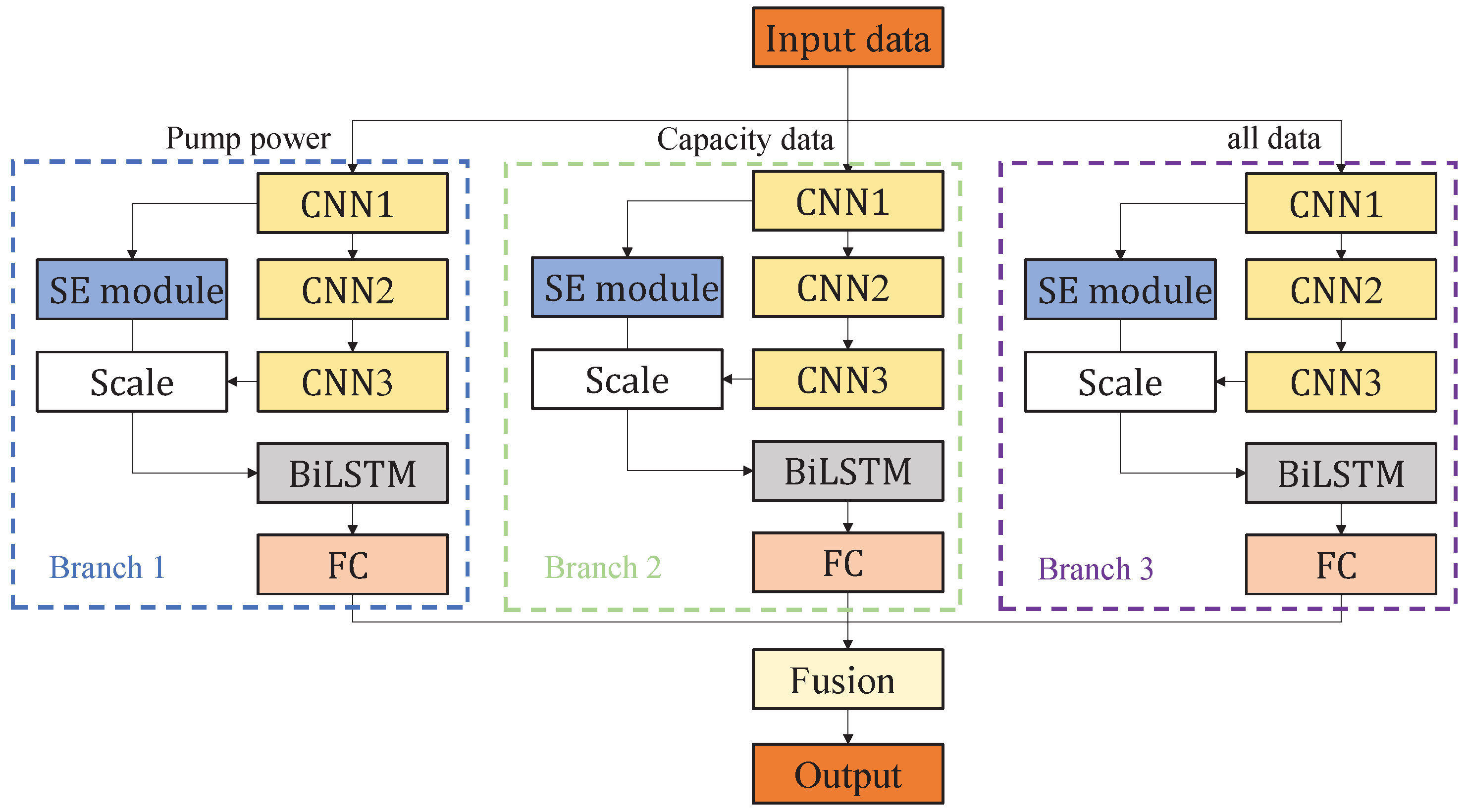
In this paper, a Multi-Branch Attention–CNN–BiLSTM network is designed for upper and lower reservoir capacity forecasting. The model takes BiLSTM as the baseline forecast model and introduces the CNN to improve the feature extraction ability of the model on the time series, which helps the model to better handle the depth information of the time series. To further improve the model’s ability to pay attention to data processing, the CNN is tuned by using the SE attention mechanism. The data used in this paper include reservoir capacities, water levels, and pumping machine power, and different data have different correlations for reservoir capacities.

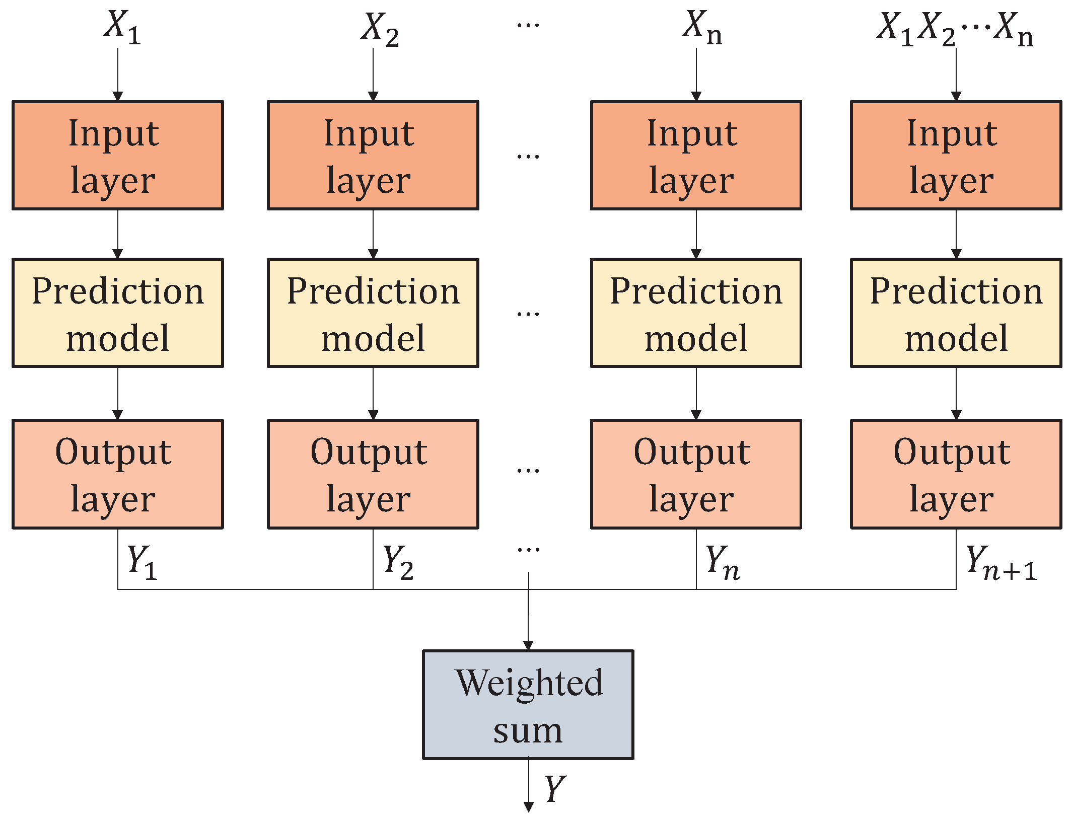
In order to better extract the relationship between different data and reservoir capacity, this paper adopted a multi-branch network model, and each branch adopts the same Attention–CNN–BiLSTM structure. The branches were fed with different data types, respectively, and one of the branches included all data types. Each branch obtained the forecast values of the reservoir capacities, and finally all the forecast values were fused together by the weighted sum to obtain the final forecast results. The structural framework of the Mulit-Branch Attention–CNN–BiLSTM forecast model is shown in Figure 3.

A three-branch structure was designed with one input for pump power, one input for reservoir capacity and level, and one input for all data. The weighted sum of the fusion modules uses the following formula:

$$Y=a_1\ast Y_1+a_2\ast Y_2+a_3\ast Y_3$$

(3)

where $Y_1$, $Y_2$, and $Y_3$ are the forecast outputs of the first, second, and third branches, respectively; $a_1$, $a_2$, and $a_3$ are the weights of the first, second, and third branches, respectively; and $a_1+a_2+a_3=1$. The corresponding weights were calculated based on the correlation coefficients in Table 2. The specific steps were calculating the average of the correlation coefficients of each channel and then calculating the weights based on the proportion of the three average correlation coefficients. The expression for weight calculation is

$$a_i={\displaystyle \frac{s_i}{s_1+s_2+s_3}}$$

(4)

where $a_i$ is the weight of the ith channel; $s_i$ is the average correlation coefficient of the ith channel; and $s_1,s_2,s_3$ are the average correlation coefficients of the three channels. In this paper, we used Spearman’s characteristic coefficient analysis and finally set $a_1=0.2444$; $a_2=0.3969$; and $a_3=0.3587$.

3.1. Bidirectional Long- and Short-Term Memory Network

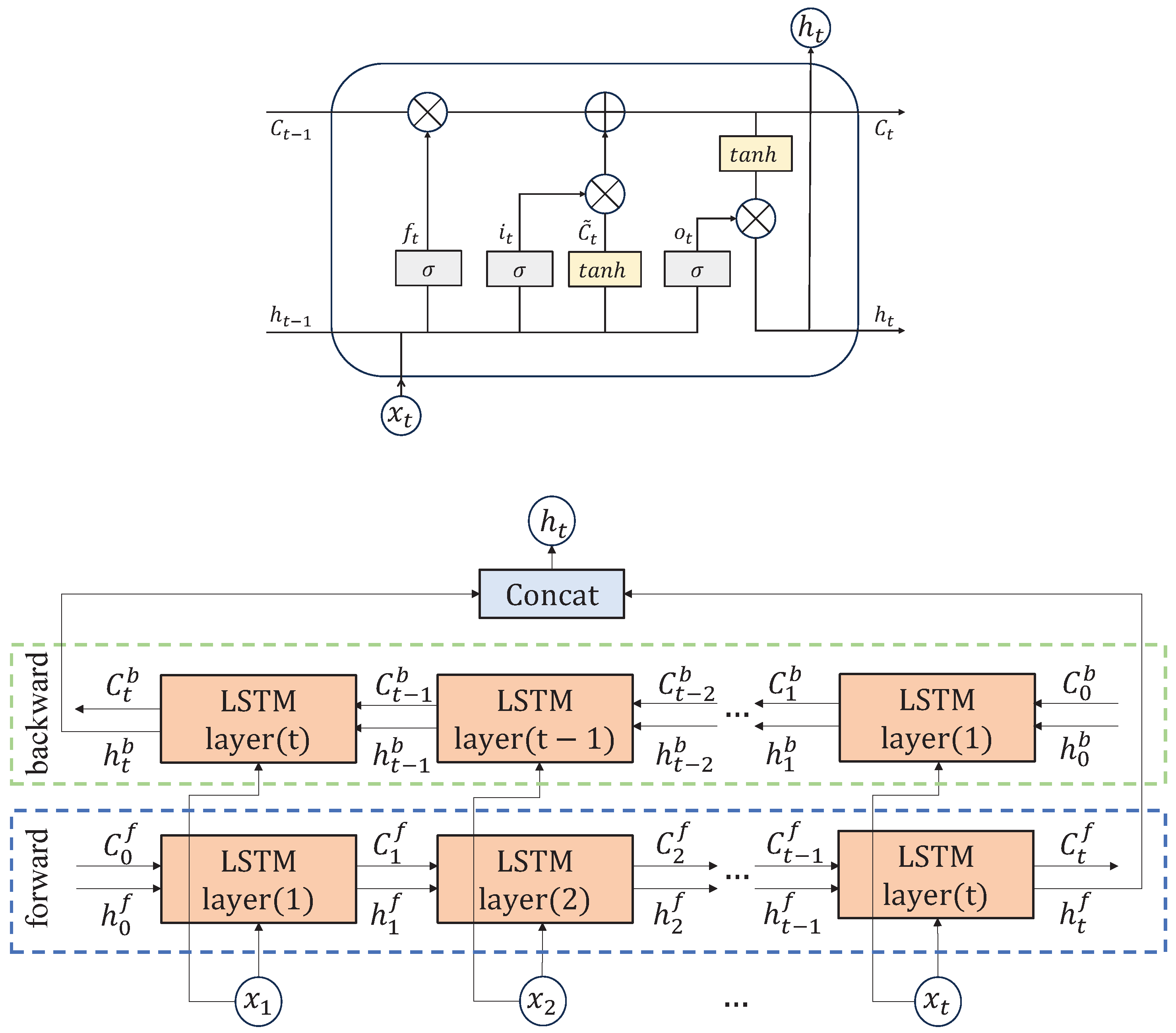
LSTM is a special RNN designed to solve the long-term dependency problem in sequence data. Although traditional RNNs are capable of handling sequence data, they perform poorly when dealing with long sequences due to the gradient vanishing or explosion problem. LSTM is able to alleviate this problem by introducing a gating mechanism which can effectively selectively remember or forget information. In addition, LSTM adds the cell state number C as a memory unit to correlate information over a longer time span. The core of LSTM consists of the forget gate, input gate, output gate, and cell state. The structural framework of the LSTM layer is shown in Figure 4.

(1)

Forget gate: The forget gate is used to control which historical information needs to be forgotten. A weight between 0 and 1 is generated for adjusting the forgetting ratio by weighting and summing the hidden state of the previous time step $h_{t-1}$ and the current input $x_t$ as well as activating it. The expression for the equation of the forget gate is given:

$$f_t=\sigma \left(W_f·\left[h_{t-1},x_t\right]+b_f\right)$$

(5)

where $W_f$ is the weight; $b_f$ is the bias; and $\sigma$ is the Sigmoid function. The expression for the equation of the Sigmoid function is given as follows:

$$f\left(x\right)={\displaystyle \frac{1}{1+e^x}}$$

(6)

(2)

Input gate: The input gate determines which parts of the information from the current time step need to be added to the cell state and regulates the strength of the information update by an activation function that combines the current input and the previous hidden state. The expressions for the equations of the input gate are given as follows:

$$i_t=\sigma \left(W_i·\left[h_{t-1},x_t\right]+b_i\right)$$

(7)

$${\tilde{C}}_t=tanh\left(W_C·\left[h_{t-1},x_t\right]+b_C\right)$$

(8)

where $W_i$ and $W_C$ are weights; $b_f$ and $b_C$ are biases; and tanh is the Tanh function. The expression for the equation of the Tanh function is

$$f\left(x\right)={\displaystyle \frac{e^x-e^{-x}}{e^x+e^{-x}}}$$

(9)

(3)

Output gate: The output layer is used to regulate and output the hidden state output from the LSTM in the current time step, which contains extensive time-dependent information and is adapted to the current time step. The expression for the equations of the output gate are

$$o_t=\sigma \left(W_o·\left[h_{t-1},x_t\right]+b_o\right)$$

(10)

$$h_t=o_t·tanh\left(C_t\right)$$

(11)

where $W_o$ is the weight; $b_o$ is the bias; and $C_t$ is the current cell state number.

(4)

Cell state: The cell state is an important carrier of LSTM memory, which keeps the long-term memory of sequence data by discarding part of the old information through the forget gate and then introducing new information in combination with the input gate. The expression for the equation of the cell state is

$$C_t=f_t·C_{t-1}+i_t·{\tilde{C}}_t$$

(12)

The structure of LSTM can only process sequence data from front to back sequentially, which may ignore the effect of future time steps on current time steps. In many practical applications, however, future information often plays an important role in current judgment as well. For this reason, scholars have researched BiLSTM. BiLSTM processes sequence data from two directions by using two independent LSTM layers in both forward and backward directions. Forward LSTM extracts forward-dependent features of the time step from the sequence start point to the end point; backward LSTM extracts backward-dependent features of the time step from the sequence end point to the start point. The features in these two directions are eventually weighted and merged to generate a complete contextual representation of each time step, thus improving the model’s ability to understand the sequence data. The structural framework of BiLSTM is shown in Figure 4. Both forward and backward LSTMs learn the input data to obtain their respective hidden states with long-term dependence. BiLSTM connects the two hidden states, allowing the model to understand the time-series data in a more comprehensive way, which is suitable for complex forecast tasks.

3.2. Convolutional Neural Network and SE Attention Mechanism Design

In the regression forecast for reservoir capacities, the CNN can efficiently extract local patterns in time series data and reduce noise interference and provide high-quality feature representations for the subsequent forecast process. The CNN is mainly responsible for extracting local patterns and key features in the input data in CNN-BiLSTM-based regression forecasting, which provides more effective feature representation for subsequent time-dependent modeling. The CNN extracts local feature patterns from the input data through convolutional layers, such as short-term trends and key changes in the time series, and significantly reduces the computational complexity of the network by utilizing parameter sharing and local connectivity. The superposition of multiple convolutional layers enables the model to progressively extract more abstract features from low to high levels. In order to capture nonlinear relationships, the output after convolution is usually nonlinearly mapped by an activation function (e.g., ReLU), which provides the model with stronger expressive capability. To better extract the feature relationship between the data, this paper uses the connection of three convolutional layers, and the convolutional layers are connected by the ReLU activation function.

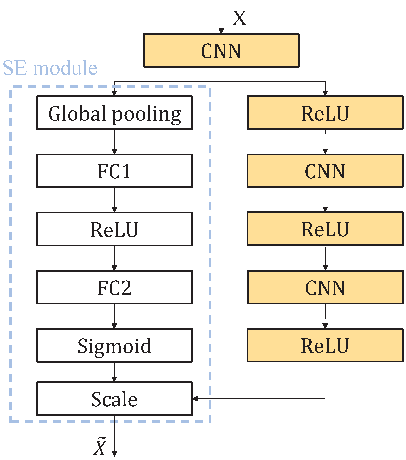
In traditional neural networks, the model processes the input data uniformly and does not differentiate between the attention paid to different parts. However, when processing longer time series, some parts may be more important than others. The purpose of the attention mechanism is to enable the model to selectively focus on the interested or critical parts of the data sequence, enabling further improvements in model accuracy. In this paper, we use the SE attention mechanism to improve the CNN network to help the model accurately capture key features and effectively reduce the interference of irrelevant information in the model. The SE attention mechanism is a lightweight but efficient channel attention mechanism that focuses on improving the feature representation of the CNN. Traditional CNNs assign the same importance to all channels by default when processing features, but in real tasks the contribution of different channels to the final goal often has differences.The SE attention mechanism improves the performance of the model by dynamically adjusting the weights of each channel to emphasize the important feature channels, while suppressing irrelevant or redundant channel information. The SE module consists of three parts: global information embedding (Squeeze), adaptive recalibration (Excitation), and reweighting (Scale). The structure of SE attention in the CNN is shown in Figure 5.

In the SE attention mechanism, the number of channels in the previous fully connected layer (FC) is 1/8 of the number of channels in the latter FC; the number of channels in the latter FC is equal to the number of channels in the last CNN layer. In the Squeeze stage, the SE module compresses the spatial information of each channel through global average pooling, generates the global feature description and extracts the key channel correlations; in the Excitation stage, the dependencies between channels are learned through a series of fully connected layers and activation functions, and the weighting coefficients are generated. In the Scale stage, the weights obtained earlier are reused on the original feature map to realize the dynamic adjustment of the channel features, thus improving the expressive ability of the model.

3.3. Multi-Branch Network for Attention–CNN–BiLSTM

To fully exploit the role of multi-source information in the forecast task, the multi-branch network structure has been widely adopted in SE Attention–CNN–BiLSTM forecast networks. By building a branch network to receive different categories of factors related to the target variable separately, a comprehensive input branch is introduced at the same time which is used to capture the global pattern of the overall features. The branch network structure is shown in Figure 6.

The structure of each branch of a multi-branch network is kept consistent by extracting feature representations of different inputs and fusing them in subsequent layers. Weighted fusion, an attention mechanism, or feature splicing are usually adopted in the fusion stage to ensure that the importance of different sources of information in decision making is reasonably expressed. Compared with the traditional single structure, models based on multi-branch design can more effectively separate and utilize relevant information from multi-source data, while demonstrating significant performance advantages in scenarios with complex data features or diverse sources. This structure provides a general and efficient solution for reservoir capacity forecasting.

4. Experiment Results

In this paper, Multi-Branch Attention–CNN–BiLSTM was used to predict the capacity of the upper and lower reservoirs. The input data included the power of U01, the power of U03, and the water level and capacity of the upper and lower reservoirs in the last five steps, each with a time interval of 30 min. The output data were the upper and lower reservoir capacities in the next step. The dimension of input data was 40 and the dimension of output data was 2. The training data were converted to 6473 rows and the test data were 341 rows according to the model data requirements. Multi-Branch Attention–CNN–BiLSTM was trained using the training data and the model was tested by using the test data. The model was validated by using metrics such as the $MAPE$, the $RMSE$, and $R^2$, as well as scatter plots and distribution plots, to ensure correct forecasting of the model.

4.1. Model Training

In order to conduct the model training, this paper set appropriate Multi-Branch Attention–CNN–BiLSTM model parameters. The Multi-Branch Attention–CNN–BiLSTM model parameters are shown in

Table 3. Multi-Branch Attention–CNN–BiLSTM model parameters.

Parameter	Value
Number of CNN1 channels	64
Number of CNN2 channels	32
Number of CNN3 channels	32
Number of FC1 channels for SE	4
Number of FC2 channels for SE	32
Neuron count of BiLSTM hidden layer	32
Weighted argument	[0.2444, 0.3969, 0.3587]

. To balance the capability of the model and the computational complexity, 32 BiLSTM hidden-layer neurons were set in this paper. The number of channels of the CNN layer was set to 64 channel counts for the first layer and 32 for both the second and the third layers, which helped the model to extract multi-layered features from the original data and reduced the computational complexity and the risk of overfitting. To ensure the reliability of the weighted sums of the different branches, this paper scaled the division based on the correlation between the input data and the output data. The correlations of the input data of the three branches were averaged and the three averages were converted to a value whose sum was equal to one. The final weighted ratios were $a_1=0.2444$; $a_2=0.3969$; and $a_3=0.3587$.

4.2. Model Testing

In this paper, the $MAPE$, the $RMSE$, and $R^2$ were used to statistically forecast the accuracy of the model. The $MAPE$ is the mean absolute percentage error, which does not change due to global scaling of the variables. $RMSE$ is the root mean square error, which measures the deviation of forecast values from actual observations. $R^2$ is the coefficient of determination, which is a visual representation of the accuracy of the model and can take values between 0 and 1. The smaller the values of the $MAPE$ and $RMSE$ are, the higher the forecast accuracy of the model is; the closer $R^2$ is to 1, the higher the forecast accuracy of the model is; and the closer $R^2$ is to 0, the worse the forecast accuracy is. The expressions of the $MAPE$, the $RMSE$, and $R^2$ are

$$MAPE={\displaystyle \frac{100\%}{n}}\sum _{i=1}^n\left|{\displaystyle \frac{{\widehat{y}}_i-y_i}{y_i}}\right|$$

(13)

$$RMSE=\sqrt{{\displaystyle \frac{1}{n}}\sum _{i=1}^n{\left({\widehat{y}}_i-y_i\right)}^2}$$

(14)

$$R^2=1-{\displaystyle \frac{{\displaystyle \sum _{i=1}^n}{\left({\widehat{y}}_i-y_i\right)}^2}{{\displaystyle \sum _{i=1}^n}{\left({\overline{y}}_i-y_i\right)}^2}}$$

(15)

where ${\widehat{y}}_i$ is the forecast value; $y_i$ is the actual value; ${\overline{y}}_i$ is the average value; and n is the size of the data.

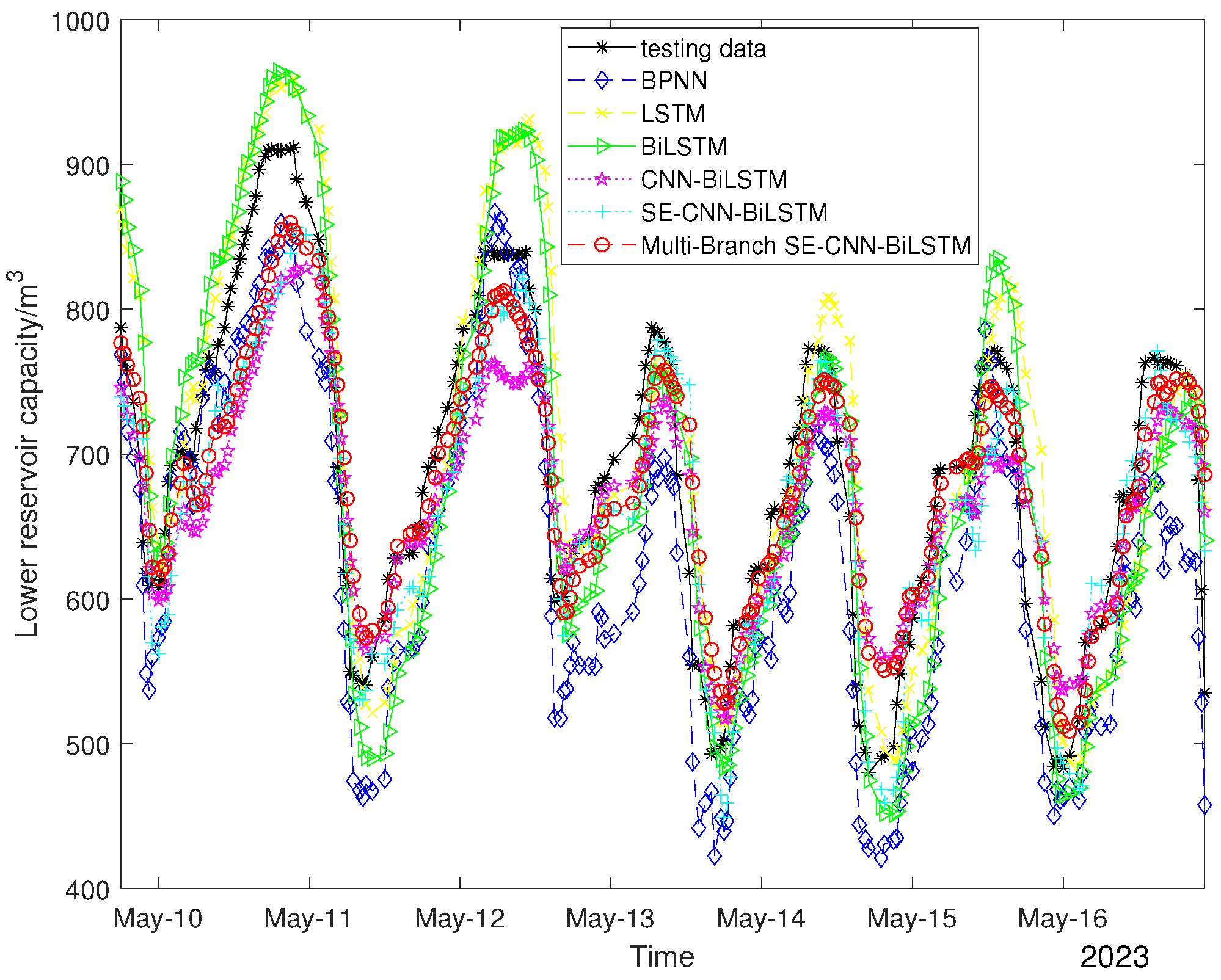
To verify the effectiveness of Multi-Branch Attention–CNN–BiLSTM in this work, multiple models were used for comparison including the original LSTM model, the original BiLSTM model, CNN-improved BiLSTM (CNN-BiLSTM), and SE attention mechanism-improved CNN-BiLSTM (SE-CNN-BiLSTM). In addition, in order to verify that the LSTM family of models has a better forecast ability for time series data, the BPNN model was introduced for comparison. The forecasts of the upper reservoir, lower reservoir, and average capacities in different models are respectively shown in the

Table 4. Forecast of upper reservoir capacity in different models.

Model	${\mathit{R}}^2$	$\mathit{MAPE}$/%	$\mathit{RMSE}$$/{\mathbf{m}}^3$
BPNN	0.7492	5.1171	48.5605
LSTM	0.7876	4.8442	44.6952
BiLSTM	0.7953	4.8153	43.8756
CNN-BiLSTM	0.8533	3.8837	33.9849
SE-CNN-BiLSTM	0.9114	2.8628	28.8582
Multi-Branch Attention–CNN–BiLSTM (ours)	0.9231	2.8853	26.8869

,

Table 5. Forecast of lower reservoir capacity in different models.

Model	${\mathit{R}}^2$	$\mathit{MAPE}$/%	$\mathit{RMSE}$$/{\mathbf{m}}^3$
BPNN	0.6077	9.0973	68.0587
LSTM	0.6480	7.7414	64.4664
BiLSTM	0.6966	7.6735	59.8526
CNN-BiLSTM	0.7278	6.8283	51.8828
SE-CNN-BiLSTM	0.7949	5.8887	49.2135
Multi-Branch Attention–CNN–BiLSTM (ours)	0.8242	5.4251	45.5623

, and

Table 6. Average forecast of upper and lower reservoir capacities in different models.

Model	${\mathit{R}}^2$	$\mathit{MAPE}$/%	$\mathit{RMSE}$$/{\mathbf{m}}^3$	Time/s
BPNN	0.6785	7.1072	58.3096	0.0190
LSTM	0.7178	6.2928	54.5808	0.0084
BiLSTM	0.7460	6.2444	51.8641	0.0098
CNN-BiLSTM	0.7906	5.3560	42.9339	0.0211
SE-CNN-BiLSTM	0.8531	4.3758	39.0359	0.0217
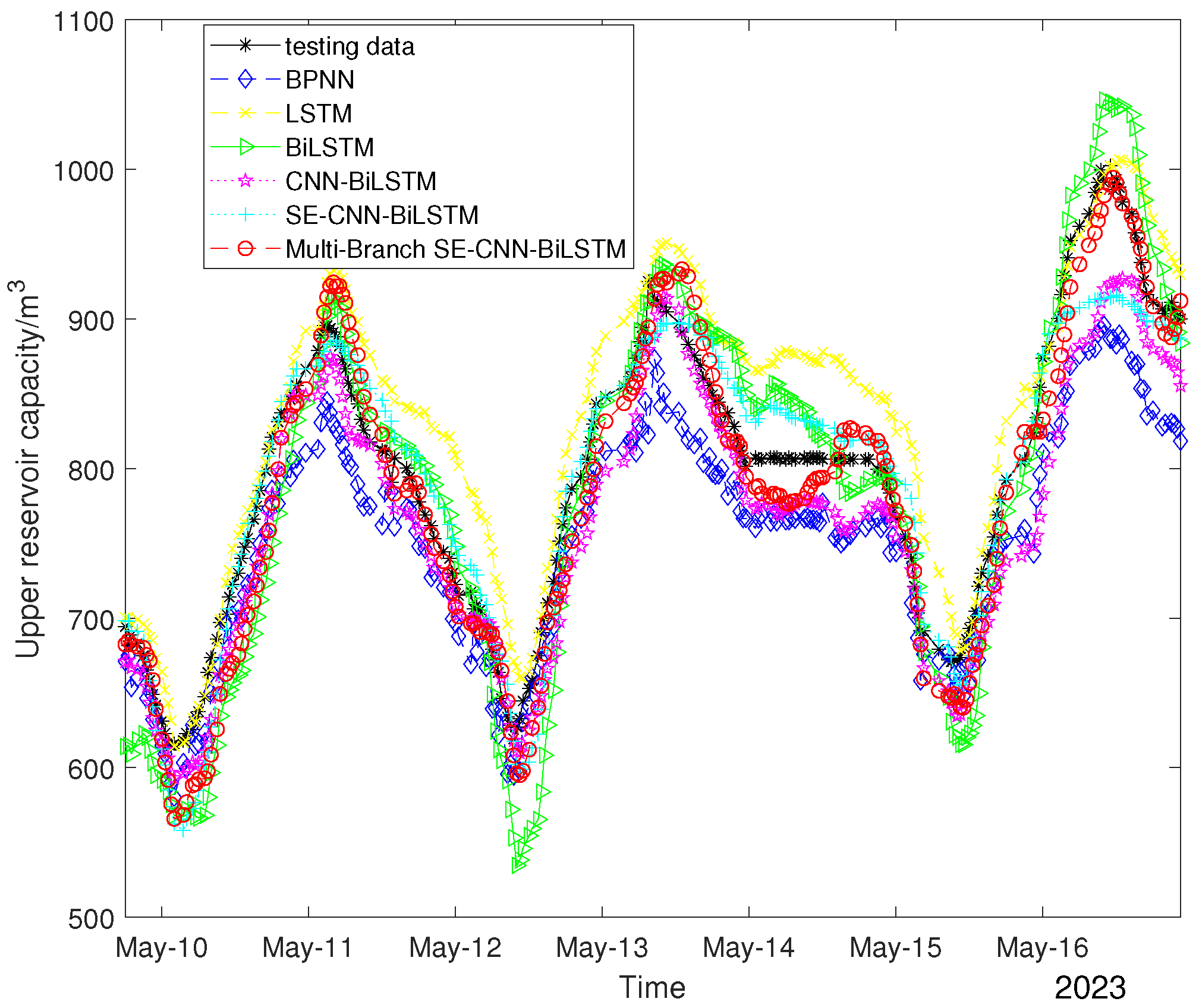
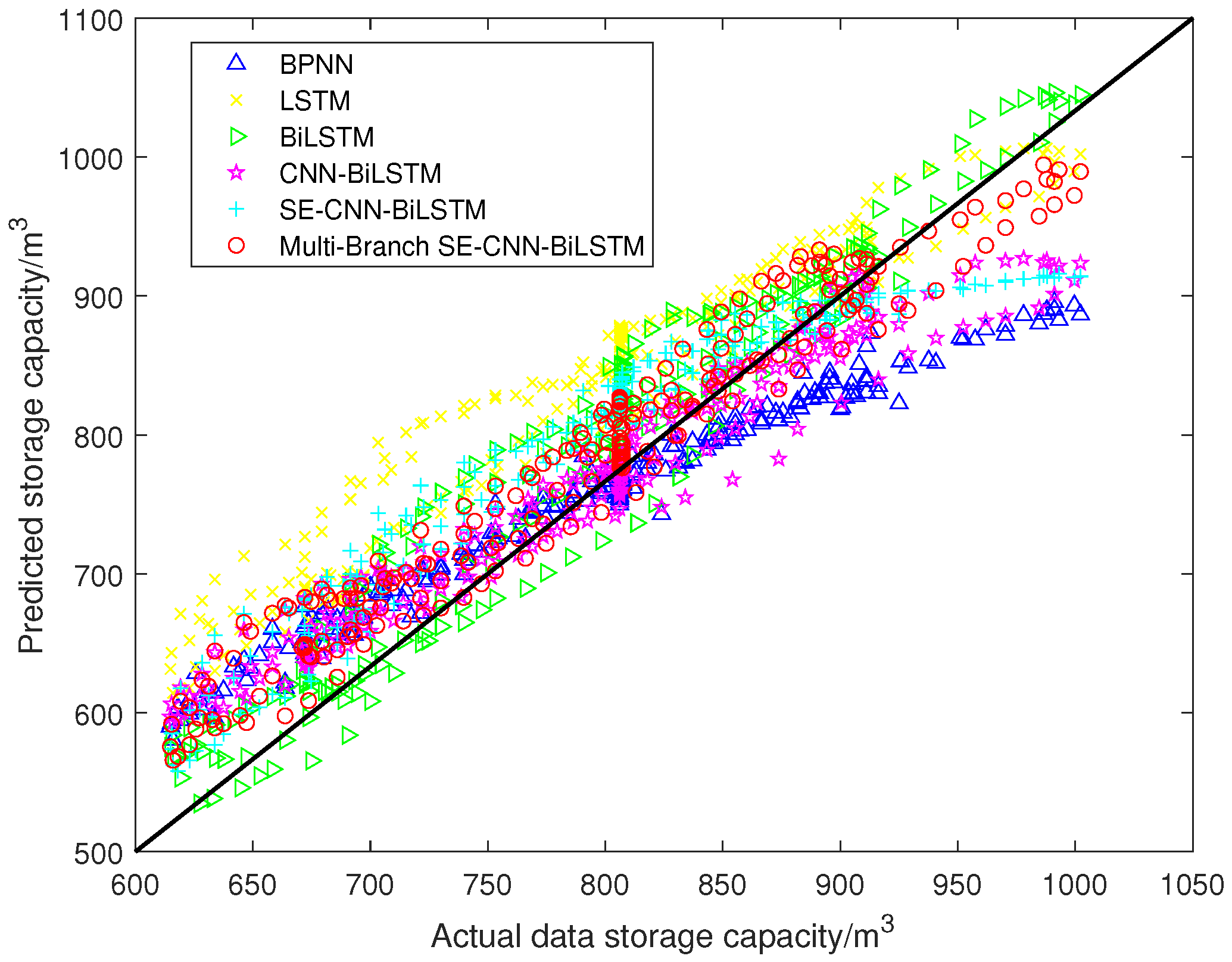
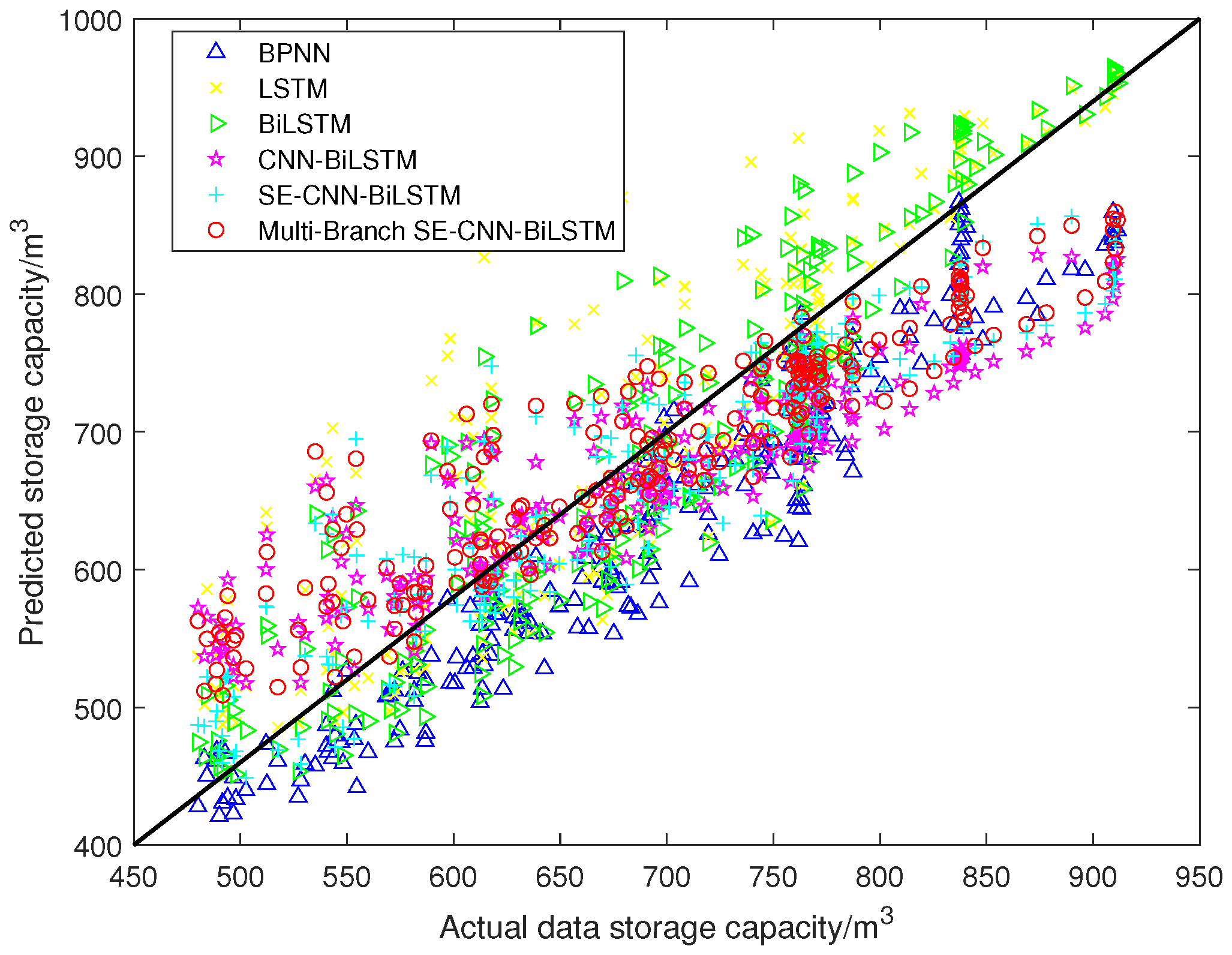
Multi-Branch Attention–CNN–BiLSTM (ours)	0.8737	4.1552	36.2246	0.0525

. The distribution and scatter plots of the forecast values of different models on the test data are plotted. The distribution and scatter plots of the upper reservoir capacity forecast results are shown in Figure 7 and Figure 8. The distribution and scatter plots of the lower reservoir capacity forecast results are shown in Figure 9 and Figure 10.

As can be seen from Figure 7, Figure 8, Figure 9 and Figure 10, the Multi-Branch SE–CNN–BiLSTM designed in this paper had the best results in the double-output forecast of the upper and lower reservoirs, and our model could complete the forecast of the upper and lower reservoir capacities. This is not only reflected in its ability to follow the trend of the actual data but also in the alignment of the predicted values with the actual values in the scatter distribution plots. In Figure 7 and Figure 9, the predicted curves of the Multi-Branch SE–CNN–BiLSTM model are closest to the actual data curves, indicating that the model was able to effectively capture the dynamic changes in the data. In Figure 8 and Figure 10, the point-to-point distributions of predicted and actual values are closest to the diagonal line, which further validates the high accuracy of the Multi-Branch SE–CNN–BiLSTM model model predictions. Both LSTM and BiLSTM achieved better forecast results compared to the BPNN, which indicates that the BPNN is not ideal for performing time series processing. From the tab4,tab5,tab6, it can be seen that Multi-Branch SE–CNN–BiLSTM predicted the upper reservoir capacity with an $R^2$ of 0.9231, $MAPE$ of 2.8853%, and $RMSE$ of 26.8869 ${\mathrm{m}}^3$; and it predicted the lower reservoir capacity with an $R^2$ of 0.8242, $MAPE$ of 5.4251%, and $RMSE$ of 45.5623 ${\mathrm{m}}^3$. The average metrics for the two reservoir capacities were an $R^2$ of 0.8737, $MAPE$ of 4.1552%, and $RMSE$ of 36.2246 ${\mathrm{m}}^3$. The computing time of Multi-Branch Attention–CNN–BiLSTM was only 0.0525 s, which is very short time for the considered problem, although it required more computing time compared to other models. This is due to the fact that Multi-Branch Attention–CNN–BiLSTM has a more complex model architecture.

The introduction of the CNN and SE attention mechanisms substantially improves the forecast accuracy of the model. The upper and lower reservoir capacity $MAPE$ of CNN-BiLSTM was improved by 0.9316% and 0.8452% compared to that of BiLSTM, respectively, and the mean of the two was improved by 0.8884%; the upper and lower reservoir capacity $MAPE$ of SE-CNN-BiLSTM was improved by 1.0209% and 0.9396% compared to that of CNN-BiLSTM, and the mean of both was improved by 0.9802%. The introduction of the multi-branch model improved the forecast accuracy of the lower reservoir capacity and further ensured the accuracy of the double-output model forecast. The introduction of the multi-branch model made the model forecast values more closely match the distribution of the actual data, which indicates the reliability of multi-branch improvement in the double-output forecast of the upper and lower reservoirs.

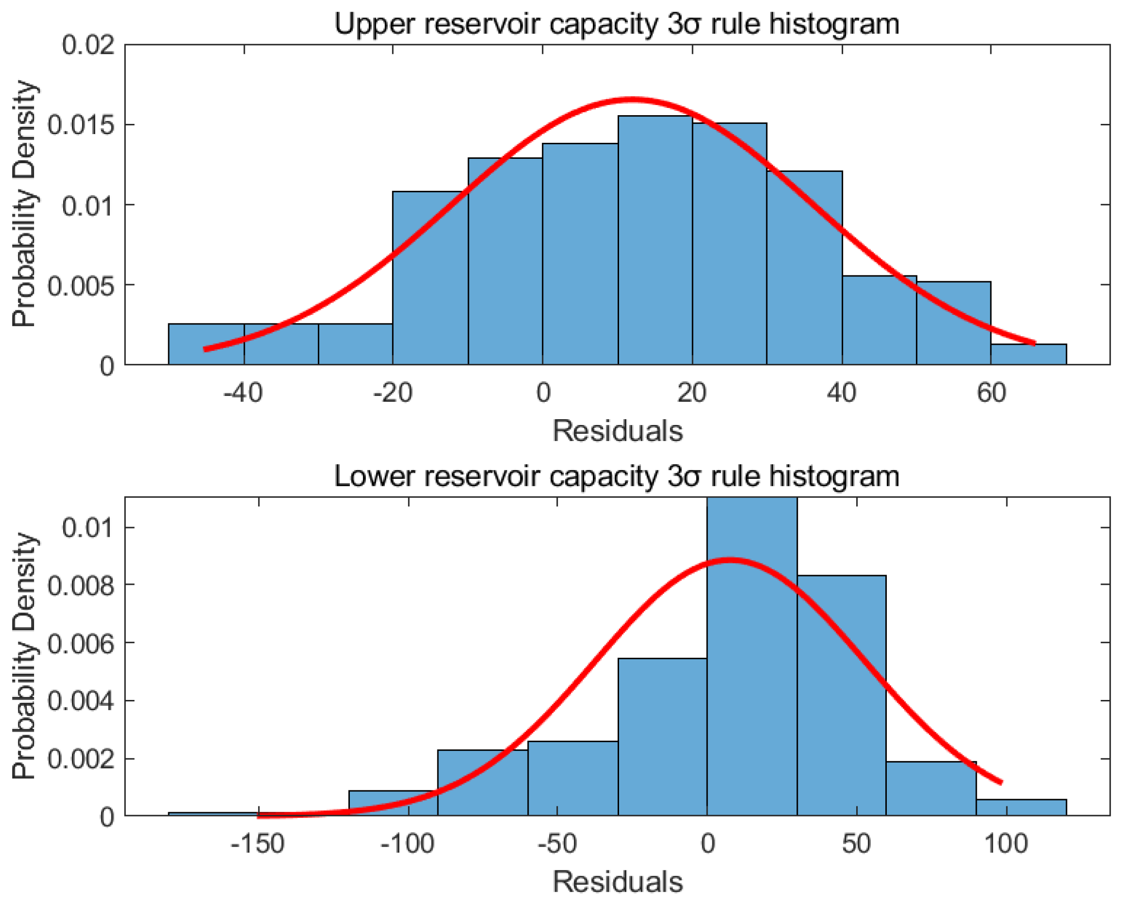
The 3$\sigma$ rule is used to assess the reliability of the forecast of a predictive model. In statistics, data are normally distributed in principle, and the percentage of values that are less than one standard deviation, two standard deviations, and within three standard deviations from the mean are the precise figures of 68.27%, 95.45%, and 99.73%. Therefore, it can be assumed that a data value is almost distributed within the interval $(\mu -3\sigma ,\mu +3\sigma )$, and the probability of exceeding this range is less than 0.3%. After the forecast model generates results, the mean and standard deviation of the distribution of forecast values can be calculated as a way of determining whether certain forecast values are outside a reasonable range. When the forecast result exceeds three times the standard deviation, it indicates that there is an error in the model or an anomaly in the forecast target data. By analyzing these anomalous results, it can be found to provide a warning for the forecast target to avoid loopholes or equipment problems in the daily production process.

In this paper, the difference between the actual and forecast data was calculated separately for the upper and lower reservoir capacities, and the 3$\sigma$ ReLu historgram of the difference was analyzed. The mean value of the upper reservoir capacity residual was 11.9863 ${\mathrm{m}}^3$ and the standard deviation was 24.1193 ${\mathrm{m}}^3$; the mean value of the lower reservoir capacity residual was 7.6263 ${\mathrm{m}}^3$ and the standard deviation was 45.0166 ${\mathrm{m}}^3$. The 3$\sigma$ ReLu historgram of the error of the upper and lower reservoir capacity is shown in Figure 11. Therefore, the error distribution of the upper reservoir capacity is $(-60.3716{\mathrm{m}}^3,$$84.3442{\mathrm{m}}^3)$, and the range of error distribution for the lower reservoir capacity is $(-127.4235{\mathrm{m}}^3, 142.6761{\mathrm{m}}^3)$. When the residuals exceed these ranges, there may be a problem with the upper and lower reservoir capacities, such as leakage. This information allows workers to provide real-time maintenance to ensure the safe operation of a pumped storage hydropower plant.

5. Conclusions

In this paper, the Multi-Branch Attention–CNN–BiLSTM forecast model was developed to predict the upper and lower reservoir capacities of pumped storage hydropower plants. The correlation of the data was analyzed using Spearman’s characteristic coefficients, and the power of $U01$, the power of $U03$, and the level and the capacity of the upper and lower reservoirs were selected to predict the capacity of the upper reservoir. The experimental results show that the Multi-Branch Attention–CNN–BiLSTM model exhibits higher accuracy in predicting the reservoir capacity of pumped storage hydropower plants compared to the baseline model. Compared with the original BiLSTM, the forecast results were closest to the trend of the test data, with an increase of $1.9300\%$ and $2.2484\%$ in the $MAPE$, $16.9887{\mathrm{m}}^3$ and $14.2903{\mathrm{m}}^3$ in the $RMSE$, and $0.1278$ and $0.1276$ in $R^2$, respectively. Using the Multi-Branch Attention–CNN–BiLSTM model, the average metrics for the two reservoir capacities were an $R^2$ of 0.8737, $MAPE$ of 4.1552%, and $RMSE$ of 36.2246 ${\mathrm{m}}^3$. The error distribution ranges of the upper and lower reservoir capacities were obtained based on 3$\sigma$ as $(-60.3716{\mathrm{m}}^3,84.3442{\mathrm{m}}^3)$ and $(-127.4235{\mathrm{m}}^3,142.6761{\mathrm{m}}^3)$, respectively, and such information can provide a real-time maintenance strategy to ensure the safe operation of pumped storage hydropower plants. The prediction model proposed in this paper has dual outputs, and the change in the lower reservoir capacity is more unstable than the change in the upper reservoir capacity, which leads to a larger error range in the lower reservoir capacity.