Monitoring and Suppression Strategies of the Interharmonic in the Grid-Connected Photovoltaic System: A Review

Abstract

With the continuous advancement of the green and low-carbon transformation of energy structures in countries around the world, renewable energy sources such as solar energy are receiving increasingly widespread attention. Driven by this trend, photovoltaic (PV) power generation, with its unique advantages, has continuously increased the scale of PV grid connection. However, the inherent characteristics of solar energy and the control features of grid-connected PV systems result in the presence of a large amount of interharmonic components in their output current, seriously endangering the safety and stable operation of the power system. Since interharmonics are difficult to obtain in an intuitive way, this paper first introduces the monitoring methods of interharmonics. Based on accurately monitoring the interharmonics, further discussions were carried out around the interharmonic suppression strategies. Through the analysis of the advantages and disadvantages of various interharmonic monitoring methods and suppression strategies, guidance can be provided for the selection of interharmonic monitoring methods and suppression strategies in different scenarios.

1. Introduction

In recent years, countries around the world have been actively promoting the green and low-carbon transformation of energy. Renewable energy sources such as solar energy, wind energy and ocean energy, with their environmentally friendly and sustainable characteristics, have become key areas in the energy transition of various countries. Among numerous renewable energy sources, solar energy has been favored by various countries due to its advantages such as being clean, pollution-free and having abundant reserves. Solar energy is playing an increasingly important role in the energy transition [1]. The grid connection of photovoltaic (PV) power generation can not only reduce carbon emissions, optimize the energy structure and bring significant environmental benefits, but it can also drive industries, stabilize energy prices and create economic benefits. Therefore, under the wave of energy transition, the large-scale grid connection of PV power generation will become an inevitable trend. However, due to the inherent characteristics of solar energy and the control features of grid-connected PV systems, PV output shows strong randomness and volatility. 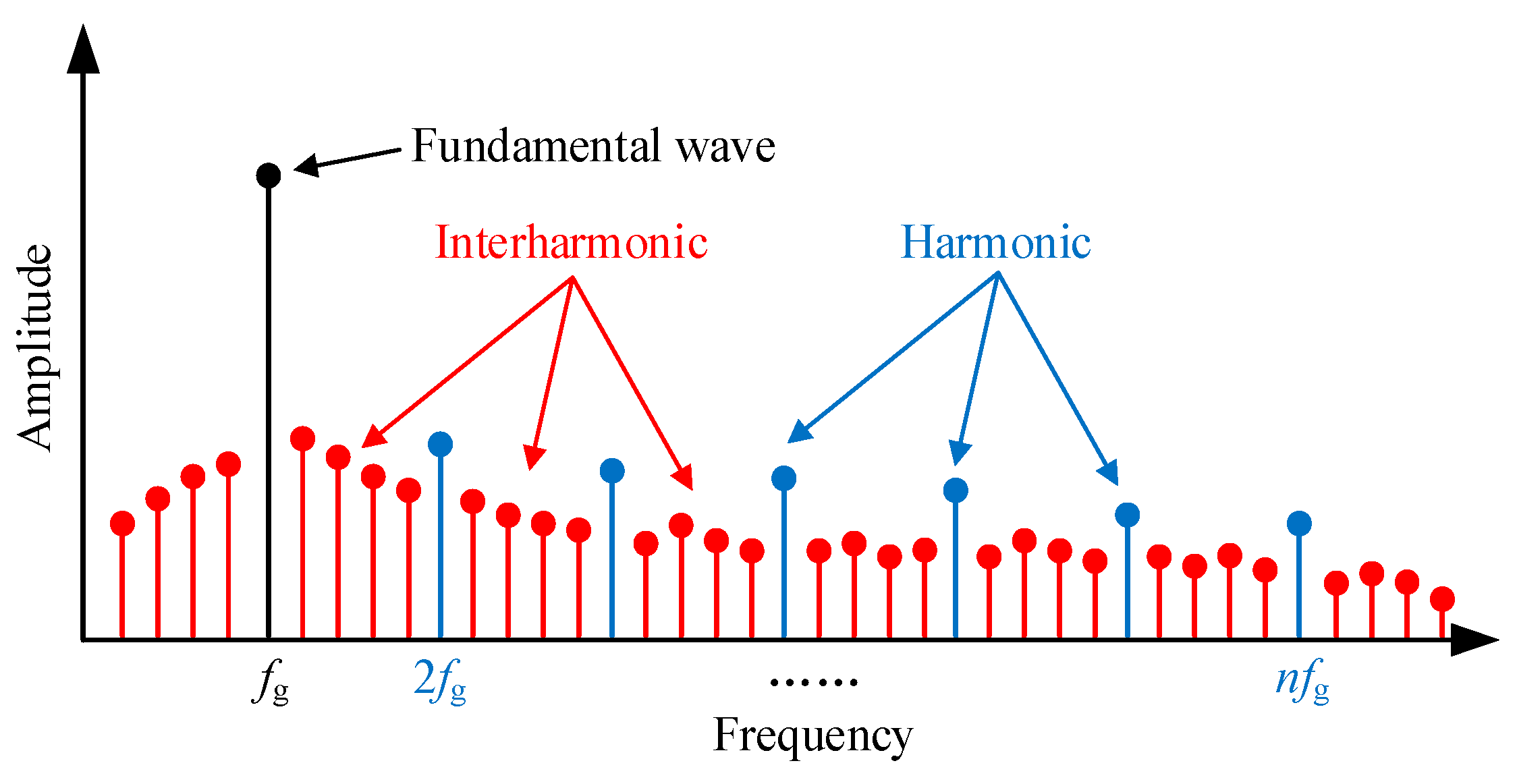Furthermore, the large-scale investment in nonlinear power electronic devices and the application of the maximum power point tracking (MPPT) algorithm will bring complex harmonic and interharmonic problems to the power grid [2,3], seriously reducing the power quality of the power system. Among them, the interharmonic refers to the component whose frequency is a non-integer multiple of the fundamental frequency. The distribution of harmonic current and interharmonic current in the grid-connected PV system [4] is shown in Figure 1.

Mao et al. [5] conducted a comprehensive analysis of the influencing factors of interharmonics in PV grid-connected systems. For the single-stage PV grid-connected system, the perturbation-based MPPT algorithm was adopted. The inverter controller adopted a voltage-current dual closed-loop structure based on PI control. The simulation test of the PV grid-connected system was conducted according to the parameters set in

Table 1. Main parameters of the PV grid-connected system.

Parameters	Values	Parameters	Values
Open circuit voltage	876 V	Grid phase voltage	220 V
Short circuit current	8.31 A	Grid frequency	50 Hz
Maximum power point voltage	700 V	Direct current capacitor	1000 µF
Maximum power point current	7.58 A	Filter inductance	6 mH
Maximum power output	5.3 KW	Switching frequency	10 kHz
Illumination intensity	1000 W/m2	Battery temperature	25 °C
Disturbance period	0.05 s	Disturbance step size	5 V

. The current spectrum of phase A is shown in Figure 2.

At present, many scholars have conducted research on the generation mechanism of interharmonics in grid-connected PV systems. Pakonen et al. [6] proved with detailed experimental data that the MPPT algorithm is the main cause of interharmonic current generation in grid-connected PV systems. Moreover, the interharmonic frequency generated by this algorithm is extremely close to the frequency at which the human eye is most sensitive to changes in light brightness. In [7], through rigorous experimental analysis, it was also verified that the MPPT algorithm is the main cause of the generation of interharmonic currents. Meanwhile, it was further found that the interharmonic currents generated by the MPPT algorithm are mainly distributed within the frequency range of 0–100 Hz, while the interharmonics with frequencies higher than 100 Hz can be ignored due to their extremely low content. While analyzing whether the MPPT algorithm is the main source of interharmonics in grid-connected PV systems, Langella et al. [8] pointed out that the relative level of interharmonic current in grid-connected PV systems is greatly affected by the actual power. Sangwongwanich et al. [9] expound on the detailed process of interharmonics generated in grid-connected PV systems caused by the MPPT algorithm, as follows: At the beginning of each MPPT cycle, the sudden change of the direct current (DC) voltage command output by the MPPT will cause the voltage loop to rapidly generate a voltage error determined by the MPPT perturbation step. This error will pass to the current loop through the controller and eventually generate an interharmonic current under modulation.

After understanding the generation mechanism of interharmonics in grid-connected PV systems, the negative impacts brought by interharmonics need to be given more attention. Compared with harmonics, interharmonics have a wider distribution range, are more difficult to analyze and can cause more serious harm to power systems and related equipment. In terms of the stability of the power system, when the interharmonic frequency is in the sub-synchronous frequency band, it will interact with the mechanical oscillation of the adjacent generator shafting. This further induces sub-synchronous oscillations of the system [10,11,12,13]. Some scholars once investigated a damaging accident of a steam turbine generator in the United States. The investigation results indicated that the interharmonic component with a frequency of 55 Hz in the system current affected the amplitude modulation of the 60 Hz fundamental wave, thereby leading to the occurrence of the accident [14]. Moreover, the waveform distortion caused by interharmonics can have a negative impact on the normal operation of relay protection equipment and may even lead to its malfunction. Wang et al. [15] conducted research on the impact of interharmonics on relay protection devices and found that interharmonics would interfere with the normal operation of harmonic detection equipment and weaken the safety and stability of relay protection devices. The low-frequency interharmonic with a relatively high amplitude can also cause the visual response of the human eye to incandescent lamps, resulting in flickering [16,17,18]. In addition, interharmonics can also reduce the power factor of the system, resulting in a decline in the quality of grid-connected power. It will have an adverse impact on the operational efficiency and reliability of the entire power system.

In [19], the interharmonic monitoring methods for stationary time-varying signals are reviewed and compared. Ravindran et al. [20] further expand the scope of the review and analyze the challenges faced by each method. The above-mentioned reviews have only conducted a comprehensive analysis of the monitoring methods for interharmonics. This paper extends the monitoring method of interharmonics to the suppression strategy. While introducing the methods for monitoring interharmonics, the existing interharmonic suppression strategies are classified and discussed. This can provide certain ideas for future research on interharmonic suppression strategies.

The research motivation and contributions of this paper can be summarized as follows:

• The paper successively describes what interharmonics are, the generation mechanism of interharmonics and their hazards. To reduce the harm caused by interharmonics, the monitoring methods and suppression strategies of interharmonics were discussed successively.
• According to the characteristics of each method, the monitoring methods of interhar-monics are classified into four categories for introduction, and the advantages and disadvantages of each method are analyzed. The corresponding method can be selected according to the actual needs.
• The suppression strategies of interharmonics were sorted out based on three aspects. The strategies were also introduced and their advantages and disadvantages were analyzed. Based on the content of this paper, the prospects for future research on suppression strategies were proposed.

The rest of the paper is organized as follows. Section 2 introduces the monitoring methods of interharmonics. Section 3 describes different types of interharmonic suppression strategies. Section 4 has a discussion. Section 5 gives the conclusion.

2. Monitoring Methods for Interharmonics

The accurate monitoring of interharmonics is the primary link to suppress the hazards of interharmonics. It has always been a research hotspot in both the academic and industrial fields [21]. Due to the complexity and diversity of the power system, experts and scholars have proposed various interharmonic monitoring methods. Each of these methods has its advantages and is applicable in different scenarios. Based on the differences in monitoring principles and technical paths, this section mainly classifies the interharmonic monitoring methods into four categories. Figure 3 shows each monitoring method under different classifications.

In interharmonic monitoring, the sine model is often adopted to describe interharmonic disturbances [19]. This model characterizes the interharmonic signal as the superposition of multiple sine waves with different frequencies, amplitudes and phases. At the nth sample with sampling interval ∆t, the measured signal x(n) can be expressed as follows:

$$x(n)={\displaystyle \sum _{k=1}^K{a}_k\cos ({\omega }_{k}n\Delta t+{\varphi }_k)+w(n)}$$

(1)

where K represents the number of frequency components in the signal; $a_k$ represents amplitude; ${\varphi }_k$ represents the starting phase angle; the interharmonic frequency in radius ${\omega }_k=2\pi f_k$; $f_k$ is the kth frequency component; $w\left(n\right)$ is white Gaussian noise with zero mean.

The model in Equation (1) can also be expressed in the form of complex exponentials:

$$\left\{\begin{array}{c}x(n)={\displaystyle \sum _{k=1}^{2K}{A}_k{e}^{jn{\omega }_k\Delta t}+w(n)}\\ A_k={\displaystyle \frac{a_k}{2}}{e}^{j{\varphi }_k}\end{array}\right.$$

(2)

where $A_k$ represents complex amplitude.

2.1. Parametric Method

Parametric methods have become a research hotspot due to their high resolution and parameter interpretability. Parametric methods can directly estimate parameters such as frequency, amplitude and phase of harmonic components by constructing an explicit mathematical model of the signal. The core of this type of method lies in modeling the signal as a linear combination of several exponential or sinusoidal components, and solving the model parameters by using optimization or algebraic means. It can avoid the problem of energy dispersion caused by the non-integer period truncation of a finite-length signal (spectral leakage [22]) and significantly improve the analysis accuracy.

2.1.1. Estimation of Signal Parameters via Rotational Invariance Techniques (ESPRIT)

ESPRIT is a high-resolution parameterization method based on the decomposition of signal subspaces. The core idea is rotational invariance. By analyzing the rotational invariance of the signal subspace, the frequency parameters can be directly estimated without the need to search the entire spectrum. Based on Equation (2), its autocorrelation matrix can be constructed. And subspace decomposition is carried out on it to obtain the signal subspace $S_1$ and the noise subspace $S_2$, respectively [23].

Since there is rotational invariance between these two subspaces, it can be obtained from the following:

$$S_1=\Phi S_2$$

(3)

where the rotation factor matrix $\Phi =\left[\begin{array}{llll}{e}^{j2\pi f_1}\hfill & 0\hfill & \cdot \cdot \hfill & 0\hfill \\ 0\hfill & e^{j2\pi f_2}\hfill & \cdot \cdot \hfill & 0\hfill \\ \begin{array}{l}\cdot \\ \cdot \end{array}\hfill & \begin{array}{l}\cdot \\ \cdot \end{array}\hfill & \begin{array}{l}\cdot \\ \cdot \end{array}\hfill & \begin{array}{l}\cdot \\ \cdot \end{array}\hfill \\ 0\hfill & 0\hfill & \cdot \cdot \hfill & e^{j2\pi f_k}\hfill \end{array}\right]$ After obtaining the rotation factor matrix, the least square method can be used to solve the frequency-estimated value $f_k$ of the matrix Φ. According to the obtained frequency information, the amplitude and phase angle of the interharmonic components can finally be solved.

Aiming at the limitations of the traditional ESPRIT algorithm in the analysis of non-stationary signals, a sliding window ESPRIT method was proposed in [24]. This method achieves high-resolution estimation of the dynamic time-varying spectrum by dividing the signal into locally stationary sliding Windows and combining the pre-filtering technique to suppress the interference of the fundamental wave components. Jain et al. [25] proposed an improved ESPRIT method based on exact model order (EMO) estimation. This method innovatively introduces the relative difference index and the verification test mechanism. By analyzing the sudden change points of the eigenvalues of the autocorrelation matrix, a more exact division of the signal subspace and the noise subspace is achieved. In [26], an improved sliding window ESPRIT method was proposed. This method adopts a dynamic frequency tracking mechanism to calculate the frequency parameters only at the initial window or key nodes, and uses intelligent resampling technology to dynamically adjust the sampling rate. This resulted in the computational time of the improved ESPRIT being only 2.5% of that of the traditional ESPRIT, significantly enhancing the computational efficiency.

2.1.2. Prony’s Method

Prony’s method is a technique that approximates the sampled signal by using a finite set of indices of unknown frequencies, amplitudes and phase angles [27]. The key technique of Prony’s method is to introduce a polynomial $P\left(Z\right)$, whose exponential term contains frequency information as its root.

$$P(z)=\prod _{h=1}^M(z-z_h)$$

(4)

where polynomial $P\left(Z\right)$’s root $z_h=e^{j\omega }h\Delta t$; $M$ represents the estimated order.

To obtain these polynomial coefficients for identifying frequency components, various methods such as autocorrelation, covariance and singular value decomposition can be used. Finally, the amplitude and phase angle of each component can be tracked by constructing the Vandermonde matrix and solving its linear equation.

Chang et al. [28] proposed an improved Prony method. This method scales the signal in the frequency domain through downsampling technology and separates adjacent spectral lines into a distinguishable range. It significantly improves the frequency identification ability. Meanwhile, singular value decomposition (SVD) is adopted to solve the parameters of the Prony model, which enhances the robustness of the algorithm to noise. The reduced harmonic method proposed in [29] presets the interharmonic frequency vector and combines the undamped characteristics of the power grid signal. The polynomial rooting and SVD decomposition links in the traditional Prony method can be completely eliminated, and the deterministic Vandermonde matrix can be directly constructed for parameter estimation. Compared with the traditional Prony’s method, the computational efficiency has increased by 60%. An improved Prony algorithm based on filter banks was proposed by Chen et al. [30]. This method decomposes the high-order transitive polynomials into multiple low-order polynomials by designing a set of filters. While maintaining accuracy, the calculation speed is 25 times faster than that of the traditional Prony’s method, significantly reducing the computational burden of root solving.

2.1.3. Matrix Pencil Method (MPM)

The MPM models time-domain signals as the superposition of multiple complex exponential components. The signal subspace and the noise subspace are separated by constructing the Hankel matrix and using SVD. After filtering out the noise, the frequency estimation is transformed into the solution of the generalized eigenvalue problem of the matrix pencil [31]. Its model does not rely on the fundamental frequency assumption and applies to the interharmonic analysis at any frequency intervals. Moreover, noise interference can be effectively suppressed by reasonably choosing the dimensions of the Hankel matrix and the truncation order.

Aiming at the limitations of the traditional MPM in the harmonic analysis of ship microgrids, a resolution-enhanced sliding matrix pencil method was proposed in [32]. This matrix reconstruction technique can double the resolution. And it can accurately identify high-frequency harmonics and interharmonic components without increasing the sampling time or the length of the data window. Song et al. [33] combined MPM with the Taylor weighted least squares method. Meanwhile, the Hanning window weighted least squares was adopted to improve the estimation accuracy of dynamic parameters. It can effectively suppress spectral leakage and out-of-band interference.

2.2. Non-Parametric Method

The non-parametric method provides a more adaptive solution for interharmonic analysis by discarding the reliance on the prior model of the signal and instead basing it on the time-frequency characteristics of the signal itself. The core of this type of method lies in directly performing a time-frequency domain transformation or decomposition on the signal. And the frequency and amplitude of the interharmonics are located through the energy distribution characteristics.

2.2.1. Fourier Transform

The Fourier transform is one of the most important mathematical tools of this century. It can decompose any complex waveform into the superposition of several sine waves. In practical engineering applications, due to the discrete characteristics of data sampling equipment and processing systems. The continuous Fourier transform is difficult to implement directly. This has promoted the development of the discrete Fourier transform (DFT). This algorithm can decompose N samples of signal x into N frequency components. [34] The formula of DFT is as follows:

$$F_k=\sum _{n=0}^{N-1}{x}_n{e}^{-i\frac{2\pi }{N}nk}k=0,1,2,\dots ,N-1$$

(5)

where $F_k$ is the frequency domain representation of the discrete time signal $x_n$; N is the number of samples.

However, DFT has significant computational efficiency problems, and its time complexity reaches $O\left(N^2\right)$ For this purpose, researchers have developed the fast Fourier transform (FFT) algorithm. This algorithm can effectively reduce the amount of computation by ingeniously utilizing mathematical characteristics such as the periodicity and symmetry of the signal. The time complexity of FFT is $O\left(N\ast logN\right)$. When the number of sampling points N increases, the growth rate of logN is much smaller than the linear growth of N. This enables FFT to demonstrate significant performance advantages in large-scale data processing. Compared with traditional DFT, FFT has achieved a considerable improvement in computational efficiency [35].

In the spectral analysis method based on FFT, to ensure measurement accuracy, the sampling frequency needs to be synchronized with the fundamental frequency of the power system [36]. However, in the case of asynchronous sampling, the non-integer period truncation of the signal will cause spectral leakage and deviation of the true frequency points from the discrete sampling grid (picket fence effect [37]), seriously affecting the estimation accuracy of inter-harmonic parameters. To address this issue, resampling and interpolation techniques can be employed to convert the original asynchronous sampling data into a new sampling sequence that is synchronized with the current actual fundamental frequency of the system. At the same time, a window function can also be applied before the FFT to improve the accuracy of interharmonic monitoring by reducing spectral leakage.

In spectral analysis, the side lobe height of the window function determines the ability to suppress interference from nearby strong signals. The lower the side lobe height of the window function is, the stronger the ability to suppress the leakage of strong signals from adjacent frequencies to other frequency points will be. The main lobe width determines the ability to distinguish weak signals with similar frequencies. The narrower the main lobe width is, the stronger the ability to distinguish weak signals with similar frequencies will be. The main lobe and the side lobes usually have a mutually restrictive relationship.

The Chebyshev window [38] is a classic window function used in spectral analysis to control the balance between the side lobe level and the main lobe width. The core of this lies in setting the maximum side lobe attenuation value through design parameters, and forcing all the side lobes to have the same height (equal ripple characteristics). Under this constraint, it achieves the narrowest main lobe width under the given side lobe attenuation level. Thus, while effectively suppressing the spectral leakage of strong interference signals, it provides the best frequency resolution at that suppression level to distinguish adjacent frequency components. Regarding the interharmonic problems caused by power electronic devices in the smart grid, Mu et al. [39] compared various window functions systematically. The results show that using the Chebyshev window for short-time Fourier transform (STFT) has the advantage of minimizing the error in parameter estimation. Therefore, the Chebyshev window has certain advantages in the detection of interharmonics.

The Hamming window [40] is a widely used window function in digital signal processing, renowned for its excellent balance between the width of the main lobe and the attenuation of side lobes. It weights the window edges through optimized cosine coefficients (0.54 and 0.46). While maintaining a reasonable main lobe width, it significantly attenuates the adjacent side lobes. This design effectively suppresses the influence of spectral leakage and provides a superior frequency resolution for conventional spectral analysis. Thus, it becomes one of the universal windows that balance both frequency resolution and side lobe suppression. In [41], the Rectangular window will cause severe spectral leakage when there is an error in the fundamental wave synchronization, thereby affecting the accuracy of interharmonic monitoring. By replacing the Rectangular window with the Hamming window and introducing the Grouping gain factor, the spectral leakage error caused by the fundamental frequency synchronization can be significantly suppressed. This provides an effective solution for the precise monitoring of power quality.

2.2.2. Wavelet Transform

The traditional Fourier transform is unable to represent the time-varying frequency characteristics of the signal, which prompts the STFT to achieve the initial time-frequency localization through windowed piecewise analysis. However, STFT is limited by the time-frequency resolution contradiction of the fixed window width. Among them, the wide window leads to the temporal ambiguity of the high-frequency components, while the narrow window causes the frequency-domain aliasing of the low-frequency components [42]. To break through the limitation of the fixed window length, the wavelet transform dynamically adjusts the width of the time-frequency window through the scale-adaptive parent wavelet basis function. Among them, a narrow time window is adopted for high-frequency analysis, and a wide time window is adopted for low-frequency analysis. Thus, the precise capture of the non-stationary signals’ transient characteristics can be achieved [43].

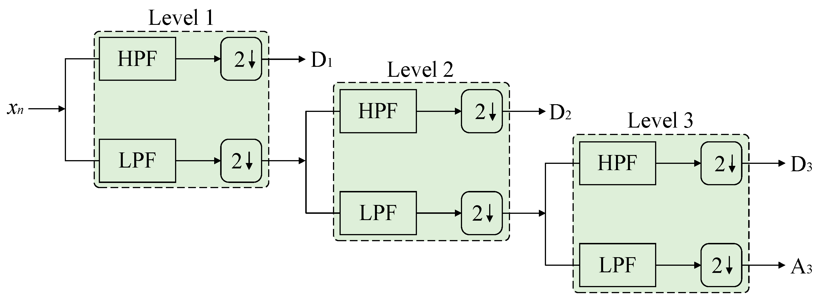
To meet the requirements of digital signal processing, the discrete wavelet transform (DWT) further discretizes the scale and translation parameters, decomposing the signal into multi-layer subbands of low-frequency approximate components and high-frequency detail components. Based on the fast implementation framework of the Mallat algorithm, the DWT performs downsampling and decomposition of the signal through the iteration of the filter bank, forming a hierarchical structure for multi-resolution analysis [44]. The structure of DWT is shown in Figure 4.

Each pair of filters consists of a high-pass filter (HPF) and a low-pass filter (LPF), followed by a downsampler to form a decomposition level, which, respectively, generates detail coefficients D and approximation coefficients A. Starting from the coefficients of the last level and arranging these coefficients in sequence, the DWT is formed. Since the frequency band of each level has been halved, the downsampling efficiency has been improved. Therefore, DWT has a high time resolution in the high-frequency band and a high-frequency resolution in the low-frequency band.

Sezgin et al. [45] proposed a time-frequency analysis method based on the mixture of DWT and complex exponential modulation. It shifts the target harmonic frequency band to the vicinity of the fundamental frequency through complex exponential modulation. And the high-precision characteristics of DWT in the low-frequency band are utilized for decomposition. It overcomes the problem of decreased accuracy caused by the increase of bandwidth in the high-frequency band in traditional DWT. In [46], an innovative method of compressive sensing empirical wavelet transform was proposed. This method first constructs an adaptive empirical wavelet filter bank based on spectrum segmentation. Then the compressive sensing algorithm is introduced. Finally, the time-domain wavelet coefficients are obtained by combining the inverse Fourier transform. It can achieve precise measurements of energy in each frequency band.

2.3. Adaptive Tracking Method

The adaptive tracking method realizes the online identification and tracking of time-varying signal characteristics by constructing a closed-loop parameter update mechanism. This type of method is driven by the dynamic characteristics of the signal and combines the theory of recursive optimization. By adjusting the model parameters or filter structure in real time, it can effectively overcome the defects of non-stationary signal spectral leakage and limited frequency resolution.

2.3.1. Kalman Filtering

Kalman filtering is an optimal state estimation technique based on linear minimum variance. It optimally estimates the state of the dynamic system through the state equation and observation equation of the system. It has wide applications in multiple fields [47]. Its state equation and observation equation are as follows:

$$\begin{array}{l}{x}_{k+1}=A x_k+w_k\\ z_k=H_k{x}_k+v_k\end{array}$$

(6)

where $x_k$ is the state vector; A is the state transition matrix; $w_k$ is the model error; $z_k$ is the observation vector; $H_k$ is the observation matrix; $v_k$ is the measurement error.

Kalman filtering estimates the system state through two steps: prediction and update. The prediction step predicts the state at the current moment based on the state estimation of the previous moment and the system model. The update step uses the current observations to correct the prediction results to obtain a more accurate state estimation. The classical Kalman filtering requires that both the dynamic model and the measurement model of the system have a linear relationship. If it is nonlinear, the model needs to be linearly approximated through the first-order Taylor series expansion.

The improved method based on dual Kalman filters proposed by Köse et al. [48] can break through the limitation of the traditional FFT fixed window and provide adaptive solutions for dynamic power quality analysis. An innovative method based on a two-stage adaptive symmetric strong tracking square root cubature Kalman filter was proposed in [49]. It can achieve precise dynamic tracking of interharmonics by integrating Root-Music high-resolution spectral analysis and the improved Kalman architecture.

2.3.2. Adaptive Notch Filter (ANF)

ANF is a frequency estimation method based on nonlinear dynamic systems. The core idea is to construct a filter with adjustable notch frequency and combine the error feedback mechanism to track the time-varying component frequencies in the signal. The core of ANF is a set of nonlinear differential equations, which adjust the notch frequency through error feedback:

$$\left\{\begin{array}{l}\ddot{x}+{\theta }^{2}x=2\zeta {\theta }^{2}e(t)\hfill \\ \dot{\theta }=-\gamma x{\theta }^{2}e(t)\hfill \\ e(t)=y(t)-\dot{x}/\theta \hfill \end{array}\right.$$

(7)

where x presents the state variable; $e\left(t\right)$ represents the error signal; $y\left(t\right)$ represents the input signal; θ represents the estimated frequency; $\zeta$ determines the depth of the notch and hence the noise sensitivity of the ANF; γ determines the adaptation speed and hence the capability of the ANF in tracking the frequency variations.

The improved algorithm proposed by Mojiri et al. [50] introduces a parameter adaptive mechanism and a frequency-domain decoupling strategy. The dynamic tracking of harmonics and interharmonic components at any frequency in power signals has been achieved. Meanwhile, it shows robustness in a noisy environment. In [51], an improved parallel adaptive notch filtering algorithm was proposed for the three-phase power system. It processes the three-phase signals, respectively, by constructing three dynamically coupled sub-filters and designs a unified frequency update loop. The joint estimation of the power grid frequency and its rate of change has been achieved.

2.4. Machine Learning Method

Machine learning is an emerging data-driven paradigm. It breaks through the dependence of traditional methods on explicit mathematical models by independently mining the nonlinear mapping relationship between signal characteristics and interharmonic parameters. Its core advantage lies in being able to extract universal laws from massive measured data and adaptively handle high dimensional signal features under complex working conditions. It provides a new methodological framework for the monitoring of interharmonics.

2.4.1. Adaptive Linear Element (ADALINE)

ADALINE is an adaptive filter used for noise cancellation or signal extraction [52]. Based on Equation (1), it is assumed that the waveform of the measured voltage or current in a power system with a known fundamental frequency $f_0$ is the sum of all harmonic components with unknown amplitudes and phase angles. The discrete form of the estimated signal $y\left(n\right)$ is as follows:

$$\begin{array}{ll}\hfill y(n)& ={\displaystyle \sum _{k=1}^K{A}_k\sin (2\pi k{f}_{0}n\Delta t+{\varphi }_k)}\hfill \\ & ={\displaystyle \sum _{k=1}^K(A_k\cos {\varphi }_k\sin 2\pi k{f}_{0}n\Delta t+A_k\sin {\varphi }_k\cos 2\pi k{f}_{0}n\Delta t})\hfill \\ & ={\displaystyle \sum _{k=1}^K({\alpha }_k\sin {\theta }_k+{\beta }_k\cos {\theta }_k)}\hfill \end{array}$$

(8)

where $A_k$ is the amplitude of the Kth harmonic; ${\varphi }_k$ is the phase angle of the Kth harmonic; k is the total number of harmonics; n is the sampling exponent; ∆t is the sampling interval.

It can be obtained from Equation (8):

$$\left\{\begin{array}{l}{\alpha }_k=A_k\cos {\varphi }_k\hfill \\ {\beta }_k=A_k\sin {\varphi }_k\hfill \\ {\theta }_k=2\pi k{f}_{0}n\Delta t\hfill \end{array}\right.$$

(9)

Equation (8) can also be written as follows:

$$y(n)=W^T(n)\cdot x(n)$$

(10)

includes

$$W(n)=\left[\begin{array}{c}{\alpha }_1\\ {\beta }_1\\ ⋮\\ {\alpha }_k\\ {\beta }_k\end{array}\right]x(k)=\left[\begin{array}{c}\sin {\theta }_1\\ \cos {\theta }_1\\ ⋮\\ \sin {\theta }_k\\ \cos {\theta }_k\end{array}\right]$$

(11)

where $W^T$ is the weight of ADALINE; $x\left(k\right)$ is the input vector of ADALINE.

The estimation error is minimized by the gradient descent method. The amplitude and phase angle of the Kth harmonic can be obtained through the following calculation:

$$A_k=\sqrt{{\alpha }_k^2+{\beta }_k^2}\hspace{1em}{\varphi }_k={\tan }^{-1}({\displaystyle \frac{{\alpha }_k}{{\beta }_k}})$$

(12)

where $-\pi \le {\varphi }_k \le \pi$.

An improved two-stage ADALINE structure was proposed by Chang et al. [53]. This method adopts the Prony spectrum estimation technique to dynamically track the frequency components of the signal in the first stage. In the second stage, the estimated frequency is fed back to the ADALINE network and the amplitude-phase parameters are updated through the recursive least square method. This cascading structure realizes the decoupled estimation of frequency and amplitude-phase parameters while maintaining real-time processing capabilities. In [54], a power quality disturbance detection method based on the collaborative work of ADALINE and the feedforward neural network (FFNN) was proposed. The interharmonic components are dynamically tracked through ADALINE, and the root-mean-square voltage and total harmonic distortion are calculated in real time. Combined with FFNN for the voltage waveform level, a multi-dimensional analysis framework integrating frequency-domain features and time-domain morphology was constructed.

2.4.2. Convolutional Neural Network (CNN)

CNN is widely used in the field of computer vision. This method is inspired by the human visual system, thereby endowing computers with the ability to recognize various patterns from pictures [55]. Its core structure is composed of convolutional layers, pooling layers and fully connected layers through function-oriented modular stacking. The basic structure of the classic CNN is shown in Figure 5.

The convolutional layer learns the feature representation of the input through convolution operations and nonlinear activation functions. Low-level features such as edges and curves can be extracted. The pooling layer adopts operations such as average pooling or maximum pooling. Translation invariance is achieved by reducing the resolution of the feature map to decrease the amount of data and retain important features. The fully connected layer connects all the neurons in the previous layer with each neuron in the current layer for advanced reasoning to generate global semantic information. The output layer is used for classification tasks, and it adopts methods such as the softmax operator or support vector machine. The optimal parameters are obtained by minimizing the loss function through methods such as stochastic gradient descent.

Severoglu et al. [57] proposed a deep learning framework based on CNN. This method designs a three-layer convolution-pooling structure and combines fully connected layer regression analysis. The high-precision extraction of interharmonic parameters in the scenario of fundamental frequency fluctuations has been achieved. A deep learning method based on the fusion of CNN and long short-term memory network was proposed in [58]. It innovatively integrates the functions of low-pass filtering and advanced prediction into a single network structure. Real-time prediction and compensation of interharmonics in electric arc furnaces can be achieved.

3. Suppression Strategies for Interharmonics

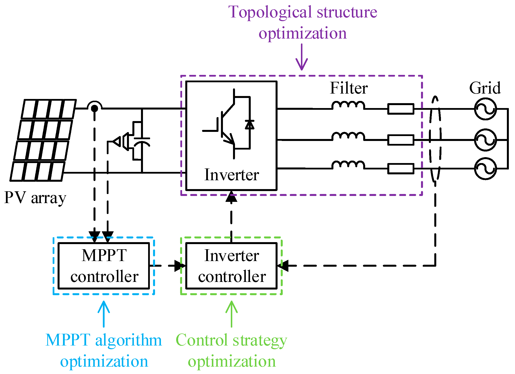
After understanding how to monitor the interharmonics, effectively suppressing the detected interharmonics has become a key issue. At present, there are mainly three types of interharmonic suppression strategies in grid-connected PV systems. This section will discuss them respectively starting from the MPPT algorithm optimization, control strategy optimization and topological structure optimization. The interharmonic suppression strategy based on the single-stage grid-connected PV system structure is shown in Figure 6.

3.1. MPPT Algorithm Optimization

The disturbance of the MPPT algorithm is mainly influenced by its disturbance step size and sampling rate. The disturbance step size determines the amplitude of the reference voltage adjustment each time. A larger disturbance step size will result in a more significant voltage step change. The disturbance step size has a significant impact on the amplitude of the interharmonic components. The sampling rate determines the frequency at which the MPPT algorithm performs perturbations, that is, the number of times the reference voltage may change within a unit of time. The sampling rate has an impact on both the amplitude and frequency of interharmonics. Therefore, the optimization of the MPPT algorithm mainly starts from two aspects: improving the perturbation step size and the sampling rate [59].

The specific optimization methods can be classified as follows: constant voltage MPPT algorithm, zero perturbation MPPT algorithm, variable step size MPPT algorithm and random perturbation frequency MPPT algorithm.

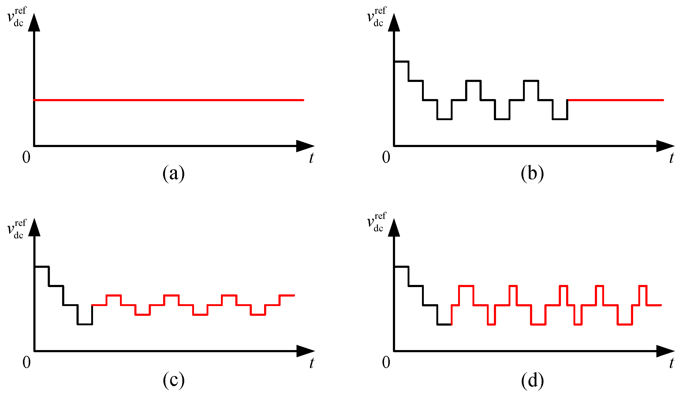
The constant voltage MPPT algorithm refers to performing MPPT under a constant DC voltage command without introducing perturbation. Since the system operates under a fixed DC voltage command, the interharmonics caused by the MPPT algorithm can be eliminated, thus having a better suppression effect. Moreover, the constant voltage MPPT algorithm also has the advantages of a simple principle and easy implementation. However, this method will reduce the tracking accuracy of MPPT and decrease the utilization rate of solar energy [9]. In actual operation, the voltage at the maximum power point of the PV system will fluctuate due to the dynamic changes in environmental temperature and the level of solar irradiance. Given this, the constant voltage MPPT algorithm applies to scenarios where PV inverters are in low-power operating conditions.

The zero perturbation MPPT algorithm refers to the situation where the DC voltage is detected to operate continuously for three three-point oscillation periods. It is regarded as having tracked the maximum power point, and then the perturbation step size is changed to zero. The interharmonics caused by the disturbance of the DC voltage command can be eliminated [60,61]. In the steady state, this method has the same interharmonic suppression effect as the constant voltage MPPT algorithm and does not reduce the tracking accuracy of MPPT. However, this method is unable to track the new maximum power point when the lighting conditions change slowly, resulting in a decrease in the tracking accuracy of MPPT. Therefore, the zero perturbation MPPT algorithm applies to scenarios where the solar irradiance is relatively stable.

The variable step size MPPT algorithm refers to the use of a larger perturbation step size for rapid tracking when the DC working voltage is far from the maximum power point. When it is detected that the system is operating near the maximum power point, small steps are used for perturbation [62]. This method does not have an impact on the dynamic performance of MPPT, but the suppression effect is relatively less obvious compared to the previous several methods. This method selects a compromise scheme between a faster MPPT speed and a better interharmonic suppression effect by dynamically adjusting the perturbation step size. It applies to scenarios with local shadow occlusion.

The random perturbation frequency MPPT algorithm refers to the dynamic random switching of the perturbation frequency between the fast perturbation frequency and the slow perturbation frequency [63]. The random change of the perturbation frequency can reduce the amplitude of the interharmonic current in general, and it will not affect the dynamic performance of the MPPT algorithm either. However, although this method can reduce the overall level of the amplitude of the interharmonic current, it will generate more frequencies of interharmonics, making the distribution of interharmonics more diverse. Furthermore, simply randomly processing the perturbation frequencies without exploring the influence of the arrangement of different perturbation frequencies on the interharmonics also restricts the application of this method.

Figure 7 shows the interharmonic suppression strategies for the MPPT algorithm optimization as mentioned above.

3.2. Control Strategy Optimization

In grid-connected PV systems, the dynamic response characteristics of the inverter control loop are the key factors for the generation of interharmonics. For this problem, the optimization of the control strategy can be improved in two aspects: the reshaping of the dynamic characteristics of the voltage loop and the collaborative optimization of the inverter controller.

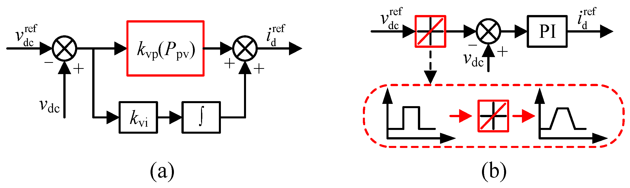
Sangwongwanich et al. [9] proposed two control methods for the voltage loop in PV inverter controllers: voltage loop adaptive gain control and voltage loop rate limiter. Both of these methods reduce the disturbance of the command value of the current loop by changing the dynamic characteristics of the voltage loop, thereby achieving the purpose of reducing interharmonics. The voltage loop adaptive gain control dynamically adjusts the proportional coefficient of the voltage loop controller according to the size of the power. The interharmonics are suppressed by reducing the dynamic response time of the voltage loop. The voltage loop rate limiter converts the step change of the DC voltage command into a ramp change, making the disturbance of the DC voltage command smooth. Both methods have a good suppression effect on interharmonics between high frequencies, but they will sacrifice the dynamic performance of the system. Figure 8 shows the interharmonic suppression strategies based on voltage loop optimization.

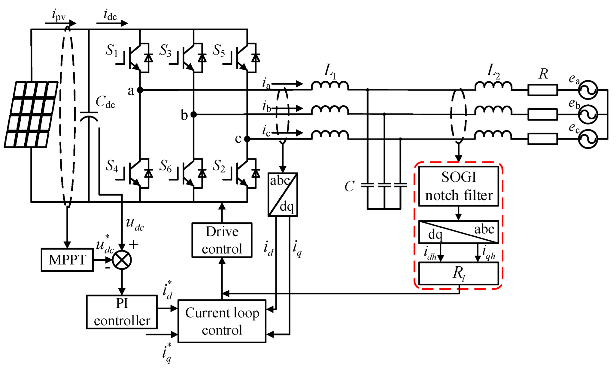
Some scholars have found that introducing additional virtual series impedance in the controlled power branch of the inverter can change the impedance characteristics of the system without increasing the power loss of the load [64]. It can improve the interharmonics generated by PV power generation systems. However, the introduction of virtual impedance will reduce the tracking performance of the system for the fundamental current of power frequency. Then, the second-order generalized integrator (SOGI) notch filter was introduced to extract other voltage and current components except for the power frequency, to achieve impedance reshaping. In [65], an interharmonic suppression strategy based on the SOGI virtual impedance method was proposed. Figure 9 shows the interharmonic suppression strategy based on the SOGI virtual impedance method.

Firstly, the interharmonic components of the current sampling values are extracted by using the SOGI notch filter. This current is transformed by abc/dq to obtain the d-axis interharmonic current $i_{dh}$ and the q-axis interharmonic current $i_{qh}$ in the synchronous rotating coordinate system. Then, these currents are fed back into the pulse width modulation (PWM) via the virtual impedance $R_l$ to reshape the impedance. It can effectively reduce the interharmonic content without increasing system losses. This method does not affect the current tracking accuracy and the MPPT tracking effect, but its implementation is rather complex.

By constructing the interharmonic cost function, Mao et al. [66] proposed a model predictive control (MPC) approach with an interharmonic suppression function. Aiming at the problem of reduced accuracy of the prediction model caused by DC voltage fluctuations, a voltage vector prediction strategy is introduced. It can update the output voltage vector of the inverter in real time based on the calculation of the predicted value of the DC voltage, improving the accuracy of the MPC. However, MPC is essentially a local optimization control method. It can only bring the system to the optimal state in a short time, but it cannot guarantee the stability of the system within a large time scale range, especially after adding the interharmonic cost function. If the fundamental following ability of the grid-connected current and the interharmonic suppression ability cannot be well balanced, it will be more likely to cause instability of the system. From this, the Lyapunov stability criterion was introduced to establish stability constraints. By determining the alternating switching state of the system, the system can operate more stably while achieving interharmonic suppression. Figure 10 shows its control strategy diagram.

Firstly, the MPPT employs the perturb and observe (P&O) to sample the DC voltage $v_{dc}$ of the inverter and the output current $i_{pv}$ of the PV array, and determines the position of the operating point, thereby outputting the DC voltage command $v_{dc}^{ref}$. Subsequently, the voltage loop outputs the d-axis current command $i_{dc}^{ref}$ through the PI controller. The dq-axis current command is transformed through coordinates to obtain the αβ-axis current commands $i_{\alpha }^{ref}$ and $i_{\beta }^{ref}$. Meanwhile, the output current $i_{acb}$ of the inverter is sampled and then transformed into coordinates to obtain the output current $i_{\alpha \beta }$ on the αβ-axis. Next, a two-step prediction model is used to predict the current values $i_{\alpha \beta }^{\ast }\left(k+1\right)$ and $i_{\alpha \beta }^{\ast }\left(k+2\right)$ at the next time instant. The amplitude of the interharmonic current is calculated by applying the orthogonality theorem of trigonometric functions. Based on this, a cost function that combines current tracking and interharmonic suppression is constructed. Then, the cost function is calculated for the predicted currents corresponding to the eight switch states of the inverter, and unstable switch states are excluded based on the Lyapunov stability condition. Finally, the stable switch combination with the lowest cost $\left(S_1~S_6\right)$ was selected to drive the inverter, thereby achieving the coordinated control of $v_{dc}^{ref}$ tracking and interharmonic suppression. This method does not affect the current tracking accuracy and the MPPT tracking effect, but is only applicable to P&O and incremental conductance (INC) algorithms.

3.3. Topological Structure Optimization

Due to the differences in application scenarios and power levels, grid-connected PV systems have diverse topological structures. By analyzing the operational characteristics of the specific topological structure and combining the generation mechanism of interharmonics. Corresponding suppression strategies can be formulated.

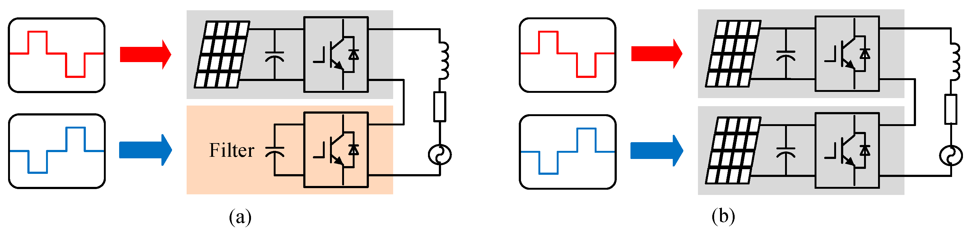
Some scholars have successively proposed the interharmonic filter [67] and the phase-shifting MPPT algorithm based on cascaded inverters [68,69] to suppress the interharmonic current of single-phase PV inverters. The former introduces an additional set of switch tubes as interharmonic filters for the cascade inverter. By controlling the DC voltage of the interharmonic filters, the total DC voltage is smoothed to suppress the generation of interharmonics. The latter performs phase-shifting processing on the DC voltage command of the cascaded inverter. It enables the DC voltage command disturbances of multiple inverters to cancel each other out, to achieve the purpose of suppressing interharmonics. Both of these methods have a good suppression effect on interharmonics across the entire frequency band. However, the former requires the introduction of an additional set of switch tubes, increasing the cost. The latter, although it does not have this problem, is only effective for the cascaded inverter topology. And the consistency requirements for the parameters and operating conditions of the cascaded inverter are relatively high. Figure 11 shows the interharmonic suppression strategies based on topological structure optimization.

4. Discussion and Outlook

After understanding the interharmonic monitoring methods and suppression strategies among various types. To better demonstrate their respective characteristics and applicability, this section will conduct a horizontal comparison and analysis of their advantages and disadvantages one by one. The comparison of the advantages and disadvantages of interharmonic monitoring methods is shown in

Table 2. Summary of interharmonic monitoring methods.

Categories	Methods	Advantages	Disadvantage	Computational Complexity	Real-Time Computing	Applicable Scene
Parametric method	ESPRIT [23,24,25,26]	High-frequency resolution No need for the assumption of signal periodicity	Poor anti-noise ability	High	Poor	Non-stationary signal
	Prony [27,28,29,30]	The signal can be fitted as an exponential function	Poor anti-noise ability	High	Poor	Non-stationary signal
	MPM [31,32,33]	High-frequency resolution	Rely on model order estimation	High	Poor	Low signal-to-noise ratio situation
Non-parametric method	Fourier transform [34,35,36,37,38,39,40,41]	Fast and efficient calculation	Spectral leakage and fence effect Poor adaptability in time-varying signals	Low	Good	Periodic stabilization signal
	Wavelet transform [42,43,44,45,46]	Adaptively select basis functions	The frequency resolution varies in different frequency bands	High	Poor	Time-varying non-stationary signal
Adaptive tracking method	Kalman filtering [47,48,49]	Strong anti-noise ability	Rely on the model Sensitive initial value selection	High	Middle	Dynamic system state estimation
	ANF [50,51]	Simple in structure	Low-frequency resolution Slower signal frequency mutation response	Low	Good	Real-time slowly varying signal
Machine learning method	ADLINE [52,53,54]	Adaptive learning ability	Sensitive initial weight selection	High	Middle	Low-order nonlinear slowly varying signals
	CNN [55,56,57,58]	Strong signal feature capture capability	High training costs	High	Poor	Complex feature extraction

.

Parametric methods usually have the advantage of high-frequency resolution and can analyze signal components more accurately under certain conditions. However, such methods are often accompanied by relatively high computational complexity. This leads to a relatively long data processing time and poor real-time performance. It is difficult to meet the demand for real-time monitoring of rapidly changing signals. It is applicable to scenarios where there is a high demand for monitoring the accuracy of interharmonic frequencies and amplitudes.

In the non-parametric methods, the Fourier transform has the advantages of a simple principle and easy implementation. However, it has problems such as spectral leakage and limited resolution, which often lead to low estimation accuracy of the interharmonic frequency and amplitude of non-stationary signals. Therefore, it is usually used for the interharmonic analysis of steady-state signals. In contrast, the wavelet transform has the ability of multi-resolution analysis. It can analyze signals at different time scales and is suitable for interharmonic analysis in non-stationary signals.

In the adaptive tracking methods, the Kalman filter is based on the state space model and can effectively track the dynamic changes of interharmonic signals in a noisy environment. Therefore, it is suitable for scenarios where the signal is disturbed by noise. ANF can adaptively adjust the notch frequency according to the signal characteristics and suppress the interharmonic interference of specific frequencies in real time. It performs better in terms of real-time performance and is suitable for processing interharmonic signals with variable frequencies.

In the machine learning methods, the ADALINE network has the characteristics of a simple structure and fast training speed, and has a certain ability to process interharmonic signals in nonlinear systems. However, there are certain limitations in the extraction of complex signal features, and it is generally applicable to the real-time estimation of stationary signals. With a multi-layer convolution structure, CNN can automatically extract the deep features of interharmonic signals and has higher accuracy in feature recognition and classification tasks. However, its training process requires a large amount of data support, and the model training time is relatively long. It applies to the classification and monitoring of complex interharmonic data.

To sum up, various interharmonic monitoring methods show distinct technical differences and application characteristics. To break through the limitations of a single method. Some scholars have actively explored the path of cross-integration and constructed a new type of hybrid monitoring method through complementary advantages.

Bracale et al. [70] proposed an interharmonic estimation method combining sliding window ESPRIT and DFT. Firstly, the fundamental components are estimated with high precision by using the sliding window ESPRIT. Then, the harmonics are analyzed through the synchronized DFT. Finally, the residual signal is processed by ESPRIT to obtain the interharmonic parameters. This method improves the analysis efficiency of interharmonics through a staged processing strategy. Aiming at the limitations of the traditional DFT method in processing time-varying signals, Oliveira et al. [71] constructed a mixed-signal processing model by combining Prony’s method and Kalman filtering. The most appropriate time window length was determined by using statistical analysis, thereby improving the accuracy of interharmonic quantization.

After analyzing the monitoring methods of interharmonics and their advantages and disadvantages. For the detected interharmonic components, the following discussion will focus on the interharmonic suppression strategies. The advantages and disadvantages of the interharmonic suppression strategy are compared as shown in

Table 3. Summary of interharmonic suppression strategies.

Representative Research Cases	Advantages	Disadvantages
Constant voltage MPPT algorithm [9]	Good suppression effect Easy to implement	Lower utilization rate of solar energy
Zero perturbation MPPT algorithm [60,61]	Good suppression effect under steady state	The tracking accuracy of MPPT decreases under the slow change of illumination
Variable step size MPPT algorithm [62]	Does not affect the dynamic performance of MPPT	Relatively inconspicuous suppression effect
Random perturbation frequency MPPT algorithm [63]	Does not affect the dynamic performance of MPPT	Richer interharmonic frequency distribution
Voltage loop adaptive gain control [9]	Good suppression effect on high-frequency interharmonics	Reduce the system’s dynamic response speed Limit MPPT perturbation frequency
Voltage loop rate limiter [9]	Good suppression effect on high-frequency interharmonics	Reduce the system’s dynamic response speed
SOGI virtual impedance method [64,65]	Does not affect the current tracking accuracy and the MPPT tracking effect	Relatively complex to implement
MPC method [66]	Does not affect the current tracking accuracy and the MPPT tracking effect	Only applicable to P&O and INC algorithms
Interharmonic Filter [67]	Good suppression effect on interharmonics across the entire frequency band	Introduce an additional set of switch tubes Higher cost
Phase-shifting MPPT algorithm based on cascaded inverters [68,69]	Good suppression effect on interharmonics across the entire frequency band No additional switch tubes	Only effective for cascaded topology Have high requirements for the consistency of parameters and operating conditions

.

After clarifying that the disturbance of the DC voltage command output by the MPPT algorithm is the main source of interharmonics in grid-connected PV systems. The optimization of the MPPT algorithm can be directly taken as the entry point, and the corresponding interharmonic suppression strategy can be proposed. This type of method addresses the interharmonic problem from the root cause and therefore generally has a good interharmonic suppression effect. However, it may affect the tracking effect of the MPPT algorithm, such as reducing the tracking accuracy or affecting the dynamic performance.

Control strategy optimization achieves the purpose of indirectly suppressing interharmonics by improving the tracking behavior of voltage or current. Because it does not make adjustments to the MPPT algorithm, it overcomes the drawback that MPPT algorithm optimization methods affect the tracking effect of MPPT. However, it has problems such as a relatively insignificant suppression effect and a rather complex implementation process.

Topological structure optimization proposes corresponding interharmonic suppression strategies for specific topological structures. Because it needs to fully consider factors such as the characteristics, parameters and operating conditions of the topological structure, it can only play an effective role in systems with specific topological structures. Therefore, its application scope is relatively limited.

In the field of interharmonic monitoring, some scholars have significantly improved the accuracy and reliability of monitoring by combining different types of monitoring methods [70,71,72,73]. By contrast, in the research on interharmonic suppression strategies, most of the current literature only conducts analysis from a single optimization aspect [59,60,61,62,63,64,65,66,67,68,69]. No study has attempted to integrate multiple suppression strategies yet. Looking forward to the future, it is expected that some scholars can break through the existing framework and explore interharmonic suppression strategies from multiple dimensions. A better suppression effect can be achieved through the cross-fusion of multiple optimization methods.

5. Conclusions

With the large-scale grid connection and operation of PV systems, many power quality problems have emerged. Among them, the interharmonic problem has brought great challenges to the safe and stable operation of the power system. This paper classifies and summarizes the monitoring methods for interharmonics, and conducts an analysis of their respective advantages and disadvantages as well as a discussion on their applicable scenarios.

Regarding the detected interharmonics, this paper discusses them from three aspects, respectively: (1) The optimization based on the MPPT algorithm solves the interharmonic problem from the root. It can achieve a better suppression effect, but it will affect the tracking effect of MPPT to a certain extent. (2) The optimization based on a control strategy can avoid this, but the implementation of this strategy is rather complex and the suppression effect is relatively limited. (3) The optimization based on topological structure not only does not affect the tracking performance of MPPT but also achieves a better suppression effect. However, it needs to formulate different suppression strategies according to different topological structures, so its application scope is relatively limited.

In the future, it is expected that some scholars will continue to research suppression strategies from these three aspects. Meanwhile, it is hoped that some scholars can combine the advantages of these several types of optimization strategies to propose more comprehensive suppression strategies.