Article

Practices and Considerations in Wind Data Processing for Accurate and Efficient Wind Farm Energy Calculation

by
Angel Gaspar Gonzalez-Rodriguez
1,*,
Jose Manuel Riega-Medina
2,†,‡,
Ildefonso Ruano-Ruano
3,‡ and
Jose Vicente Muñoz-Diez
1,‡
1
Department of Electronic Engineering and Automation, University of Jaen, 23071 Jaen, Spain
2
Facultad de Ciencias, Universidad Nacional de Ingeniería, Rimac 15333, Peru
3
Department of Telecommunications Engineering, University of Jaen, 23071 Jaen, Spain
*
Author to whom correspondence should be addressed.
Current address: Higher Polytechnic School, University of Jaen, Campus las Lagunillas s/n, 23071 Jaen, Spain.
These authors contributed equally to this work.
Energies 2025, 18(13), 3402; https://doi.org/10.3390/en18133402 (registering DOI)
Submission received: 28 May 2025 / Revised: 16 June 2025 / Accepted: 19 June 2025 / Published: 27 June 2025
(This article belongs to the Special Issue Advancements in Wind Farm Design and Optimization)

Abstract

An accurate estimation of future wind conditions is essential for calculating the annual energy produced by a wind farm. This estimation should be based on historical wind data collected over several years at the site location. However, research articles often rely on data grouped into 12 sectors. This article examines five methods to improve the speed and accuracy in the use of wind data. First, it studies the effect of inadequate Weibull parameter calculation based on historical data showing that purely mathematical fitting methods (the traditional ones) are not valid. Then, the error introduced by wind speed discretization is evaluated showing that the traditional binning of 1 m/s is not always the best choice. Next, the effect of using symmetric wind roses is examined, demonstrating that it is possible to reduce computation time by half for layouts exhibiting point symmetry, with negligible error for other layouts. After that, the effect of abrupt wind condition distributions caused by sectorization, which can alter results when searching for optimal configurations, is analyzed proposing continuous interpolation of wind data to improve result consistency. Finally, an alternative to the wind rose is proposed to provide a quick assessment of the highest-quality wind directions.

1. Introduction

There are numerous factors that influence the viability of a wind farm project. While issues such as environmental impact on local flora and fauna, noise emissions, or visual intrusion can ultimately lead to the rejection of a project, it is primarily the economic aspects that determine a developer’s interest in installing a wind farm at a given site. The first factor considered when evaluating a site for a wind farm is wind speed—not only the average speed but also how frequently different wind speeds occur. Secondly, the distribution of wind direction also plays a key role in defining the relative positioning of the turbines, aiming to maximize the energy output while minimizing the detrimental effects of turbulence caused by wake interactions.
Consequently, the accurate estimation and processing of wind speed and direction data are critical for maximizing energy sales revenues.
The following data and variables are required or used for the estimation of the Annual Energy Production (AEP): the number of turbines (nt); the wind direction, in deg ( θ ); the free stream wind speed in m/s (u); the wind speed in m/s at turbine t taking into account wake effect ( v t * ); the electric power given by the turbine manufacturer’s power curve (Pc); and the density of probability at wind direction θ and wind speed v ( fr ( θ , u ) ). With them, AEP is obtained by adding the energy, E i produced by each turbine i, for all θ and for every u between the cut-in speed (uci) and thecut-out speed (uco). For a year ( T y = 8760 h ), the AEP can be expressed as [1] follows:
AEP = t = 1 n t E t = T y t = 1 n t u c i u c o 0 360 P c ( v t * ) fr ( θ , u ) d u d θ .
In this expression, the power produced by a turbine t of the array depends on the effective speed of the air flow that reaches the t-th turbine, v t * . Due to the wake effect, this effective speed is smaller than the free-flow air speed, u. There are different methods to estimate the wind speed deficit caused by wakes, of which the preferred is the Park or Jensen model, as indicated in [2]. The formulation of this model can be found in [3].
In general, the expression (1) is not analytically integrable. Therefore, it must be discretized, transforming the integrals into summations. Using wind direction bin size in deg ( δ θ ) and wind speed bin size in m/s ( δ u ) for the discretization, it yields the following.
AEP = T y t = 1 n t u B u θ B θ P c ( v t * ) fr ( θ , u ) δ θ δ u .
or expressed as average power
P a v = t = 1 n t u B u θ B θ P c ( v t * ) fr ( θ , u ) δ θ δ u .
where B u and B θ are, respectively, the sets of speed bins and directions bins, i.e.,
B u = u i | u i = u ci + i δ u , i { 0 , 1 n b u 1 } with n b u = u co u ci δ u + 1
B θ = θ j | θ j = j δ θ , j { 0 , 1 n b θ 1 } with n b θ = 360 δ θ
The most realistic way to evaluate the AEP is by using a historical time series of wind data (speed and direction) over a given period. However, since this type of input data is difficult to handle directly, researchers usually prefer to describe wind conditions through a sector-based classification. This approach provides the frequency of wind occurrence in each sector (forming the wind rose), along with the probability density function of wind speeds within each sector (typically a Weibull distribution).
As can be seen, the concept of a sector, which is more commonly associated with the description of wind data, is not inherently related to the concept of a direction bin, which is used for the discretization in AEP calculations. Nevertheless, many authors tend to confuse these terms. Assuming a certain number of sectors (ns), then a sector ς s , of sector size ( Δ θ ), is defined as the interval
ς s = [ ( s 0.5 ) Δ θ , ( s + 0.5 ) Δ θ ) with s = 0 n s 1 and Δ θ = 360 n s
Furthermore, it is common to establish the convention that angle 0 is placed at North and angles increase in a clockwise direction.
There are works that have developed various improvements to speed up this calculation [4], although they deviate from the structure of this formulation by introducing structural modifications in the evaluation of interactions between turbines.
In this work, five different techniques to increase the accuracy and speed of the calculation of AEP will be studied, without substantial modifications to expression (2), but rather focusing on the evaluation and treatment of fr ( θ , u ) and δ u and/or Δ θ .
In this article, the existing literature on each of the five topics will be reviewed, and new ideas will be presented that lead to methods or approaches different from the traditional ones. For each of the five topics, a review of the state of the art, methodology, results, and discussion will be included in the following sections:
  • Section 2 analyses the traditional method for the estimation of the Weibull parameters and proposes a new procedure to derive them.
  • Section 3 explores the effect of wind speed binning on AEP calculation, concluding that the traditional speed binning of 1 m/s is not always the best choice for accuracy nor speed.
  • Section 4 demonstrates that is possible to halve the number of calculations for symmetrical wind farm layouts for any layout type (with minimal error).
  • Section 5 shows that the traditional preprocessing of wind conditions into 12 sectors leads to inconsistent results and proposes a sectorization with a higher number of sectors. If historical data are not available, wind data should be interpolated to increase the number of sectors.
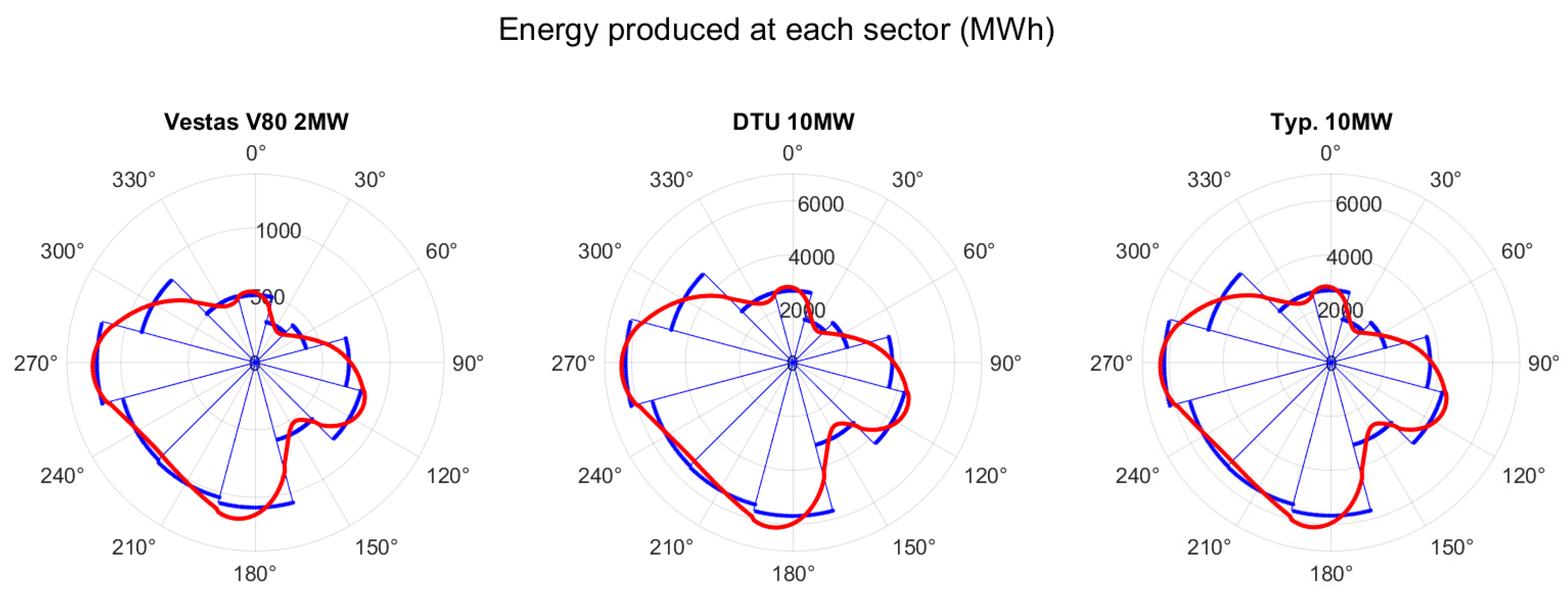
  • Section 6 presents an alternative visualization of wind resource potential, using a one-dimensional plot to illustrate the expected energy output from each direction.

Input Data

For the analyses carried out in this work, data from different sources have been compiled regarding the characteristics of various wind farms (all of them offshore). These data are available in [5] and are as follows:
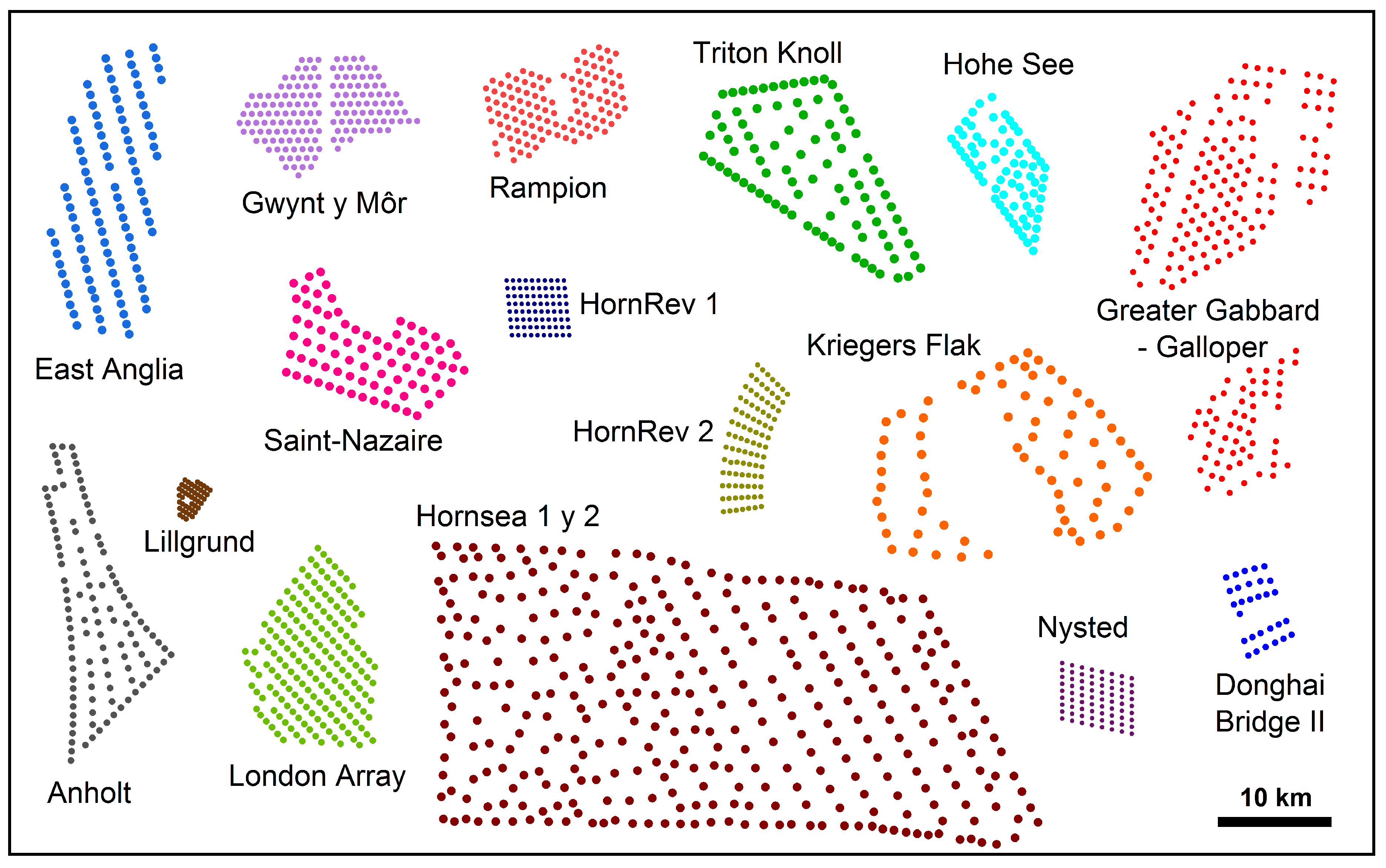
  • General characteristics of the wind farms. Found in the Excel file
    Offshore Wind Farms.xlsx, which includes data from 28 offshore wind farms.
  • Concession areas. Contained in the file concession_area.m.
  • Turbine positions at each wind farm. Contained in the file position_turbines.m.
  • Turbine curves. Curves for power and Power factor (Cp), and when available, also for Ct, found in DataTurbines.m.
Additionally, the file WindData_MERRA2.zip includes a series of files obtained from the MERRA-2 Demo website (Modern-Era Retrospective analysis for Research and Applications), which estimate wind conditions at different offshore wind farms. As input to the application, the coordinates closest to each studied wind farm were provided, and data were retrieved from 1 January 2004, to 31 December 2006, with measurements every 10 min, resulting in 157,825 instances. This frequency is equal to the one established in IEC 61400-12-3 [6] for the measurement based site calibration. The reference height was 10 m, and the provided wind speed values were adjusted using the following formula to compute the wind speed at hub height z b :
V z = V 0 ln ( z b / z 0 ) ln ( z r / z 0 )
with z r = 10 m and z 0 = 0.001 m, which is the roughness length for a sea surface with moderate wave conditions.

2. Deducing the Optimal Weibull Parameters from Time Series Data

2.1. Introduction and State of the Art

As previously anticipated, the two-parameter Weibull distribution is usually associated with all wind directions within the same sector, where it is necessary to calculate scale factor of the Weibull distribution (A) and shape factor of the Weibull distribution (k) for each sector. However, the vast majority of studies use purely statistical methods, without considering their use as an energy source.
Serban et al. [7], based on wind speed data recorded by two meteorological stations, calculated the wind power density and concluded that the Weibull distribution is the most suitable model for the recorded wind data. Singh et al. [8] list ten methods for obtaining these parameters and apply them to two sites, revealing significant differences in the estimations provided by the methods, particularly in k. Chaurasiya et al. [9] also compare the estimations given by nine methods for data series collected at heights of 80 m and 100 m over the course of one month, using a cup anemometer and two remote sensing techniques (SODAR and LiDAR). El-Bshah et al. [10] estimate the Weibull parameters based on real wind speed data collected over a five-year period and validate their results using three performance evaluation metrics (R2, RMSE, and COE).
A more physical approach, which exploits the dependence of wind power on the cube of wind speed, is provided by the energy pattern factor method for the estimation of k [11]. This method is extended in [12] to also estimate A.
This idea will be exploited using a generic Pc for the estimation of the most appropriate Weibull parameters.

2.2. Method

Note: the code and input data to replicate this study can be obtained from [5] in the WeibullFitting folder.
Currently, to estimate the energy production of a wind turbine at a specific location, two methods can be used:
  • Histograms based on historical data: This method starts with a database containing measurements of wind direction and speed taken every ten minutes, following the IEC 61400-12-2:2022 standard [13]. During data processing, the measurements are grouped into bins for both wind speed and wind direction. Regarding wind speed, the wind speed bins typically have a size δ θ = 0.5 m/s as indicated by the IEC 61400-12-1:2022 standard, or 1 m/s as is common in research studies [14]. For the wind direction, greater representativeness of the wind conditions is achieved by grouping every 1 deg, although the IEC 61400-12-3:2022 standard specifies a bin size Δ θ = 10 deg. At the final stage of the data processing, a matrix fr h ( θ , u ) is filled with the frequency of occurrence for each wind direction and speed interval, with u B u and θ B θ defined in (4) and (5), respectively.
    The expression for the AEP, adapted from (3) is
    AEP h = T y t = 1 n t u B u θ B θ P c ( v t * ) fr h ( θ , u ) δ θ δ u .
    or, expressed as average power
    P a v h = AEP h T y = t = 1 n t u B u θ B θ P c ( v t * ) fr h ( θ , u ) δ θ δ u .
    This method is appropriate when historical data is available. However, most existing research studies do not have access to such detailed data for the site under study.
  • Wind condition sectorization and Weibull distribution fitting by sector: this method starts by dividing the polar map into ns sectors, typically 12. Then, a two-parameter Weibull distribution is fitted to best represent the frequency of occurrence of each wind speed within each sector. This method results, on one hand, in a wind rose with ns sectors showing the frequency of wind occurrence per sector, and on the other hand, it provides the A and k values of the Weibull distribution fitted for each sector. This description of historical data is very manageable and is preferred by researchers, despite being less representative of reality.
    By defining the probability that the wind comes from sector s, given by the Windbull distribution ( fr s Wb ( u ) ) and the probability that the wind comes from sector s, given by the wind rose ( fr s wr ) as
    fr s Wb ( u ) = k s A s · u A s k s 1 exp u A s k s
    fr s wr = u 0 θ ς s fr h ( θ , u ) .
    the expression for the estimated average power yields
    P a v W b = t = 1 n t u B u θ B θ P c ( v t * ) fr s Wb ( u ) fr s wr   δ θ δ u
    s = θ Δ θ
    where · is the ceiling of · and allows for the deduction of the sector s to which the wind direction θ belongs.
Regarding this second method, there are mathematical tools available that estimate the Weibull parameters from a historical dataset by counting the number of occurrences of each wind speed. For instance, the Matlab R2022b library includes a function (wblfit) that uses a gradient-based optimization method for maximum likelihood estimation (MLE) of these two parameters which will be referred to as A M L E and k M L E .
In the following, it will be shown that this fitting method, based purely on mathematical tools, leads to estimations that deviate from those obtained using direct historical data. As a first approach, an isolated turbine will be assumed, implying that there is no velocity deficit due to wake effects ( v t * = u ), hence (3) can be written as
P a v 1 = u B u P c ( u ) fr ( u ) δ u .
and specifically applied to the histogram and sector-wise Weibull fitting methods yield, respectively,
P a v h , 1 = u B u θ B θ P c ( u ) fr h ( θ , u ) δ θ δ u
P a v W b , 1 = u B u s = 1 n s P c ( u ) fr s Wb ( u ) fr s wr   δ u .
Instead of using a mathematical fit to the historical data, a sweep is proposed for different values of A and k so that the result of applying (12) and (16) closely matches (15). These values will be referred to as A s w and k s w ( s w for sweep). If the turbine model is defined, the turbine’s P c ( u ) is simply used in (12), and for each sector s, the A s and k s from (10) that minimize | P a v h , 1 P a v W b , 1 |  in each sector are obtained.
If the turbine model is not defined, e.g., because multiple types are being evaluated, this work proposes performing a sweep to fit the Weibull parameters that minimize the deviation | P a v h , 1 P a v W b , 1 |  for a turbine with a typical Pc, which is obtained by averaging the Pc curves of 17 turbines. It is worth noting that these turbines are pitch-controlled. For a turbine with a different technology, such as stall-controlled turbines, a different reference curve should be used. The reference power curve is presented in Table 1, and the code used to generate it can be obtained from [5] (file DataTurbines.m). The other power curves used for this study can also be found in the same file.

2.3. Results

In this way, starting from a time series of data corresponding to Anholt and provided in [5] (WindData_MERRA2.zip), the Weibull parameters that minimize | P a v h , 1 P a v W b , 1 |  have been obtained. Table 2 presents these parameters using MLE optimization, along with the data resulting from the sweep. Note that for consistency, wind data estimated by MERRA-2 has been used following the procedure described in Section 1, although more direct measurements can be found in [15].
Using the values from Table 2, | P a v h , 1 P a v W b , 1 |  has been calculated for four turbine models and for each of the twelve sectors, where the corresponding power curve was applied in equations (15) and (16). The models are as follows: Siemens Gamesa SWT-3.6-120 (Siemens Gamesa Renewable Energy S.A., Zamudio, Spain) with 3600 kW, Vestas V112/3450 (Vestas Wind Systems A/S, Aarhus, Denmark) with 3450 kW, Vestas V164-8.0 with 8000 kW, and the DTU reference turbine with 10 MW. Figure 1 shows these errors in the average power per sector, multiplied by the wind frequency in each sector ( fr s wr ). Lower errors in power estimation using the proposed method can be observed for all of the tested turbines. This same information for each sector is presented in Table 3, although recovering the sign in the error. Since the power P a v h , 1 is taken as true and therefore as the reference, the error P a v h , 1 P a v W b , 1 will be positive when the value of P a v W b , 1 is lower than the reference (i.e., power underestimation). By analyzing the sign of the errors, it is observed that the statistical fitting (using MLE) leads, in general, to positive values indicating an underestimation of the power. The last column shows the root mean square value of the weighted error, with lower values for the estimation power using the proposed sweeping method with an average power curve. Notably, the excellent agreement for the DTU reference turbine (as well as for the V112) suggests that its design may have been derived from the average characteristics of other commercial turbines.
In the file WR-Param.xlsx from [5], the Weibull parameters obtained using the proposed method are listed for the sites of thirteen offshore wind farms (OWFs). They are the result of launching the script Get_Weibull_All.m.

2.4. Conclusions

The statistical fitting (using MLE) of the Weibull parameters leads, in general, to an underestimation of the energy production. A more accurate estimation is obtained by performing a parameter sweep based on a typical power curve (e.g., DTU Reference 10 MW or the one from Table 1).

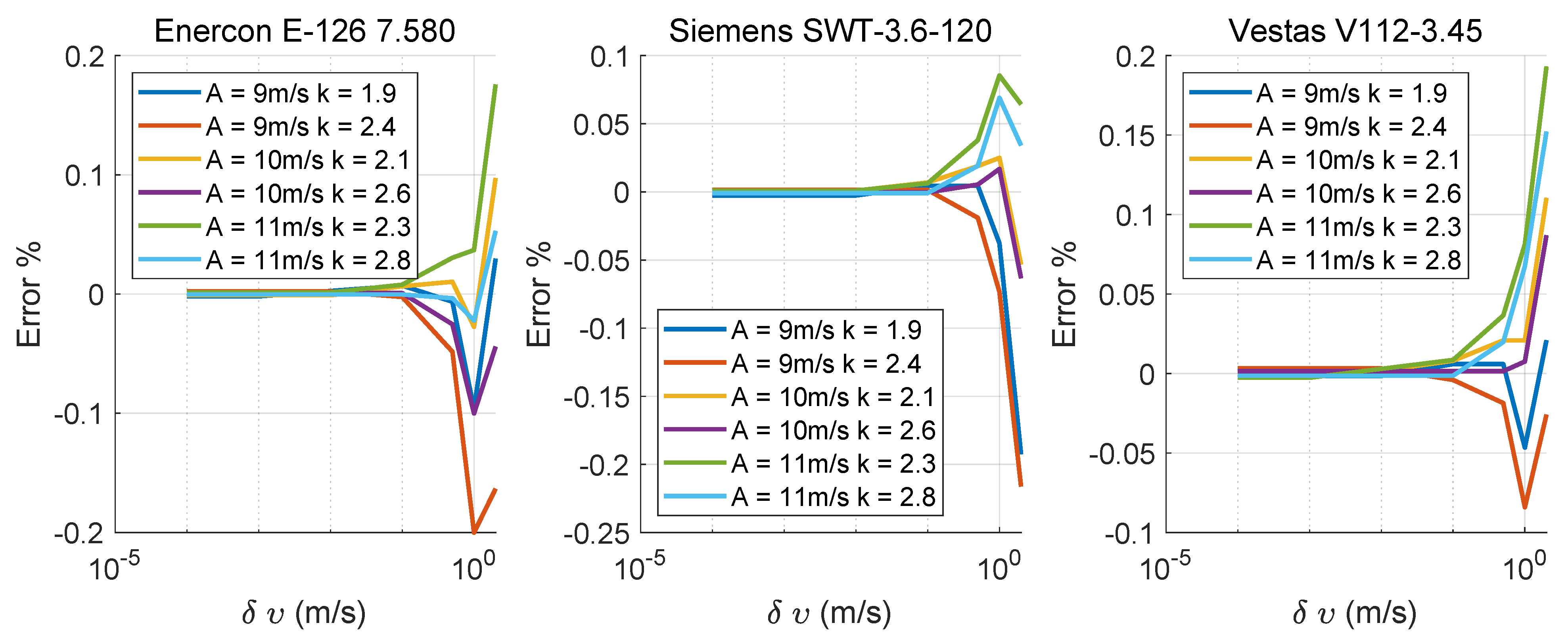
3. Effect of Wind Speed Binning on AEP Calculation

3.1. Introduction and State of the Art

In general, the calculation of the Annual Energy Production (AEP) of a wind farm typically relies on a wind speed discretization of 1 m/s, a convention established since the early studies on wind energy [16]. This approach is reflected in [14], which reviews 24 studies on this topic and finds that the majority of authors (19 out of 24) use this binning size, although other discretization intervals (0.5 m/s and 2 m/s) have also been investigated. It is worth noting that IEC standard 61400-12-6 [17] specifies a 0.5 m/s interval for the classification of data obtained from meteorological stations. The same interval is used in IEC standard 61400-12-1 [18] for the characterization of the wind turbine power curve. In other cases, to reduce the computational time (CT), they limit the study to a small number of test speeds [19], although this calculation is logically far from the real value and would only be useful for testing search algorithms.
In the following, the error introduced when using an overly coarse δ θ in Equations (2) and (4) will be studied.

3.2. Method

[Note that the script to reproduce this experiment is available in the repository [5], files Main_DiscretizationError_SizeBinSpeed.m and Errors_with_gamma.m].
As mentioned, expression (1) is not analytically integrable, and must be discretized. Using a non-infinitesimal value for the wind speed increments binws will cause an error when adopting the Equation (3). The IEC 61400-12 standard establishes the so-called bin method when a discretization of wind speed is required. Although the value specified in this standard is 0.5 m/s, it was previously mentioned that the authors prefer a wind speed bin size of 1 m/s [14]. Reducing this size will decrease the discretization error when using (3), though it will increase the number of operations of this calculation, which is typically the most time-consuming task when performing any type of optimization.
In [16], the following expression is proposed for the evaluation of a wind turbine, assuming a Weibull distribution for the wind speed and δ u = 1 m/s:
P a v = i = 0 n b i n s 1 p i e α i k + p i + 1 p i α i + 1 α i G ( α i + 1 , k ) G ( α i , k ) p i + 1 e α i + 1 k where p i = P c ( u i ) α i = u i A
u i defined in (4) and G obtained from the Gamma function Γ and the incomplete lower gamma function γ
G ( α , k ) = 1 k Γ 1 k γ 1 k , α k .
However, studies that estimate the mean power of a turbine, the total power of the wind farm, or equivalently the AEP, commonly use the simplified expression given in (3). In the following, the error resulting from using this simplified expression, as compared to the result obtained with (17), is analyzed for different values of δ u . For a clearer explanation, an isolated turbine will be assumed, implying that there is no velocity deficit due to wake effects ( v t * = u ) and there is no need to classify the wind directions in sectors, hence (3) can be written as (14), i.e.,
P a v = u B u P c ( u ) fr ( u ) δ u
If a Weibull distribution is considered for the fr ( θ , u ) , it will adopt the following form
fr ( u ) = k A · u A k 1 exp u A k

3.3. Results

In order to find out the influence of the δ u in the accuracy of the power calculation, the expression (14) has been used with different δ u (0.0001, 0.001, 0.01, 0.1, 0.5, 1 and 2, all in m/s). The experiments have been repeated with three different wind turbines, and six different wind conditions. The results are represented in Figure 2 showing the error obtained when using (14) for different δ u with regard to the estimation made with (17). As can be seen, not a clear inaccuracy is obtained if δ u = 2 m/s is used with respect to δ u = 1 m/s, which is the usual value. This is not the case of δ u = 0.5 m/s, which, in all cases yields more accurate estimations than δ u = 1 m/s. For this value of δ u , the error with respect to the values obtained from (17) is, in all cases, lower than 0.05%, and in most cases lower than 0.02%.
In addition to these comparisons, expression (17) has been tested, not only with δ u = 1 m/s, but also with δ u = 0.5 m/s and δ u = 2 m/s. The same results for the mean power production were obtained using 0.5 m/s and 1 m/s, with half of the CT for 1 m/s. When using 2 m/s, a very small error (in the order of 0.05%) appeared, with no improvement in computation time, which is an illogical outcome that requires further investigation.

3.4. Conclusion and Discussion

It is worth mentioning that, despite the apparent complexity of Equation (17), most of the calculations can be performed offline and stored in a look-up table, so that this method barely increases the CT.
For more accurate calculations, it is recommended to use Equation (17) with a bin size of δ u = 1 m/s, or Equation (19) with a discretization δ u no greater than 0.5 m/s. Logically, the CT is inversely proportional to the speed bin size.
In algorithms that require a large number of evaluations, where precision requirements are often relaxed, Equation (19) can be used with δ u = 1 m/s or even 2 m/s. However, it is advisable to first perform an analysis like the one shown in Figure 2, in order to assess the associated error.

4. Exploiting Symmetrical Layouts to Accelerate the AEP Evaluation

4.1. Introduction and State of the Art

With the proliferation of OWFs, the number of farms with regular structures is growing significantly. In [20], various cases of OWFs are shown with regular layouts, while also listing the advantages of such configurations in terms of maintenance operations, land footprint reduction, and navigation safety issues.
Ghaisas and Archer [21] employed a geometric approach and the regular arrangement of turbines to identify the directions in which the turbine rows should preferably be oriented. A similar study was carried out by Al-Yahyai et al. [22] to deduce an initial layout in an optimization process, thereby achieving a reduction in computation time. Neubert et al. [23] also used symmetrical layouts to speed up an optimization algorithm, with minimal impact on the result in terms of AEP. Both works also aim to improve the visual appearance of the installation.
Other authors [24] indicated that symmetric wind farm designs can generate slightly more energy than asymmetric distributions. However, although the differences may be positive or negative, there is generally no significant variation in terms of AEP between enforcing symmetry constraints or not [20].
In any case, the aforementioned works use symmetry as a constraint to reduce the number of possible solutions to be evaluated. A different approach is presented by Van Der Laan et al. [25], who listed the different types of symmetry that wind farms can adopt and demonstrated how the symmetry (rotational or mirror) of wind farm design can reduce the computational effort required to calculate the annual energy production as well as decrease the number of wind directions needed for the calculation. This can also be found in the PyWakeEllipSys documentation.
The point symmetry is a particular case of rotational symmetry, where the angle of rotation is 180 deg. For this case, a formal demonstration of the possibility to halve the number of calculations required to evaluate the AEP can be found in [15].
In the following, the formal conditions that allow the evaluation of only half of the wind directions in the AEP calculation will be reviewed. In the case of layouts without this symmetry, it will be shown that, although not formally demonstrated, computing the AEP using only half of the wind directions will result in a negligible error.

4.2. Method

Figure 3 shows the layout of several OWFs. These consist of turbines of a single model and with the same tower height. Consequently, and except for disturbances caused by upstream turbines or other nearby obstacles, the incoming wind speed is the same for all turbines in the offshore wind farm. In some of them, such as Horns Rev 1 (HR1) and Nysted, a rhomboidal structure with uniform spacing between turbines can be observed. This structure is one of the layouts that exhibit point symmetry, meaning that there exists a rotation point Pc such that the wind farm layout remains unchanged when rotated 180 deg around that point. Mathematically, a set of nt turbines t i T = { t 1 , t 2 , t n t } exhibits points symmetry if
P c R n : t T , 2 P c t T
In [15], it is mathematically demonstrated that, for the layouts with point symmetry, the number of operations required to calculate the AEP can be reduced by half. This is achieved by replacing Equation (3) with the following one, which reduces the summation for θ to the range [1, 180]:
P a v = t = 1 n t u B u θ = 1 180 P c ( v t * ) fr + π ( θ , u ) δ θ δ u .
where
fr + π ( θ , u ) fr ( θ , u ) + fr ( θ + 180 , u )
It is worth noting that the values for fr + π can be obtained off-line and stored in a look-up table.

4.3. Results

Table 4 compares the calculated AEP values for a set of wind farms (mainly those shown in Figure 3) using expression (3) and expression (22). The turbine positions, turbine power curves, and wind conditions (wind rose and Weibull parameters for 12 sectors) are available in the repository [5].
As expected, there is no deviation between the two AEP calculation methods for HR1 and Nysted, since they exhibit point symmetry. It is also observed that the deviation is null for Horns Rev 2. This is an intuitive result due to its mirror symmetry, and it was anticipated in [25]. In any case, and although it has not been mathematically proven, the errors for the remaining OWFs are negligible, being, at worst, below 0.01%.

4.4. Conclusions

According to these results, this work proposes using expressions (22) and (23) instead of (2) or any of its variants that extend the summation over the entire 360 deg arc, for OWFs without nearby wind farms or orographic obstacles. This would reduce the CT by half. In the case of OWFs with point symmetry or with mirror symmetry, the error is zero. In any other case, the error will be negligible, less than 0.01%.

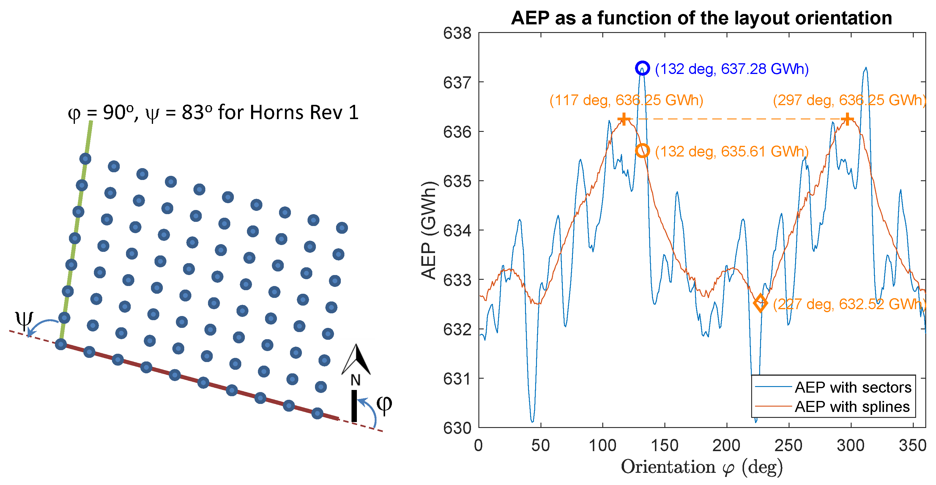
5. Effect of the Number of Wind Rose Sectors on AEP Calculation

5.1. Introduction and State of the Art

Meteorological data obtained in the past are used to estimate the wind conditions during the lifetime of the planned wind farm. If specific site data are not available, researchers may also use other resources for the estimation of time series using global climate reanalysis databases such as ERA5 or MERRA-2. Preferably, the raw time series thus obtained should be used, since any preprocessing or classification will lead the result away from reality. This approach is used in [26] to determine the optimal positioning of wind turbines within a wind farm.
However, it is common in research studies for the estimated data thus obtained to be classified into a set of sectors. In IEC 61400-12-3 [6], a Δ θ = 10 deg is established for the classification of data obtained from meteorological stations. This grouping assumes that wind conditions are identical for all wind directions within that sector. This means that a certain probability distribution, typically a Weibull distribution [19], is associated with all wind directions in the same sector, and that all directions within the sector share the same frequency of occurrence.
It is important to note that this sector-based distinction differs from the directional bin discretization with size δ θ used for AEP calculation in (2). This aspect is addressed by Feng and Shen [27] who compare the obtained values for AEP in HR1 for five different values of δ θ , between 1 deg and 30 deg, concluding that the wind rose should be discretized using 1 deg directional sectors (and wind speed intervals of 1 m/s) in order to achieve reliable and consistent optimization results. The error introduced by a coarse discretization is also discussed in [4].
The common value in research works for the number of the wind rose sectors is 12 [28]. Different values are used in numerous works, as in [29] who conducts a repowering study at Horns Rev 1 and uses 6 deg wind binning, based on data collected over 14 years, in order to estimate the changes in energy output when removing WTs. Kirchner and Porté [30] utilized a wind rose comprising 72 directional sectors (with a 5 deg angular resolution) and 22 discrete wind speed classes (with a 1 m/s resolution) during the operation of a multi-objective optimization of the power output at the Horns Rev I OWF. They also use this sector size as δ θ . Díaz et al. [31] employed two wind roses with 16 and 32 directional sectors, respectively. For each sector, a single predominant wind speed is considered in the estimation of the wind farm’s capacity factor. The study demonstrates that increasing the angular resolution to 32 sectors leads to a reduction in estimation error.
Feng and Shen emphasized in [19] that the number of sectors used in wind direction has a strong effect on the optimized layout, and that using a limited number of sectors (e.g., 12) in the wind rose leads to unrealistically high power outputs. In order to obtain consistent and reliable optimization results, up to 360 sectors or more have to be used. However, they add that this will largely increase the computation cost, which is debatable if the preprocessing is performed prior to the optimization process, and the number of sectors is decoupled from the bin size.
When no time series are available, Gonzalez et al. in [1] propose the transformation of wind rose and the sector-wise Weibull distributions into continuous values. This is performed by applying cubic spline interpolation to derive a continuous wind rose from a discretized one, ensuring that the cumulative probability is preserved within each sector. The same is also applied to the sector-wise distribution of Weibull parameters, ensuring that the mean value of the Weibull distribution parameters are maintained.
In the following, the effect of classifying temporal data into excessively wide sectors is analyzed.

5.2. Method

The IEC standard 61400-12-3:2022 establishes a Δ θ = 10 deg for the collection of historical wind direction data. However, the general practice is to use a sectorized representation of wind conditions with a Δ θ = 30 deg. In [1], a procedure is presented that uses cubic spline interpolation to transform a sectorized distribution (with Δ θ = 30 deg) into a uniform distribution, or at least one with improved resolution, specifically with Δ θ = 1 deg. This is applied to the wind rose in order to obtain a smoothed probability distribution, and to the Weibull parameters, in order to achieve continuous wind conditions.
Among the boundary conditions used in that work is that the mean of the continuous probability density distribution must match the frequency of occurrence in each sector of the wind rose. Similarly, for the Weibull parameters A and k, it is imposed that the mean of the continuous distribution in each sector must coincide with the original Weibull parameter for that sector. However, when using this continuous probability distribution and Weibull parameters with a given turbine to compute the AEP, a mean power output of P a v s e c = 1080.47 MW is obtained using sectorized input data, whereas P a v s p l = 1082.38 MW is obtained using spline-based uniformization. This represents an increase in δ s p l = 0.177 % when using the spline tool.

5.3. Result

Taking this correction into account, the comparison shown in Figure 4 has been produced. The project in C# (Hypothesis.zip) that calculates the data as well as the script in Matlab to represent them (Main_Analyze_Sector_vs_Uniform.m) are provided in [5]. The figure illustrates the AEP estimation for a rhomboidal wind farm with the characteristics of HR1, but allowing for variation in the orientation of the farm φ (which for HR1 is 90 deg with respect to north). The blue curve corresponds to a sectorized distribution with Δ θ = 30 deg, while the orange curve uses spline interpolation to achieve a resolution of Δ θ = 1 deg.
A greater variation can be observed in the estimation of AEP when relying on the sector-wise distribution ( Δ θ = 30 deg), which is not intuitive. Using this sector distribution, if this Δ θ is applied in an algorithm to find the optimal orientation, the study would conclude (see Figure 4) that the best orientation is 132 deg with an AEP = 637.28 GWh. However, using a finer discretization (splines with Δ θ = 1 deg), the estimated AEP decreases to 635.61 GWh, representing a reduction of 0.752%.
Using this finer discretization (splines with Δ θ = 1 deg), the optimal orientation would be 117 deg or 297 deg, with an AEP = 636.25 GWh, which is 0.64 GWh higher than the previously mentioned 635.61 GWh. Compared to the maximum difference of 636.25 GWh–632.52 GWh, this represents an improvement of 17.16%.

5.4. Conclusion and Discussion

Consequently, in the absence of actual historical data, it is highly advisable to transform the sectorized wind data into uniform datasets (or at least into a higher number of sectors), since a representation with few sectors (high Δ θ ) does not accurately reflect the real characteristics of the wind, especially at the boundaries between sectors.
This study analyzes the effect of reducing the size of the sectors ( Δ θ ) used to represent wind conditions. This parameter is often confused with wind direction bin size in deg ( δ θ ), which refers to the angular increment used when discretely calculating an integral over 360 degrees (see Equations (1) and (2)).

6. The Energy Rose: A Novel Representation of Wind Resource Potential

6.1. Introduction

Building on previous studies and the achievements presented in this article, a novel representation of wind resource potential is proposed. A similar motivation is found in [32], where, in order to explore the wind power generation potential of offshore wind farms, the authors consider the Chinese coastline covered with wind turbines of 150 m in diameter arranged in a typical layout. This approach allows them to provide an estimate of the expected energy output at each potential location.
With a more natural approach, a novel representation of wind resource potential is proposed: the energy rose. This unified framework integrates wind rose data (sector-specific occurrence probability) with sector-wise wind speed distribution.

6.2. Method

When analyzing the wind conditions at a site, an accurate calculation requires historical wind data over a sufficiently long period. However, due to the unwieldy nature of this data set, research articles typically use, as input data, a sector-based representation (usually 12 sectors) consisting of three arrays: the probability of wind occurrence in each sector; scale factor of the Weibull distribution (A); and shape factor of the Weibull distribution (k), both corresponding to the Weibull distribution that best fits the wind speed data in each sector.
This sector-based distribution should allow the designer to determine the relative arrangement of the turbines in such a way as to minimize wake losses. To that end, the three data sets are traditionally merged into a single chart, where it is difficult to distinguish the “quality” of the wind in each sector (see Figure 5a corresponding to a site with the wind conditions listed in Table 5).
In this work, we propose combining the three data sets into a one-dimensional representation that provides information on the wind energy in each sector, taking into account both wind intensity and its probability of occurrence. Figure 5b (blue line) shows this representation, which depicts the mean kinetic energy of the wind per second in each sector θ per unit surface area, calculated using the following expression:
K . E . s = u B u 1 2 ρ a i r u 3 fr s wr ( u ) δ u .
where ρ a i r = 1.225 kg/m3 is the air density. In Figure 5b, the red line shows the same representation after being smoothed using cubic spline interpolation, as explained in [1]. This transformation offers a more realistic representation of wind behavior.
However, the value of kinetic energy calculated with (24) is not representative of the energy that a turbine can extract from the wind, since it would need to be multiplied (in addition to the rotor swept area) by the Cp coefficient, which is not constant for different wind speeds and also depends on the turbine model. The expression for the average power captured by a turbine for the sector s is given by
P s a v = u B u P c ( u ) fr s wr ( u ) δ u .
which provides the average energy extracted by the turbine in one second. Representing this value across the different wind directions would yield a one-dimensional curve that provides relevant information about the directions with the highest energy yield, although this value is theoretically dependent on the power curve and, therefore, on the specific turbine.

6.3. Results

Figure 6 shows this value (either sectorized or smoothed) for three different turbines: Vestas V80 2MW, DTU 10 MW, and the averaged virtual turbine of Table 1. Their power curves can be found in [5] (DataTurbines.m). It can be observed that, although the turbine models differ, the representations are very similar and also closely resemble that of Figure 5b). Consequently, the representation shown in Figure 5b) can be used to identify the most productive wind directions. It has the advantages of being one-dimensional—unlike Figure 5a)—and independent of the turbine model used.
The Matlab script (MainEnergyRoses.m) used for these calculations and plots is available in [5].

6.4. Conclusions

A novel representation is proposed that identifies the most and less productive wind directions. It is one-dimensional, unlike the traditional representations with a wind rose with sectors divided into colors representing the speed ranges. It is also independent of the turbine model used.

7. Discussion

There are numerous studies aimed at estimating the energy produced by a wind farm, taking into account the frequency with which the wind blows at different speeds and from various directions. However, there is a clear trend toward remunerating the energy produced based on the electricity market price per MWh, which varies significantly depending on factors such as the time of day and the season of the year. This calls for a shift in the optimization approach, as the profitability of the wind farm will depend not only on the total energy produced, but also on how that production is distributed throughout the day and the year. Some studies along these lines include [33,34,35].
It would be advisable to define new indicators that account for these variations, as in [32], which analyzesd seasonal variations along the coast of China and introduces three indicators to assess the monthly variability of wind conditions.
In addition, the proliferation of photovoltaic panels is inverting the shape of electricity price curves. For example, in sunny countries, summer afternoons—traditionally energy deficient due to the high demand from air conditioning—are becoming energy surplus periods. The emergence of electric vehicle batteries also introduces a factor that must be considered in the near future, as it adds a new player in the supply–demand matching mechanisms during nighttime hours.

8. Conclusions

Many studies on wind farm optimization adopt, without a critical evaluation, a standard AEP calculation formula based on sectorized wind conditions along with a fixed discretization of wind speed and direction. These studies often claim that their optimization algorithms result in increased energy production without considering that the associated estimation and calculation errors of wind conditions may outweigh the supposed improvements.
In this work, these sources of error are analyzed from three different perspectives:
  • The parameters of the Weibull distribution, which are typically derived using purely statistical tools to represent the actual frequency of wind speeds, often lead to significant errors in the estimation of AEP, usually underestimating it. This study proposes using a typical power curve (such as that of the DTU 10 MW reference turbine) to determine the Weibull parameters that best fit the power output derived from historical data.
  • Most studies that conduct a thorough evaluation of AEP across the full wind speed range between uci and uco use a discretization of 1 m/s. This work proposes either using Equation (17) or assessing the error introduced by discretizations of 0.5 m/s and 2 m/s, with the goal of improving accuracy or reducing the CT.
  • Many studies confuse the terms direction bin (related to the discretization used in AEP evaluation) and sector (related to the classification of wind data from historical records). While it is intuitive that a coarser direction binning (larger δ θ ) will introduce greater errors, a coarser sectorization (larger Δ θ ) can also result not only in errors, but in an unrealistic representation of the wind farm’s behavior depending on the relative orientation of its turbines.
In addition, this work provides recommendations for reducing computational time by assuming symmetrical behavior in wind conditions.
Finally, a new representation, polar and one-dimensional, of wind conditions is proposed, which clearly highlights the wind directions that offer the highest energy yield. In this work, it is referred to as the energy rose.

Author Contributions

Conceptualization, A.G.G.-R.; methodology, A.G.G.-R. and J.M.R.-M.; software, A.G.G.-R., J.M.R.-M. and I.R.-R.; validation, A.G.G.-R., J.M.R.-M. and I.R.-R.; formal analysis, A.G.G.-R.; investigation, A.G.G.-R. and J.M.R.-M.; resources, J.M.R.-M.; data curation, J.M.R.-M., I.R.-R. and J.V.M.-D.; writing—original draft preparation, A.G.G.-R. and J.M.R.-M.; writing—review and editing, J.V.M.-D.; visualization, J.M.R.-M. and J.V.M.-D.; supervision, I.R.-R. and J.V.M.-D.; project administration, A.G.G.-R.; funding acquisition, J.M.R.-M. All authors have read and agreed to the published version of the manuscript.

Funding

This work was subsidized by CONCYTEC through the PROCIENCIA Program under the framework of the contest “Scholarships in educational doctorate programs through inter-institutional partnerships”, according to contract PE501090502-2024-PROCIENCIA-BM and the Interinstitutional Alliances Contest for Doctoral Programs corresponding to the UNIVERSIDAD NACIONAL DE INGENIERIA, according to contract PE501084296-2023-PROCIENCIA-BM.

Informed Consent Statement

Not applicable.

Data Availability Statement

The original data presented in the study are openly available in [5].

Conflicts of Interest

The authors declare no conflicts of interest. The funders had no role in the design of the study; in the collection, analyses, or interpretation of data; in the writing of the manuscript; or in the decision to publish the results.

Abbreviations

AEPAnnual Energy Production
OWFOffshore wind farm
WFwind farm
HR1Horns Rev 1
ntnumber of turbines
nsnumber of sectors
ucicut-in speed
ucocut-out speed
fr ( θ , u ) density of probability at wind direction θ and wind speed v
Pcelectric power given by the turbine manufacturer’s power curve
CpPower factor
CTcomputational time
θ wind direction, in deg
ufree stream wind speed in m/s
v t * wind speed in m/s at turbine t taking into account wake effect
fr s wr probability that the wind comes from sector s, given by the wind rose
fr s Wb ( u ) probability that the wind comes from sector s, given by the Windbull distribution
Ascale factor of the Weibull distribution
kshape factor of the Weibull distribution
δ u wind speed bin size in m/s
δ θ wind direction bin size in deg
Δ θ sector size

References

  1. Gonzalez-Rodriguez, A.; Serrano-González, J.; Burgos-Payán, M.; Riquelme-Santos, J. Realistic optimization of parallelogram-shaped offshore wind farms considering continuously distributed wind resources. Energies 2021, 14, 2895. [Google Scholar] [CrossRef]
  2. Herbert-Acero, J.F.; Probst, O.; Réthoré, P.E.; Larsen, G.C.; Castillo-Villar, K.K. A review of methodological approaches for the design and optimization of wind farms. Energies 2014, 7, 6930–7016. [Google Scholar] [CrossRef]
  3. Shakoor, R.; Hassan, M.Y.; Raheem, A.; Wu, Y.K. Wake effect modeling: A review of wind farm layout optimization using Jensen’s model. Renew. Sustain. Energy Rev. 2016, 58, 1048–1059. [Google Scholar] [CrossRef]
  4. Gonzalez-Rodriguez, A.G.; Burgos-Payan, M.; Riquelme-Santos, J.; Serrano-González, J. Reducing computational effort in the calculation of annual energy produced in wind farms. Renew. Sustain. Energy Rev. 2015, 43, 656–665. [Google Scholar] [CrossRef]
  5. González Rodríguez, A.G. Projects in Matlab and C# Regarding the Wind Rose for the Evaluation of AEP. 2025. Available online: https://zenodo.org/records/15470904?preview=1 (accessed on 18 June 2025).
  6. International Standard IEC 61400-12-3:2022; Wind Energy Generation Systems—Part 12-3: Power Performance—Measurement Based Site Calibration. International Electrotechnical Commission: Geneva, Switzerland, 2022.
  7. Serban, A.; Paraschiv, L.S.; Paraschiv, S. Assessment of wind energy potential based on Weibull and Rayleigh distribution models. Energy Rep. 2020, 6, 250–267. [Google Scholar] [CrossRef]
  8. Singh, K.; Bule, L.; Khan, M.G.; Ahmed, M.R. Wind energy resource assessment for Vanuatu with accurate estimation of Weibull parameters. Energy Explor. Exploit. 2019, 37, 1804–1832. [Google Scholar] [CrossRef]
  9. Chaurasiya, P.K.; Ahmed, S.; Warudkar, V. Comparative analysis of Weibull parameters for wind data measured from met-mast and remote sensing techniques. Renew. Energy 2018, 115, 1153–1165. [Google Scholar] [CrossRef]
  10. El-Bshah, A.; Al-Wesabi, F.N.; Al-Kustoban, A.M.; Alamgeer, M.; Nemri, N.; Eltahir, M.M.; Mahgoub, H.; Negm, N. Resource assessment of wind energy potential of Mokha in Yemen with weibull speed. Comput. Mater. Contin. 2021, 69, 1123–1140. [Google Scholar] [CrossRef]
  11. Raichle, B.W.; Carson, W.R. Wind resource assessment of the Southern Appalachian Ridges in the Southeastern United States. Renew. Sustain. Energy Rev. 2009, 13, 1104–1110. [Google Scholar] [CrossRef]
  12. Abbas, G.; Ali, A.; Othman, M.T.B.; Nawaz, M.W.; Rehman, A.U.; Hamam, H. A novel energy pattern factor-based optimized approach for assessing Weibull parameters for wind power applications. Sci. Rep. 2025, 15, 37. [Google Scholar] [CrossRef]
  13. International Standard IEC 61400-12-2:2022; Wind Energy Generation Systems—Part 12–2: Power performance of electricity producing wind turbines based on nacelle anemometry. International Electrotechnical Commission: Geneva, Switzerland, 2022.
  14. Wais, P. A review of Weibull functions in wind sector. Renew. Sustain. Energy Rev. 2017, 70, 1099–1107. [Google Scholar] [CrossRef]
  15. Gonzalez-Rodriguez, A.G.; Roldan-Fernandez, J.M.; Serrano-Gonzalez, J.; Muñoz-Díez, J.V. Gradient Descent Algorithm with Greedy Repositioning Using Power Deficit Aggregation of Wakes to Accelerate the Offshore Wind Farm Layout Optimization Problem in Irregular Concession Areas. Appl. Sci. 2024, 14, 11331. [Google Scholar] [CrossRef]
  16. Troen, I.; Petersen, E.L. European Wind Atlas; Risø National Laboratory: Roskilde, Denmark, 1989. [Google Scholar]
  17. International Standard IEC 61400-12-6:2022; Wind Energy Generation Systems—Part 12–6: Measurement Based Nacelle Transfer Function of Electricity Producing Wind Turbines. International Electrotechnical Commission: Geneva, Switzerland, 2022.
  18. International Standard IEC 61400-12-1:2022; Wind Energy Generation Systems—Part 12-1: Power Performance Measurements of Electricity Producing Wind Turbines. International Electrotechnical Commission: Geneva, Switzerland, 2022.
  19. Feng, J.; Shen, W.Z. Solving the wind farm layout optimization problem using random search algorithm. Renew. Energy 2015, 78, 182–192. [Google Scholar] [CrossRef]
  20. Gonzalez-Rodriguez, A.G.; Serrano-Gonzalez, J.; Burgos-Payan, M.; Riquelme-Santos, J. Multi-objective optimization of a uniformly distributed offshore wind farm considering both economic factors and visual impact. Sustain. Energy Technol. Assess. 2022, 52, 102148. [Google Scholar] [CrossRef]
  21. Ghaisas, N.S.; Archer, C.L. Geometry-based models for studying the effects of wind farm layout. J. Atmos. Ocean. Technol. 2016, 33, 481–501. [Google Scholar] [CrossRef]
  22. Al-Yahyai, S.; Charabi, Y.; Gastli, A. Geometrical Approach for Wind Farm Symmetrical Layout Design Optimization. In Proceedings of the 2015 IEEE 8th GCC Conference & Exhibition, Muscat, Oman, 1–4 February 2015. [Google Scholar]
  23. Neubert, A.; Shah, A.; Schlez, W. Maximum Yield From Symmetrical Wind Farm Layouts. In Proceedings of the 10th Wind Energy Conference-DEWEK, Bremen, Germany, 17–18 November 2010; Volume 98, pp. 1–4. [Google Scholar]
  24. Turner, S.D.; Romero, D.A.; Zhang, P.Y.; Amon, C.H.; Chan, T.C. A new mathematical programming approach to optimize wind farm layouts. Renew. Energy 2014, 63, 674–680. [Google Scholar] [CrossRef]
  25. van der Laan, M.P.; Andersen, S.J.; Réthoré, P.E.; Baungaard, M.; Sørensen, J.N.; Troldborg, N. Faster wind farm AEP calculations with CFD using a generalized wind turbine model. J. Phys. Conf. Ser. 2022, 2265, 022030. [Google Scholar] [CrossRef]
  26. Jaganath, M.M.; Ray, S.; Choudhury, N.B. Optimal placement of wind turbines: A techno-economic analysis using real-time wind speed data and metaheuristic algorithms. Int. J. Energy Water Resour. 2025. [Google Scholar] [CrossRef]
  27. Feng, J.; Shen, W.Z. Modelling wind for wind farm layout optimization using joint distribution of wind speed and wind direction. Energies 2015, 8, 3075–3092. [Google Scholar] [CrossRef]
  28. Feng, J.; Shen, W.Z.; Xu, C. Multi-Objective Random Search Algorithm for Simultaneously Optimizing Wind Farm Layout and Number of Turbines. J. Phys. Conf. Ser. 2016, 753, 032011. [Google Scholar] [CrossRef]
  29. Hou, P.; Enevoldsen, P.; Hu, W.; Chen, C.; Chen, Z. Offshore wind farm repowering optimization. Appl. Energy 2017, 208, 834–844. [Google Scholar] [CrossRef]
  30. Kirchner-Bossi, N.; Porté-Agel, F. Wind farm area shape optimization using newly developed multi-objective evolutionary algorithms. Energies 2021, 14, 4185. [Google Scholar] [CrossRef]
  31. Diaz, G.P.N.; Saulo, A.C.; Otero, A.D. Full wind rose wind farm simulation including wake and terrain effects for energy yield assessment. Energy 2021, 237, 121642. [Google Scholar] [CrossRef]
  32. Deng, X.; Xu, W.; Xu, Y.; Shao, Y.; Wu, X.; Yuan, W.; Qin, Z. Offshore wind power in China: A potential solution to electricity transformation and carbon neutrality. Fundam. Res. 2024, 4, 1206–1215. [Google Scholar] [CrossRef]
  33. Greenberg, D.; Byalsky, M.; Yahalom, A. Valuation of Wind Energy Turbines Using Volatility of Wind and Price. Electronics 2021, 10, 1098. [Google Scholar] [CrossRef]
  34. Alonzo, B.; Concettini, S.; Creti, A.; Drobinski, P.; Tankov, P. Profitability and Revenue Uncertainty of Wind Farms in Western Europe in Present and Future Climate. Energies 2022, 15, 6446. [Google Scholar] [CrossRef]
  35. Khan, M.A.; Iqbal, M.T. Evaluation of Wind Resources and the Effect of Market Price Components on Wind-Farm Income: A Case Study of Ørland in Norway. Energies 2018, 11, 2955. [Google Scholar] [CrossRef]
Figure 1. Error in the estimation of the AEP relative to the value obtained from the time series data, comparing two methods for fitting the Weibull parameters: using MLE through MATLAB R2022b’s wblfit function () and using a parameter sweep based on a typical power curve ().
Energies 18 03402 g001
Figure 2. Error obtained with respect to the mean power production obtained from (17).
Energies 18 03402 g002
Figure 3. OWF tested in the experiments related to symmetry.
Energies 18 03402 g003
Figure 4. On the left, layout of a rhomboid-shape wind farm (WF). On the right, comparison of the estimated AEP as a function of the orientation angle φ of a rhomboid-shape WF for a wind direction bin Δ θ = 30 deg (blue) and Δ θ = 1 deg (orange).
Energies 18 03402 g004
Figure 5. (a) Traditional representation of wind rose and wind speed distributions. (b) Proposed [kinematic] energy rose, both sectorized and uniformized.
Energies 18 03402 g005
Figure 6. Energy roses for three different wind turbines. The energy produced at each sector in MWh is represented in blue. The red curve represents its density.
Energies 18 03402 g006
Table 1. Power curve with the average values for 17 turbines, scaled to 10 MW.
v (m/s)3.04.05.06.07.08.09.010.011.012.013.014.0
P (kW)00203418471595260839285584743790029718
v (m/s)15.016.017.018.019.020.021.022.023.024.025.0
P (kW)992799839994999510,00010,00010,00010,00010,00010,00010,000
Table 2. Weibull parameters, obtained from MLE (wblfit) and with the proposed sweep using a typical Pc.
Sector123456789101112
A M L E 7.967.507.807.568.498.659.0710.029.8910.059.017.58
k M L E 2.001.941.922.082.172.212.232.332.402.532.302.243
A s w 7.507.607.807.708.608.709.8010.709.8010.508.907.50
k s w 1.522.141.741.601.722.621.541.902.662.023.001.60
Table 3. Comparison of errors in P a v h P a v W at each sector for four turbine models, when weibull parameters are obtained using MLE techniques (wblfit from matlab) and the proposed sweep. Positive values means underestimated ones. The final column is the root mean square.
Sector
Turbine123456789101112RMS
Siemens Gamesa SG 3.6-120 MLE−4.70.60.24.10.32.82.75.11.91.50.71.22.73
Siemens Gamesa SG 3.6-120 sweep0.7−0.30.11.00.8−0.72.01.70.03.6−1.41.01.46
Vestas V112/3450 MLE−4.60.60.24.10.42.62.85.11.30.90.51.22.63
Vestas V112/3450 sweep0.2−0.00.00.70.3−0.31.11.1−0.11.9−0.60.40.77
Vestas V164-8.0 MLE−10.41.60.98.51.95.76.911.40.4−0.5−0.12.25.80
Vestas V164-8.0 sweep−1.20.6−0.2−1.4−1.31.4−2.5−2.4−0.5−5.32.2−2.02.17
DTU Reference 10 MW MLE−13.72.40.612.41.56.89.315.41.00.40.73.47.81
DTU Reference 10 MW sweep−1.10.8−0.50.9−0.90.10.81.0−1.5−1.01.1−0.70.93
Table 4. Inaccuracy in the calculation of AEP when imposing point symmetry.
Offshore Wind FarmAEP (GWh) from (3)AEP (GWh) from (22)Deviation
Anholt1716.13701715.99200.0085%
Donghai Bridge II283.5456283.54610.0002%
East Anglia3049.18243049.24540.0021%
Galloper966.5156966.53020.0015%
Greater Gabbard1353.69651353.64010.0042%
Gwynt y Mor796.8648796.85610.0011%
Hohe See2249.60752249.56820.0017%
Horns Rev1633.7517633.75170.0000%
Horns Rev21071.81951071.81950.0000%
Hornsea 15333.86645333.77260.0018%
Hornsea 25617.59845617.60350.0001%
Kriegers Flak740.6054740.59050.0020%
Lillgrund207.7917207.77730.0069%
London Array1972.77691972.78090.0002%
Nysted442.8121442.81210.0000%
Rampion1175.34501175.35660.0010%
Saint Nazaire1320.06451320.05010.0011%
Triton Knoll2844.10552843.91490.0067%
Table 5. Probability, scale factor, and shape factor for the site under test.
Sector123456789101112
fr wr (%)7.424.075.137.828.336.3210.9010.2312.1210.0311.705.93
A8.719.369.2910.2710.8910.4910.9411.239.9311.949.1710.31
K2.082.222.412.372.512.752.612.512.333.352.582.01
Disclaimer/Publisher’s Note: The statements, opinions and data contained in all publications are solely those of the individual author(s) and contributor(s) and not of MDPI and/or the editor(s). MDPI and/or the editor(s) disclaim responsibility for any injury to people or property resulting from any ideas, methods, instructions or products referred to in the content.

