Achieving Power-Noise Balance in Wind Farms by Fine-Tuning the Layout with Reinforcement Learning

Abstract

Wind farms situated in proximity to residential areas present environmental challenges, primarily due to noise emissions. Rectangular and parallelogram layouts are commonly employed in current wind farm designs owing to their simplicity and visual appeal. However, such configurations often experience significant power loss under certain wind directions because of intense wake interactions. This paper proposes a layout fine-tuning strategy for low-noise wind farm design. Within a reinforcement learning framework integrated with an engineering wake model and a noise propagation model, the positions of two turbines (controlled by two variables) are optimized. The noise propagation model was validated for idealized long-range sound propagation over flat terrain with acoustically soft surfaces. A case study was conducted on a 12-turbine wind farm located on a flat plain in China, with a noise threshold of 45 dB(A) used to assess the noise impact area. Optimization results demonstrate that the proposed method achieves a balance between power output and noise reduction compared to the original regular layout: Annual Energy Production (AEP) increased slightly by 0.16%, while the noise impact area was reduced by 6.0%. Although these improvements appear modest, the potential of the proposed methodology warrants further investigation.

1. Introduction

As an important source of clean and renewable energy, wind power has attracted sustained attention and undergone significant development throughout this century, playing a key role in mitigating the climate crisis associated with global warming while delivering numerous positive impacts. However, in recent years, the depletion of land-based wind resources in high-wind-speed regions has led to the planning and construction of wind farms increasingly closer to residential areas [1]. Concurrently, the growing size of modern wind turbine (WT) rotors has resulted in increasingly significant noise levels during operation [2,3], disturbing the daily lives of nearby residents. To effectively mitigate these negative impacts, it is essential to carefully select suitable WT installation sites and optimize wind farm layout planning [4].

Wind farm layout optimization (WFLO) is widely regarded as one of the most important and challenging research topics in wind energy engineering [5,6,7]. A well-designed layout can significantly reduce negative wake effects caused by upstream WTs—such as velocity deficits and increased turbulence intensity—thereby improving the economic performance of wind farms and reducing operational and maintenance costs. Studies indicate that wake losses within wind farms can reach up to 22% [8,9,10]. Wake recovery is primarily driven by turbulent mixing, which entrains higher-momentum air from the surrounding flow. This process stems from strong shear between the decelerated wake and the free stream, generating energetic vortex structures. However, accurately modeling these phenomena remains challenging due to the limitations of Reynolds-Averaged Navier–Stokes (RANS) models in capturing anisotropic turbulence, while high-fidelity Large Eddy Simulation (LES) methods remain computationally prohibitive for large-scale applications.

At present, wind farm layouts mostly adopt rectangular or parallelogram shapes, which offer simpler design rules and fewer control parameters, and they retain flexibility for further improvement [11,12]. For the foreseeable future, these classical wind farm layouts will continue to be used as the mainstream approach. However, in regularly shaped wind farms, under certain wind directions, several turbines may align almost along the same line with narrow spacing. Under the corresponding wind directions, wakes from upstream WTs propagate downstream, impacting rear turbines and their wakes, leading to intense multiple-wake interactions and serious wake losses, which result in severe power output reductions. Wind farms are highly sensitive to wind directions, and power generation exhibits sudden and unsteady fluctuations with changes in wind directions [11], which is unfavorable for stable grid connection. Unfortunately, this issue is inherent to the layout definition, and no effective method currently exists to address it through layout arrangement. In academic research, 0/1 chessboard layouts are predominant, as they can fully consider wind resource characteristics and achieve high power generation. It has been found that irregular wind farm layouts yield an overall increase of 0.66 % in power output due to reduced wake losses, and the power output is less sensitive to fluctuations in wind direction [13]. On the other hand, such chaotic layouts often lack aesthetic appeal and result in extremely complex cable connections, which can complicate the operation and management of WTs and incur additional costs [14,15]. Consequently, they are rarely applied in practical engineering design.

In recent years, researchers have increasingly sought to balance power generation and noise concerns in wind farm layout design. Nyborg [16] introduced a method for optimizing wind farm noise constraints by adjusting the operational modes of individual WTs, incorporating sound propagation modules within the TopFarm [17] and PyWake frameworks [18]. Wu et al. [19] optimized wind farm layouts by treating minimum noise as a primary objective while accounting for wake effects and mandatory spacing constraints between turbines. They compared basic and enhanced particle swarm optimization algorithms to improve computational efficiency. Further studies have shown that using different WT types—which vary in noise emission levels—can influence optimal turbine positioning [20]. Mittal and Mitra [21] employed established wake and acoustic models to determine the ideal number and placement of WTs, navigating competing objectives such as noise control, power output, and energy cost. Nevertheless, WFLO remains challenging due to the high dimensionality of variables, numerous constraints, and the multimodal nature of the design space. In response, novel techniques and hybrid approaches have been developed to address these complexities [22,23,24]. Previous studies also highlight that as the number of turbines increases, along with complex wake interactions and diverse wind conditions, substantial computational resources are required during iterative layout processes for estimating energy production and conducting noise assessments.

The recent development of the machine learning (ML) methods has attracted significant interest among researchers in the wind energy area. Some studies have developed data-driven WT wake models by inputting high-precision training data and using these efficient machine learning models to optimize wind farm layout [25]. Yang et al. [26] presented a data-driven wind farm layout optimization framework that uses an artificial neural network (ANN) wake model, the ANN models are trained to ensure high prediction accuracy, with less than 2% error compared to CFD simulations. Luo et al. [27] built a data-driven wake model and employed an objective function that maximizes power output; the optimized wind farm layout yields over 210 kW more total power output than the baseline.

As an important branch of ML, reinforcement learning (RL) has gained significant attention and continuous exploration in recent years due to its high efficiency and short time consumption in solving optimization problems. RL has also been gradually applied to wind farm layout optimization. Li [28] applied a policy gradient RL algorithm in which a deep convolutional neural network (CNN) is designed to process high-dimensional states and generate policy and value estimations. The RL was compared with the traditional genetic algorithm (GA) and showed promising results for the WFLO problem. Yu and Lu [29] developed an RL-based multi-objective differential evolution (RLMODE) algorithm to address the complexity of the WFLO problem. The performance of the RLMODE was tested in two wind scenarios, it was observed that the total power generated by the solution from the RLMODE algorithm was larger compared to other optimization methods. Using an adaptive evolutionary algorithm with Monte Carlo Tree Search RL, Bai et al. [30] constructed an RL algorithm to achieve an optimal layout. The algorithm was applied to a recently approved wind farm in New Jersey and showed better performance against benchmark algorithms. Recently, Yu and Zhang [31] proposed a teaching-learning-based optimization algorithm with RL, the superiority of the improved algorithm over others and its effectiveness in addressing wind farm layout problems were demonstrated by experimental results.

It has been proven that ML and RL offer advantages in solving wind farm design problems, and there is still great potential to further develop these methods to enhance their adaptability. The primary distinction between previous studies and our work lies in the research focus. While earlier efforts have primarily applied ML to address wind farm wake modeling and layout optimization driven solely by wake losses, our study extends this application by incorporating both wake effects and noise annoyance in the wind farm layout design process. A key question arises: can an RL-based optimization framework improve power generation while simultaneously mitigating acoustic impact in nearby residential areas?

The main contribution of this study is the development of a fine-tuning layout framework based on deep RL. The framework employs a deep Q-learning agent equipped with a fully-connected neural network utilizing ReLU activation functions and a learning rate of 0.002. It preserves the fundamental structure of the original regular wind farm layout while achieving an optimal balance between power generation efficiency and noise reduction for nearby residential areas. During the layout design phase of low-speed wind farms on flat terrain, the location fine-tuning strategy may provide an approach to modify the local positions of a few turbines, which is closer to engineering practice.

The remainder of the paper is organized as follows. Section 2 introduces the basic principles of wind farm power prediction and noise modeling. Section 3 details the fine-tuning layout strategy and demonstrates the layout optimization framework and corresponding formulation. Section 4 proposes a machine learning model based on a deep Q learning algorithm to obtain an optimal layout considering power yield and noise influence area. Section 5 presents a case study of a wind farm and the prepared data (including layout, power, and noise), along with the layout optimization results of the wind farm fine-tuning optimization, although real-world validation or comparative methods are not included. Finally, Section 6 concludes the study and points out some limitations.

2. Wind Farm Power and Noise

As a classical optimization problem, WFLO involves three aspects of information: wind farm planning region (area, shape), wind resources (wind rose diagram), and WT arrangement rule (regular or irregular). Generally, the standard framework of WFLO can be divided into several modules, such as wind farm layout adjustment, performance evaluation, and optimization algorithms [14,15]. During optimization, the planning region and wind resource remain unchanged, while the WT locations within the planning region are upgraded under an optimization algorithm. Once the wind farm layout changes, the energy production performance under wind resources is evaluated, which determines the next movement of WT locations. The following sections describe the theoretical principles of power generation prediction (based on wake simulation) and noise assessment for wind farms.

2.1. Power Production Calculation

Power production is the primary objective in wind farm development. To accurately predict the annual energy production (AEP) of a wind farm, it is necessary to obtain each turbine’s power yield under various free-stream inflow conditions throughout a year. Due to the wake loss effects, downstream turbines always operate at reduced power levels. Using analytical wake models such as the Jensen model, Frandsen model and Gaussian model, the inflow velocity at the rotor-swept disc of downstream WTs can be evaluated. The power production of each turbine is then obtained according to their power curves. As a consequence, the AEP (in kWh) of the entire wind farm can be estimated.

$$\mathrm{A}\mathrm{E}\mathrm{P}=8760\times {\sum }_{n=1}^{N_{wt}}{\sum }_{s=0}^{360}{\sum }_{o=1}^{U_{max}}{F}_{req}\left(u_o, d_s\right)\times P_{wr}\left(u_o, d_s\right)$$

(1)

where 8760 is the number of hours in one year. The subscripts o and s denote discrete summation over wind speed (u), and direction (d), respectively. The entire range of wind speed (3–25 m/s) and wind direction (0–360°) is divided into adjacent discrete bins. N_wt and U_max are the total number of turbines in a wind farm and the maximum number of wind speed bins, respectively. The frequency of occurrence of wind at different wind directions and speeds is presented as a probability mass function, combined with the period of various wind conditions in a year.

Since existing wake models cannot fully reproduce the real flow field within the wind farm, energy prediction entails notable errors. Furthermore, the choice of bin sizes for wind speed and direction effects model sensitivity [32].

2.2. Noise Evaluation Model

Wind farm noise evaluation is a complex issue, often covering a domain much larger than the wind farm itself. Instead of simulating a noise map everywhere in a wide domain, an alternative approach is to focus on multiple receivers and sum up the noise from each WT propagating to these receivers. The noise at the receivers originating from turbine i can be obtained by:

$$L_p^i\left(f\right)=L_w\left(f\right)-10{\mathrm{l}\mathrm{o}\mathrm{g}}_{10}4\pi D^2-\alpha D+∆L$$

(2)

where L_w (f) is the Sound Pressure Level (SPL) of the noise source at frequency f. The term of 10log₁₀ 4πD², αD and ∆L represent geometric attenuation, atmospheric absorption, and relative sound pressure level, respective. D is the distance between the noise source (WTs) and the sound receptors (e.g., human habitats). α is the atmospheric absorption coefficient. In this study, a relative humidity of 70% and temperature of 10 °C are assumed, yielding an α value of 0.005 dB/m. Geometric attenuation corresponds to the spherical spreading of sound waves from a point source. Any deviation from ideal conditions can be represented by ∆L such as ground reflection, atmospheric refraction, atmospheric turbulence, irregular terrain, and noise barriers. Under the assumed ideal conditions, only ground reflection is considered, while other effects such as terrain irregularities, atmospheric refraction, and turbulence are excluded.

∆L is a critical value in wind farm noise evaluation. Here, the wide-angle propagation equations (WAPE) method is employed to simulate long-distance sound propagation. The solution of each WAPE simulation yields a steady solution at each frequency [33]. Several computational approaches exist to solve these equations, among them, the Crank-Nicolson Parabolic Equations (CNPE) method is an efficient choice. The CNPE method can be simplified into a two-dimensional (2D) form based on an axisymmetric approximation [34]. The parabolic equation is solved using the CNPE method in the x-direction and central finite differences in the z-direction, the computational domain is illustrated in Figure 1. As shown, the WT noise source is located at x = 0 at a certain hub height. The noise source is redistributed along the z-axis and propagates along the x-axis. From iteration n to n + 1, the source P(x) is updated to P(x + dx) using the CNPE method. Thus, at any receiver point within the domain, the propagation loss ∆L is recorded.

At each sound receiver location, the total noise spectrum is obtained by superimposing the noise levels from n WTs at receiver r:

$$L_r\left(f\right)=10{\log }_{10}\left(\sum _{i=1}^n{L}_p^i\left(f\right)\right)$$

(3)

The CNPE method is employed to evaluate the noise influence in the resident zone, and the A-weighted SPL from every WT at each receiver is obtained. The reliability and accuracy of the PE method have been validated in previous studies [35,36,37].

3. Wind Farm Layout Optimization

3.1. Wind Turbine Location Fine-Tuning

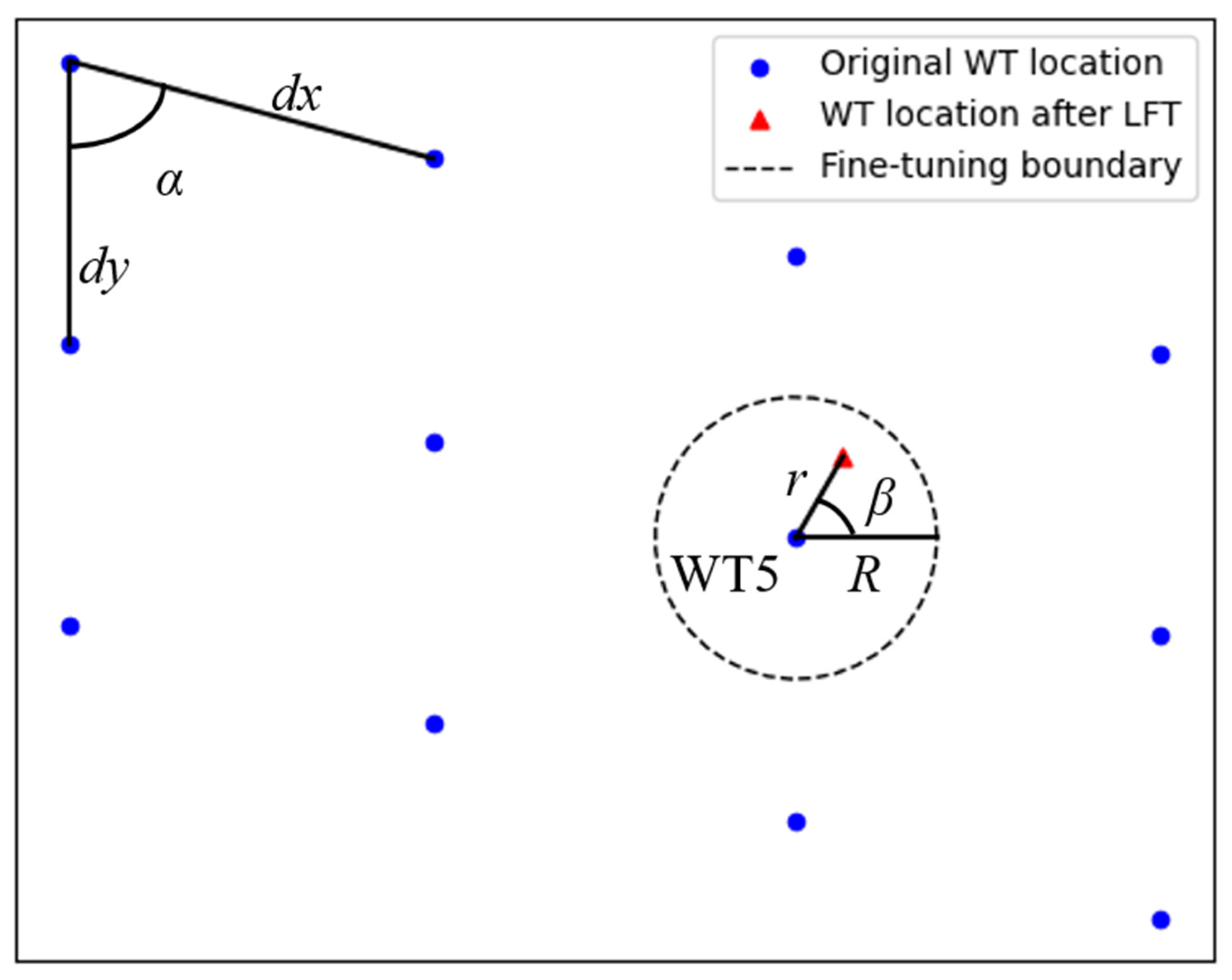
In engineering wind farm programs, the parallelogram layout (a rectangular is a special parallelogram with a 90° angle) is the most widely used type, especially on flat land and offshore regions. The reasons include simplicity, regular and aesthetic shape, ease of installation, cabling and maintenance, and fewer design variables, such as down-wind spacing dx, cross-wind spacing dy, and tilt angle α, as demonstrated in Figure 2. On the other hand, since the shape of the layout is regular, the power loss can be significant due to multiple wakes interference under specific wind directions.

To address the shortcomings of the traditional regular wind farm layouts, a wind turbine location fine-tuning (LFT) strategy is proposed in this study. The strategy is capable of reducing wake loss to some extent while maintaining a layout shape similar to a parallelogram. As illustrated in Figure 2, based on the original parallelogram layout (blue dots), a circular boundary (black dash lines) is generated with a given maximal radius R. Then, two geometrical parameters (radius r and angle β) control the allowed position of WT7 (red triangle). The resulting wind farm layout resembles a parallelogram, but the rows and columns are not perfectly aligned, reducing wake overlap in some wind directions. This decreases wake loss and increases power generation.

To demonstrate the effectiveness of the LFT strategy, it is applied to WT5 in a wind farm (Figure 2) with 3 × 4 arrays of 6.45 MW WTs. The rotor diameter D is 130 m, other properties and wake modeling details are provided in Section 5.1. For the original layout, dx = 8D, dy = 6D, and α = 75°. For WT5 under the LFT strategy, R = 3D, r = 2D and β = 30°. These values were chosen for illustrative purposes to demonstrate the framework application, and R was determined through empirical tests. They are not intended as universal or optimal values. The framework allows all parameters to be adjusted based on specific practical requirements and priorities, such as energy production targets, noise constraints, site conditions, or technological configurations.

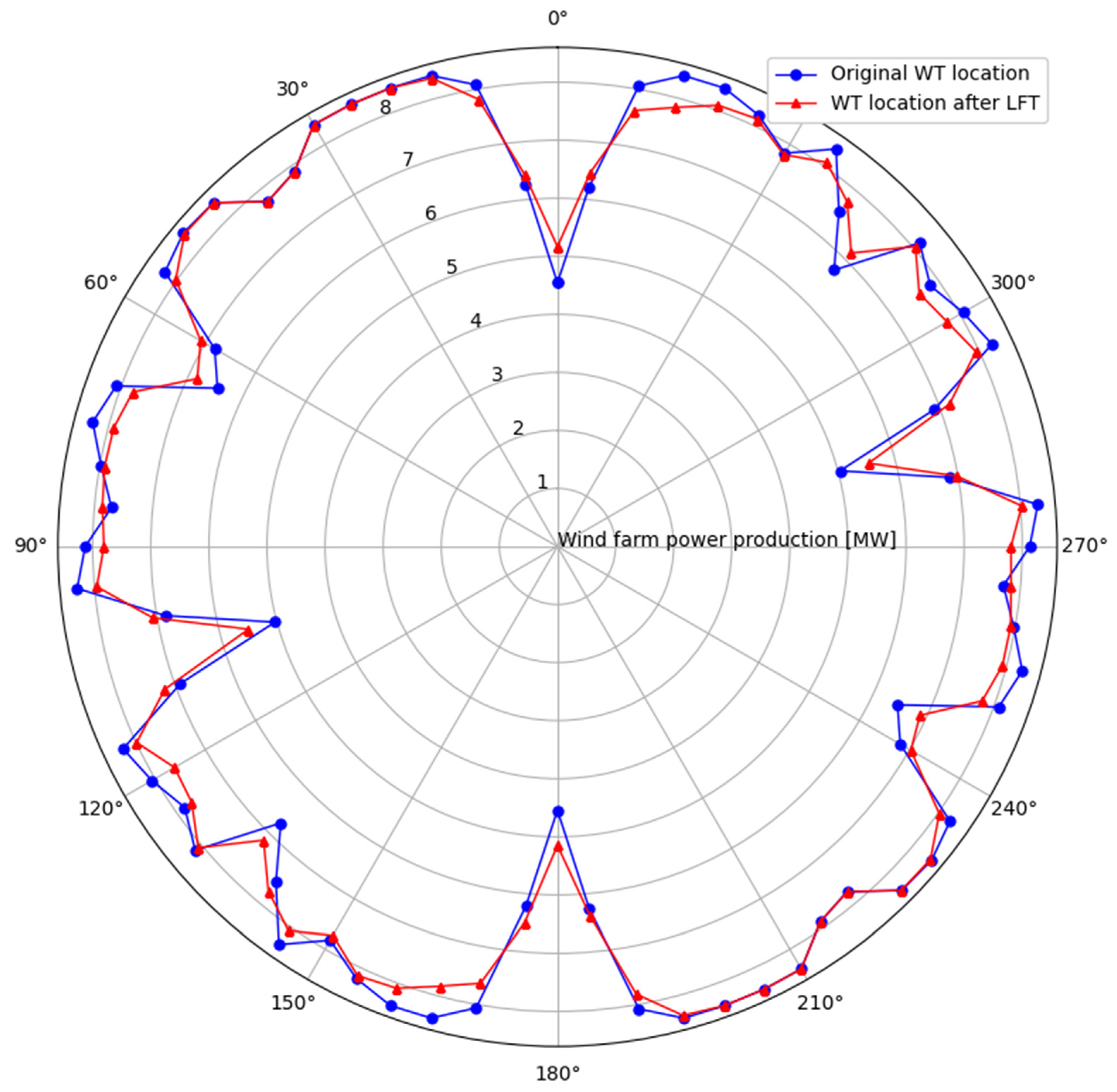
At a wind speed of 6 m/s, the power production curves of the wind farm before and after LFT are displayed in Figure 3. Clearly, under wind directions of 0° and 180°, the output after LFT shows a significant improvement of 13.72%. As illustrated in Figure 4, the wind speed distribution contours at hub height under a 180° wind direction indicate that after LFT, WT5 moves out of the aligned full wake, increasing the wind rate at its hub center from 3.61 m/s to 5.84 m/s. This leads to a remarkable enhancement in the generation efficiency of WT5 with similar effects observable in other wind directions.

Subsequently, the LFT strategy is employed to find an optimal layout that achieves a power-noise balance. The workflow details are described in the next sentence.

3.2. Problem Formula

The solution to the WFLO problem relies on the target functions, constraints, and variable bound. In previous investigations, maximizing AEP and limiting noise level at given points (representing human habitats) were treated as the goal function and constraint, respectively [23,24]. In this study, for a wind farm layout near a resident zone, the objective function and constraint are set as follows.

$$\begin{array}{c}\mathrm{m}\mathrm{a}\mathrm{x}\mathrm{i}\mathrm{m}\mathrm{i}\mathrm{z}\mathrm{e}\hspace{1em}{G}_{PN}={{\lambda }_{1}G}_{AEP}+{{\lambda }_{2}G}_{ANI}={\lambda }_1{\displaystyle \frac{{\mathrm{A}\mathrm{E}\mathrm{P}}_n-{\mathrm{A}\mathrm{E}\mathrm{P}}_0}{{\mathrm{A}\mathrm{E}\mathrm{P}}_0}}-{\lambda }_2{\mathrm{A}\mathrm{N}\mathrm{I}}_n\\ \mathrm{w}\mathrm{i}\mathrm{t}\mathrm{h} \mathrm{r}\mathrm{e}\mathrm{s}\mathrm{p}\mathrm{e}\mathrm{c}\mathrm{t} \mathrm{t}\mathrm{o} mi, i=1, 2, \dots , N_{wt}\\ \mathrm{S}\mathrm{u}\mathrm{b}\mathrm{j}\mathrm{e}\mathrm{c}\mathrm{t} \mathrm{t}\mathrm{o} {\left(x_n-x_0\right)}^2+{\left(y_n-y_0\right)}^2<R^2\end{array}$$

(4)

The gains in AEP improvement G_AEP and noise area reduction G_ANI, weighted by ${\lambda }_1$ and ${\lambda }_2$, respectively, are integrated into a single objective function G_PN. The weights ${\lambda }_1$ and ${\lambda }_2$ were chosen arbitrarily to reflect a sample trade-off between energy output and noise reduction. In real-world applications, these values can be calibrated based on stakeholder preferences, regulatory guidelines, or performance objectives. Here, they are set to 0.8 and 0.2, respectively. This function evaluates the comprehensive performance in power production and noise influence of the wind farm layout. The subscriptions 0 and n denote the original layout and the layout after LFT, respectively. The ratio of $({\mathrm{A}\mathrm{E}\mathrm{P}}_n-{\mathrm{A}\mathrm{E}\mathrm{P}}_0)/{\mathrm{A}\mathrm{E}\mathrm{P}}_0$ represents the AEP increases due to LFT. The term ANI denotes the noise influence area, where the SPL of the receivers exceeds the threshold of the local noise regulations. According to relevant noise regulations, the resident area belongs to the first-level noise standard area, with limits of 55 dB(A) during the day and 45 dB(A) at night [38]. The area with noise level exceeding 45 dB(A) is defined as the noise influence (unacceptable) area in this study.

For the WFLO problem, x and y are the continuous location coordinates of each turbine. The turbine location is constrained to a circle of radius R.

As noted in Section 2.1, AEP calculation involves hundreds of wind conditions, and corresponding wake and noise propagation simulations require substantial computational effort, especially for large wind farms with numerous WTs. The final solution to the WFLO problem typically requires a large deal of iterations, making performance evaluation time-consuming. Given that data-driven models offer powerful prediction and generality capabilities, we propose a data-driven model based on RL technology to save iterative time and cost while achieving a subtle balance between AEP and noise. Details of the RL model are introduced in Section 4.

4. RL-Based WFLO Model

4.1. Deep Q Learning Algorithm

RL is a representative ML technique where agents interact with the environment through a trial-and-error approach and learn an optimal behavior based on the rewards from past interactions. RL techniques can be divided into model-free and model-based categories. Compared to the model-based method, model-free RL is highly flexible and can be more easily coordinated with optimization algorithms [39]. Q-learning, a popular model-free RL technique, evaluates the value of an action $a$ in a state based on the current Q-value and reward. It has a simple structure and does not require explicit prior modeling of the environment. In many RL algorithms, learning updates (e.g., gradient steps) can be performed during an iteration without requiring the episode/task to complete.

In the Q-learning algorithm, the Q-table is the most important element. It determines which action an agent should perform. The agent takes the action and obtains a reward to update the Q-table. The value for each state-action pair in the Q-table is adjusted as follows:

$$Q_{t+1}\left(s_t,a_t\right)=Q_t\left(s_t,a_t\right)+\alpha \left[r_{t+1}+\gamma \underset{a_{t+1}}{max} Q_t\left(s_{t+1},a_t\right)-Q_t\left(s_t,a_t\right)\right]$$

(5)

where $a_t$ is the action the agent can perform, s_t is the state of the agent, Q_t+1(s_t, a_t) is the updated Q-value estimate, the learning rate α and the discount factor γ are parameters between 0 and 1.

These three variables form a two-dimensional Q-table essential for guiding an agent’s decisions in the Q-learning algorithm. The Q-table maps the relationship between states and actions, helping the agent choose the best action for each state. When the state and action spaces are extremely large, traditional Q-learning method may fail since most states are seldom visited, and lookup table storage becomes intractable.

However, as the number of state-action pairs increases, the size of the Q table increases correspondingly. As a result, Q-learning suffers from the curse of dimensionality. To overcome this problem, function approximation is used to approximate the Q function based on statistical regression. Function approximators can be linear models, decision trees, or neural networks in Q-learning with parameter θ. The update rule in Equation (5) is rewritten as:

$${\theta }_t=\mathrm{a}\mathrm{r}\mathrm{g} \underset{\theta }{\min }\mathcal{L}\left(Q\left(S_t,A_t;\theta \right),R_t+\gamma Q\left(S_{t+1},A_{t+1};\theta \right)\right)$$

(6)

where $\mathcal{L}$ represents the loss function, e.g., mean squared error (MSE). The loss is calculated by taking the squared difference between the predicted value and the target value. The optimization problem can be solved by collecting batch samples, constructing the fitted Q iteration.

However, Q-learning is known to be unstable or even divergent when using a non-linear function approximator such as a neural network to represent the Q-value function. With advances in training deep neural networks (DNN), deep Q-networks (DQN) addressed this issue and ignited the research in deep reinforcement learning [40]. The learning agent keeps a dedicated DQN that accepts the current state as an input and outputs value functions for each action in the given state. In this study, DQN is utilized to build the fine-tuning optimization framework.

4.2. DQN-Based WFLO Framework

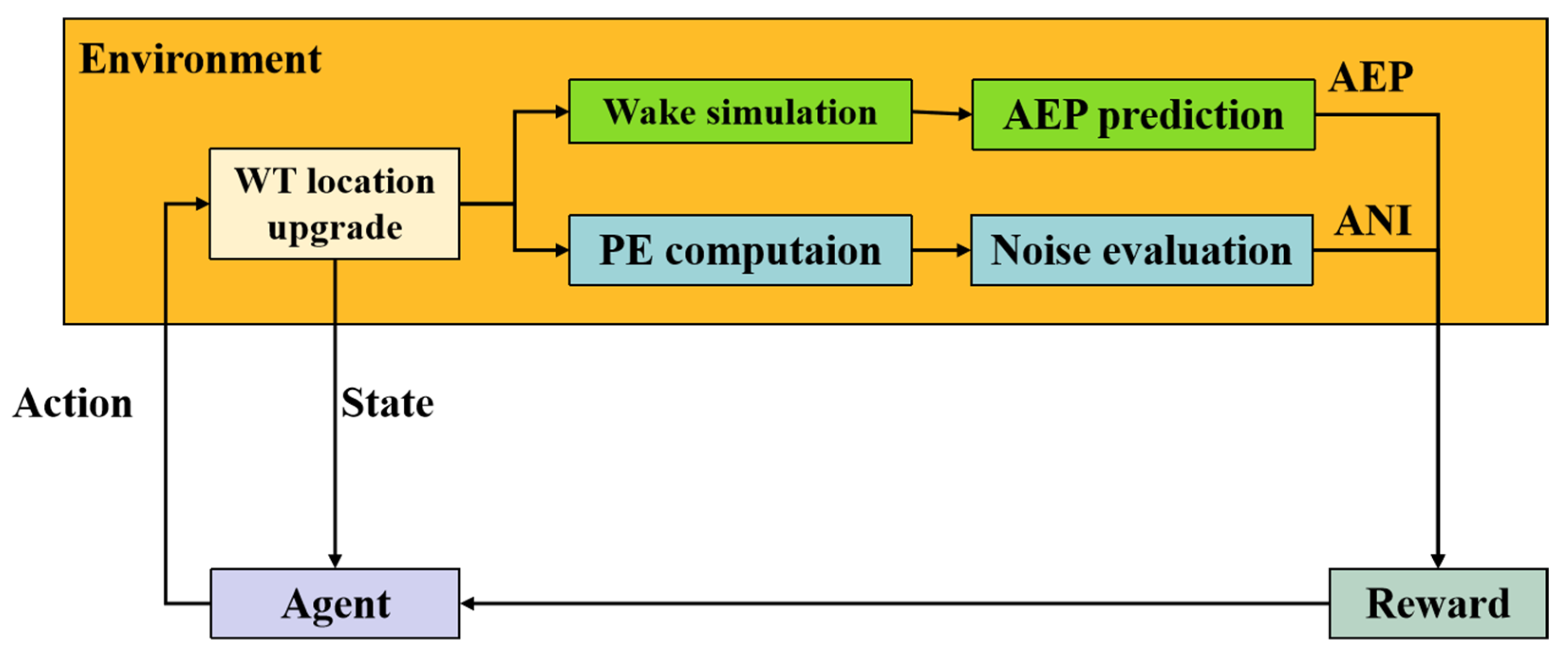
The learning agent generates an action aimed at maximizing cumulative reward by interacting with the environment. For this fine-tuning layout problem, as displayed in Figure 5, the wind farm layout generation, wake simulation, and noise evaluation constitute the environment of the DQN framework. The FLOw Redirection and Induction in Steady State (FLORIS) package, which is used for wind farm wake simulation. The Curl wake model [41], as a kind of Gaussian wake model with considering the yawed inflow effect, and velocity square sum superposition model are adopted, AEP is calculated based on local wind resource data. The PE model described in Section 2.2 is used for noise evaluation. It was validated with the NORD2000 commercial model over flat grass terrain with an acoustically soft surface [42].

In the fine-tuning DQN framework, the three critical RL variables, the state, action and reward are defined as follows:

• State: The state s means the current location (r_j, β_j) (j = 1, 2, …, k) of k WTs under fine-tuning. The state is upgraded by a new action. To improve efficiency, the continuous region is discretized, the step intervals Δr and Δβ are set to 0.2D and 10°, respectively. These values were determined through empirical tests and calibrated against neighboring resolutions (Δr: 0.1D, 0.3D and 0.4D, Δβ: 5° and 15°). These resolution values were chosen based on an initial parameter sensitivity analysis. The guiding principle was to balance computational efficiency and result accuracy. The state is the WT location at the current step.
• Action: The action space encompasses the total available fine-tuning region, with each point being a potential WT location. For the fine-tuning region of k turbines, the action a = (±Δr_j, ±Δβ_j) controls the movement of the turbines. The predefined fine-tuning circle sets the maximum displacement limit. The parameterization is defined by 8 variables (a radius step ±Δr and an angle step ±Δβ for two turbines).
• Reward: The value of GPN of a given wind farm layout represents the reward. Based on the current state and the original layout, the entire wind farm layout (x_i, y_i) (i = 1, 2, …, N) is created. Wake simulations and PE computations are then conducted to obtain total AEP generation and the noise influence area. Finally, rewards are calculated by combining the AEP improvement and noise area reduction.

5. Simulation Study

5.1. Wind Farm Description

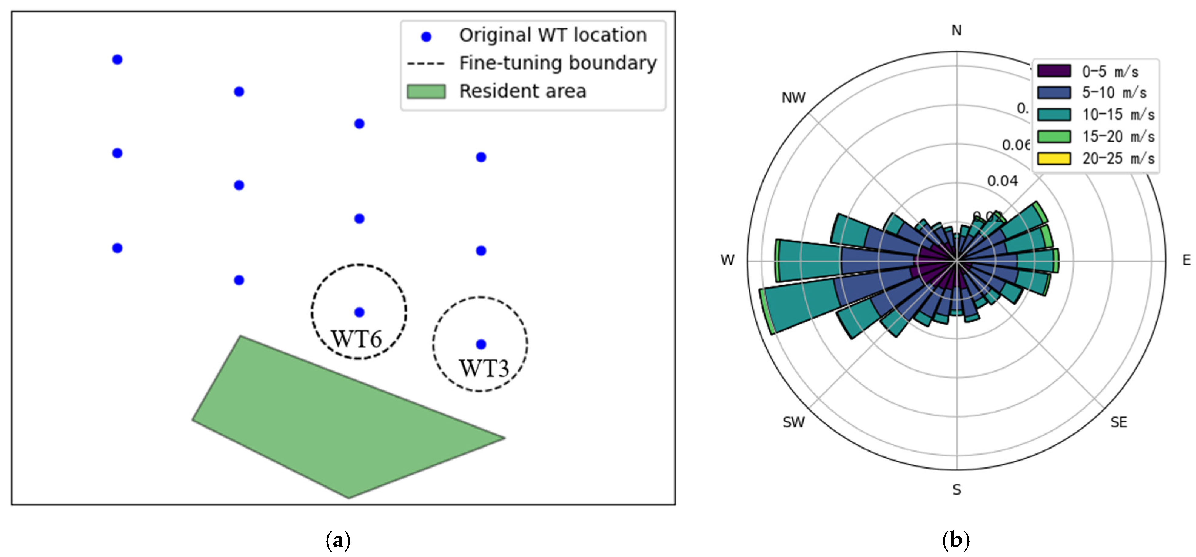
To exhibit the workflow of WT location fine-tuning optimization, a wind farm containing 12 WTs was selected as a case study, as shown in Figure 6. The wind farm is located on flat grassland in China, with an irregular quadrangle in the southeast corner representing a noise-sensitive resident region. According to the design requirements, the locations of neighboring WTs need adjustment to reduce noise influence below a certain level. Based on the original layout, the two nearest turbines (WT3 and WT6) in the lower-right corner are selected for the fine-tuning within a circular region of diameter R. Note that the maximum value of R must be limited to prevent collisions between turbines, the fine-tuning boundaries of the two turbines should maintain a safety distance and avoid overlapping with other turbines.

The turbines have a rated wind power of 6.45 MW at a wind speed of 11 m/s. The rotor diameter D is 130 m with a hub height of 90 m. The cut-in and cut-out speeds are 3 m/s and 25 m/s, respectively. The power coefficient C_p and the thrust coefficient C_t curves are plotted in Figure 7a. The A-weighted SPL of the noise source at rated wind speed, computed with a semi-empirical WT noise model [43], is displayed in Figure 7b. This noise source spectrum serves as input for WT noise propagation modeling.

5.2. Noise Propagation Simulation

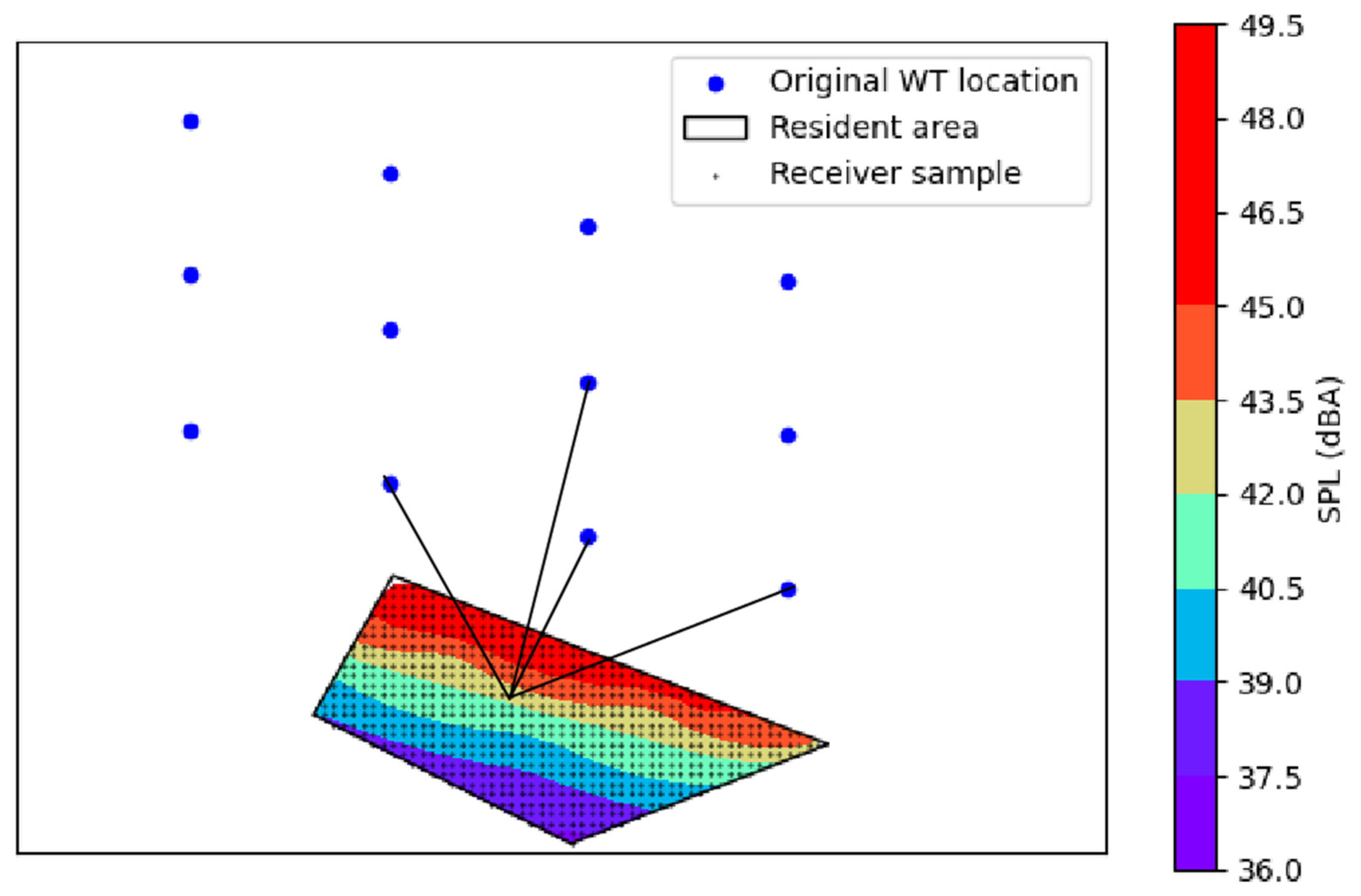
The received noise at 1.5 m height above ground is obtained, and a noise map is generated; the spatial resolution of the noise map depends on the density of selected receiver points. As observed in Figure 8, the residential region in the upper margin has a relatively high SPL exceeding the regulation limit of 45 dB(A) [38]. The proportion of the noise influence area in the entire region is approximately 15.81%. As mentioned, the SPL in the residential region is the sum of contributions from selected WTs. The dominant contribution comes from the nearest WTs. Since SPL mainly depends on the distance between the noise source and the receivers, the two turbines (WT3 and WT6) are targeted for fine-tuning. Geometric modification is identified as the main factor influencing sound propagation. Under the LFT strategy, the noise influence area will vary to some extent once the turbine locations are modified.

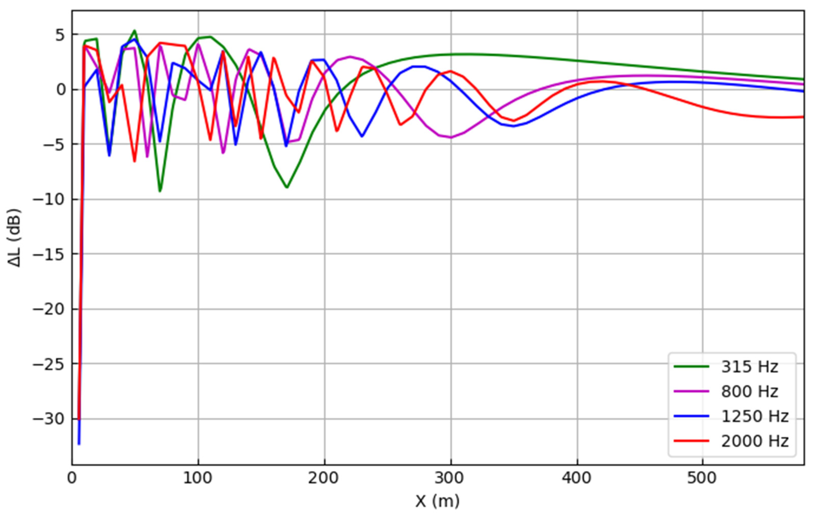
For each receiver in the residential region, the sound level in the 1/3 octave band varied with increasing sound propagation distance from a WT. The relative sound pressure level (ΔL) at four typical frequencies (315 Hz, 800 Hz, 1250 Hz and 2000 Hz) is plotted in Figure 9. At each individual frequency, ΔL generally decreases moderately with distance, though several sudden fluctuations occur within 400 m.

5.3. Building the DQN Agent

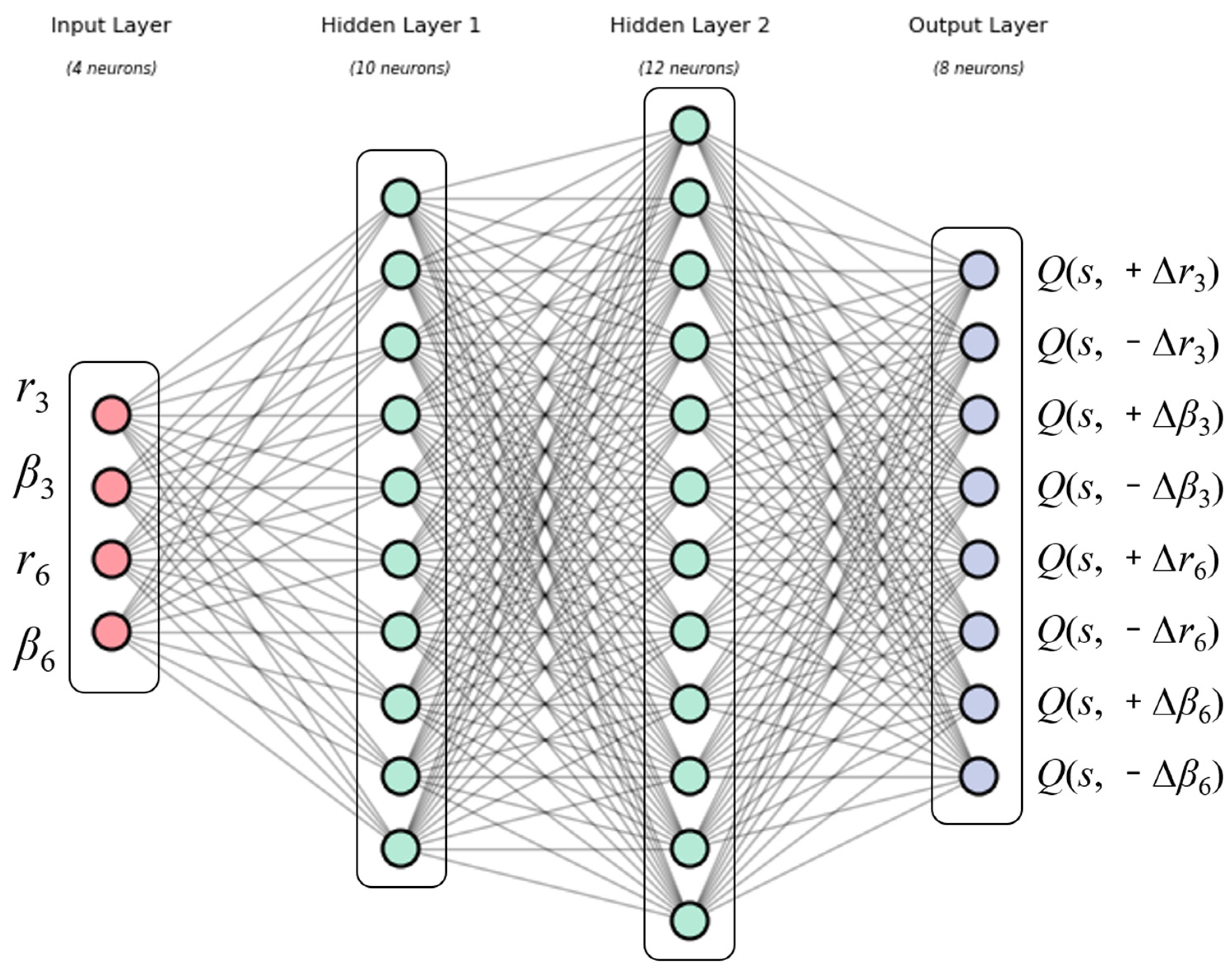
To build a DQN agent for fine-tuning layout optimization, training data preparation and the neural network construction are necessary. To generate sufficient valid datasets as initial input, fine-tuning variables are set in advance. After each fine-tuning action, the entire wind farm layout changes, and power yield and noise radiation have to be re-estimated, the Q-value of the state-action pair is updated. In DQN, the neural network architecture determines the operation of constructing the Q-table. The Q-table is approximated using a DNN with two fully connected hidden layers (10 and 12 neurons per layer, respectively), each using ReLU activation functions, as depicted in Figure 10. The input layer and the output layer have dimensions of 4 and 8, respectively. The four fine-tuning variables and the eight fine-tuning actions for the two turbines are connected to the input and output layers, respectively. Inputs are fed directly into the ANN, and each output variable is normalized to [0, 1]. A limitation of this approach is the absence of dropout or other regularization techniques, as DQN training is notoriously unstable, and introducing dropout would add complexity and potentially compromise stability.

Besides DNN configuration parameters, several hypermeters require tuning during training. These include replay buffer capacity N, reward discount factor γ, delayed steps C for target action-value function update, and ε-greedy factor ε. It is worth noting that the algorithm is highly sensitive to the hyperparameters such as learning rate and discount factor. To obtain a desired hyperparameter setup, tuning these parameters is a tedious and time-consuming task. In this study, given the large hyperparameters space, a grid validation method was used for exploration (γ from 0.05 to 0.3 in steps of 0.05, N from 50 to 400 in steps of 50). The hyperparameter configuration remained fixed across multiple layouts and various wind scenarios. The step-size C for semi-gradient descent used to update the network parameters was set to 0.1. Other training parameters are listed in

Table 1. Training parameters used for the DQN agent.

Parameter	Value
Replay buffer capacity N	200
Reward discount factor γ	0.1
The ε-greedy policy ε	0.8
Learning rate	0.002
Batch size	64
Number of training episodes	500

, the values of γ, ε and learning rate are 0.1, 0.8 and 0.002, respectively and the number of N and batch size is 200 and 64, respectively.

The online DQN neural network was trained using the Adam optimizer, which backpropagates the gradient of the loss value for every component in the neural network’s weights vector. MSE loss was employed. The backpropagation algorithm minimized the loss function starting from the output layer and progressing backward. After training, the optimal weight parameters of the DQN were used to acquire optimized actions.

5.4. Optimization Results

Using the AEP and noise influence area of the original layout as reference, rewards were obtained through iteration. Noted that the AEP of each turbine changes even though only the locations of two fine-tuning turbines are modified. Since subsequent layouts are generated from previous layouts and movements, each adjustment has a small variation. To quickly reach an optimal layout and enhance optimization efficiency, four candidate layouts (Starter 1 to 4) based on the original layout were created as initial schemes. Learning stability was not affected, and more configurations (2, 6 and 8 layouts) were tested.

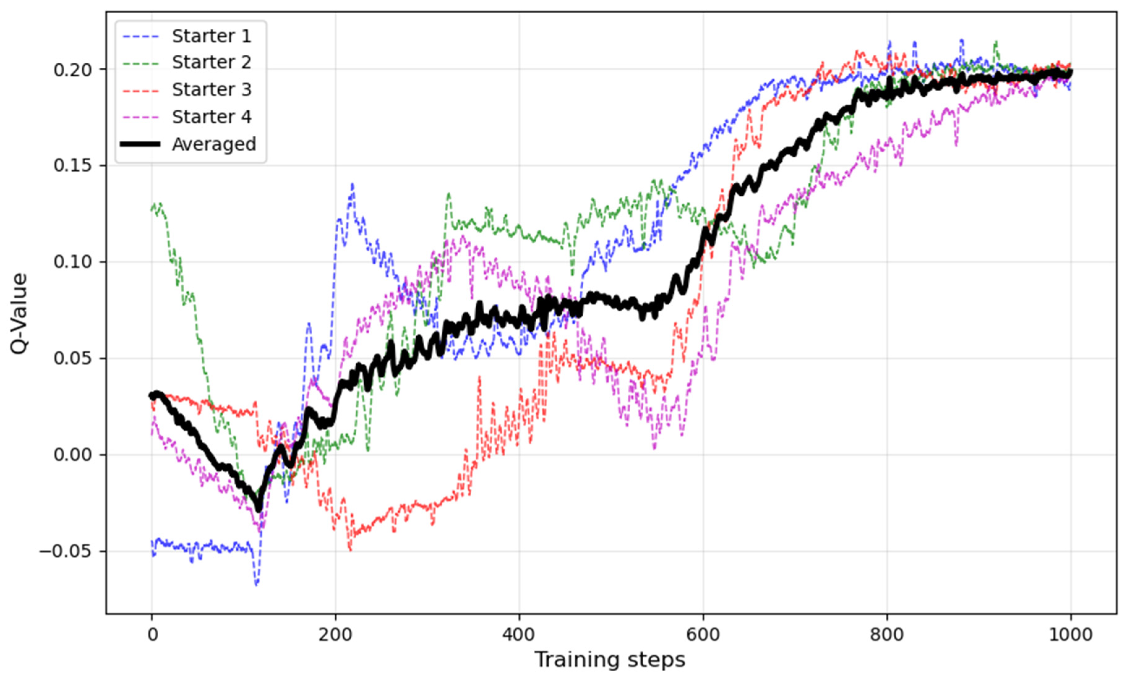
Figure 11 shows their Q-value variation and averaged value during 1000 iterative training steps. Although each starter exhibits different fluctuation patterns, the average reward shows a gradually increasing trend and converges to 0.19 after about step 800. Finally, the agent produces optimized policies, and rewards fluctuate slightly as the DQN continues to choose random actions. The ε-greedy mechanism incorporates exploration during learning. The initial reward is relatively low when ε = 0.8 and it decays linearly over time as the agent explores aggressively. In brief, the results indicate that the proposed approach successfully learned to increase rewards.

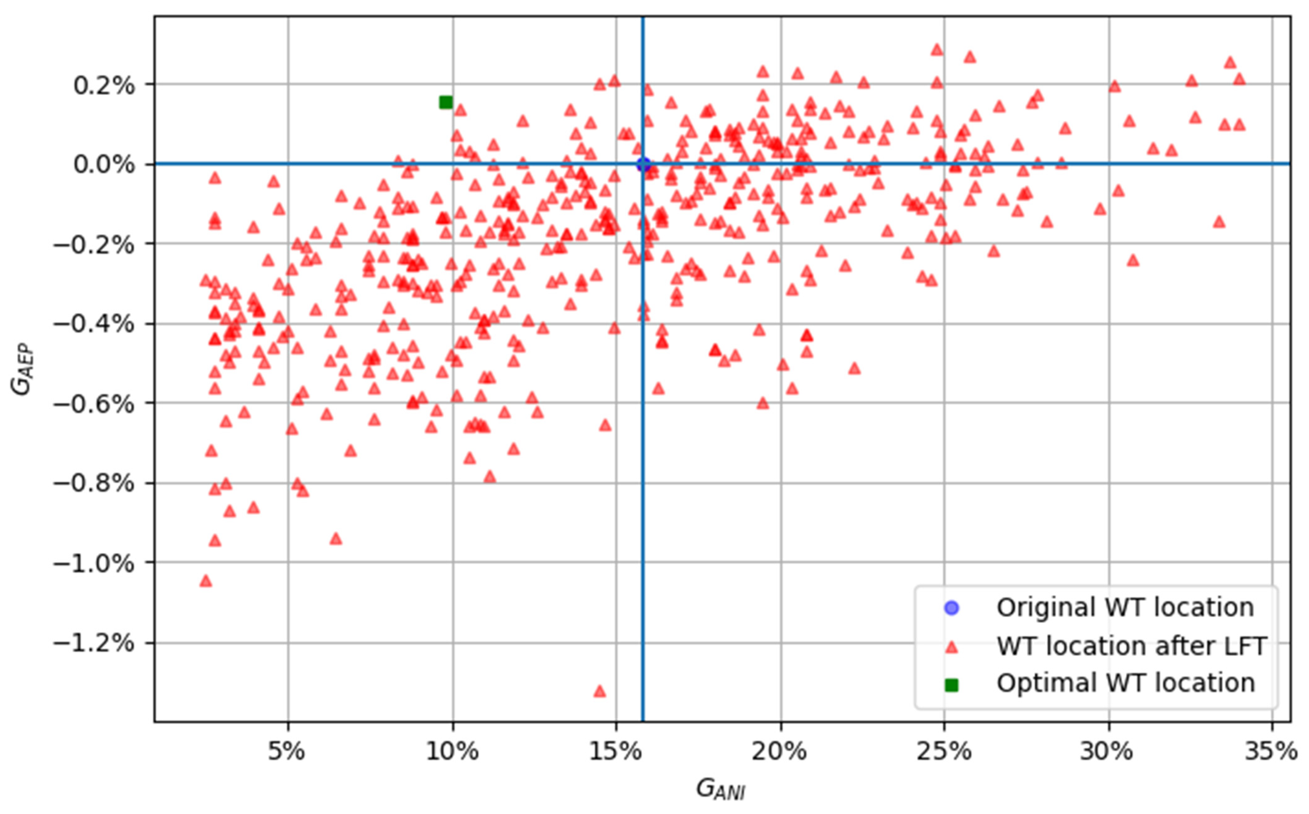
To address the wind farm layout fine-tuning optimization problem, a practical optimization technique is essential. The original layout yielded an AEP of 229.481 GWh, and a G_ANI value of 15.81%. Using this AEP as a baseline, the AEP improvement gain G_AEP of subsequent layouts was calculated. After evaluating 800 different configurations, an optimal WT layout (indicated by a green square in Figure 12) was identified. Compared to the original layout, the optimized scheme achieves a moderately higher AEP (with a G_AEP of 1.6%) and a reduced G_ANI of 9.81%, achieving a subtle balance between energy production and noise contamination. Despite yielding only marginal improvements compared to the original layout, the method ensures high reproducibility, with values showing consistent stability across averaged simulation runs.

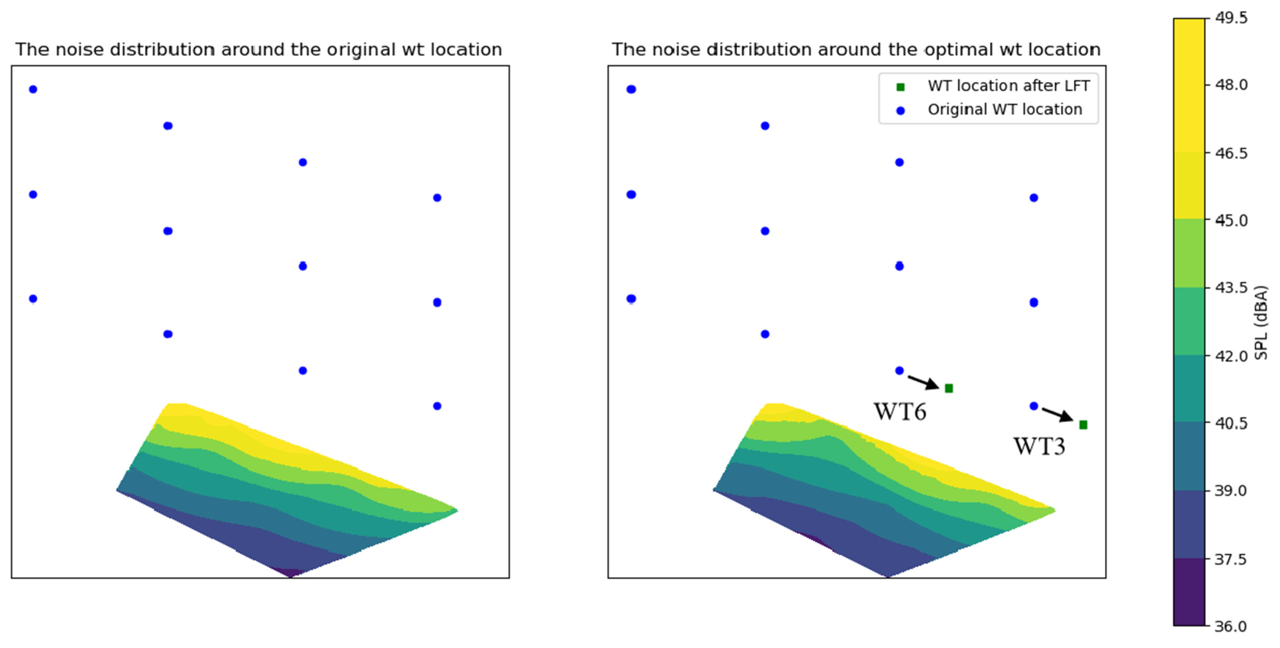
Figure 13 presents the noise distribution in the residential area for both the original and optimized wind farm layouts, respectively. Under the LFT strategy, turbines WT3 and WT6 are relocated toward the bottom-right direction. As a result, the noise-affected area is reduced by 37.95%. The optimal wind farm layout is predominantly influenced by noise considerations.

6. Conclusions

In this study, a data-driven model was developed to facilitate efficient fine-tuning of wind farm layouts. Based on the initial positions of two turbines in an onshore wind farm, complex relationships between turbine arrangement, annual energy production (AEP), and noise-affected area were modeled. By adjusting the locations of these two edge turbines, a balance between power generation and noise control was achieved. Optimization results demonstrate that the proposed method improves the power-noise trade-off compared to the original regular layout, yielding a marginal increase in AEP of 0.16% while reducing the noise-affected area by 6.0%. Although these improvements are modest, they indicate promising potential for larger-scale applications involving more turbines.

The proposed layout adjustment methodology builds on a location fine-tuning strategy supported by a reinforcement learning (RL) model. While initial findings confirm its rationality and effectiveness, several limitations remain. First, the performance of the Deep Q-Network (DQN) is highly sensitive to hyperparameter selection, which involves a tedious and challenging task. Second, to improve practical applicability, real-world constraints such as farm boundaries should be incorporated, and validation with actual wind farm data is necessary. Third, the method should be tested on larger wind farms with more turbines to assess its scalability. Future work will focus on enhancing the robustness of the model through further technical exploration.

The proposed method has been tested on various regular layout shapes under varying wind conditions, and its robustness has been verified through extensive simulations. In summary, this layout adjustment strategy meets the requirements of practical engineering applications and shows significant potential for broader implementation. Machine learning techniques offer a promising pathway to address micro-siting challenges, particularly in optimizing wind farm layouts near residential areas.

References

1. Wisniewski, R.; Soleimanzadeh, M. An Optimization Framework for Load and Power Distribution in Wind Farms: Low Wind Speed. IFAC Proc. Vol. 2011, 44, 5561–5566. [Google Scholar] [CrossRef]
2. Könecke, S.; Hörmeyer, J.; Bohne, T.; Rolfes, R. A New Base of Wind Turbine Noise Measurement Data and Its Application for a Systematic Validation of Sound Propagation Models. Wind. Energy Sci. Discuss. 2022, 8, 639–659. [Google Scholar] [CrossRef]
3. Nyborg, C.M.; Fischer, A.; Thysell, E.; Feng, J.; Søndergaard, L.S.; Sørensen, T.; Hansen, T.R.; Hansen, K.S.; Bertagnolio, F. Propagation of Wind Turbine Noise: Measurements and Model Evaluation. J. Phys. Conf. Ser. 2022, 2265, 032041. [Google Scholar] [CrossRef]
4. Josimović, B.; Bezbradica, L.; Manić, B.; Srnić, D.; Srebrić, N. Cumulative Impact of Wind Farm Noise. Appl. Sci. 2023, 13, 8792. [Google Scholar] [CrossRef]
5. van Kuik, G.A.M.; Peinke, J.; Nijssen, R.; Lekou, D.; Mann, J.; Sørensen, J.N.; Ferreira, C.; van Wingerden, J.W.; Schlipf, D.; Gebraad, P.; et al. Long-Term Research Challenges in Wind Energy—A Research Agenda by the European Academy of Wind Energy. Wind Energy Sci. 2016, 1, 1–39. [Google Scholar] [CrossRef]
6. Veers, P.; Bottasso, C.; Manuel, L.; Naughton, J.; Pao, L.; Paquette, J.; Robertson, A.; Robinson, M.; Ananthan, S.; Barlas, A.; et al. Grand Challenges in the Design, Manufacture, and Operation of Future Wind Turbine Systems; Aerodynamics and hydrodynamics. Wind. Energy Sci. 2022, 8, 1071–1131. [Google Scholar] [CrossRef]
7. Willis, D.J.; Niezrecki, C.; Kuchma, D.; Hines, E.; Arwade, S.R.; Barthelmie, R.J.; DiPaola, M.; Drane, P.J.; Hansen, C.J.; Inalpolat, M.; et al. Wind Energy Research: State-of-the-Art and Future Research Directions. Renew. Energy 2018, 125, 133–154. [Google Scholar] [CrossRef]
8. Zagubień, A.; Wolniewicz, K.; Szwochertowski, J. Analysis of Wind Farm Productivity Taking Wake Loss into Account: Case Study. Energies 2024, 17, 5816. [Google Scholar] [CrossRef]
9. Howland, M.F.; Quesada, J.B.; Martínez, J.J.P.; Larrañaga, F.P.; Yadav, N.; Chawla, J.S.; Sivaram, V.; Dabiri, J.O. Collective wind farm operation based on a. predictive model increases utility-scale energy production. Nat. Energy 2022, 7, 818–827. [Google Scholar] [CrossRef]
10. Silva, J.G.; Ferrari, R.; Wingerden, J.W.V. Wind farm control for wake-loss compensation, thrust balancing and load-limiting of turbines. Renew. Energy 2023, 203, 421–433. [Google Scholar] [CrossRef]
11. Feng, J.; Shen, W.Z. Co-Optimization of the Shape, Orientation and Layout of Offshore Wind Farms. J. Phys. Conf. Ser. 2020, 1618, 042023. [Google Scholar] [CrossRef]
12. Hasager, C.B.; Vincent, P.; Badger, J.; Badger, M.; Di Bella, A.; Peña, A.; Husson, R.; Volker, P.J.H. Using Satellite SAR to Characterize the Wind Flow around Offshore Wind Farms. Energies 2015, 8, 5413–5439. [Google Scholar] [CrossRef]
13. Sickler, M.; Ummels, B.; Zaaijer, M.; Schmehl, R.; Dykes, K. Offshore Wind Farm Optimisation: A Comparison of Performance between Regular and Irregular Wind Turbine Layouts. Wind Energy Sci. 2023, 8, 1225–1233. [Google Scholar] [CrossRef]
14. Tao, S.; Xu, Q.; Andrés Feijóo Zheng, G.; Zhou, J. Nonuniform wind farm layout optimization: A state-of-the-art review. Energy 2020, 209, 118339. [Google Scholar] [CrossRef]
15. Hou, P.; Zhu, J.; Ma, K.; Yang, G.; Hu, W.; Chen, Z. A review of offshore wind farm layout optimization and electrical system design methods. J. Mod. Power Syst. Clean. Energy 2019, 7, 975–986. [Google Scholar] [CrossRef]
16. Nyborg, C.M.; Fischer, A.; Réthoré, P.-E.; Feng, J. Optimization of Wind Farm Operation with a Noise Constraint. Wind Energy Sci. Discuss. 2022, 8, 255–276. [Google Scholar] [CrossRef]
17. Réthoré, P.-E.; Fuglsang, P.; Larsen, G.C.; Buhl, T.; Larsen, T.J.; Madsen, H.A. TOPFARM: Multi-fidelity Optimization of Wind Farms. Wind. Energy 2014, 17, 1797–1816. [Google Scholar] [CrossRef]
18. Pedersen, M.M.; Forsting, A.M.; van der Laan, P.; Riva, R.; Roman, L.A.; Risco, J.C.; Friis-Møller, M.; Quick, J.; Schøler Christiansen, J.P.; Réthoré, P.E.; et al. PyWake 2.5.0: An Open-Source Wind Farm Simulation Tool. DTU Wind, Technical University of Denmark. 2023. Available online: https://gitlab.windenergy.dtu.dk/TOPFARM/PyWake (accessed on 11 January 2025).
19. Wu, X.; Hu, W.; Huang, Q.; Chen, C.; Jacobson, M.Z.; Chen, Z. Optimizing the Layout of Onshore Wind Farms to Minimize Noise. Appl. Energy 2020, 267, 114896. [Google Scholar] [CrossRef]
20. Wolniewicz, K.; Zagubień, A.; Wesołowski, M. Energy and Acoustic Environmental Effective Approach for a Wind Farm Location. Energies 2021, 14, 7290. [Google Scholar] [CrossRef]
21. Mittal, P.; Mitra, K. Micrositing under practical constraints addressing the energy-noise-cost trade-off. Wind Energy 2020, 23, 1905–1918. [Google Scholar] [CrossRef]
22. Thomas, J.J.; Baker, N.F.; Malisani, P.; Quaeghebeur, E.; Sanchez Perez-Moreno, S.; Jasa, J.; Bay, C.; Tilli, F.; Bieniek, D.; Robinson, N.; et al. A comparison of eight optimization methods applied to a wind farm layout optimization problem. Wind Energy Sci. 2023, 8, 865–891. [Google Scholar] [CrossRef]
23. Risco, J.C.; Rodrigues, R.V.; Friis-Møller, M.; Quick, J.; Pedersen, M.M.; Réthoré, P.-E. Gradient-Based Wind Farm Layout Optimization with Inclusion and Exclusion Zones. Wind. Energy Sci. 2024, 9, 585–600. [Google Scholar] [CrossRef]
24. Stanley, A.P.J.; Ning, A. Massive Simplification of the Wind Farm Layout Optimization Problem. Wind. Energy Sci. 2019, 4, 663–676. [Google Scholar] [CrossRef]
25. Kumar, M.; Sharma, A.; Sharma, N.; Sharma, F.B.; Bhadu, M.; Al-Quraan, A. Wind farm layout optimization problem using nature-inspired algorithms. J. Electr. Comput. Eng. 2024, 2024, 9406519. [Google Scholar] [CrossRef]
26. Yang, K.; Deng, X.; Ti, Z.; Yang, S.; Huang, S.; Wang, Y. A Data-Driven Layout Optimization Framework of Large-Scale Wind Farms Based on Machine Learning. Renew. Energy 2023, 218, 119240. [Google Scholar] [CrossRef]
27. Luo, Z.; Luo, W.; Xie, J.; Xu, J.; Wang, L. A New Three-Dimensional Wake Model for the Real Wind Farm Layout Optimization. Energy Explor. Exploit. 2022, 40, 701–723. [Google Scholar] [CrossRef]
28. Li, Y.A. Deep Reinforcement Learning on Wind Power Optimization. In Proceedings of the 2022 International Conference on Networks, Communications and Information Technology (CNCIT), Beijing, China, 17–19 June 2022; IEEE: Piscataway, NJ, USA, 2022; pp. 45–51. [Google Scholar]
29. Yu, X.; Lu, Y. Reinforcement Learning-Based Multi-Objective Differential Evolution for Wind Farm Layout Optimization. Energy 2023, 284, 129300. [Google Scholar] [CrossRef]
30. Bai, F.; Ju, X.; Wang, S.; Zhou, W.; Liu, F. Wind Farm Layout Optimization Using Adaptive Evolutionary Algorithm with Monte Carlo Tree Search Reinforcement Learning. Energy Convers. Manag. 2022, 252, 115047. [Google Scholar] [CrossRef]
31. Yu, X.; Zhang, W. A Teaching-Learning-Based Optimization Algorithm with Reinforcement Learning to Address Wind Farm Layout Optimization Problem. Appl. Soft Comput. 2024, 151, 111135. [Google Scholar] [CrossRef]
32. Feng, J.; Shen, W.Z. Modelling Wind for Wind Farm Layout Optimization Using Joint Distribution of Wind Speed and Wind Direction. Energies 2015, 8, 3075–3092. [Google Scholar] [CrossRef]
33. Salomons, E.M. Computational Atmospheric Acoustics; Springer Science Business Media, B.V.: Dordrecht, The Netherlands, 2001. [Google Scholar]
34. Gilbert, K.E. A numerically stable formulation of the Green’s function parabolic equation: Subtracting the surface-wave pole. JASA Express Lett. 2014, 137, EL8–EL14. [Google Scholar] [CrossRef]
35. Barlas, E.; Zhu, W.J.; Shen, W.Z.; Andersen, S.J. Wind turbine noise propagation modelling: An unsteady approach. The science of making torque from wind. J. Phys. Conf. Ser. 2016, 753, 022003. [Google Scholar] [CrossRef]
36. Barlas, E.; Zhu, W.J.; Shen, W.Z.; Dag, K.; Moriarty, P. Investigation of amplitude modulation noise with a fully coupled wind turbine noise source and advanced propagation model. In Proceedings of the International Conferences of Wind Turbine Noise, Rotterdam, The Netherlands, 2–5 May 2017. [Google Scholar]
37. Barlas, E.; Zhu, W.J.; Shen, W.Z.; Sørensen, J.N.; Kelly, M.; Andersen, S.J. Effect of wind turbine wake on atmospheric sound propagation. Appl. Acoust. 2017, 122, 51–61. [Google Scholar] [CrossRef]
38. ISO 9613-2:1996; Acoustics—Attenuation of Sound during Propagation Outdoors Part 2: General Method of Calculation. International Organization for Standardization: Geneva, Switzerland, 1996.
39. Yang, Y.; Gao, Y.; Ding, Z.; Wu, J.; Zhang, S.; Han, F.; Qiu, X.; Gao, S.; Wang, Y.-G. Advancements in Q-learning Meta-heuristic Optimization Algorithms: A Survey. Wiley Interdiscip. Rev. Data Min. Knowl. Discov. 2024, 14, e1548. [Google Scholar] [CrossRef]
40. Mnih, V.; Kavukcuoglu, K.; Silver, D.; Rusu, A.A.; Veness, J.; Bellemare, M.G.; Graves, A.; Riedmiller, M.; Fidjeland, A.K.; Ostrovski, G.; et al. Human-level control through deep reinforcement learning. Nature 2015, 518, 529–533. [Google Scholar] [CrossRef] [PubMed]
41. King, J.; Fleming, P.; King, R.; Martínez-Tossas, L.A.; Bay, C.J.; Mudafort, R.; Simley, E. Control-Oriented Model for Secondary Effects of Wake Steering. Wind Energy Sci. 2021, 6, 701–714. [Google Scholar] [CrossRef]
42. Sun, Z.; Zhu, W.J.; Shen, W.Z.; Barlas, E.; Sørensen, J.N.; Cao, J.; Yang, H. Development of an Efficient Numerical Method for Wind Turbine Flow, Sound Generation, and Propagation under Multi-Wake Conditions. Appl. Sci. 2019, 9, 100. [Google Scholar] [CrossRef]
43. Leloudas, G.; Zhu, W.J.; Sørensen, J.N.; Shen, W.Z.; Hjort, S. Prediction and Reduction of Noise from a 2.3 MW Wind Turbine. J. Phys. Conf. Ser. 2007, 75, 012083. [Google Scholar] [CrossRef]
Figure 1. Schematic of the sound propagation method.
Energies 18 05019 g001
Figure 2. Schematic diagram of the fine-tuning layout strategy.
Energies 18 05019 g002
Figure 3. Power production of the wind farm before and after LFT under various wind directions.
Energies 18 05019 g003
Figure 4. Wake wind speed contour of the wind farm (a) before and (b) after LFT under wind direction 180°.
Energies 18 05019 g004
Figure 5. Schematic diagram of the fine-tuning DQN framework.
Energies 18 05019 g005
Figure 6. Basic information about the wind farm (a) turbine locations and the resident zone (b) wind resource rose.
Energies 18 05019 g006
Figure 7. General characteristics of the 6.45 MW wind turbine (a) Cp and Ct curves (b) SPL distribution at rated wind speed.
Energies 18 05019 g007
Figure 8. Noise contour of the resident region at 1.5 m height above ground.
Energies 18 05019 g008
Figure 9. Variation of noise with distance at several frequencies.
Energies 18 05019 g009
Figure 10. The DNN-based Q-network architecture.
Energies 18 05019 g010
Figure 11. Average Q-values variation during training history.
Energies 18 05019 g011
Figure 12. Values of GAEP and GANI over 800 different wind farm layouts.
Energies 18 05019 g012
Figure 13. Noise distribution in the resident area for the original wind farm and the final optimal layout.
Energies 18 05019 g013