A Data Protection Method for the Electricity Business Environment Based on Differential Privacy and Federal Incentive Mechanisms

Abstract

In the development process of the power industry, accurately assessing the level of development of the electricity business environment is of great significance. However, traditional evaluation systems have limitations, with the issue of “data silos” being prominent, and user privacy under federated learning is also at risk. This paper proposes a federated learning-based data protection method for the electricity business environment to address these challenges. Based on the World Bank’s B-READY framework, this paper constructs an electricity business environment evaluation system containing nine indicators, focusing on three aspects: electricity regulations, public services, and operational efficiency. The indicators are weighted using the Sequence Relation and Entropy Weight Method. To address the issue of sensitive data protection, we first use federated learning technology to build a distributed modeling framework, ensuring that raw data never leaves the local environment during the collaborative modeling process. Next, we embed a differential privacy mechanism in the model parameter transmission stage, encrypting the model parameters by adding controlled noise. Finally, an incentive mechanism based on contribution quantification is implemented to encourage participation from all parties. This paper conducts experiments using the data of Shenzhen City, Guangdong Province. Compared with the FNN model and the SVR model, the MLP model reduces MAE by 78.9% and 94.12%, respectively, and increases R² by 37.95% and 55.62%, respectively. The superiority of the method proposed in this paper has been proved.

1. Introduction

With the continuous promotion of new power system construction and the application of a large number of distributed energy sources [1,2], the optimization of the power business environment, as a key step in the reform of “decentralization and management service” in the energy field, has become an important entry point to improve the power supply system and improve the quality of public services. The World Bank’s B-READY evaluation framework proposes a three-dimensional evaluation paradigm of “regulatory framework-public services-efficiency” [3], optimizing the electricity business environment by improving municipal utility coordination, the convenience of electricity access, the reliability of power supply, and electricity access satisfaction. In combination with policy research, it enhances its influence and competitiveness [4,5,6], posing a fundamental challenge to the existing electricity business environment system. Traditional methodologies demonstrate substantial limitations, particularly in domains involving multi-party collaborative service frameworks and the integration of heterogeneous data elements.

The traditional electricity business environment evaluation system has significant shortcomings. The factors it considers are relatively simplistic, often limited to basic aspects such as the electricity connection process, time, cost, supply reliability, and transparency of electricity tariffs. It fails to adequately incorporate important factors like environmental and social impacts, making it difficult to comprehensively and accurately describe the development level of the electricity business environment. As a result, the evaluation outcomes cannot provide precise and effective support for policy formulation and industry development, hindering the optimization process of the electricity business environment. The weights of the indicators in the electricity business environment evaluation system are not equal, and determining the appropriate weights is a key issue. Conventional weighting methodologies are systematically classified into two distinct paradigms: subjective and objective approaches. Subjective weighting techniques exhibit an inherent dependence on domain-specific expertise, thereby introducing substantial variability in the resultant weights due to evaluator subjectivity and cognitive biases. In contrast, objective weighting algorithms frequently fail to adequately account for inter-indicator heterogeneity while demonstrating pronounced sensitivity to input data perturbations, consequently yielding non-robust evaluation outcomes. Xiao Yong et al. [7] developed a risk evaluation system to address safety issues in energy storage station batteries, using the AHP (Analytic Hierarchy Process) and entropy weight methods to calculate combined weights. Using the Sequence Relationship Method and CRITIC method, Wang Mengfan et al. [8] determined combined weights for comprehensive distribution network reliability indicators.

Additionally, data privacy issues have become a key factor hindering the development of the electricity business environment. As electricity data continues its explosive surge, the issue of “data silos” is becoming increasingly grave. Federated learning technology effectively solves the “data silo” problem [9,10]. It empowers participants to co-develop models while preserving data residency within their native domains. Although federated learning protects privacy by sharing model parameters rather than the original data, it is still possible to infer sensitive information through model parameters [11,12]. Consequently, implementing privacy-preserving mechanisms becomes imperative to rigorously safeguard client data confidentiality throughout the data processing pipeline.

Although both homomorphic encryption and differential encryption can achieve privacy protection, homomorphic encryption increases computational complexity. Although there are some algorithms that can effectively perform this kind of calculation (such as the Paillier algorithm), differential privacy has more advantages in computational efficiency compared with homomorphic encryption. Therefore, in scenarios with high real-time requirements such as power operation environment assessment, we have adopted the privacy protection technology of differential privacy. Differential privacy, as a technology with strong privacy protection capabilities [13,14], has been extensively utilized across the domain of data privacy protection in recent years. It primarily works by adding random noise (such as Laplace noise [15] or Gaussian noise [16,17]) to hide the actual results of data query operations, effectively reducing data leakage risk. Given its strong data protection capabilities [18], an increasing number of studies have incorporated it into federated learning, achieving significant results in areas such as smart grids and healthcare. Within the smart grid domain, research [19] has developed a novel photovoltaic grid-connected power forecasting framework that unifies federated learning and differential privacy in a privacy-utility co-optimization framework. This method effectively addresses two critical challenges: (1) preserving data privacy while maintaining model utility and (2) handling non-independent and identically distributed data characteristics inherent in distributed energy systems. In the healthcare field, Choudhury et al. [20] combined federated learning and differential privacy to process health data, effectively safeguarding medical data privacy through a two-layer protection mechanism. Ref. [21] devised a confidentiality-preserving architecture fusing federated and transfer learning, assessing HVAC control efficacy across heterogeneous buildings while resolving data scarcity and privacy risks.

Studies [19,20] lacked a consideration of disparities in data volume and integrity, as well as the contribution among the participants in federated learning. In operational federated learning systems, client contributions demonstrate inherent heterogeneity. Without proper incentive mechanisms, this diversity often leads to suboptimal participation rates. Such participant disengagement ultimately impairs both the convergence efficiency and model performance of the federated framework. Currently, in research on measuring participant contributions, Wang Guan et al. [22] used deletion diagnostics and influence functions to assess the data quality and contribution of different participants. Kang et al. [23] quantitatively assessed participant device resource consumption in federated learning systems by evaluating key parameters including CPU frequency and local model iteration count. These specific metrics provide an objective basis for measuring individual contributions to the federated learning process.

In summary, in the development of the power industry, the data protection of the power consumption business environment faces multiple challenges: (1) The traditional centralized processing mode leads to the risk of privacy leakage when data is shared, and parameter transmission under the federated learning framework may still be subject to inference attacks. (2) The current system takes into account only a single factor and fails to fully incorporate important factors such as environmental and social impacts, making it difficult to comprehensively and accurately describe the development level of the electricity business environment. (3) There are differences in the contribution levels of the participants in federated learning, and there is a lack of effective incentive mechanisms.

To address the above issues, based on the World Bank’s B-READY framework, this paper considers from three perspectives, electricity regulations, public services, and operational efficiency, and it obtains a comprehensive evaluation system for the electricity business environment that takes into account multiple factors and adapts to modern international development standards. The evaluation system consists of a total of nine indicators. The Sequence Relation Method and Entropy Weight Method are used to assign combined weights to the various indicators in the electricity business environment evaluation system. A federated learning-based data protection method for the electricity business environment is proposed. This method collaboratively constructs a high-performance model among all participants, calculates the scores of each indicator in the electricity business environment evaluation system, and assesses the development level of the electricity business environment in a certain region. The main contributions of this paper are as follows:

(1)

A comprehensive electricity business environment evaluation system has been developed, which considers multiple dimensions, including electricity regulations, public services, and operational efficiency. This system can comprehensively and accurately describe the development level of the electricity business environment to adapt to international trends.

(2)

A data protection method for the electricity consumption business environment based on federated learning is proposed. This method, on the basis of traditional federated learning, introduces differential privacy and federated learning incentive mechanisms to solve the data leakage risk of centralized training.

(3)

Experimental verification shows that due to the introduction of the incentive mechanism, MAE, MSE, and RMSE have decreased by 10.36%, 19.31%, and 10.84%, respectively, and R² has increased by 14.05%. Compared with the FNN model and the SVR model, the MLP model reduced MAE by 78.9% and 94.12%, respectively, MSE by 96.86% and 99.27%, respectively, RMSE by 82.15% and 94.31%, respectively, and R² by 37.95% and 55.62%, respectively.

This paper’s organizational framework is structured as follows: Section 2 establishes a novel electricity business environment evaluation system and determines the weights of the indicators within the system. Section 3 primarily presents the theoretical frameworks of federated learning and its main process for application in electricity business environment evaluation. Section 4 verifies the efficacy of the proposed approach and conducts a sensitivity analysis of electricity business environment metrics. Finally, Section 5 concludes by synthesizing the core research outcomes.

2. Electricity Business Environment

2.1. Construction of the Electricity Business Environment Evaluation System

Traditional electricity business environment evaluation methods only consider factors such as the electricity connection process, time, cost, supply reliability, and tariff transparency. These factors are limited and fail to adequately account for environmental and social impacts, rendering it problematic to accurately specify the development level of the electricity business environment. To achieve a timely and precise evaluation of regional electricity business environments, this study adopts the World Bank’s B-READY framework. The assessment system incorporates three critical dimensions: electricity regulations, public services, and operational efficiency. This leads to an electricity business environment indicator evaluation system that considers multiple factors and is adaptable to modern international development. The evaluation system includes three first-level indicators and 9 second-level indicators, as shown in

Table 1. The 9 indicators in the electricity business environment evaluation system.

Primary Indicator	Secondary Indicator
Electricity regulation quality indicator	Collaborative planning and infrastructure development $X_1$
	Regulatory inspection framework for electrical setups $X_2$
	Ecological sustainability in power supply operations $X_3$
Public service quality indicator	KPI for monitoring service reliability and sustainability $X_4$
	Transparency in electricity rate determination and tariff structure $X_5$
	Online power connection request systems $X_6$
Electricity service operational efficiency indicator	Average customer outage time $X_7$
	Average frequency of customer outages $X_8$
	Electricity connection service $X_9$

.

2.1.1. Electricity Regulation Quality Indicator

The regulatory quality index for electricity is principally utilized to gauge the integrity of regulatory systems within power supply entities and their governing authorities. It comprises three sub-indicators as follows.

The electricity regulation quality indicator is primarily used to assess the completeness of the regulatory system of power supply companies and their regulatory authorities. It consists of the following three secondary indicators.

• Collaborative planning and infrastructure development $X_1$

Indicator $X_1$ is rated according to the satisfaction of the following evaluation criteria:

The indicator $X_1$ is scored based on the fulfillment of the following criteria:

• Statutory provisions require collaborative planning and infrastructure development with shared excavation permits and one-time digging policies.
• The regulations set time limits for approval/consent by the electricity connection authority.

The calculation formula for the score of this indicator is shown in Formula (1):

$$X_1=50({\lambda }_{1\mathrm{a}}+{\lambda }_{1\mathrm{b}})$$

(1)

where $X_1$ indicates the score of the indicator collaborative planning and infrastructure development; ${\lambda }_{1\mathrm{a}}, {\lambda }_{1\mathrm{b}}$ denote compliance statuses of standards a/b within the assessed region, and ${\lambda }_{1\mathrm{a}}, {\lambda }_{1\mathrm{b}}\in \left\{0,1\right\}$. A value of 1 is assigned when requirements are met, and 0 otherwise. Subsequent parameters structured as ${\lambda }_{ij}$ adhere to this binary protocol, representing the j-th criterion under the i-th indicator.

2.

Regulatory inspection framework for electrical setups $X_2$

The indicator $X_2$ encompasses two elements: internal and external installation works. The internal component’s evaluation is determined by adherence to specific criteria:

The indicator $X_2$ consists of two parts, the internal installation works and the external installation works. The internal installation work component is scored based on the fulfillment of the following criteria:

• The law mandates licensed professionals/companies to install and certify internal electrical systems.
• Legal requirements enforce external, independent auditing of on-premise electrical setup work.

The calculation formula for the score of internal installation projects is shown in Formula (2):

$$X_{21}=\left\{\begin{array}{c}50,\left({\lambda }_{2\mathrm{a}}+{\lambda }_{2\mathrm{b}}\right)\ge 1\\ 0,\left({\lambda }_{2\mathrm{a}}+{\lambda }_{2\mathrm{b}}\right)<1\end{array}\right\}$$

(2)

where $X_{21}$ quantifies the internal installation metric within the electrical inspection system indicator; ${\lambda }_{2\mathrm{a}},{\lambda }_{2\mathrm{b}}$ designate compliance statuses for benchmarks a and b in the target assessment zone.

The exterior installation segment gets a score determined by meeting the subsequent criteria:

• The law mandates licensed professionals/companies to install and certify external electrical systems.
• Statutes mandate third-party examination of outdoor electrical fitting setups.

The calculation formula for the score of external installation projects is shown in Formula (3):

$$X_{22}=\left\{\begin{array}{c}50,\left({\lambda }_{2\mathrm{c}}+{\lambda }_{2\mathrm{d}}\right)\ge 1\\ 0,\left({\lambda }_{2\mathrm{c}}+{\lambda }_{2\mathrm{d}}\right)<1\end{array}\right\}$$

(3)

where $X_{22}$ quantifies the external installation element within the electrical inspection system indicator; ${\lambda }_{2\mathrm{c}},{\lambda }_{2\mathrm{d}}$ reflect compliance attainment for criteria c and d in the designated assessment zone.

The scoring formula corresponding to this indicator is presented in Formula (4):

$$X_2=X_{21}+X_{22}$$

(4)

The $X_2$ denotes the score assigned to the regulatory inspection framework for electrical setups indicator.

3.

Ecological sustainability in power supply operations $X_3$

The indicator $X_3$ consists of two components: the electricity production sector and the grid delivery infrastructure. The generation unit is evaluated according to the fulfillment of these benchmarks:

• The regulations set environmental standards for power generation, including energy efficiency and limits on air pollutants.
• The regulatory framework enforces power generation environmental compliance through penalties and mandatory reporting.

The calculation formula for this part of the score is shown in Formula (5):

$$X_{31}=\left\{\begin{array}{c}50,\left({\lambda }_{3\mathrm{a}}+{\lambda }_{3\mathrm{b}}\right)=2\\ 25,\left({\lambda }_{3\mathrm{a}}+{\lambda }_{3\mathrm{b}}\right)=1\\ 0,\left({\lambda }_{3\mathrm{a}}+{\lambda }_{3\mathrm{b}}\right)=0\end{array}\right\}$$

(5)

where $X_{31}$ quantifies the ecological sustainability metric within power generation systems, and ${\lambda }_{3\mathrm{a}}, {\lambda }_{3\mathrm{b}}$ reflect performance attainment levels for benchmarks a and b in the designated assessment zone.

The electricity transmission—distribution section is graded according to the fulfillment of the following standards:

c.

The regulatory framework mandates environmental standards for transmission and distribution, including energy efficiency, smart meters, and smart grid development.

d.

The regulatory framework establishes pertinent environmental criteria for power delivery and allocation.

The calculation formula for this part of the score is shown in Formula (6):

$$X_{32}=\left\{\begin{array}{c}\hfill 50,\left({\lambda }_{3\mathrm{c}}+{\lambda }_{3\mathrm{d}}\right)=2\\ \hfill 25,\left({\lambda }_{3\mathrm{c}}+{\lambda }_{3\mathrm{d}}\right)=1\\ \hfill 0,\left({\lambda }_{3\mathrm{c}}+{\lambda }_{3\mathrm{d}}\right)=0\end{array}\right\}$$

(6)

where $X_{32}$ quantifies ecological impact metrics within transmission and distribution systems, and ${\lambda }_{3\mathrm{c}},{\lambda }_{3\mathrm{d}}$ reflect compliance status for benchmarks c and d in designated assessment sectors.

The scoring formula corresponding to this indicator is presented in Formula (7):

$$X_3=X_{31}+X_{32}$$

(7)

$X_3$ denotes the score assigned to the indicator ecological sustainability in power supply operations.

2.1.2. Public Service Quality Indicator

The public service level indicator serves as a quantitative assessment framework designed to evaluate both the service governance efficacy of power supply institutions and enterprises and the disclosure transparency of public service facilities. It comprises three sub-indicators as follows.

• KPI for monitoring service reliability and sustainability $X_4$

The indicator $X_4$ gets a score determined by meeting the following criteria:

• There are core performance metrics for tracking the dependability of the power supply.
• There are core performance metrics to gauge the environmental viability of power delivery.

The scoring formula corresponding to this indicator is presented in Formula (8):

$$X_4=50\left({\lambda }_{4\mathrm{a}}+{\lambda }_{4\mathrm{b}}\right)$$

(8)

where $X_4$ quantifies the KPI for monitoring service reliability and sustainability; ${\lambda }_{4\mathrm{a}}, {\lambda }_{4\mathrm{b}}$ signify compliance attainment levels for benchmarks a and b within designated evaluation zones.

2.

Transparency in electricity rate determination and tariff structure $X_5$

The indicator $X_5$ can attain a score dependent on the accomplishment of the herein-specified standards:

• The regional electricity tariff is publicly available via the utility or regulator’s official online platform.
• Electricity price changes are announced to the public at least one invoicing period prior.
• The methodology for determining users’ final power utility bill is publicly disclosed.

The scoring formula corresponding to this indicator is presented in Formula (9):

$$X_5=\left\{\begin{array}{c}\hfill 100,\left({\lambda }_{5\mathrm{a}}+{\lambda }_{5\mathrm{b}}+{\lambda }_{5\mathrm{c}}\right)=3\\ \hfill \left(100\ast 2\right)/3,\left({\lambda }_{5\mathrm{a}}+{\lambda }_{5\mathrm{b}}+{\lambda }_{5\mathrm{c}}\right)=2\\ \hfill 100/3,\left({\lambda }_{5\mathrm{a}}+{\lambda }_{5\mathrm{b}}+{\lambda }_{5\mathrm{c}}\right)=1\end{array}\right\}$$

(9)

where $X_5$ indicates the score of the transparency in electricity rate determination and tariff structure; ${\lambda }_{5\mathrm{a}},{\lambda }_{5\mathrm{b}},{\lambda }_{5c}$ indicate the fulfillment of criteria a, b, and c, respectively, in the scoring target area.

3.

Online power connection request systems $X_6$

The indicator $X_6$ gets a score according to the fulfillment of the subsequent standards:

• Businesses can electronically request new commercial power connections.
• Users can track their power connection application progress online.

The scoring formula corresponding to this indicator is presented in Formula (10):

$$X_6=\left\{\begin{array}{c}\hfill 100,\left({\lambda }_{6\mathrm{a}}+{\lambda }_{6\mathrm{b}}\right)=2\\ \hfill 50,\left({\lambda }_{6\mathrm{a}}+{\lambda }_{6\mathrm{b}}\right)=1\\ \hfill 0,\left({\lambda }_{6\mathrm{a}}+{\lambda }_{6\mathrm{b}}\right)=0\end{array}\right\}$$

(10)

where $X_6$ quantifies the online application tracking capability for power connection services; ${\lambda }_{6\mathrm{a}}, {\lambda }_{6\mathrm{b}}$ validate compliance attainment levels for standards a and b within prescribed assessment zones.

2.1.3. Electricity Service Operational Efficiency Indicator

The business electricity acquisition efficiency indicator functions as a holistic metric to gauge power supply procurement reliability and operational costs of sustaining electricity supply in practice. It comprises three sub-indicators as follows.

• Average customer outage time $X_7$

The scoring formula corresponding to this indicator is presented in Formula (11):

$$X_7={\displaystyle \frac{SAIDI\_g-SAIDI}{SAIDI\_g-SAIDI\_b}}\ast 100$$

(11)

where $X_7$ is the score for the average customer outage time; $SAIDI\_\mathrm{g}$ is the optimal value for the average customer outage time in a month, taken as 0; $SAIDI\_\mathrm{b}$ is the worst value for the average customer outage time in a month, taken as 0.31; and $SAIDI$ is the average customer outage time for that month. The calculation formula is shown in Formula (12):

$$SAIDI={\displaystyle \frac{{\displaystyle \sum \left(\mathrm{t}\ast \mathrm{n}\right)}}{N}}$$

(12)

t represents the duration of a single power outage within a month, n counts affected customers in the event, and N represents the overall number of electricity customers.

2.

Average frequency of customer outages $X_8$

The scoring formula corresponding to this indicator is presented in Formula (13):

$$X_8={\displaystyle \frac{SAIFI\_g-SAIFI}{SAIFI\_g-SAIFI\_b}}\ast 100$$

(13)

where $X_8$ is the score for the average customer outage frequency; $SAIFI\_\mathrm{g}$ is the optimal value for the average customer outage frequency in a month, taken as 0; $SAIFI\_\mathrm{b}$ is the worst value for the average customer outage frequency in a month, taken as 1.66; and $SAIFI$ is the average customer outage frequency for that month. The calculation formula is shown in Formula (14):

$$SAIFI={\displaystyle \frac{{\displaystyle \sum \mathrm{n}}}{N}}$$

(14)

n denotes monthly outages’ affected customer quantity, and N represents the overall number of electricity customers.

3.

Electricity Connection Service $X_9$

The scoring formula corresponding to this indicator is presented in Formula (15):

$$X_9={\displaystyle \frac{F_b-F}{F_b-F_g}}\ast 100$$

(15)

where $X_9$ is the score for the electricity connection service indicator; $F_{\mathrm{g}}$ is the optimal electricity connection cost coefficient, taken as 10; $F_{\mathrm{b}}$ is the worst electricity connection cost coefficient, taken as 50; and $F$ is the electricity connection service cost coefficient. The calculation formula is presented in (16):

$$F={\displaystyle \frac{E}{R}}$$

(16)

where E signifies the cumulative yearly power expenditure for a user with a voltage of 10 KV and load capacity of 180 KVA. R denotes the aggregate annual net income of residents in the area.

2.2. Determination of Indicator Weights

The Sequence Relationship Method is a subjective weighting method that first ranks the evaluation indicators qualitatively based on expert scores and then assigns quantitative values. The Entropy Method can deeply reflect the utility value of the indicator’s information entropy, overcoming the subjectivity of the Sequence Relationship Method to improve the credibility and accuracy of the indicator weights. Given the characteristics of these two methods, in order to make the determination of weights more reasonable and accurate, this paper combines the Sequence Relationship Method and the Entropy Method to determine the weights of the 9 indicators.

2.2.1. Entropy Weight Method for Calculating Objective Weights

The Entropy Weight Method, as an objective weighting approach, assigns proportionally higher weights to indicators demonstrating lower information entropy values, since these indicators exhibit more significant variability and consequently contain richer informational content. Conversely, indicators with higher information entropy should be assigned lower weights. The steps for calculating the objective weights of the 9 indicators in this article are as follows.

Step 1: Obtain the raw data matrix. Suppose there are n evaluation indicators and m sets of data. Then, the raw data matrix R can be represented as

$$R=\left[\begin{array}{cccc}{r}_{11}& r_{12}& \cdots & r_{1n}\\ & & & \\ r_{21}& r_{22}& \cdots & r_{2n}\\ ⋮& ⋮& \ddots & ⋮\\ & & & \\ r_{m1}& r_{m2}& \cdots & r_{mn}\end{array}\right]$$

(17)

Step 2: Normalize the raw data matrix. Perform dimensional normalization for each indicator to eliminate units, and then apply translation correction to obtain the corresponding matrix $R_0^{\mathrm{norm}}$.

$${\mathrm{r}}_{\mathrm{ij}}^{\mathrm{norm}}={\displaystyle \frac{\mathrm{r}-{\mathrm{r}}_{\min }}{{\mathrm{r}}_{\max }-{\mathrm{r}}_{\min }}}$$

(18)

$$\begin{array}{c}{R}_0^{norm}=\left[\begin{array}{cccc}{r}_{11}^{norm}+\epsilon & r_{12}^{norm}+\epsilon & \cdots & r_{1n}^{norm}+\epsilon \\ r_{21}^{norm}+\epsilon & r_{22}^{norm}+\epsilon & \cdots & r_{2n}^{norm}+\epsilon \\ ⋮& ⋮& \ddots & ⋮\\ r_{m1}^{norm}+\epsilon & r_{m2}^{norm}+\epsilon & \cdots & r_{mn}^{norm}+\epsilon \end{array}\right]=\\ \left[\begin{array}{cccc}{R}_{11}^{norm}& R_{12}^{norm}& \cdots & R_{1n}^{norm}\\ R_{21}^{norm}& R_{22}^{norm}& \cdots & R_{2n}^{norm}\\ ⋮& ⋮& \ddots & ⋮\\ R_{m1}^{norm}& R_{m2}^{norm}& \cdots & R_{mn}^{norm}\end{array}\right]\end{array}$$

(19)

where ${\mathrm{r}}_{\mathrm{ij}}^{\mathrm{norm}}$ is the normalized data; ε is a small value approaching 0; $R_0^{\mathrm{norm}}$ is the corrected data.

Step 3: Solve for the weight $P_{ij}$

$$p_{ij}={\displaystyle \frac{R_{ij}^{norm}}{{\displaystyle \sum _{i=1}^m}{R}_{ij}^{norm}}}$$

(20)

Step 4: Solve for the information entropy $e_j$.

$$e_j=-K\times \sum _{i=1}^m\left(p_{ij}\ln p_{ij}\right)$$

(21)

where $K=1/\left(\ln m\right)$.

Step 5: Calculate the degree of variability $G_j$.

$$G_j=1-e_j$$

(22)

Step 6: Solve for the entropy weight.

$$w_j^{*}={\displaystyle \frac{G_j}{{\displaystyle \sum _{j=1}^n}{G}_j}}$$

(23)

$$W^{\mathrm{a}}=\left(w_1^{*},w_2^{*},\cdots ,w_n^{*}\right)$$

(24)

2.2.2. Sequence Relationship Method for Calculating Subjective Weights

The Sequence Relationship Method is a subjective weighting method. Compared to the Analytical Hierarchy Process (AHP) for determining weights, it is not limited by the number of evaluation elements, does not require consistency checks, and is simple to compute and highly operable. The steps for calculating the subjective weights of the 9 indicators in this paper are as follows.

Step 1: Rank the importance of the indicators. G₁, G₂, …, G_n represent the various indicators.

Step 2: Quantify the importance of the indicators. Subject matter experts are engaged to conduct pairwise comparisons of the pre-ranked indicators, assigning quantified importance scores based on their professional judgment.

$$r_k={\displaystyle \frac{{\omega }_{k-1}}{{\omega }_k}}(k=n,n-1,\cdots 2,1)$$

(25)

where n denotes total evaluation indicators, ${\omega }_k$ represents the k-th indicator’s weight, and $r_k$ signifies the importance ratio of adjacent indicators.

Step 3: Calculate the weights for each indicator.

$$w_k={\left(1+\sum _{n=2i=n}^k\prod _{i=n}^k{r}_i\right)}^{-1}$$

(26)

where $r_i$ is the rational value assigned by the expert to the i-th indicator.

Step 4: Determine the weights of the remaining indicators. The formula is as follows:

$${\omega }_{k-1}=r_k{\omega }_k,(k=n,n-1,\cdots 2,1)$$

(27)

$$W^b=\left(w_1,w_2,\cdots ,w_n\right)$$

(28)

2.2.3. Combined Weight Calculation

After determining the subjective and objective weights of the nine indicators by using the above two methods, the combined weights of the nine indicators were solved by using the coefficient of difference method. The formula is as follows:

$$W_i=\alpha W_i^a+\beta W_i^b$$

(29)

where $W_i$ is the combined weight of a certain indicator; $W_i^a$ is the objective weight; $W_i^b$ is the subjective weight; α and β are the subjective and objective linear coefficients.

The calculation formulas for subjective weight and objective weight coefficients are as follows:

$$\left\{\begin{array}{l}\alpha ={\displaystyle \frac{\mathrm{n}}{n-1}}\left({\displaystyle \frac{2}{n}}{\displaystyle \sum _{i=1}^{n}n{G}_i}-{\displaystyle \frac{n+1}{n}}\right)\\ \alpha =1-\beta \end{array}\right.$$

(30)

where G_i is the subjective weight arranged in ascending order, and n denotes the quantity of indicators.

The calculation of the total score for electricity business environment indicators is shown below:

$$X={\displaystyle \sum _{i=1}^9{W}_i{X}_i}$$

(31)

where X denotes the total score of electricity business environment indicators, and X_i signifies the i-th indicator score.

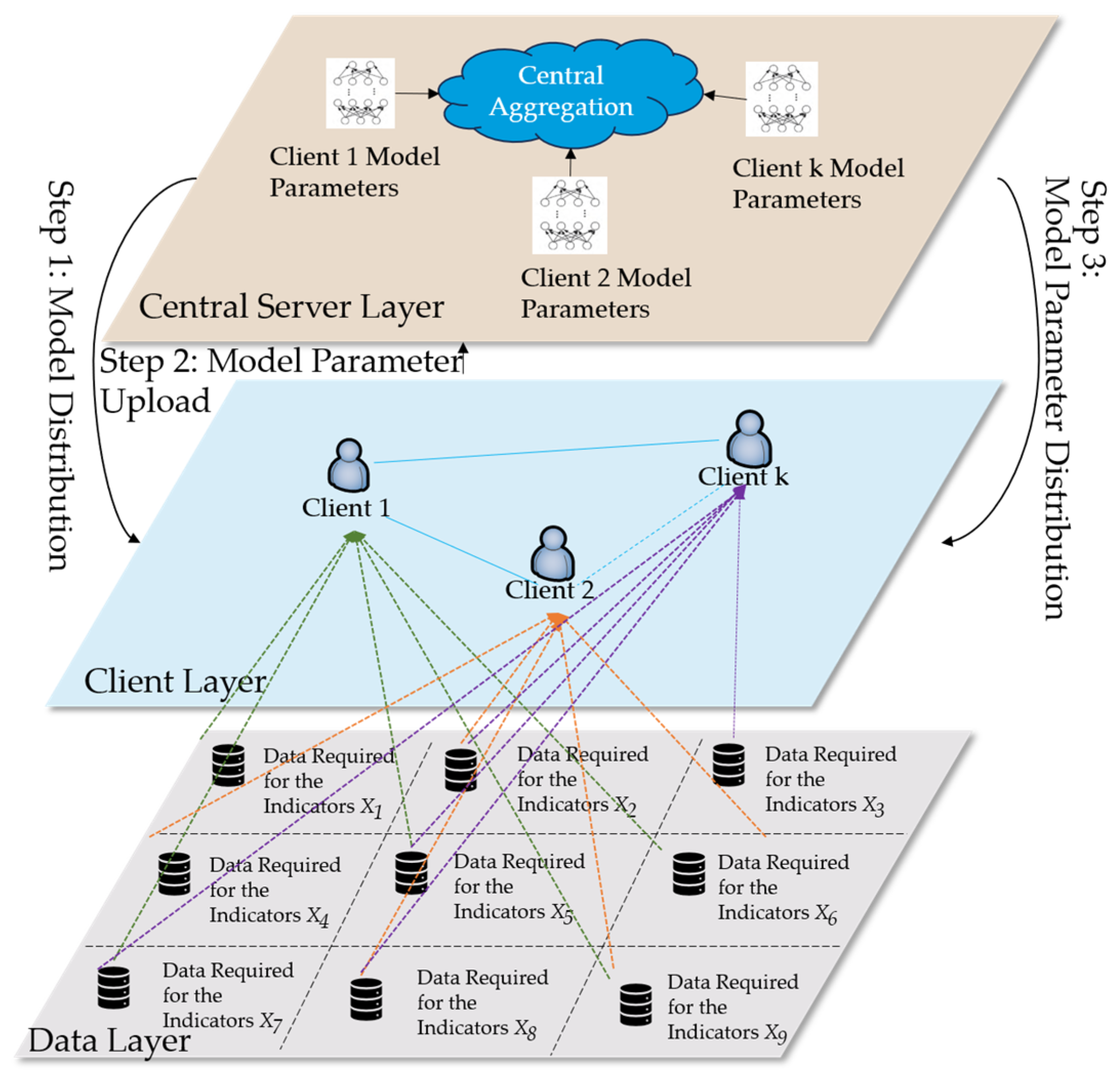
3. Federated Learning

Federated learning is a distributed machine learning paradigm enabling collaborative model training among multiple participants. During training, it keeps all datasets local, removing the need for direct data sharing. Thus, it offers an effective solution to meet strict data privacy protection demands in machine learning applications. Based on data distribution features, federated learning splits into three modes: horizontal, vertical, and transfer learning. This paper adopts horizontal federated learning, which mainly tackles the “data silo” problem. Evaluating electricity business environments involves decentralized datasets from multiple power firms. These distributed data sources often hold commercially sensitive and proprietary info. Traditional centralized processing approaches carry a privacy leakage risk. Horizontal federated learning adopts a federated learning mode of local training and global aggregation. After the model training is computed locally on the client side, only the updated values of the model parameters are uploaded, and the original data does not leave the local device, achieving multi-party collaborative training. It not only protects data privacy but also utilizes data from all parties to optimize the evaluation effectiveness of the electricity consumption business environment, promoting the development of the electricity consumption business environment evaluation system.

3.1. Horizontal Federated Learning Framework

The electricity business environment evaluation indicators cover cross-departmental, multi-dimensional data (such as regulatory compliance, outage frequency, electricity tariff transparency, etc.), which are distributed across different power companies and contain sensitive information (such as user electricity consumption behavior). Different power companies possess varying amounts and dimensions of data. Therefore, this paper uses horizontal federated learning to perform collaborative modeling for indicator calculation and analysis, without sharing raw data among the companies.

The federated learning framework for the electricity business environment evaluation system is shown in Figure 1. The methodology comprises three key steps: (1) The central server initializes global model params and sends the initial model to clients. (2) Each client trains the model using distributed model parameters and proprietary datasets and then transmits the updated parameters to the server for integration. (3) After aggregating local update parameters from clients, the server replaces the global model with the averaged model and sends updated global model parameters back to clients for the next training round—enabling collaborative training across multiple clients.

Multilayer Perceptron Model

The multilayer perceptron (MLP) is a feedforward neural network structure composed of three parts, the input layer, the hidden layer, and the output layer, and it has strong nonlinear modeling ability and flexibility. Its topological structure is shown in Figure 2. (In the figure, $X_1~X_{\mathrm{n}}$ represent the input values of the multilayer perceptron (MLP); $Y_1~Y_{\mathrm{n}}$ represent the predicted values of the MLP; ${\omega }_{\mathrm{ij}}$ and ${\omega }_{\mathrm{jk}}$ represent the weights of the MLP.) The input layer primarily acquires raw data inputs, directly forwarding them to hidden layers. Hidden layers are tasked with learning feature representations from data and identifying complex nonlinear correlations within input data. The output layer yields computed results.

In this paper, the input layer directly receives the feature vector composed of the indicators from $X_1$ to $X_9$ of the electricity business environment evaluation system. The composite scores of the nine system indicators are utilized as the output layer values, which are then employed to train the predictive model.

3.2. Differential Privacy

Differential privacy (DP) is a widely used data privacy protection technology. In this paper, by adding random noise to the model parameters, attackers cannot deterministically infer the information of the model parameters, thereby improving the privacy of federated learning and reducing the risk of model parameter leakage.

Definition 1.

$(\epsilon ,\delta )$-DP. Given a random algorithm, for adjacent datasets that satisfy $\left|D_1\mathsf{\Delta }{D}_2\right|⩽1$, where only one data record differs, if the output results for any adjacent datasets satisfy

$$\mathrm{Pr}[M(D_1)\in S]⩽\exp (ϵ)\mathrm{Pr}[M(D_2)\in S]+\delta$$

(32)

the random algorithm is said to satisfy DP.

Here, $\mathrm{Pr}\left[M\left(D_1\right)\in S\right]$ represents the probability of the dataset output after being processed by the random algorithm. ε is the privacy budge, reflecting the degree of privacy protection for the data. The random algorithm provides privacy protection whose strength is inversely proportional to the ε value—smaller ε implies stronger protection. δ is the relaxation factor, which represents the probability of violating DP when adding noise to the data.

Definition 2.

Global sensitivity. For any query function f, mapping the dataset D to the output space, the global sensitivity is formulized as

$$\mathsf{\Delta }=\underset{D,D^{\prime }}{\max }\parallel f(D)-f(D^{\prime }){\parallel }_P$$

(33)

where $\parallel \cdot {\parallel }_{\mathrm{p}}$represents the L_p norm, for the datasets D and D′, the maximum change value of the function f.

Definition 3.

Gaussian mechanisms. For any function f on the dataset D, if the output of algorithm F satisfies (34), then algorithm F satisfies ε-difference privacy.

$$F(D)=f(D)+N(0,{\mathsf{\Delta }}^2{\sigma }^2)$$

(34)

where $\sigma$ is the standard deviation of the Gaussian distribution, which controls the scale of the noise.

3.3. Model Fair Incentive Mechanism

The core of the federated learning incentive mechanism is to encourage participants to collaborate actively, ensuring fairness and sustainability. In the federated learning scenario, participants are reluctant to share data due to privacy concerns and other factors. The proposed incentive mechanism dynamically allocates model parameters proportionally to participants’ contributions. Consequently, this resource allocation strategy effectively motivates all parties to actively engage in the collaborative learning process by ensuring equitable compensation for computational investments.

Contribution Measurement Method

The contribution measurement method uses direct evaluation, calculating the contribution of each client based on factors such as the amount of data and the variety of categories owned by the client. If client i owns a data volume of D_i and a variety of categories of v_i, its contribution C_i is expressed as

$$C_i={\displaystyle \frac{D_i{\nu }_i}{{\displaystyle \sum _{j=1}^N}{D}_i{\nu }_i}}$$

(35)

where D_i represents the data volume owned by client i, v_i represents the variety of categories, and C_i represents the contribution.

3.4. Training Process of the Electricity Business Environment Indicator Model Based on Federated Learning

The training process is shown in Figure 3:

The specific steps of the training process of the electricity business environment indicator model based on federated learning are as follows:

Step 1: Initialize the weights and biases of the model. The server broadcasts the initial model parameters to N clients. After receiving them, the clients load them locally.

Step 2: The client uses the received model weights and biases, conducts local training based on its own data (The algorithm processes of the server side and the client side are shown in

Table 2. Original federated averaging (FedAvg) algorithm: server-side.

Input: Number of communication rounds T, number of clients K and initial model weights $W_s^0$.

Process:

1: Initialize Global Model Parameters $W_s^0$.

2: For t = 1,…, T do

3: For client k = 1,…, K do

4: Receive the model parameter update values $∆W_k^t$ after local training from each client, as well as the local training data size $N_k^t$ for each client.

5: End For

6: Aggregate the model parameter update values uploaded by each participant to obtain $∆W_S^t$:

7: $\mathsf{\Delta }{W}_s^t\leftarrow {\displaystyle \frac{{\displaystyle \sum _{k=1}^K}{N}_k^t\mathsf{\Delta }{W}_k^t}{{\displaystyle \sum _{k=1}^K}{N}_k^t}}$

8: Calculate the contribution of each participant, denoted as Ck, using the contribution measurement method.

9: Based on the contribution, calculate the number of model weight and bias update values allocated to participant k.

10: $M_k={\displaystyle \frac{C_k}{\max (C)}}|{\mathsf{\Delta }\mathrm{W}}_s^t|$

11: According to the gradient aggregation distribution method, send the corresponding number of parameter update values $∆W_{sk}^t$, denoted as Mk, to client k.

12: End For

End of process.

Output: The aggregated model parameter update values $∆W_k^t$ and the model parameter update values $∆W_{sk}^t$ allocated to each client k.

and

Table 3. Original federated averaging (FedAvg) algorithm: client-side.

Input: Communication rounds T, the local model parameters $W_k^{t-1}$ from the previous round on client k, the local dataset Dk, and the gradients ${\Delta W}_{sk}^t$ allocated to each client k.

Process:

1: For t = 1,…, T do

2: For each client $k$:

3: Calculate the size $N_k^t=count(D_k)$ of the local dataset required for each client k to compute the electricity business environment indicator.

4: After training on the local dataset, obtain the model parameters $W_k^t$ for this round and ccalculate the update values for the model parameters as $\mathsf{\Delta }{W}_k^t=W_k^t-W_k^{t-1}$.

5: Add noise to the model parameter update values $\Delta W_k^t$.

6: Send the local training data size $N_k^t$ and the model parameter update values $\Delta W_k^t$ to the server.

7: Download the allocated model update values $\Delta W_{sk}^t$.

8: Combine the update values to obtain the final updated model parameters for this round as $W_k^t=\mathsf{\Delta }{W}_k^t+W_k^{t-1}$.

9: End For

10: End For

End of process.

Output: The local training data size $N_k^t$ for client k, the model parameter update values $\Delta W_k^t$, and the updated model parameters $W_k^t$.

), obtains the new model weights and biases ${\omega }_{\mathrm{k}}^{\mathrm{t}}$ and ${\mathrm{b}}_{\mathrm{k}}^{\mathrm{t}}$, calculates the local training dataset size $N_k^t$, and then sends the updated model weights and biases as well as the data volume during local training to the server after adding noise.

Step 3: The server side receives the updated values $\Delta {\omega }_{\mathrm{k}}^{\mathrm{t}}$ and $\Delta {\mathrm{b}}_{\mathrm{k}}^{\mathrm{t}}$ of the model weights and parameters after local training from each client, as well as the local training data volume $N_k^t$ from each client. Based on the updated values of the model parameters uploaded by each participant, $\Delta {\omega }_{\mathrm{s}}^{\mathrm{t}}$ and $\Delta {\mathrm{b}}_{\mathrm{s}}^{\mathrm{t}}$ are aggregated.

Step 4: Based on the contribution degree, calculate the number of model weights and bias update values allocated to participant k: $M_{k1}={\displaystyle \frac{C_k}{\max (C)}}|\mathsf{\Delta }{\omega }_s^t|$, $M_{k2}={\displaystyle \frac{C_k}{\max (C)}}|{\mathsf{\Delta }\mathrm{b}}_s^t|$.

Step 5: According to the aggregated gradient allocation method, send the weight and bias update values $\Delta {\omega }_{s\mathrm{k}}^{\mathrm{t}}$ and $\Delta {\mathrm{b}}_{s\mathrm{k}}^{\mathrm{t}}$ of the corresponding quantities $M_{k1}$ and $M_{k2}$ to the client k.

Step 6: The client downloads the allocated model update values $\Delta {\omega }_{s\mathrm{k}}^{\mathrm{t}}$ and $\Delta {\mathrm{b}}_{s\mathrm{k}}^{\mathrm{t}}$ and combines these update values to obtain the final updated model ${\omega }_k^t={\omega }_k^{t-1}+\mathsf{\Delta }{\omega }_{sk}^t$ and ${\mathrm{b}}_k^t={\mathrm{b}}_k^{t-1}+{\mathsf{\Delta }\mathrm{b}}_{sk}^t$ for this round.

Step 7: Continuously repeat steps 2 to 6 until the maximum number of iterations is reached, causing the model to converge and ultimately obtaining the optimal model.

The specific steps of the testing process of the e-commerce environment indicator model based on federated learning are as follows:

Step 1: Each client collects and organizes the data required for calculating indicators X₁ to X₉.

Step 2: Initialize the weights and biases of the model. The server broadcasts the initial model parameters to N clients. After receiving them, the clients load them locally.

Step 3: The client uses the received model weights and biases, conducts local training based on its own data, obtains the new model weights and biases ${\omega }_{\mathrm{k}}^{\mathrm{t}}$ and ${\mathrm{b}}_{\mathrm{k}}^{\mathrm{t}}$, calculates the local training dataset size $N_k^t$, and then sends the updated model weights and biases as well as the data volume during local training to the server after adding noise.

Step 4: The server side receives the updated values $\Delta {\omega }_{\mathrm{k}}^{\mathrm{t}}$ and $\Delta {\mathrm{b}}_{\mathrm{k}}^{\mathrm{t}}$ of the model weights and parameters after local training from each client, as well as the local training data volume $N_k^t$ from each client. Based on the updated values of the model parameters uploaded by each participant, $\Delta {\omega }_{\mathrm{s}}^{\mathrm{t}}$ and $\Delta {\mathrm{b}}_{\mathrm{s}}^{\mathrm{t}}$ are aggregated.

Step 5: Based on the contribution degree, calculate the number of model weights and bias update values allocated to participant k: $M_{k1}={\displaystyle \frac{C_k}{\max (C)}}|\mathsf{\Delta }{\omega }_s^t|$, $M_{k2}={\displaystyle \frac{C_k}{\max (C)}}|{\mathsf{\Delta }\mathrm{b}}_s^t|$.

Step 6: According to the aggregated gradient allocation method, send the weight and bias update values $\Delta {\omega }_{s\mathrm{k}}^{\mathrm{t}}$ and $\Delta {\mathrm{b}}_{s\mathrm{k}}^{\mathrm{t}}$ of the corresponding quantities $M_{k1}$ and $M_{k2}$ to the client k.

Step 7: The client downloads the allocated model update values $\Delta {\omega }_{s\mathrm{k}}^{\mathrm{t}}$ and $\Delta {\mathrm{b}}_{s\mathrm{k}}^{\mathrm{t}}$ and combines these update values to obtain the final updated model ${\omega }_k^t={\omega }_k^{t-1}+\mathsf{\Delta }{\omega }_{sk}^t$ and ${\mathrm{b}}_k^t={\mathrm{b}}_k^{t-1}+{\mathsf{\Delta }\mathrm{b}}_{sk}^t$ for this round.

Step 8: Continuously repeat steps 3 to 7 until the maximum number of iterations is reached, causing the model to converge. Eventually, the optimal model is obtained. Calculate indicators such as MAE, MSE, RMSE, and R² and output the total score of the electricity business environment indicators in Shenzhen City, Guangdong Province.

4. Calculus Analysis

4.1. Data Description

The experimental data in this paper is collected from authoritative websites such as the online business hall of China Southern Power Grid and the official website of Guangdong Energy Bureau. The data includes 48 sets of raw data for the calculation of electricity business environmental indicators in Shenzhen, Guangdong Province, from 2021 to 2024. The data coverage types mainly include personal industry and commerce, advanced manufacturing, modern service industry, and high-tech industry. Part of the data is shown in

Table 4. Partial indicator data for 2024.

Month	Final Score	$\mathbf{Indicator} {\mathit{X}}_7$	$\mathbf{Indicator} {\mathit{X}}_8$	$\mathbf{Indicator} {\mathit{X}}_9$
		Average Customer Outage Duration SAIDI	Average Customer Outage Frequency SAIFI	Electricity Connection Service Cost Coefficient F
1	97.98	0.00956	0.0064	12.79
2	98.69	0.00688	0.0077	11.85
3	98.10	0.00656	0.0089	12.94
4	97.21	0.0188	0.017	12.51
5	95.71	0.0305	0.037	12.91
6	97.24	0.0207	0.023	12.00
7	95.97	0.0287	0.024	13.09
8	94.63	0.0388	0.046	13.37
9	95.13	0.0375	0.036	12.98
10	94.99	0.0409	0.033	12.81
11	95.06	0.0399	0.055	12.18
12	94.02	0.0522	0.0369	12.79

, and part of the data probability density distribution (PDC) is shown in Figure 4.

4.2. Data Processing

4.2.1. Handling Data Outliers

The data sources for indicators such as power outage duration and frequency in the electricity business environment are influenced by factors such as weather, temperature, and sudden equipment failures, which can lead to significant fluctuations. As a result, there may be some outliers in the collected data. To ensure precise evaluation of electricity access level development trends, outlier identification and correction procedures must be systematically implemented.

This paper uses the absolute value correction method to identify outliers in the raw data.

According to statistical principles, the fluctuation range of dynamic data typically lies within a certain threshold. Let the threshold be Z and the data sample be c. The range of outlier distribution in the data is defined as $\left|c_j\right|\ge Z$ (where $\left|c_j\right|$ is the absolute value of the j-th sample). The absolute value correction method is used to calculate the mean of the absolute values of data samples $\overline{c}\ne 0$ (where $\overline{c}$ is the sample mean), denoted as $\left|\overline{c}\right|$. The threshold Z for identifying outliers in the raw data of the electricity business environment indicators is obtained as

$$Z=k\left({\displaystyle \frac{1}{n}}{\displaystyle \sum _{j=1}^n\left|c_j\right|}\right)=k\left|\overline{c}\right|$$

(36)

where k is the amplification coefficient, an empirical value typically ranging from 4.0 to 5.0, with this study using the average value of 4.5.

After preliminary confirmation through the above process, the data will be included in the outlier management. The definitive classification of a data point as an outlier is contingent upon comprehensive analytical verification. The process of identifying outliers in the raw data of the electricity business environment indicators, combined with the absolute value correction method, is below:

Step 1: Collect the raw data of the electricity business environment indicators.

Step 2: Use the outlier detection threshold calculated by the absolute value correction method as the standard for determining outliers.

Step 3: For data exceeding the outlier threshold, apply interpolation by replacing the original data $c_j$ with the average value of the points before and after the time, resulting in $c_j^{\prime }$.

4.2.2. Handling Missing Data

Since the missing rate of the collected data is not high, the mean imputation method was used to handle the missing values.

Step 1: For variables with missing values, calculate the mean of all non-missing values for that variable.

$$\overline{x}={\displaystyle \frac{1}{n}}{\displaystyle \sum _{i=1}^n{x}_i}$$

(37)

where x_i represents i-th non-missing value and $\overline{x}$ represents the mean of all non-missing values.

Step 2: Fill the calculated mean value into the corresponding missing value positions.

4.3. Simulation Results Analysis

The method presented in this study seeks to improve federated learning privacy, ensuring model accuracy to facilitate subsequent data analysis. Simulation is conducted via MATLAB R2018b, and hardware comprises an Intel(R) Core(TM) i5-14400 processor. The equipment was purchased from the JD.com shopping website in Baoding, China, and the manufacturer is Intel Corporation. Experimental parameters are detailed in

Table 5. Experimental parameter settings.

Parameter	Value
Number of clients (N)	2~100
Number of federated training rounds (T)	50
Learning rate (η)	0.005
Clipping threshold (C)	0.8
Constant factor (I)	0.5
Relaxation factor (δ)	0.6
Privacy budget (ε)	8

.

4.3.1. Results Analysis

Upon completion of all training iterations, the final trained model is used to evaluate the electricity business environment in a certain region of Guangdong Province in 2024 and is compared with the actual score. The results are shown in Figure 5 and Figure 6, and the error range is (−0.03805, 0.18736).

4.3.2. Determination of Indicator Weights

The subjective, objective, and comprehensive weights of the electricity business environment indicators are shown in

Table 6. Summary of indicator weights.

Indicator Serial Number	Indicator	Subjective Weight	Objective Weight	Combined Weight
1	Collaborative planning and infrastructure development	0.0962	0.1069	0.1021
2	Regulatory inspection framework for electrical setups	0.0836	0.0972	0.09092
3	Ecological sustainability in power supply operations	0.088	0.0884	0.08831
4	KPI for monitoring service reliability and sustainability	0.0734	0.0803	0.07712
5	Transparency in electricity rate determination and tariff structure	0.0863	0.0730	0.07922
6	Online power connection request systems	0.0822	0.0664	0.07369
7	Average customer outage time	0.1481	0.1797	0.1651
8	Average frequency of customer outages	0.1347	0.1283	0.1303
9	Electricity Connection Service	0.2074	0.1797	0.1925

. Among the nine indicators, the weight of the electricity connection service is 0.1925, indicating that it is the most important indicator, directly influencing the development level of the electricity business environment. The customer average outage time and customer average outage frequency are ranked second and third, with respective weights of 0.1651 and 0.1303. These two indicators maintain significant importance in the evaluation system.

4.3.3. Sensitivity Analysis

To better understand the sensitivity of the nine evaluation indicators in the electricity business environment to the development level of the electricity business environment, this paper employs the relative variation method for sensitivity analysis.

By adding a disturbance of positive and negative to the characteristic original values of the nine indicators in the electricity business environment evaluation system, the sensitivity coefficient of each indicator after the positive and negative disturbances is calculated using the following formula:

$$\Delta A_{\mathrm{i}}={\displaystyle \frac{\frac{X_{\mathrm{i}p}}{X}+\frac{X_{\mathrm{i}n}}{X}}{2}}$$

(38)

$$\Delta F_{\mathrm{i}}={\displaystyle \frac{\frac{x_{ip}}{x_i}+\frac{x_{in}}{x_i}}{2}}$$

(39)

$$\Delta S={\displaystyle \frac{\Delta A_{\mathrm{i}}}{\Delta F_{\mathrm{i}}}}$$

(40)

where X_ip is the total score of the electricity consumption business environment indicator after adding a negative disturbance to the i-th indicator; X_in is the total score of the electricity consumption business environment indicator after adding positive perturbations to the i-th indicator; and X is the total score of the electricity consumption business environment indicator without adding perturbations. Calculate the relative change rate ΔA_i of the total score relative to the original total score under positive and negative disturbances of the i-th index, respectively, and take the average of the two as the relative change rate of the output when this feature is disturbed. x_ip is the original eigenvalue of the i-th index after adding positive perturbation, x_in is the original eigenvalue after adding negative perturbation, and x_i is the original eigenvalue of the i-th index without adding perturbation. Calculate the relative change rate ΔF_i of the original eigenvalue of the i-th index under positive and negative perturbation relative to the original eigenvalue without adding perturbation, respectively. Take the average of the two as the relative change rate of the output when the feature is disturbed. ΔS is the sensitivity coefficient. For indicators X₁ to X₆, if the indicator is full marks, after adding a positive perturbation, the indicator remains full marks. If it is not full marks, after adding a negative perturbation, the score drops by one grade to zero points. After adding a negative perturbation, the score remains unchanged. For indicators X₇ to X₉, the added positive and negative disturbance values are 10%.

After adding disturbances to the original feature values of the nine indicators in the electricity business environment evaluation system, the sensitivity coefficients of each indicator are shown in Figure 7. Among the two sets of data, the sensitivity coefficient of indicator X₉ is the highest, indicating that this indicator has the greatest impact on the total score of e-commerce environment indicators. The second and third sensitive indicators are X₇ and X₈, respectively, which have a relatively significant impact on the total score of the e-commerce environment indicators. The sensitivity coefficients of the remaining indicators were all lower than those of indicators X₇, X₈, and X₉, indicating that the influence degree of the remaining indicators on the total score of the e-commerce environment indicators was less than that of indicators X₇, X₈, and X₉.

4.3.4. Privacy Budget Analysis

To evaluate the proposed approach’s privacy-related effectiveness, model accuracy across diverse privacy budgets was contrasted. Experimental outcomes are illustrated in Figure 8. From Figure 8, the accuracy of the method is seen to fluctuate with rising privacy budgets. Specifically, maximum accuracy (95.83%) is attained when the privacy budget is configured to ε = 8. To ensure the model sustains high accuracy alongside effective privacy protection, ε is designated as 8 in subsequent case analyses.

The larger the privacy budget is, the less noise is added, the lower the privacy protection is, and the weaker the protection effect on model parameters is. Conversely, the protection effect on model parameters is stronger. In the horizontal federated learning framework of this paper, each client only uploads the updated values of model parameters and injects noise when uploading parameters. The original data is always retained locally, avoiding the risk of data leakage caused by cross-institutional data sharing.

4.3.5. Model and Algorithms Comparative Analysis

For comprehensive evaluation of the model’s performance, Mean Absolute Error (MAE), Mean Squared Error (MSE), Root Mean Squared Error (RMSE), and Coefficient of Determination (R²) were chosen as assessment metrics.

The mathematical expression for MAE is

$${\lambda }_{MAE}={\displaystyle \frac{1}{n}}{\displaystyle \sum _{i=1}^n\left|y_i-{\widehat{y}}_i\right|}$$

(41)

where n represents the total number of samples, $y_i$ is the actual value of the i-th sample, and ${\widehat{y}}_i$ is the predicted value of the i-th sample. The smaller the value of ${\lambda }_{MAE}$, the better the model’s accuracy. The meanings of n, $y_i$, and ${\widehat{y}}_i$ in the following MSE, RMSE, and R2 are the same.

The mathematical expression for MSE is

$${\lambda }_{MSE}={\displaystyle \frac{1}{n}}{\displaystyle \sum _{i=1}^n{{\displaystyle \left(y_i-{\widehat{y}}_i\right)}}^2}$$

(42)

The smaller the value of ${\lambda }_{MSE}$, the better the model’s accuracy.

The mathematical expression for RMSE is

$${\lambda }_{RMSE}=\sqrt{{\displaystyle \frac{1}{n}}{\displaystyle \sum _{i=1}^n{\left(y_i-{\stackrel{⌢}{y}}_i\right)}^2}}$$

(43)

The smaller the value of ${\lambda }_{RMSE}$, the better the model’s accuracy.

The mathematical expression for R² is

$$S{S}_{res}=\sum _{i=1}^n{(y_i-{\widehat{y}}_i)}^2$$

(44)

$$S{S}_{tot}=\sum _{i=1}^n{(y_i-\overline{y})}^2)$$

(45)

$$R^2=1-{\displaystyle \frac{S{S}_{res}}{S{S}_{tot}}}$$

(46)

The $\overline{y}$ represents the mean of the actual sample values. $S{S}_{res}$ denotes the residual sum of squares, while $S{S}_{tot}$ represents the total sum of squares. An R² value closer to 1 indicates a better fit of the model to the data.

Figure 9 shows the comparison chart of each index value when the number of clients accessing federated learning is different in three different cases: adding federated learning incentive mechanism, removing federated learning incentive mechanism, and including data from multiple provinces. The specific results are shown in

Table 7. Results of the four evaluation indicators in multiple scenarios with different numbers of clients.

Number of Clients		10	20	30	40	50	60	70	80	90	100
Add incentive mechanism	MAE	0.1359	0.1297	0.1235	0.1173	0.1112	0.1049	0.0987	0.0924	0.0862	0.0806
	MSE	0.0351	0.0323	0.0295	0.0267	0.0239	0.0211	0.0183	0.0155	0.0127	0.0107
	RMSE	0.1875	0.1778	0.1681	0.1583	0.1486	0.1389	0.1291	0.1194	0.1097	0.1009
	R2	0.9183	0.9241	0.9298	0.9355	0.9413	0.947	0.9527	0.9585	0.9642	0.9637
Remove incentive mechanism	MAE	0.1516	0.1449	0.1368	0.1306	0.1247	0.117	0.11	0.1023	0.0961	0.0901
	MSE	0.0435	0.0364	0.0303	0.0301	0.0264	0.0235	0.0204	0.0174	0.0141	0.0121
	RMSE	0.2103	0.2002	0.1894	0.1736	0.1666	0.1536	0.1422	0.1304	0.1223	0.1125
	R2	0.8052	0.8157	0.8308	0.8352	0.8221	0.8515	0.8434	0.8578	0.8398	0.8467
Data from multiple provinces were included	MAE	0.1448	0.1366	0.1318	0.1254	0.1177	0.1119	0.1047	0.0973	0.0908	0.0853
	MSE	0.0373	0.034	0.0311	0.0282	0.0255	0.0224	0.01938	0.0165	0.0134	0.0113
	RMSE	0.1991	0.1896	0.1794	0.1694	0.156	0.1477	0.1372	0.1278	0.1163	0.1069
	R2	0.8618	0.8622	0.8696	0.8778	0.8896	0.887	0.9035	0.8986	0.9033	0.9067

. Through comparative analysis of Figure 9 and Table 7, model performance exhibits a positive correlation with increasing client numbers. At 10 clients, MAE values are 0.1359, 0.1516, and 0.1448; MSE: 0.0351, 0.0255, and 0.0373; RMSE: 0.1875, 0.2103, and 0.1991; R²: 0.9183, 0.8052, and 0.8618. These metrics attain satisfactory levels, indicating the model’s effective fitting capability.

It can be seen from Table 7 that after adding the federated learning incentive mechanism, the values of MAE, MSE, and RMSE are reduced by 10.36%, 19.31%, and 10.84%, and the value of R² is increased by 14.05%, which indicates that the performance of the model improves with the addition of the federated learning incentive mechanism. After including the electricity business environment data of Shijiazhuang City in Hebei province and Zhengzhou City in Henan province, the values of MAE, MSE, and RMSE increased by 6.55%, 6.27%, and 6.2%, respectively, and R² decreased by 6.15%. The results show that the inclusion of data from multiple provinces does not cause too much impact on the model.

Figure 10a,b present comparative analysis of four metrics (MAE, MSE, RMSE, R²) and FedAvg algorithm runtime for three models (MLP, FNN, SVR) with 10 clients, detailed in

Table 8. Results of four evaluation metrics and computation time under different models and different algorithms.

Evaluation Indicator		MAE	MSE	RMSE	R2	Computation Time
Model	MLP	0.1331	0.023	0.1522	0.9183	128.39
	FNN	0.6351	0.732	0.8525	0.6657	102.58
	SVR	2.263	3.175	2.6733	0.5901	60.33
Algorithm	Fedavg	0.1516	0.0351	0.1857	0.1306	128.39
	Fedprox	0.1159	0.0284	0.1327	0.0301	174.14
	Fednova	0.1092	0.0264	0.1894	0.136	151.38

. Experimental findings indicate MLP as the best fitting model. Analytical insights reveal MLP’s multi-layer architecture facilitates hierarchical feature learning from data, enabling capture of intricate data patterns and superior generalization. Conversely, SVR exhibits sensitivity to data scaling and distribution, inducing suboptimal fitting. Small FNN datasets trigger overfitting, deteriorating model efficacy.

Figure 10c,d show the comparison diagram of the four indicators (MAE, MSE, RMSE, R²) and the calculation time of the MLP model under the three algorithm frameworks of Fedavg, the federated normalized average algorithm (Fedprox), and the federated normalized average algorithm (Fednova) when 10 clients are used, and the specific results are shown in Table 8. The experimental results show that the four evaluation indicators of the Fedavg algorithm are not as good as those of the Fedprox and Fednova algorithms, because the proximal term is introduced into the Fedprox algorithm to adjust the local update, so that the training of each client is closer to the global model, reducing the difference of model update and improving the accuracy of the model. By reasonably adjusting the gradient contribution of different clients, the Fednova algorithm can better learn the data characteristics, reduce the error, and improve the fitting effect. However, the computation time required by the Fedavg algorithm is shorter than that of the Fedprox and Fednova algorithms, because the Fedprox algorithm adds proximal term calculation in local training, which increases the local computational complexity. The process of calculating the normalization factor in the Fednova algorithm is relatively complex, which increases the computational cost.

The experiment was repeated multiple times when the number of clients was 10. The values of MAE, MSE, RMSE, and R2 were recorded. The t-test was conducted on them. The t-statistics and p-values are shown in

Table 9. Comparison between MLP model and FNN model.

Indicator	t-Statistic	p Value
MAE	−5.24	0.0238 × 10−4
MSE	−6.51	0.0195 × 10−5
RMSE	−4.95	0.0682 × 10−4
R2	2.14	0.036

and

Table 10. Comparison between MLP model and SVR model.

Indicator	t-Statistic	p Value
MAE	−4.31	0.163 × 10−3
MSE	−7.55	0.011 × 10−4
RMSE	−5.92	0.029 × 10−3
R2	3.10	0.00297

.

In statistical hypothesis testing, the significance level α is usually 0.05. If the p value is less than α, it can be considered that there is a significant difference between the two. It can be known from Table 9 and Table 10 that in the tests of the MLP model and the FNN model, the p values of the four indicators are all less than 0.05. In the tests of the MLP model and the SVR model, the p values of the four indicators were all less than 0.05, confirming that the MLP model was superior to both the FNN model and the SVR model.

5. Conclusions

Based on the World Bank B-READY system, this paper constructs an electricity business environment evaluation system, covering nine indicators in three dimensions of power regulations, public services, and operational efficiency. The index weights are determined by the combination of the order relation method and entropy weight method. Additionally, a local protection method of the electricity business environment indicator score calculation model based on federated learning and differential privacy is proposed. This method enables multiple clients to participate in the construction of the model without sharing the original data they own and solves the problem of local data exposure. Through experiments on the data of Shenzhen, Guangdong province, good results were achieved in terms of model privacy and performance. In the privacy budget analysis, the appropriate privacy budget value was determined to ensure that the model had high accuracy and achieved a good privacy protection effect. After adding the federated learning incentive mechanism, all evaluation indicators improved. When data from multiple provinces were included, each evaluation indicator decreased slightly.

In terms of model performance, with the increase in the number of clients, the Mean Absolute Error (MAE), Mean Square Error (MSE), and Root Mean Square Error (RMSE) of the model gradually decrease, and the determination coefficient R² gradually increases, and the model achieves a better fitting effect. Compared with other models, MLP is better than FNN and SVR in all indexes. Compared with other algorithms, the fitting effect of the Fedavg algorithm is slightly worse than that of the Fedprox and Fednova algorithms, but the calculation time is significantly better. The sensitivity analysis results show that the three indicators of customer average outage time, customer average outage frequency, and power connection service have a great impact on the development level of the electricity business environment, and their weight accounts for 48.79%. Among them, the power connection service has the highest weight and larger sensitivity coefficient, which is the key factor affecting the business environment of electricity users.

At present, this paper has initially achieved a good balance between privacy protection and model performance, but there are still some shortcomings. We did not consider the effectiveness of the proposed method in the case of model heterogeneity. For the bandwidth constraint, we do not consider the problem of broadband limitation, but in the actual federated learning process, the network bandwidth is often one of the key factors limiting the system performance. In different network environments, the bandwidth conditions vary greatly. In future research, we will further investigate two aspects. The first is to explore the impact of model heterogeneity on model training in the process of federated learning. The other is to simulate different bandwidth conditions and deeply analyze the influence of model parameter transmission time on the overall training efficiency. The method of optimizing transmission strategy was explored to enhance the adaptability of the proposed method in complex network environments.

References

1. Hu, Z.; Su, R.; Veerasamy, V.; Huang, L.; Ma, R. Resilient frequency regulation for microgrids under phasor measurement unit faults and communication intermittency. IEEE Trans. Ind. Inform. 2024, 21, 1941–1949. [Google Scholar] [CrossRef]
2. Li, X.; Hu, C.; Luo, S.; Lu, H.; Piao, Z.; Jing, L. Distributed Hybrid-Triggered Observer-Based Secondary Control of Multi-Bus DC Microgrids Over Directed Networks. IEEE Trans. Circuits Syst. I 2025, 772, 2467–2480. [Google Scholar] [CrossRef]
3. World Bank Group. Business Ready Methodology Handbook; World Bank Group: Washington, DC, USA, 2024; pp. 1–147. [Google Scholar]
4. Wei, L.; Chen, X.; Yuan, X. Deepening the service connotation to optimize the electricity business environment. China Power Enterp. Manag. 2024, 42, 8–9. [Google Scholar]
5. Yang, Z.; Fang, C.; Huang, Y.; Huang, X.; Zhou, Y.; Yao, X.C.; Wu, Y.H. Research on the Construction of the “Supply and Consumption Electricity Community” Based on Optimizing the Electricity Business Environment. Ind. Control Comput. 2021, 34, 124–125. [Google Scholar]
6. Yu, L.; Zhou, D.; Wen, H. How Grid Enterprises Can Optimize the Business Environment under the World Bank’s B-READY Framework. China Commer. 2024, 30, 144–145. [Google Scholar]
7. Xiao, Y.; Xu, J. Risk Assessment of the Safe Operation of Batteries in Energy Storage Power Stations Based on Combined Weighting and TOPSIS. Energy Storage Sci. Technol. 2022, 11, 2574–2584. [Google Scholar]
8. Wang, M.F.; Zheng, J.Y.; Mei, F. Research on the Influencing Factors of Distribution Network Reliability Based on Combined Weighting and Improved Grey Relational Analysis. J. Electr. Eng. 2022, 17, 41–48. [Google Scholar]
9. Yang, Q.; Liu, Y.; Chen, T.; Tong, Y. Federated machine learning: Concept and applications. ACM Trans. Intell. Syst. Technol. (TIST) 2019, 10, 1–19. [Google Scholar] [CrossRef]
10. McMahan, H.B.; Moore, E.; Ramage, D.; y Arcas, B.A. Federated learning of deep networks using model averaging. arXiv 2016, arXiv:1602.05629. [Google Scholar]
11. Li, T.; Sahu, A.K.; Talwalkar, A.; Smith, V. Federated learning: Challenges, methods, and future directions. IEEE Signal Process. Mag. 2020, 37, 50–60. [Google Scholar] [CrossRef]
12. Zuo, S.; Xie, Y.; Yao, H.; Ke, Z. TPFL: Privacy-Preserving Personalized Federated Learning Mitigates Model Poisoning Attacks. Inf. Sci. 2025, 702, 121901. [Google Scholar] [CrossRef]
13. Zhang, X.; Wang, T.; Ji, J.; Zhang, Y.; Lan, R. Privacy-preserving face attribute classification via differential privacy. Neurocomputing 2025, 626, 129556. [Google Scholar] [CrossRef]
14. Zhu, T.; Li, G.; Zhou, W.; Philip, S.Y. Differentially private data publishing and analysis: A survey. IEEE Trans. Knowl. Data Eng. 2017, 29, 1619–1638. [Google Scholar] [CrossRef]
15. Jiang, X.; Ji, Z.; Wang, S.; Mohammed, N.; Cheng, S. Differential-private data publishing through component analysis. Trans. Data Priv. 2013, 6, 19. [Google Scholar] [PubMed]
16. Yang, J.; Zhou, J. Restore of Mathematical detail: The process of gauss deriving the probability density function of normal distribution. J. Stat. Inf. 2019, 34, 17–21. [Google Scholar]
17. Dwork, C.; Kenthapadi, K.; McSherry, F.; Mironov, I.; Naor, M. Our data ourselves: Privacy via distributed noise generation. In Location of Advances in Cryptology-EUROCRYPT 2006, Proceedings of the 24th Annual International Conference on the Theory and Applications of Cryp-Tographic Techniques, St. Petersburg, Russia, 28 May–1 June 2006; Springer: Berlin/Heidelberg, Germany, 2006. [Google Scholar]
18. Li, H.; Ren, X.; Wang, J.; Ma, J. Continuous location privacy protection mechanism based on differential privacy. J. Commun. 2021, 42, 102–110. [Google Scholar]
19. Riedel, P.; Belkilani, K.; Reichert, M.; Heilscher, G.; von Schwerin, R. Enhancing PV feed-in power forecasting through federated learning with differential privacy using LSTM and GRU. Energy AI 2024, 18, 100452. [Google Scholar] [CrossRef]
20. Choudhury, O.; Gkoulalas-Divanis, A.; Salonidis, T.; Sylla, I.; Park, Y.; Hsu, G.; Das, A. Differential privacy-enabled federated learning for sensitive health data. arXiv 2019, arXiv:1910.02578. [Google Scholar]
21. Wang, Z.; Yu, P.; Zhang, H. Privacy-preserving regulation capacity evaluation for hvac systems in heterogeneous buildings based on federated learning and transfer learning. IEEE Trans. Smart Grid 2022, 14, 3535–3549. [Google Scholar] [CrossRef]
22. Wang, G.; Dang, C.X.; Zhou, Z. Measure contribution of participants in federated learning. In Proceedings of the 2019 IEEE International Conference on Big Data, Los Angeles, CA, USA, 9–12 December 2019. [Google Scholar]
23. Kang, J.W.; Xiong, Z.H.; Niyato, D.; Xie, S.; Zhang, J. Incentive mechanism for reliable federated learning: A joint optimization approach to combining reputation and contract theory. IEEE Internet Things J. 2019, 6, 10700–10714. [Google Scholar] [CrossRef]
Figure 1. Overall framework of horizontal federated learning.
Energies 18 03403 g001
Figure 2. Topology of the multilayer perceptron neural network.
Energies 18 03403 g002
Figure 3. Training process of the electricity business environment indicator model based on federated learning.
Energies 18 03403 g003
Figure 4. Part of the data probability density distribution curve: (a) probability density distribution curve of average outage time; (b) probability density distribution curve of average outage frequency; (c) probability density distribution curve of annual total disposable income of residents in Shenzhen, Guangdong province; (d) probability density distribution curve of annual total electricity cost of residents in Shenzhen, Guangdong province.
Energies 18 03403 g004
Figure 5. Comparison of actual and predicted electricity business environment scores for a region in Guangdong Province in 2024.
Energies 18 03403 g005
Figure 6. Error between actual and predicted electricity business environment scores for a region in Guangdong Province in 2024.
Energies 18 03403 g006
Figure 7. Sensitivity coefficients of each indicator.
Energies 18 03403 g007
Figure 8. The impact of different privacy budgets on the accuracy of the federated learning model.
Energies 18 03403 g008
Figure 9. Comparison of four evaluation indicators in multiple scenarios with different numbers of clients: (a) comparison chart of four evaluation indicators after adding incentive mechanism; (b) comparison chart of four evaluation indicators after removing incentive mechanism; (c) comparison map of four assessment indicators including data from multiple provinces.
Energies 18 03403 g009
Figure 10. Comparison of four evaluation indicators and computation time under different models and different algorithms: (a) comparison of four evaluation indicators of different models under the Fedavg algorithm framework; (b) comparison of the computing time of different models under the Fedavg algorithm framework; (c) comparison of four evaluation indicators in the MLP model under different algorithms; (d) comparison of the calculation time of MLP models under different algorithms.
Energies 18 03403 g010