Forecast-Aided Converter-Based Control for Optimal Microgrid Operation in Industrial Energy Management System (EMS): A Case Study in Vietnam

Abstract

This study proposes a forecast-aided energy management strategy tailored for industrial microgrids operating in Vietnam’s tropical climate. The core novelty lies in the implementation of a converter-based EMS that enables bidirectional DC power exchange between multiple subsystems. To improve forecast accuracy, an artificial neural network (ANN) is used to model the relationship between electric load and localized meteorological features, including temperature, dew point, humidity, and wind speed. The forecasted load data is then used to optimize charge/discharge schedules for energy storage systems (ESS) using a Particle Swarm Optimization (PSO) algorithm. The strategy is validated using real-site data from a Vietnamese industrial complex, where the proposed method demonstrates enhanced load prediction accuracy, cost-effective ESS operation, and multi-microgrid flexibility under weather variability. This integrated forecasting and control approach offers a scalable and climate-adaptive solution for EMS in emerging industrial regions.

1. Introduction

In recent years, power systems have been undergoing significant transformation, transitioning towards more advanced and intelligent configurations such as microgrids and smart grids. These modern systems integrate renewable energy sources directly with energy storage systems (ESS), incorporating technologies like high-efficiency photovoltaic (PV), solar thermal, combined heat and power (CHP), wind power generation, and ESS. Such integrated systems enable proactive electricity supply and demand planning, allowing for optimal economic operation and smart autonomous management, operation, and maintenance (O&M) through the latest IT technologies and intelligent controls [1,2,3,4]. Given the variability and intermittent nature of renewable energy sources, effective power generation forecasting and demand prediction technologies have become increasingly important to ensure stability and efficiency in these evolving systems.

Accurate electric load forecasting plays a vital role in modern power systems by enabling better alignment between energy supply and demand, improving generation scheduling, and reducing operational risk [5,6,7]. With the increasing deployment of renewable energy sources and distributed energy storage systems (ESS), microgrids—especially those implemented in industrial contexts—require more intelligent forecasting and control mechanisms [8,9]. In particular, load prediction helps improve the efficiency of microgrid operation not only at the grid scale but also at the level of small-scale, site-specific microgrid clusters [9,10].

Electric load forecasting methodologies are traditionally classified into statistical and artificial-intelligence-based techniques. Statistical approaches such as regression analysis and time-series models, including autoregressive integrated moving average (ARIMA), have long been used for their interpretability and effectiveness under linear assumptions. These models capture temporal trends and seasonal components but may lack robustness when handling non-linear interactions among influencing variables [11,12,13]. Unlike in temperate regions, where seasonal heating and cooling demands predominantly influence load patterns, tropical climates such as Vietnam exhibit less pronounced seasonal variation and more frequent short-term fluctuations due to humidity, solar intensity, and unpredictable weather. These conditions result in non-cyclical, high-frequency load–weather interactions that require more localized and adaptive forecasting approaches.

Artificial intelligence techniques, particularly artificial neural networks (ANNs), have gained popularity due to their ability to model complex, non-linear relationships between input variables such as temperature, humidity, and past load data. ANNs can learn these relationships directly from data without predefined assumptions, making them suitable for environments with fluctuating patterns and irregular behaviors. This flexibility is especially beneficial for load forecasting in microgrid systems, where energy usage patterns are heavily influenced by local conditions and building-specific characteristics [12,13,14].

This study focuses on a demonstration site in Vietnam where a microgrid system has been deployed across three distinct buildings with unique energy consumption characteristics. These buildings are interconnected through a direct current (DC) grid and enabled with 144 kW class bidirectional DC/DC converters to allow mutual power exchange. To ensure reliable and efficient operation of the microgrid, a combined forecasting and control approach is proposed.

The primary contribution of this research lies in the integration of weather-based ANN forecasting models with a converter-based EMS strategy. The EMS uses ANN predictions along with real-time state of charge (SoC) information from each building’s energy storage system to determine optimal power dispatch priorities. This strategy allows for proactive control of power flows, enabling balanced energy sharing and enhancing microgrid efficiency [15,16].

The remainder of this paper is organized as follows. Section 2 presents the meteorological and load data analysis, followed by the ANN forecasting methodology in Section 3. Section 4 evaluates forecasting accuracy across buildings. Section 5 introduces the converter-based EMS design and simulation scenarios. Section 6 summarizes key findings and proposes directions for future research.

2. Data Analysis

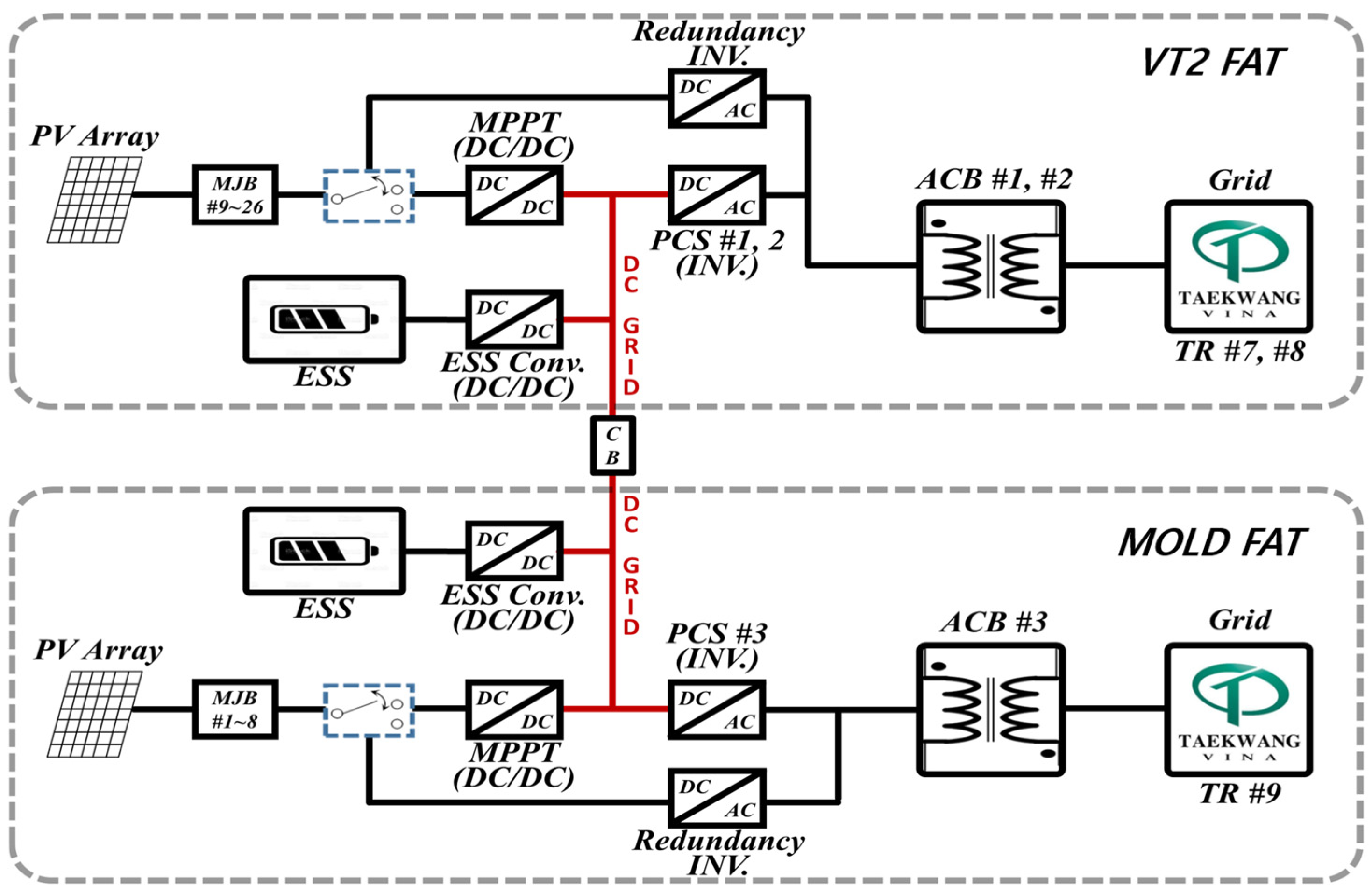
2.1. Overview of the Vietnam Demonstration Site

The demonstration site, located at the Taekwang Vina industrial complex in Dong Nai Province, Vietnam, consists of three distinct facilities: VT2, Mold, and a kindergarten. VT2 is a footwear manufacturing plant that operates many machines and equipment, resulting in high and fluctuating electricity demand. Mold serves as a mold fabrication facility for shoe outer structures, exhibiting a moderately lower and more stable load profile compared to VT2. The kindergarten, designed to accommodate the children of factory employees, has minimal power usage and operates independently from the energy-intensive production sites. Understanding the functional role and load profile of each building provides essential context for the design and operation of the EMS. These contextual differences informed the selection of target buildings for forecasting and ESS scheduling in this study.

As shown in Figure 1, the system operates as a microgrid system integrating various distributed energy resources, including photovoltaic (PV) systems, a combined solar and heat power (CSP/CHP) unit, an energy storage system (ESS), and a centralized Total Operation Control (TOC) center. PV capacity includes 900 kWp on VT2 and 400 kWp on the Mold building. The ESS consists of inverters (1.29 MW), converters (144 kW), and a battery system (720 kWh), supported by MPPT and redundancy inverters. Through the 144 kW rated DC/DC converter, the system allows for a maximum bidirectional power exchange of up to 144 kW between microgrid subsystems, enabling both energy import and export depending on demand and operational strategy. These distributed resources are managed in real time via the TOC to optimize power flow, ensure reliability, and reduce energy costs within the site.

This demonstration site follows a network of microgrids architecture, enabling bidirectional energy exchange between local subsystems. Depending on operational strategies, power can be imported from or exported to other buildings within the industrial complex. This configuration enhances resilience, supports dynamic load balancing, and enables coordinated energy management across distributed assets. Such networked microgrid structures have been shown to improve overall system flexibility and operational efficiency in renewable-integrated environments [17,18,19]. This makes the site an ideal testbed for advanced forecasting and energy optimization techniques in real-world settings.

Additionally, the microgrid architecture includes distributed subsystems deployed at both the VT2 and Mold buildings. As illustrated in Figure 2, each building operates an independent PV-ESS-inverter system interconnected by a DC grid. The VT2 building is equipped with MPPT, ESS converters, and dual PCS inverters feeding into ACB #1 and #2, while the Mold building operates similarly with PCS #3 and ACB #3. Both sites interface with the local Taekwang Vina transformers, enabling grid-tied and isolated microgrid functionality depending on operational strategy.

2.2. Analysis of Meteorological Data in Vietnam

Meteorological variables are generally considered to be among the key factors influencing electric load demand. For this study, temperature, dew point, humidity, and wind speed were selected as input variables for load forecasting [12,13,14].

To determine which weather parameters are most closely correlated with electric load, Pearson correlation analysis was employed. This method quantifies the linear relationship between each meteorological variable and power consumption.

Figure 3 presents the meteorological data collected from Ho Chi Minh City, Vietnam, which consists of hourly observational records. These historical data serve as the foundation for training and validating the forecasting model, providing key input variables such as temperature, dew point, humidity, and wind speed.

The available meteorological dataset includes various features, from which temperature, dew point, humidity, and wind speed were selected for modeling. Figure 4, Figure 5, Figure 6 and Figure 7 visualize the trends and characteristics of these variables—temperature, dew point, humidity, and wind speed—over the data collection period from 10 March to 27 November 2018.

Unlike temperate climate regions in Northeast Asia, which exhibit distinct seasonal variations across spring, summer, fall, and winter, tropical climates in Southeast Asia, including Vietnam, do not show such pronounced seasonal temperature changes. Likewise, other weather features such as humidity and wind speed in tropical regions tend to display weaker seasonal patterns compared to those in temperate zones.

This observation suggests that, unlike in temperate regions, seasonality need not be a major consideration in the model structure for Vietnam. However, since power load is generally known to respond sensitively to heating and cooling needs driven by temperature, a strong correlation between load and temperature is expected.

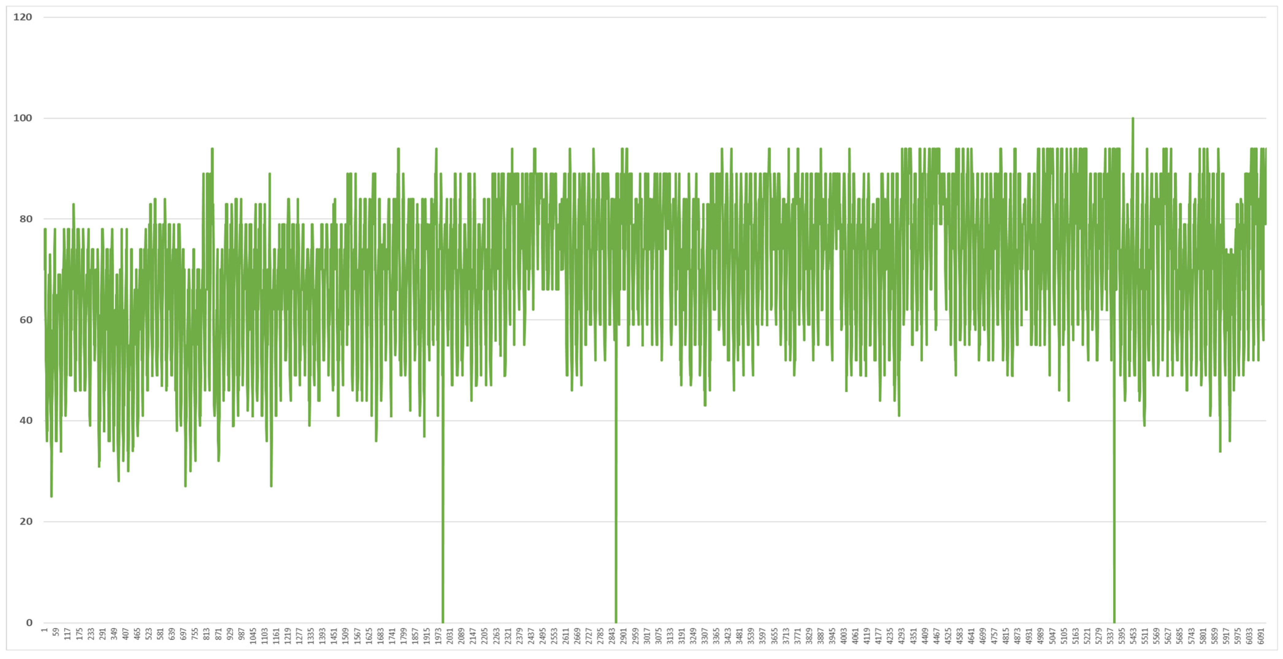
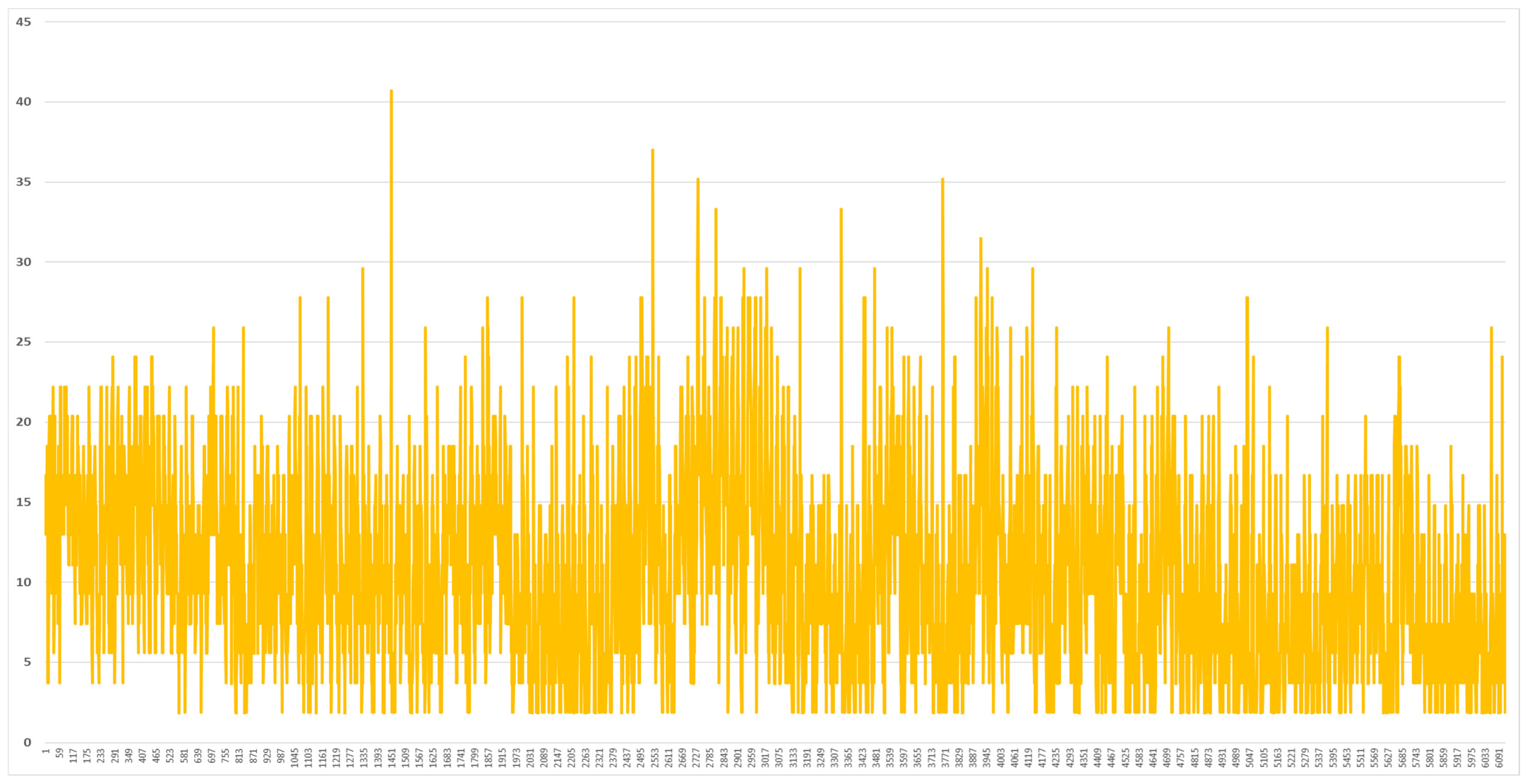
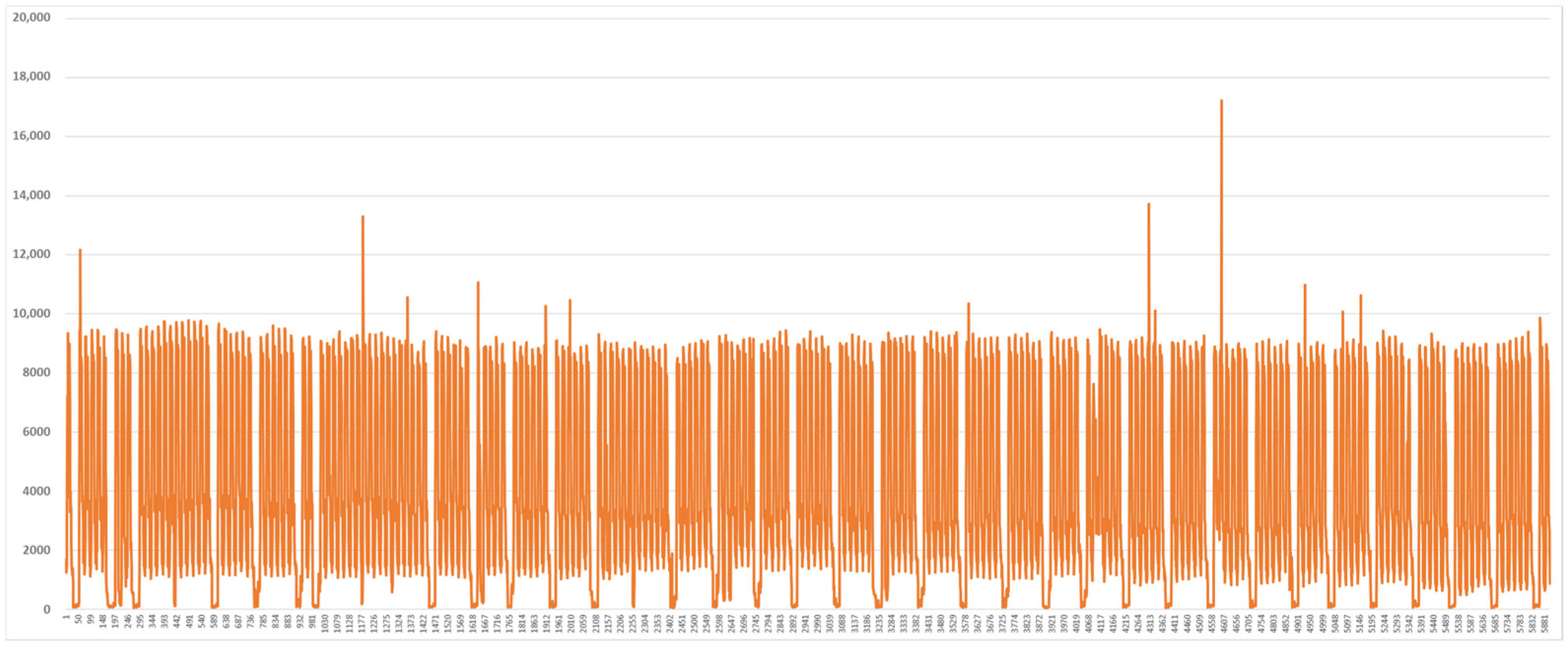
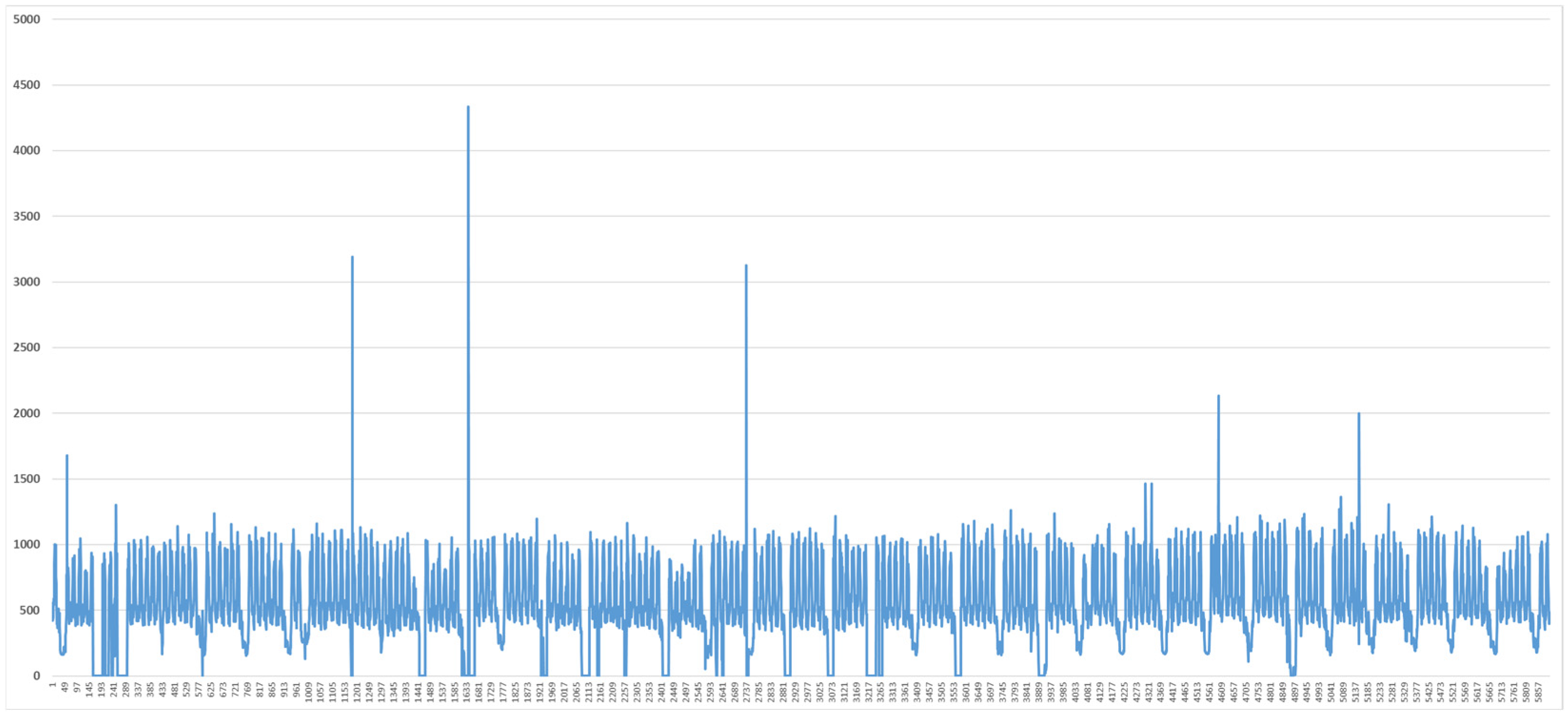
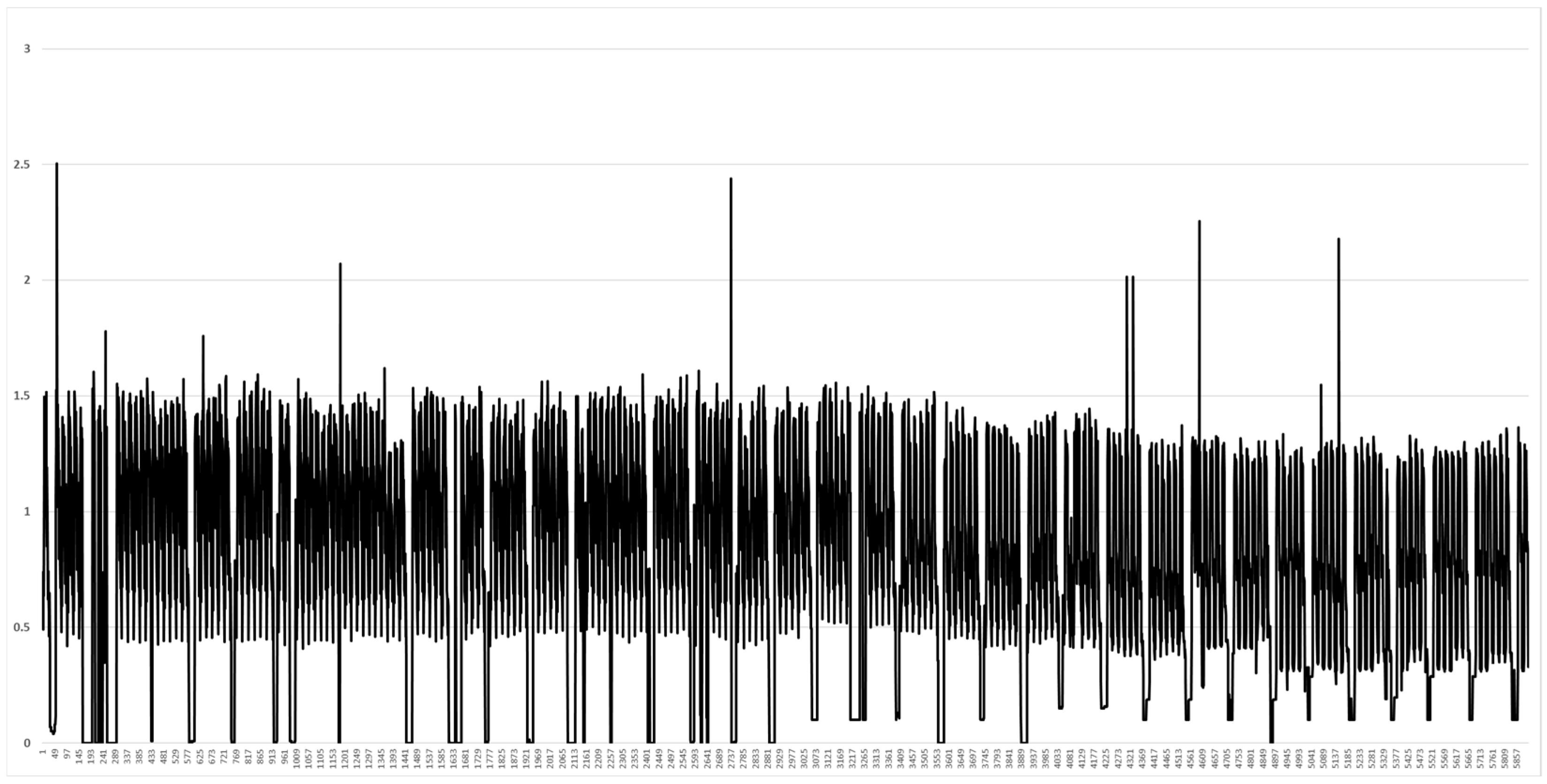
2.3. Analysis of Load Data in the Vietnam Demonstration Site

To further illustrate the load behavior at each site, representative load profiles were visualized. Figure 8, Figure 9 and Figure 10 illustrate the hourly load patterns of these buildings—VT2, Mold, and Kindergarten—for the period between 10 March and 27 November 2018. While some data points show abrupt spikes or drops in load, overall, the load tends to be higher during the winter season (December to March) and the summer season (July to September) compared to other periods.

Additionally, a broader review of historical load patterns reveals a general increasing trend in power consumption from 2015 to 2017, suggesting long-term load growth at the site. The electric load data collected from the Vietnam demonstration factory site was obtained from three key buildings within the site—VT2, Mold, and Kindergarten—each representing different usage patterns and operational characteristics. By analyzing historical load trends, we were able to identify temporal patterns and assess variations between weekdays and weekends. This insight formed the basis for training individual ANN models per building to optimize forecast accuracy under localized conditions [20].

While some data points show abrupt spikes or drops in load, overall, the load tends to be higher during the winter season (December to March) and the summer season (July to September) compared to other periods.

Additionally, a broader review of historical load patterns reveals a general increasing trend in power consumption from 2015 to 2017, suggesting long-term load growth at the site. The electric load data were collected from the Vietnam demonstration factory site. Load data were obtained from three key buildings within the site—VT2, Mold, and Kindergarten—each representing different usage patterns and operational characteristics. By analyzing historical load trends, we were able to identify temporal patterns and assess variations between weekdays and weekends. This insight formed the basis for training individual ANN models per building to optimize forecast accuracy under localized conditions.

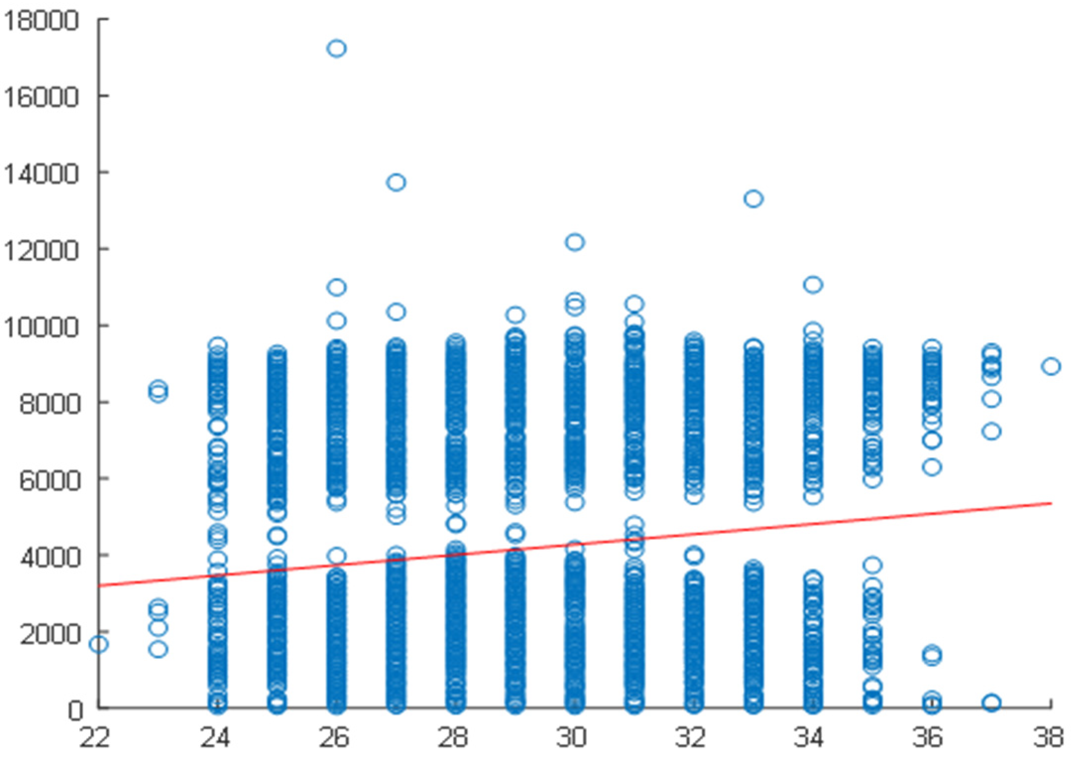
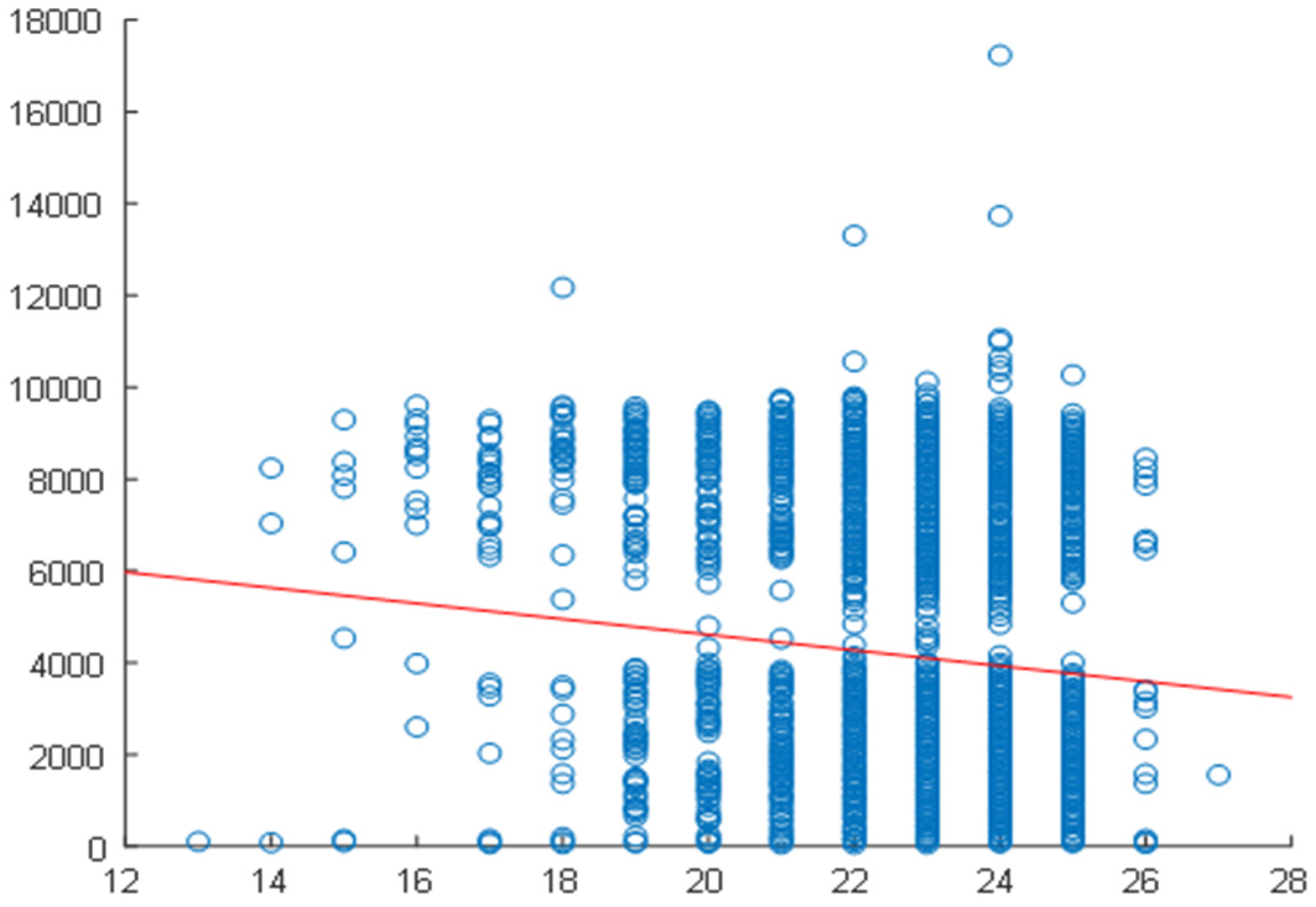
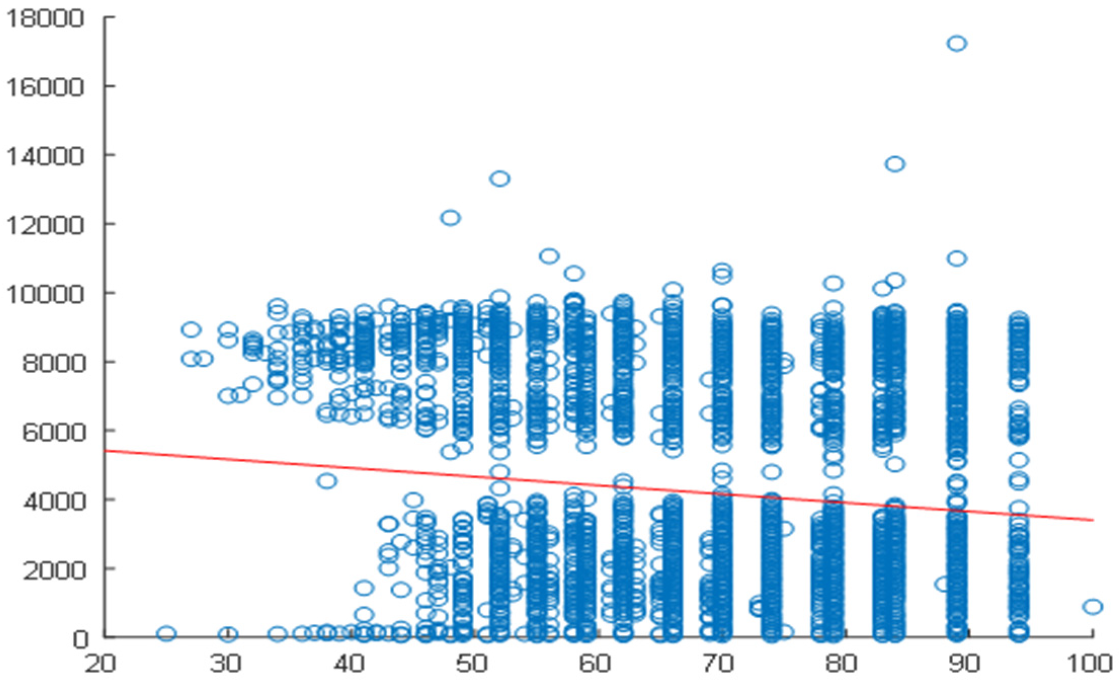
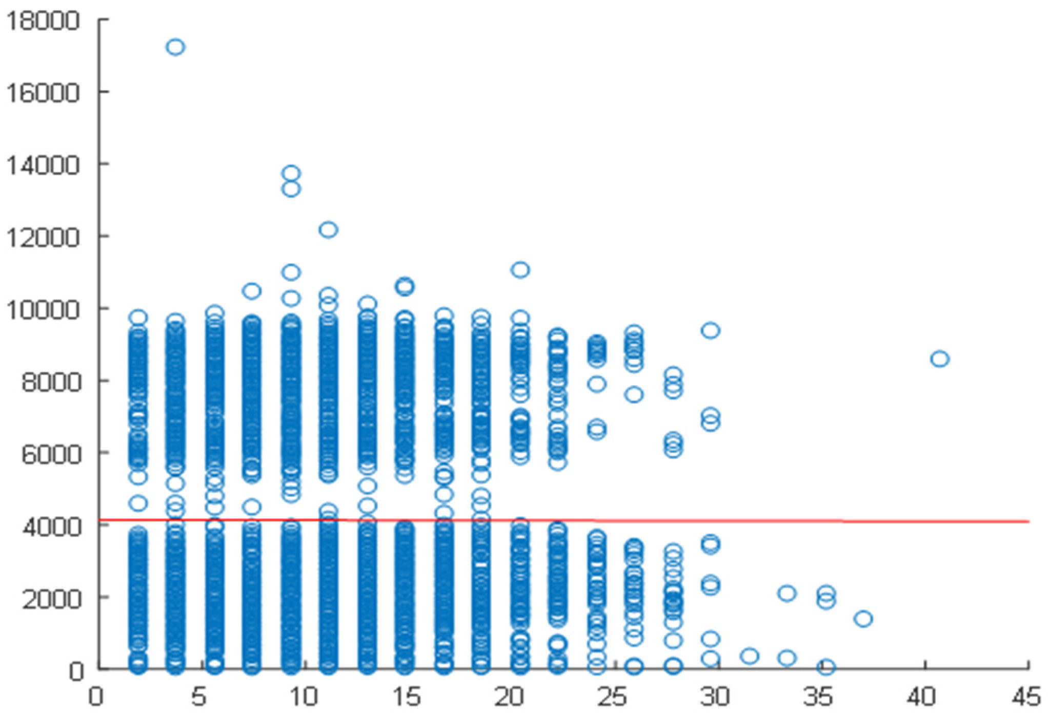
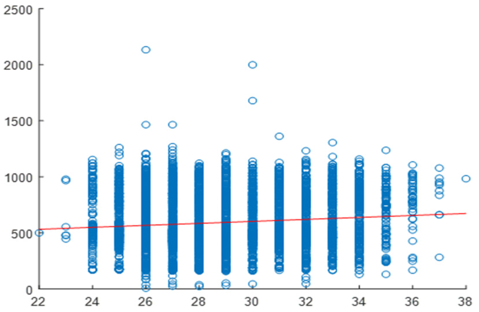
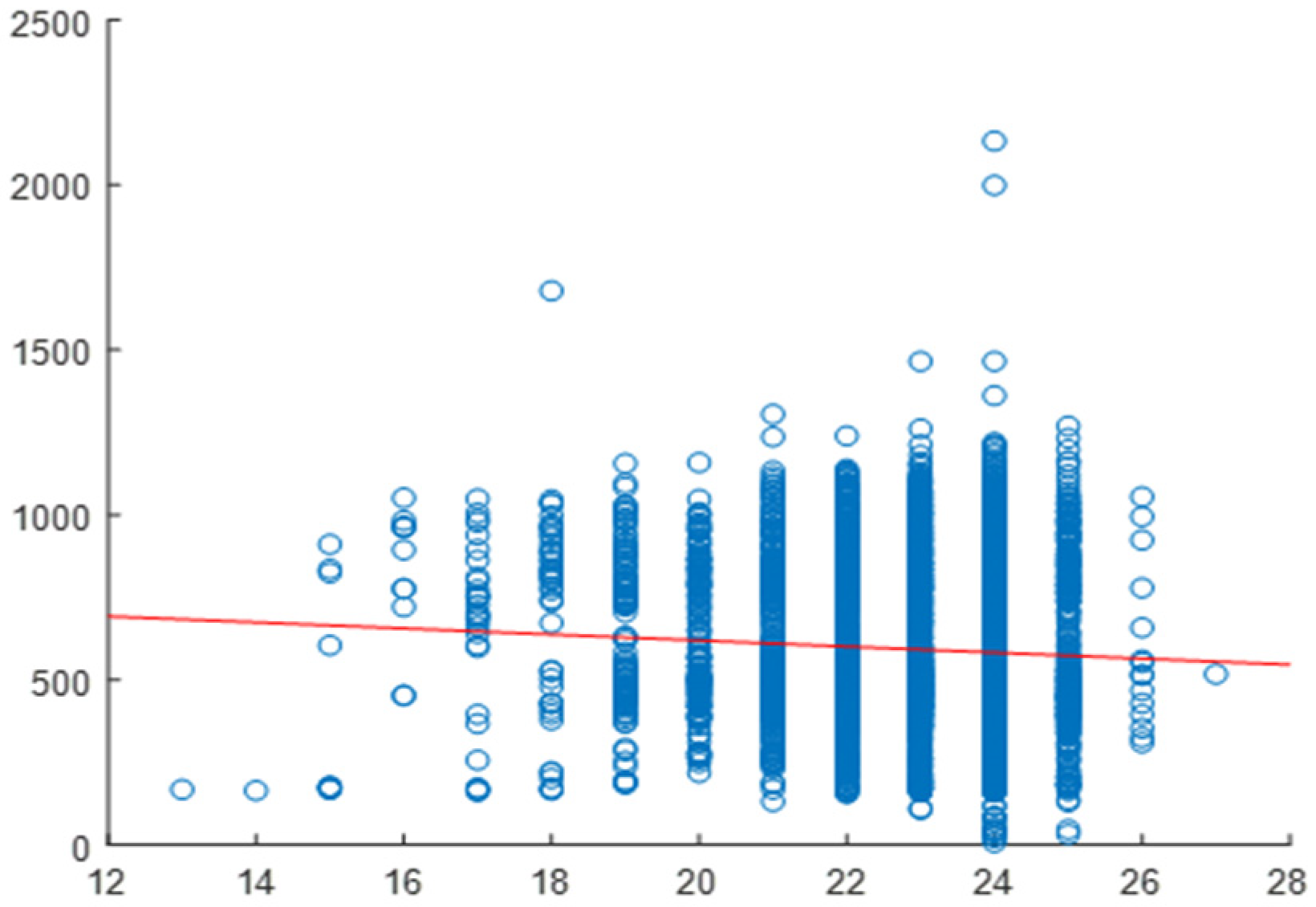
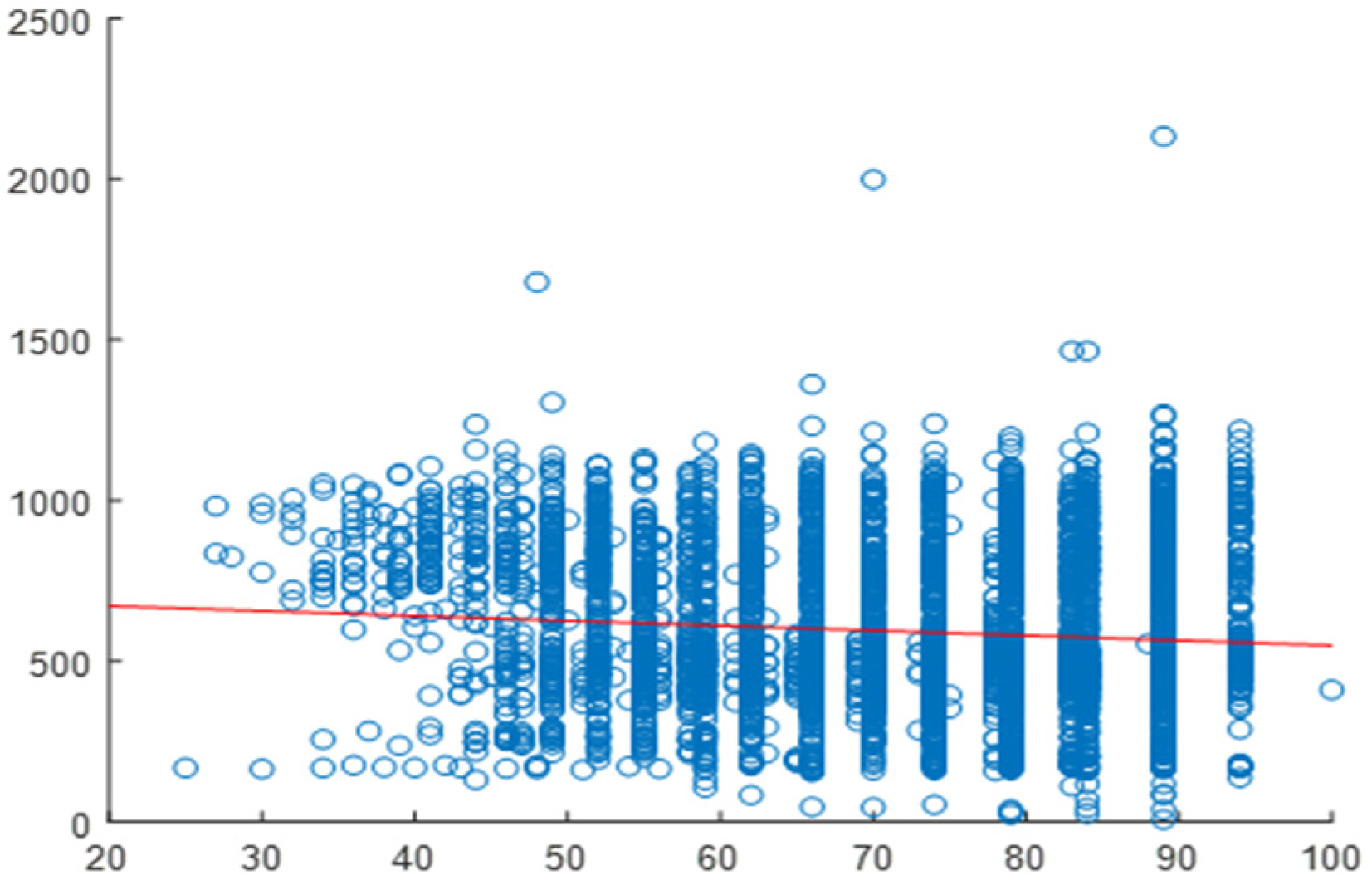
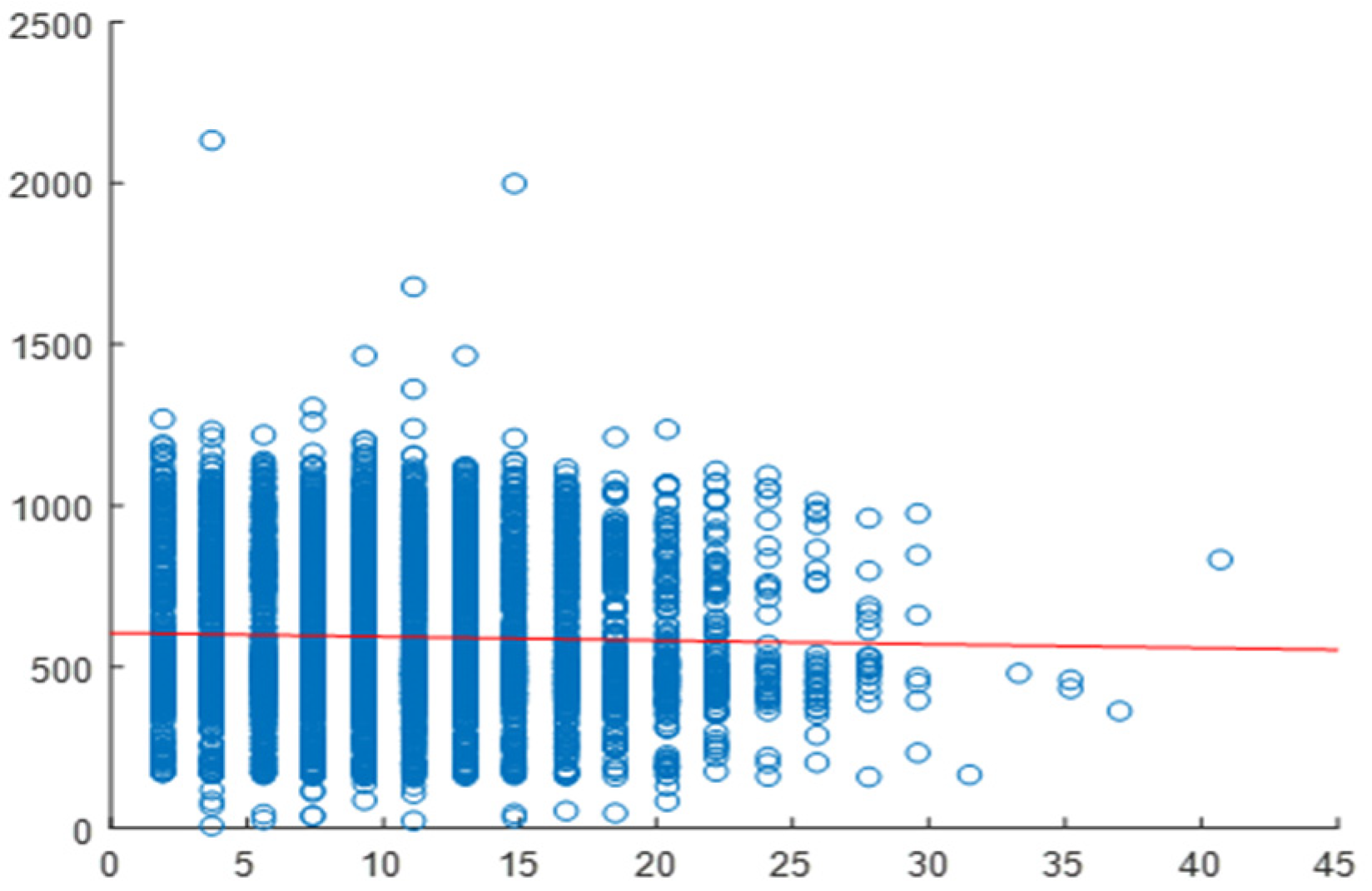
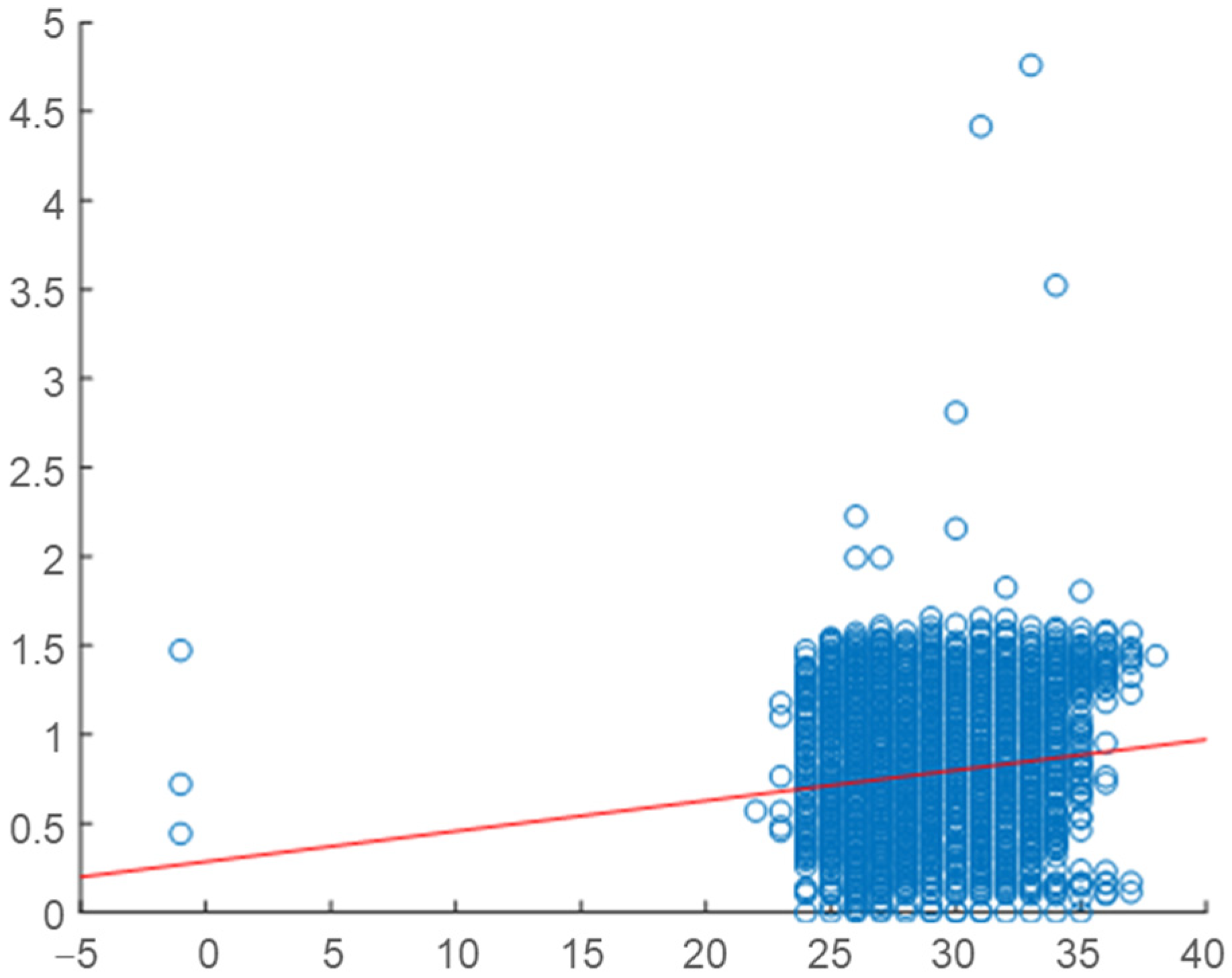
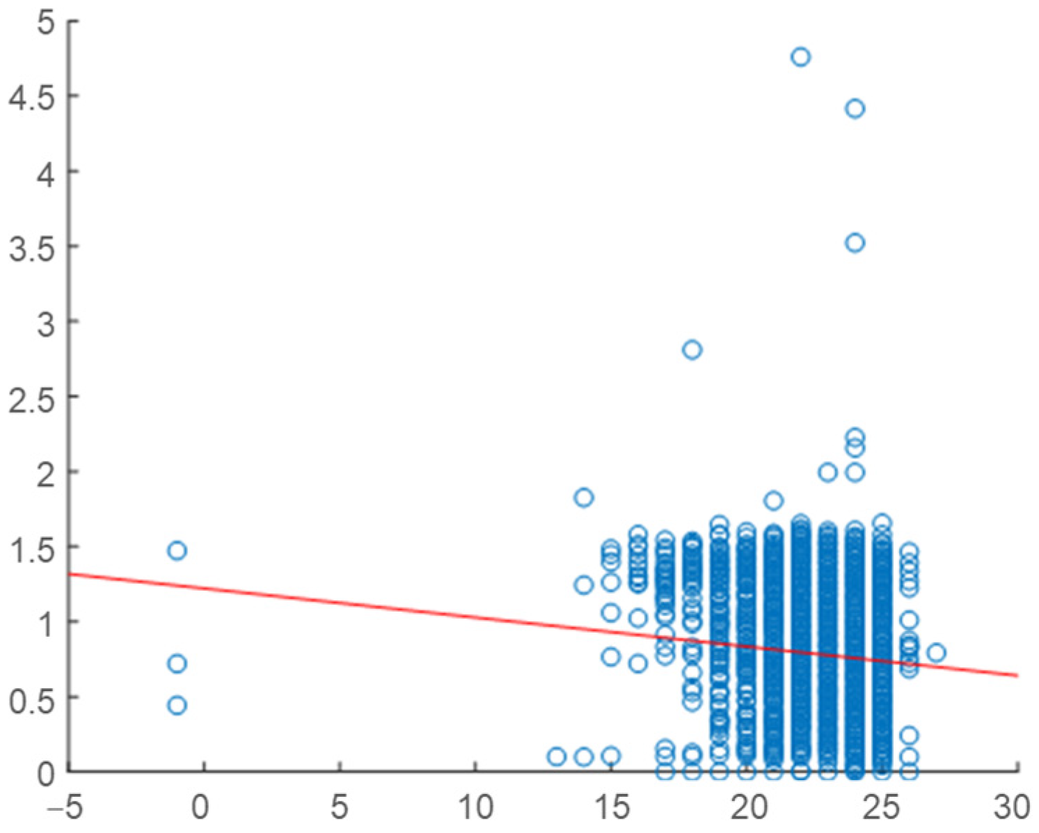
2.4. Correlation Analysis

Correlation analysis in this study is supported by the use of the Pearson correlation coefficient, which quantitatively evaluates the degree of linear relationship between a meteorological variable and electric load. The formula used is as follows:

$$R_m={\displaystyle \frac{n\sum X_{m}Y-\left(\sum X_m\right)\left(\sum Y\right)}{\sqrt{\left(n\sum X_m^2-{\left(\sum X_m\right)}^2\right)\left(n\sum Y^2-{\left(\sum Y\right)}^2\right)}}}$$

(1)

where

$R_m$: Pearson correlation coefficient between meteorological variable $X_m$ and power load $Y$;

$n$: number of data points;

$X_m$: meteorological data (e.g., temperature and humidity);

$Y$: power consumption data.

Interpretation:

$R_m=1$: perfect positive linear relationship;

$R_m=-1$: perfect negative linear relationship;

$R_m=0$: no linear relationship.

This formula is a standard statistical tool that helps in determining the strength and direction of a linear relationship between two continuous variables. It forms the basis of variable selection in our forecasting model.

Correlation analysis is a statistical method used to assess the linear relationship between two variables. The correlation coefficient quantifies this relationship, where a value close to 1 or −1 indicates strong positive or negative correlation, respectively, and values near 0 suggest little to no linear correlation.

In this study, Pearson correlation coefficient was used to evaluate the relationship between meteorological variables (temperature, dew point, humidity, and wind speed) and power consumption. This method was applied over the entire period of data collection (10 March to 27 November 2018) to identify which variables have the strongest association with load patterns.

Visualizations using scatter plots were also generated to provide an intuitive understanding of these relationships. To enhance this analysis, we visualized the relationship between VT2 building load and meteorological variables over the entire data collection period (10 March to 27 November 2018), as shown in Figure 11, Figure 12, Figure 13 and Figure 14. The scatter plots below illustrate these correlations clearly, allowing us to visually interpret the strength and direction of each variable’s influence on power demand. The results show that, while temperature and dew point exhibit weak linear correlations with load, humidity and wind speed have even weaker or negligible associations, as quantified in the following figures.

Temperature exhibits a weak positive linear correlation with power load, indicated by a Pearson correlation coefficient of 0.1194. Dew point also shows a very weak negative linear relationship with load, with a coefficient of −0.0828. Similarly, humidity demonstrates a weak negative correlation of −0.1077 with load. In contrast, wind speed displays virtually no linear association with load, as shown by a near-zero correlation coefficient of −0.0020.

Temperature and power load for the Mold building exhibit a weak linear correlation, with a Pearson correlation coefficient of 0.1073. Dew point and load show a very weak negative linear correlation, with a coefficient of −0.0598. Humidity shows a similarly weak negative relationship with load, with a coefficient of −0.0906. Wind speed demonstrates virtually no linear correlation with Mold load, as shown by a correlation coefficient of −0.0279. These relationships are illustrated in Figure 15, Figure 16, Figure 17 and Figure 18.

Kindergarten building load data show similar patterns. Temperature shows a weak positive linear relationship with load, with a Pearson coefficient of 0.1149. Dew point and load have a very weak negative correlation of −0.0729, while humidity correlates negatively with a coefficient of −0.1104. Wind speed shows a very weak positive correlation with kindergarten load, with a coefficient of 0.0548. These relationships are illustrated in Figure 19, Figure 20, Figure 21 and Figure 22.

The results above differ somewhat from the expectations formed during the meteorological data analysis in Section 2.1. It is commonly understood that electric load is highly sensitive to temperature due to heating and cooling demands, which would suggest a strong correlation between temperature and power load. However, the observed Pearson correlation coefficients indicate that the relationship is not significantly strong. Similar weak or negligible correlations were found for other meteorological variables as well.

The weak overall correlation between temperature and electric load observed in this study can primarily be attributed to the non-linear and intermittent nature of weather influences under Vietnam’s tropical climate. In such environments, sudden changes in humidity, solar radiation, or wind may affect energy usage in brief, irregular patterns that are not consistently captured over long-term aggregations. Additionally, the load characteristics of the studied buildings reflect the operational realities of industrial footwear manufacturing for globally recognized consumer brands. As original equipment manufacturing (OEM) sites, their production schedules tend to follow market-driven demand and fashion cycles rather than seasonal climate changes, further decoupling electric load from meteorological conditions.

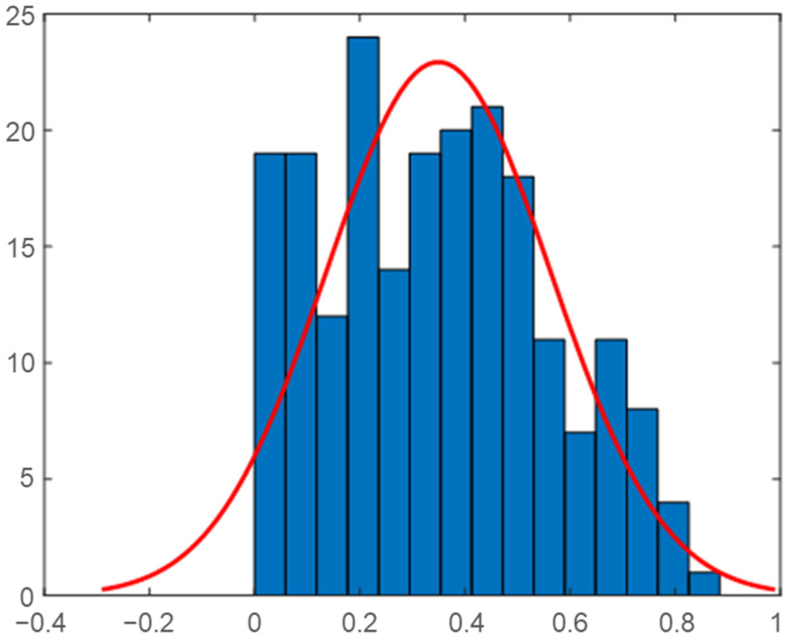
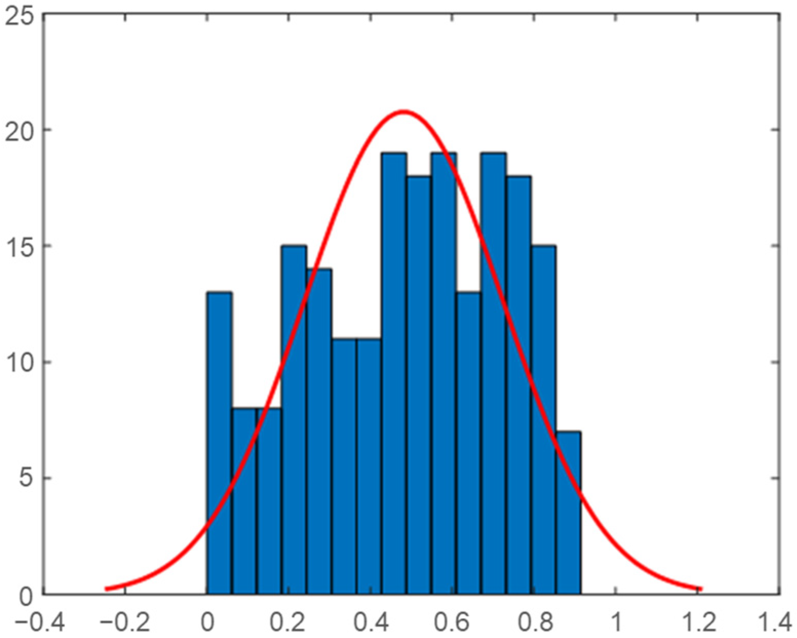
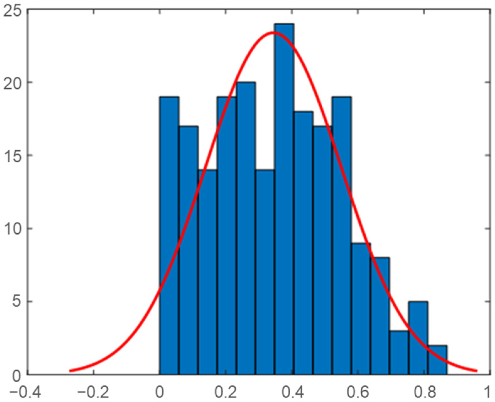
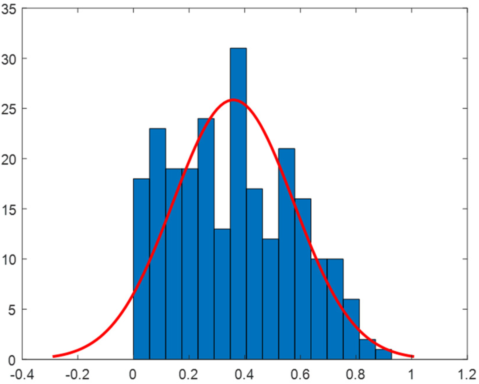
2.5. Daily Correlation Trend Analysis

While the previous section analyzed the overall correlation between meteorological variables and power load across the entire dataset, this section presents the distribution of Pearson correlation coefficients calculated on a daily basis. Given that power forecasting is often performed over 24 h periods, understanding the day-to-day variation in correlation can provide more granular insight into the strength of relationships over time.

Histograms were generated to visualize the daily correlation coefficient distributions for each building (VT2, Mold, and Kindergarten) across the four meteorological variables: temperature, dew point, humidity, and wind speed. These distributions offer a more nuanced view of the dynamic relationships between weather conditions and power demand, which can vary significantly based on operational schedules, weather fluctuations, and building use patterns.

For the VT2 building, Figure 23, Figure 24, Figure 25 and Figure 26 present the histograms showing the distribution of daily Pearson correlation coefficients between power load and each meteorological variable.

Temperature and power load demonstrate a strong linear relationship, with most daily Pearson correlation values ranging between 0.6 and 0.8. This suggests a consistent and strong dependency between temperature and load throughout each day. Dew point shows a moderate relationship with daily load values, where the majority of correlation coefficients fall between 0.3 and 0.5, indicating a weaker but present linear trend.

Humidity also reflects a strong correlation pattern, with values similarly clustered within the 0.6 to 0.8 range. Wind speed, on the other hand, exhibits a notably weaker correlation, with most values distributed between 0 and 0.4, suggesting limited influence on the daily power load.

For the Mold building, Figure 27, Figure 28, Figure 29 and Figure 30 illustrate the daily Pearson correlation coefficient distributions for each meteorological factor.

Temperature and power load show a moderately strong linear relationship, with most daily correlation values falling within the 0.4 to 0.6 range. Dew point also displays a moderate correlation, where daily coefficients typically range from 0.3 to 0.5, indicating a consistent linear association across days.

Humidity demonstrates a stronger linear relationship with load, with correlation values predominantly between 0.6 and 0.8. In contrast, wind speed correlations are generally weaker, with daily coefficients mostly distributed between 0 and 0.4, suggesting minimal impact on daily load patterns.

For the kindergarten building, Figure 31, Figure 32, Figure 33 and Figure 34 illustrate the histograms representing the distribution of daily Pearson correlation coefficients with respect to the selected meteorological factors.

Temperature and load correlations are consistently strong, with values mainly distributed between 0.4 and 0.8. This suggests a reliable and moderately strong relationship throughout the day. Dew point shows a weaker but still notable linear association, with daily correlation coefficients ranging between 0.2 and 0.5.

Humidity demonstrates a strong linear correlation with load, as coefficients are primarily within the 0.6 to 0.8 range. Wind speed again shows only a weak relationship, with most correlation values falling between 0 and 0.4.

The daily correlation histograms in Figure 23, Figure 24, Figure 25, Figure 26, Figure 27, Figure 28, Figure 29, Figure 30, Figure 31, Figure 32, Figure 33 and Figure 34 reveal a different trend from the aggregated analysis. For example, in the VT2 building, daily correlations between temperature and load frequently range from 0.6 to 0.8, suggesting a strong and consistent relationship at the intra-day level. This indicates that HVAC usage may spike during specific temperature conditions or time windows (e.g., mid-day peak hours), even in the absence of pronounced seasonal changes. Such transient behaviors are masked in the overall analysis due to temporal averaging. This reinforces the importance of day-level analysis when forecasting load in climates with minimal seasonality but high daily variability.

The following

Table 1. Summary of correlation analysis results.

Building	Variable	Overall Correlation	Daily Correlation Range	Strength of Relationship
VT2	Temperature	0.1194	0.6–0.8	Strong
	Dew Point	−0.0828	0.3–0.5	Moderate
	Humidity	−0.1077	0.6–0.8	Strong
	Wind Speed	−0.002	0–0.4	Weak
Mold	Temperature	0.1073	0.4–0.6	Moderate
	Dew Point	−0.0598	0.3–0.5	Moderate
	Humidity	−0.0906	0.6–0.8	Strong
	Wind Speed	−0.0279	0–0.4	Weak
Kindergarten	Temperature	0.1149	0.4–0.8	Moderate to Strong
	Dew Point	−0.0729	0.2–0.5	Weak to Moderate
	Humidity	−0.1104	0.6–0.8	Strong
	Wind Speed	0.0548	0–0.4	Weak

summarizes the key findings from Section 2.4 and Section 2.5, highlighting both overall and daily Pearson correlation coefficient trends between meteorological variables and electric load for each of the three buildings.

The observed discrepancy between overall and daily correlation coefficients can be attributed to several interacting factors. Daily operational schedules, such as work shifts and equipment usage in VT2 and Mold buildings, vary significantly across weekdays and weekends, causing fluctuations in hourly load patterns. In addition, transient weather conditions—such as sudden humidity surges or temperature drops—may influence short-term cooling or ventilation demands. Each building’s unique usage profile, including the kindergarten’s non-production-based occupancy, also contributes to the varying sensitivity of load to meteorological changes. These factors, when combined, lead to non-linear and temporally dynamic relationships between weather and load, which are better captured in daily correlation analyses than in aggregated values.

3. Methodology

This section outlines the structure and implementation of the load forecasting model developed in this study. The model is based on artificial neural networks (ANNs), which are capable of capturing complex and non-linear relationships between weather variables and electric load. By employing building-specific models and incorporating multiple weather variables, the proposed methodology aims to enhance short-term forecasting accuracy in industrial microgrid environments.

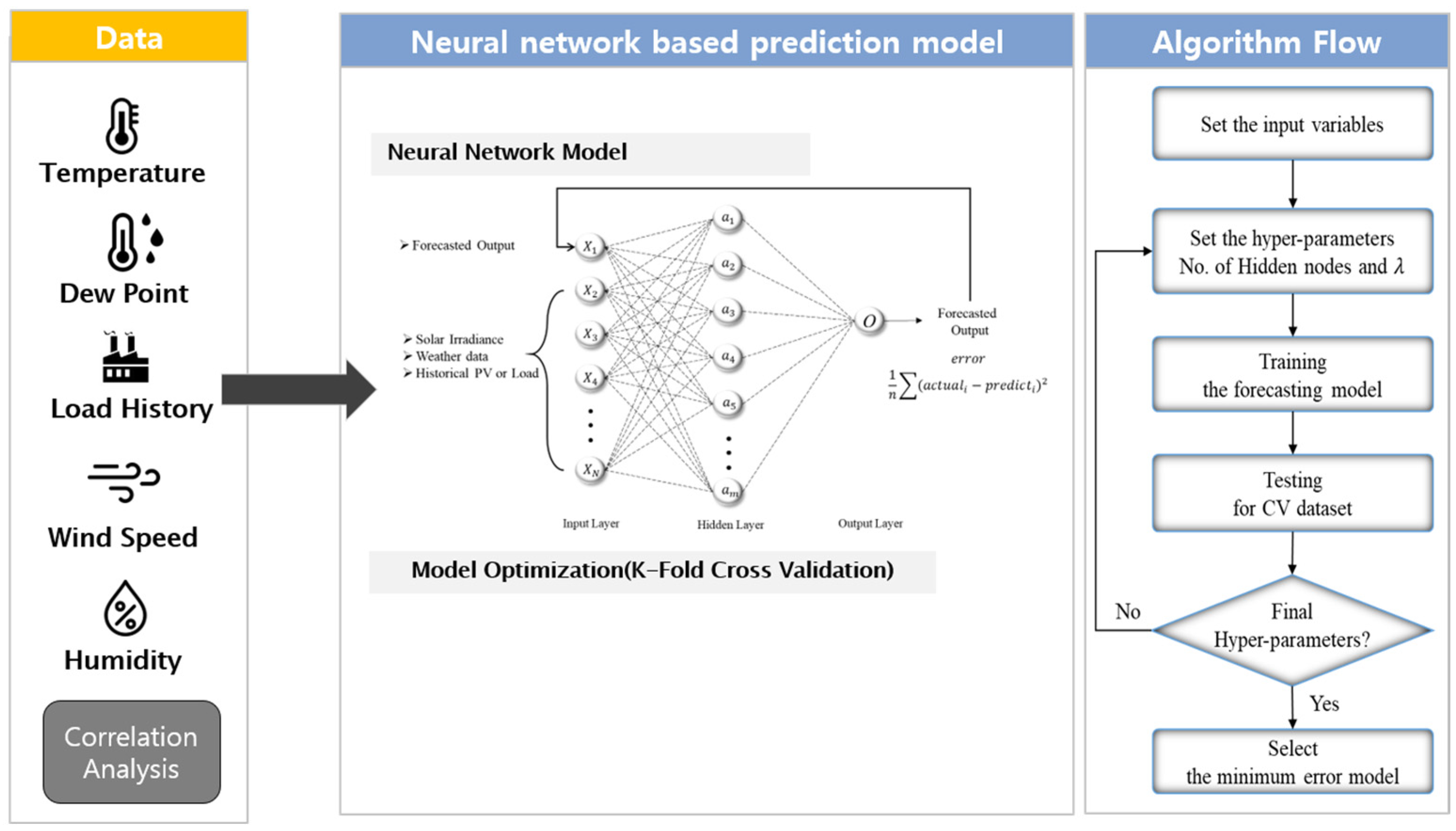
3.1. ANN Model Design

The output of the Softplus activation function used in the hidden layers is defined as:

$$f\left(x\right)=\ln \left(1+e^x\right)$$

(2)

This activation function is continuous and differentiable, which makes it well-suited for gradient-based optimization. Unlike the ReLU function that outputs zero for negative inputs, the Softplus function maintains a smooth gradient for all input values, enabling more stable learning during training. It serves as a smooth approximation to the ReLU function while avoiding issues related to gradient vanishing in deeper layers.

$$\begin{array}{c}{h}^{\left(1\right)}=\ln \left(1+e^{W^{\left(1\right)}x+b^{\left(1\right)}}\right)\\ h^{\left(2\right)}=\ln \left(1+e^{W^{\left(2\right)}{h}^{\left(1\right)}+b^{\left(2\right)}}\right)\\ \widehat{\mathit{y}}=W^{\left(3\right)}{h}^{\left(2\right)}+b^{\left(3\right)}\end{array}$$

(3)

This equation describes the sequence of transformations applied to the input data through each layer of the neural network. The first hidden layer computes a non-linear mapping of the input weather variables, enabling the model to capture direct influences on load. The second hidden layer processes the output of the first to uncover higher-order dependencies and interactions among the features. The output layer then generates the final predicted load value. This architecture allows the model to approximate highly complex, non-linear relationships in the data that traditional models may fail to capture, making it particularly suitable for energy forecasting in diverse environmental conditions.

This equation illustrates the full forward propagation process of the ANN used in this study. It includes two hidden layers, each applying the Softplus activation function, and a linear output layer that produces the final power load prediction.

This function allows the network to handle non-linearity while avoiding issues related to vanishing gradients commonly seen in sigmoid or tanh functions.

The proposed forecasting model utilizes a multi-layer perceptron (MLP) architecture. The input layer receives four normalized weather variables: temperature, dew point, humidity, and wind speed. The model is structured to produce hourly electric load forecasts for a 24 h horizon, enabling day-ahead prediction of power demand.

Each ANN consists of one input layer, two hidden layers, and one output layer. The hidden layers use the Softplus activation function, which was selected for its ability to handle non-linearities while maintaining smooth gradients for optimization. The output layer generates the predicted hourly load values. These two hidden layers enable the network to capture more complex non-linear relationships between inputs and outputs. The first hidden layer identifies basic interaction patterns among weather variables, while the second layer builds upon these to learn higher-level abstractions. This multi-layered structure increases the model’s capacity to approximate intricate patterns in load behavior, improving forecast accuracy over single-layer designs.

This model is particularly suitable for capturing non-linear dependencies between weather variables and load patterns. Given the frequent short-term fluctuations in tropical climates like Vietnam, the ANN structure helps maintain prediction robustness even under abrupt weather shifts or irregular factory operation schedules, which are difficult to handle with traditional linear approaches.

3.2. Model Training and Evaluation

The loss function minimized during training is the Mean Squared Error (MSE), expressed as:

$$\mathrm{M}\mathrm{S}\mathrm{E}=\left({\displaystyle \frac{1}{\mathrm{n}}}\right) \mathrm{\ast } \Sigma {\left({\mathrm{y}}_{\mathrm{i}}-{\mathrm{ŷ}}_{\mathrm{i}}\right)}^2$$

(4)

where y_i is the actual load and ŷ_i is the predicted load for instance i.

The forecasting performance was evaluated using the Mean Absolute Percentage Error (MAPE), calculated as:

$$\mathrm{M}\mathrm{A}\mathrm{P}\mathrm{E}=\left({\displaystyle \frac{100}{\mathrm{n}}}\right) \mathrm{\ast } \Sigma \left({\displaystyle \frac{\left|{\mathrm{y}}_{\mathrm{i}}-{\mathrm{ŷ}}_{\mathrm{i}}\right|}{{\mathrm{y}}_{\mathrm{i}}}}\right)$$

(5)

This metric quantifies the accuracy of the forecasts as a percentage of the actual load.

The model was trained using historical weather data and corresponding load measurements for the VT2, Mold, and Kindergarten buildings. Data was split into training and validation sets with a typical 80:20 ratio. Mean Squared Error (MSE) was used as the loss function, and model performance was evaluated using the Mean Absolute Percentage Error (MAPE) metric.

The input data was standardized to have zero mean and unit variance to enhance learning efficiency and convergence. Model training was conducted independently for each building to account for their different load characteristics and operational profiles.

The ANN architecture consists of an input layer, two hidden layers with 16 and 8 neurons, respectively, and an output layer. The Softplus activation function is applied to the hidden layers, and a linear activation is used in the output. The network was trained using the Adam optimizer with a learning rate of 0.001. The batch size was set to 32, and training was conducted over 100 epochs. These parameters were selected based on preliminary experiments to balance convergence speed and prediction accuracy. Model performance was monitored using validation loss under K-fold cross-validation.

3.3. Forecasting Approach

Separate ANN models were trained for each building using the respective historical data. Forecasts were performed on a day-ahead basis, with the model generating 24 hourly load predictions at once. Figure 35 illustrates the end-to-end architecture and flow of the ANN-based forecasting model developed in this study. The model receives multiple meteorological variables (temperature, dew point, humidity, and wind speed) along with load history as inputs. The forecasting engine consists of a multi-layer perceptron with two hidden layers using the Softplus activation function. To ensure generalization, the model undergoes K-fold cross-validation, where each fold is used once for validation while the remaining folds are used for training. Hyperparameters, such as the number of hidden nodes and regularization coefficient, are tuned based on the average validation error. This approach enables the selection of an ANN configuration that minimizes generalization error and enhances prediction reliability. By tailoring the ANN model to each building’s data, the method improves localized forecasting accuracy, capturing site-specific behaviors and weather sensitivities.

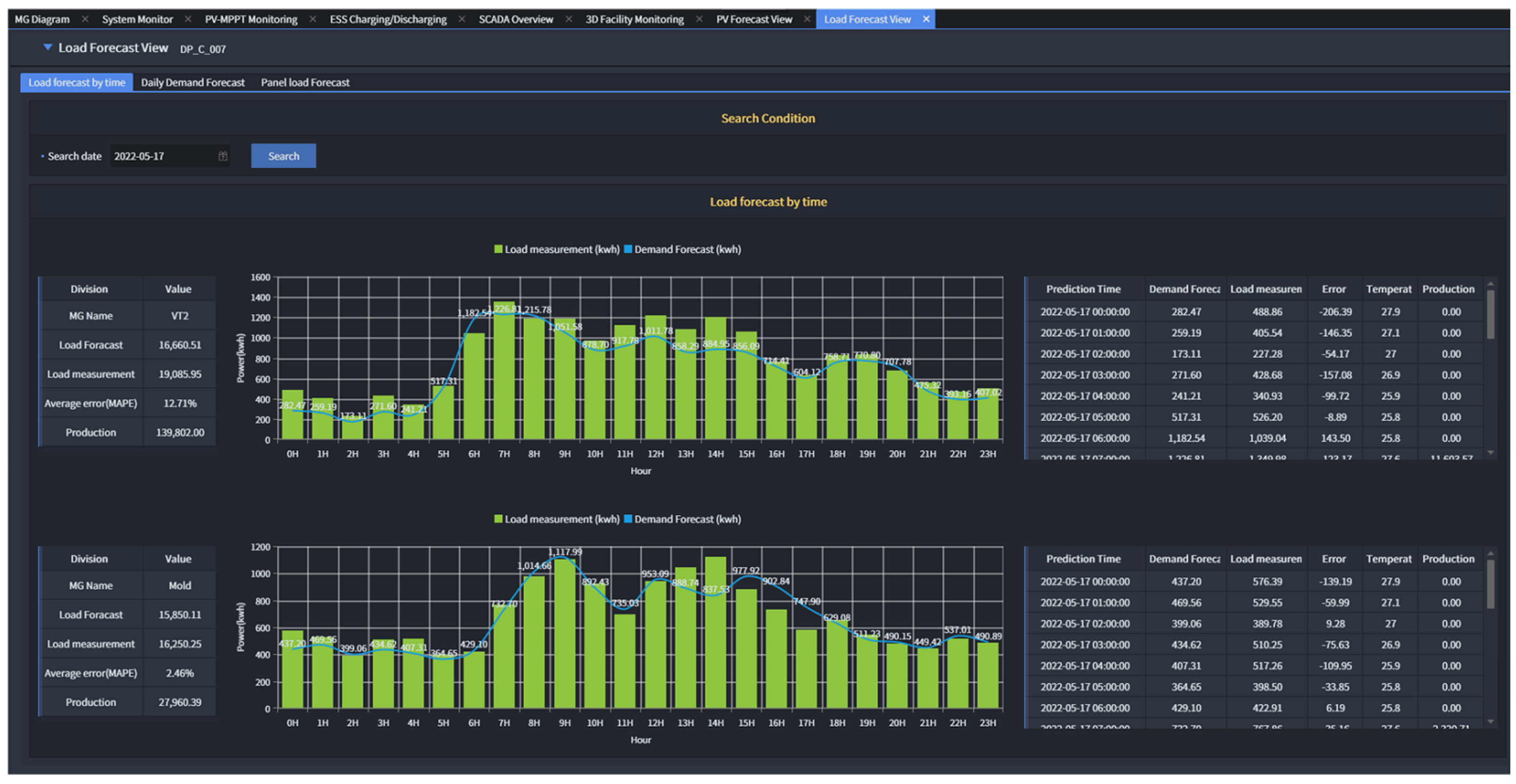
4. Results and Performance Evaluation

This section presents the results of the electric load forecasting using the proposed ANN-based models for the VT2, Mold, and Kindergarten buildings. Each building’s model was evaluated based on its ability to accurately predict 24 h ahead load values using meteorological inputs.

The models demonstrated consistent and reliable prediction performance across all three buildings. For each case, the ANN model captured the daily load pattern with sufficient accuracy, despite differing operational schedules and sensitivities to meteorological inputs. As shown in

Table 2. Forecasting accuracy for each building.

Building	MAPE (%)
VT2	10.2
Mold	8.8
Kindergarten	10.6

, MAPE scores ranged from 8.8% to 10.6%, suggesting effective learning and generalization by the ANN model.

To further validate prediction performance, Figure 36, Figure 37 and Figure 38 compare actual and predicted load values over a representative day for each building. In the figures, the actual load is shown in blue, while the predicted load is illustrated in red. Among the three buildings, both VT2 and Mold are factory buildings, while the kindergarten is an educational facility. VT2 has the highest average power consumption, whereas Mold represents one of the lower-load industrial sites. Interestingly, despite its lower total load, the Mold building shows better prediction alignment. This suggests that stable and predictable load behavior, rather than total consumption, may play a more critical role in achieving accurate forecasts. The results show that the ANN model effectively captures both peak and off-peak load trends, even during times of abrupt changes. This is especially evident in the Mold building, where the ANN demonstrates higher precision, likely due to consistent usage and more predictable weather–load interaction.

In contrast, VT2 and Kindergarten buildings showed slightly higher MAPE values, possibly due to variable schedules or complex usage behaviors not directly explained by the four weather variables used. Nevertheless, the visual alignment of predicted and observed values in these figures supports the model’s robustness.

Overall, these findings suggest that the proposed ANN model is well-suited for site-specific energy demand forecasting and has the potential to support microgrid optimization and operational planning.

5. EMS Operation Strategy Based on Load Forecasting

5.1. Forecast-Aided Load Scheduling

Although load forecasting was conducted for three sites—VT2, Mold, and a kindergarten—the EMS operation and ESS scheduling in this study focused only on the VT2 and Mold buildings. This is because the kindergarten’s electric load was significantly smaller and less variable compared to the industrial facilities, rendering it unnecessary to include in the economic scheduling and control framework. However, its load patterns were still considered as part of the overall demand profile for monitoring purposes.

Figure 39 and Figure 40 illustrates the forecasting system, which is built upon the integration of local climate data, historical load patterns, and facility schedule information. As shown in the diagram, key meteorological parameters such as temperature, dew point, humidity, and wind speed, along with factory-specific load history, are processed through Pearson correlation analysis to identify significant relationships. This data is then fed into a multi-layer artificial neural network (ANN) for prediction, the integration of local climate data, historical load patterns, and facility schedule information.

To ensure reliability, a K-fold cross-validation approach is employed during model training, verifying performance across multiple data splits. The resulting ANN model can then deliver a 24 h ahead load forecast for each building.

This forecast supports real-time scheduling for industrial microgrids. It enables the EMS to proactively plan charging and discharging of energy storage, schedule surplus power exchanges, and maintain operational efficiency even under fluctuating load conditions. The model achieves a mean absolute percentage error (MAPE) within 12%, as shown in the following illustration.

This image shows actual versus predicted electric load values for the VT2 and Mold buildings on 17 May 2022. The upper chart corresponds to VT2, where an MAPE of 12.71% was observed, and the lower chart shows Mold with an MAPE of just 2.46%. Each bar represents measured load (green), while the blue line denotes the forecasted demand. The error values and temperature inputs are tabulated on the right side. The higher accuracy in Mold likely reflects a more consistent load pattern compared to VT2’s operational fluctuations.

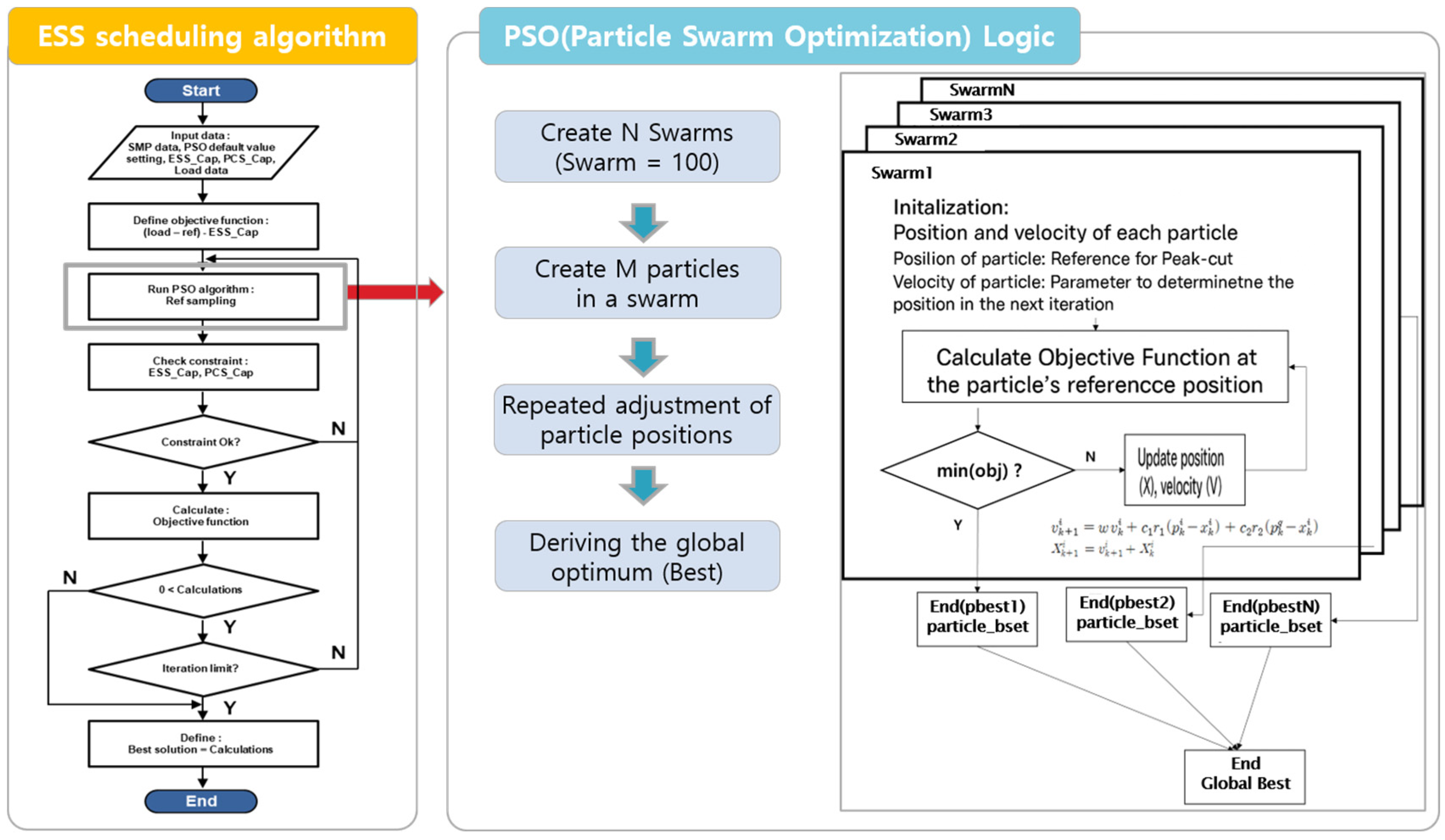
5.2. Economic Operation with PSO Algorithm

The proposed Energy Management System (EMS) integrates a Particle Swarm Optimization (PSO) algorithm to generate optimal charge and discharge schedules for each building’s Energy Storage System (ESS). This optimization minimizes operational cost while satisfying system constraints and responding to forecasted load conditions.

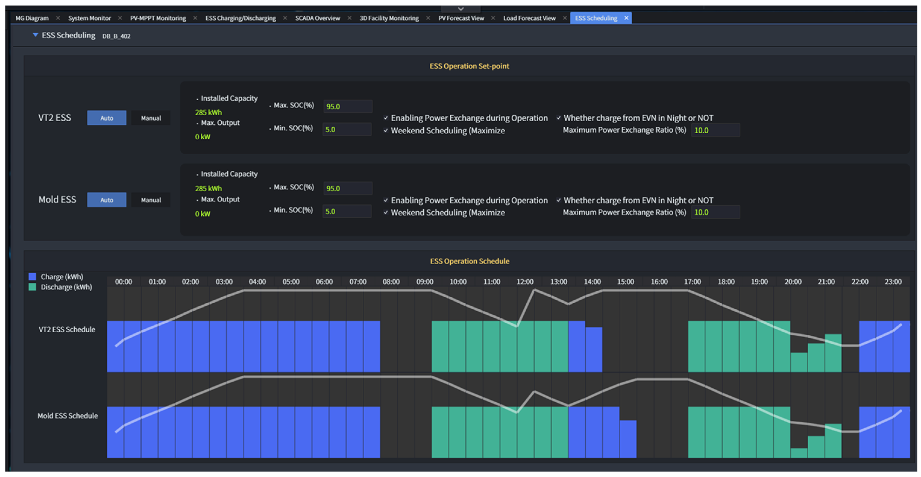
5.2.1. PSO Algorithm for ESS Scheduling

The PSO algorithm emulates the social behavior of particles in a swarm to find the global optimum. In this context, each particle represents a candidate ESS schedule vector that minimizes the total energy cost.

Objective: minimize total electricity cost over time:

$$\underset{P_{\mathit{ch}},P_{\mathit{dch}}}{\min }\sum _{t=1}^T\left(C_t·\left(P_{grid,t}+P_{dch,t}-P_{ch,t}\right)\right)$$

(6)

Subject to:

$${SOC}_{min}\le {SOC}_t\le {SOC}_{max}$$

$$0\le P_{ch,t},P_{dch,t}\le P_{max}$$

$${SOC}_{t+1}={SOC}_t+{\eta }_{ch}·P_{ch,t}·\Delta t-{\displaystyle \frac{1}{{\eta }_{dch}}}·P_{dch,t}·\Delta t$$

where

$C_t$: electricity price at time t;

$P_{ch,t},P_{dch,t}$: charging and discharging power;

${\eta }_{ch},{\eta }_{dch}$: charging/discharging efficiency;

${SOC}_t$: battery state of charge at time t.

To provide a clearer understanding of the PSO implementation, Figure 41 illustrates the detailed logic of the ESS scheduling algorithm and the swarm-based optimization process. In this study, the PSO algorithm utilizes a swarm size of 100, where each particle represents a candidate charge/discharge schedule for the ESS over a 24 h horizon. The particles are initialized randomly within feasible operational ranges, and their velocities and positions are updated iteratively based on inertia and acceleration parameters. The objective function is evaluated at each step, and the process converges within approximately 50 iterations. The global best solution obtained defines the optimal ESS schedule.

The DC-based multi-microgrid system allows energy sharing between VT2 and Mold. In the event of equipment failure or scheduling deviation, the system dynamically reallocates excess power where needed. The structure supports independent operation and cooperative balancing, improving the robustness of the overall EMS.

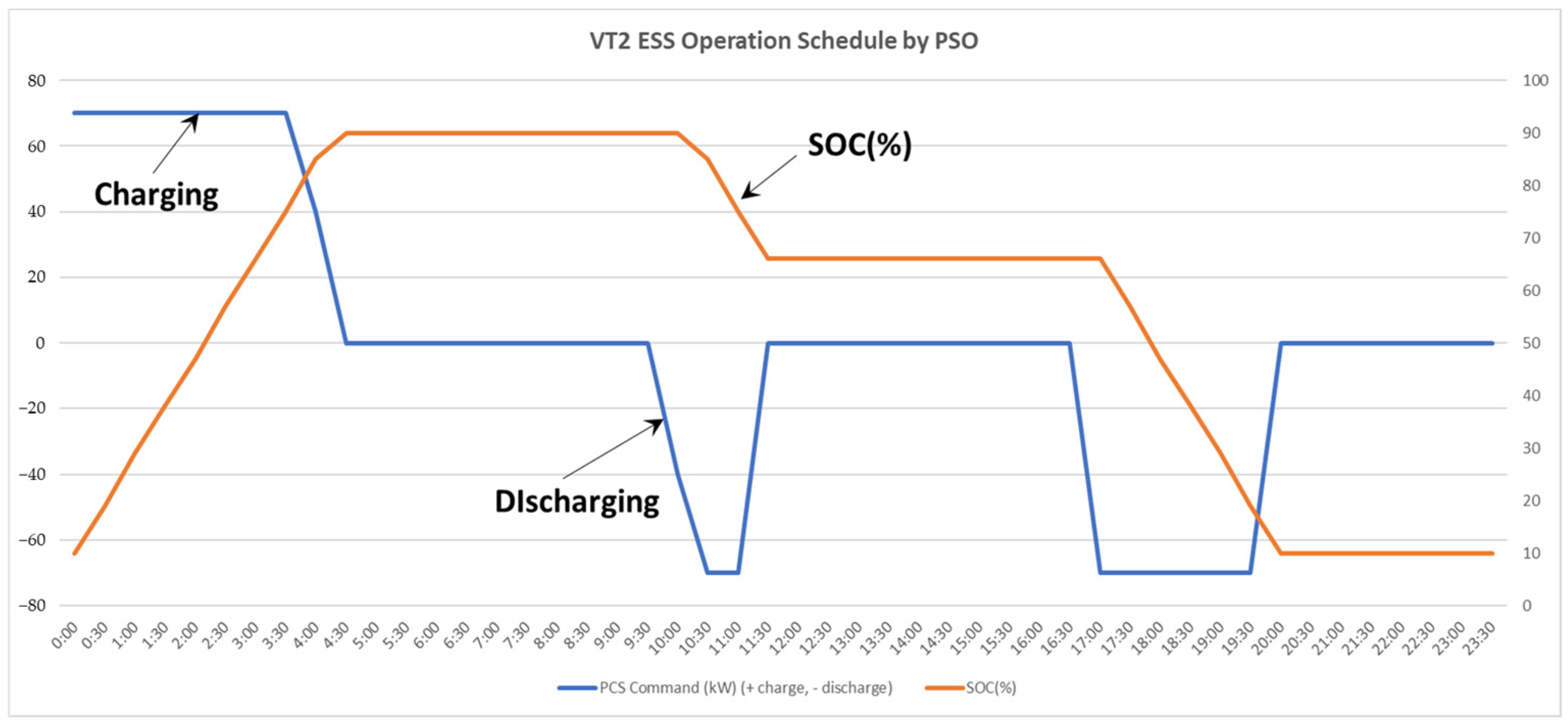
5.2.2. VT2 ESS Operation Results

Figure 42 presents the PSO-based operation schedule for the VT2 ESS with 30 min resolution. During the off-peak hours from midnight to early morning (00:00–05:00), the system performs aggressive charging to elevate the state of charge (SOC). Later, the battery discharges during peak pricing windows (09:00–11:00 and 17:00–19:00), corresponding to the predicted high-demand periods.

The SOC rises from 10 percent to 90 percent early in the day through continuous 70 kW charging, discharges at minus 70 kW during load peaks, and then stabilizes above 65 percent post-peak to maintain redundancy and supply backup.

This pattern demonstrates that the PSO-based control effectively anticipates future load using 24 h forecasts, prevents inefficient overlapping charge/discharge actions, and maintains battery longevity through shallow discharge cycles.

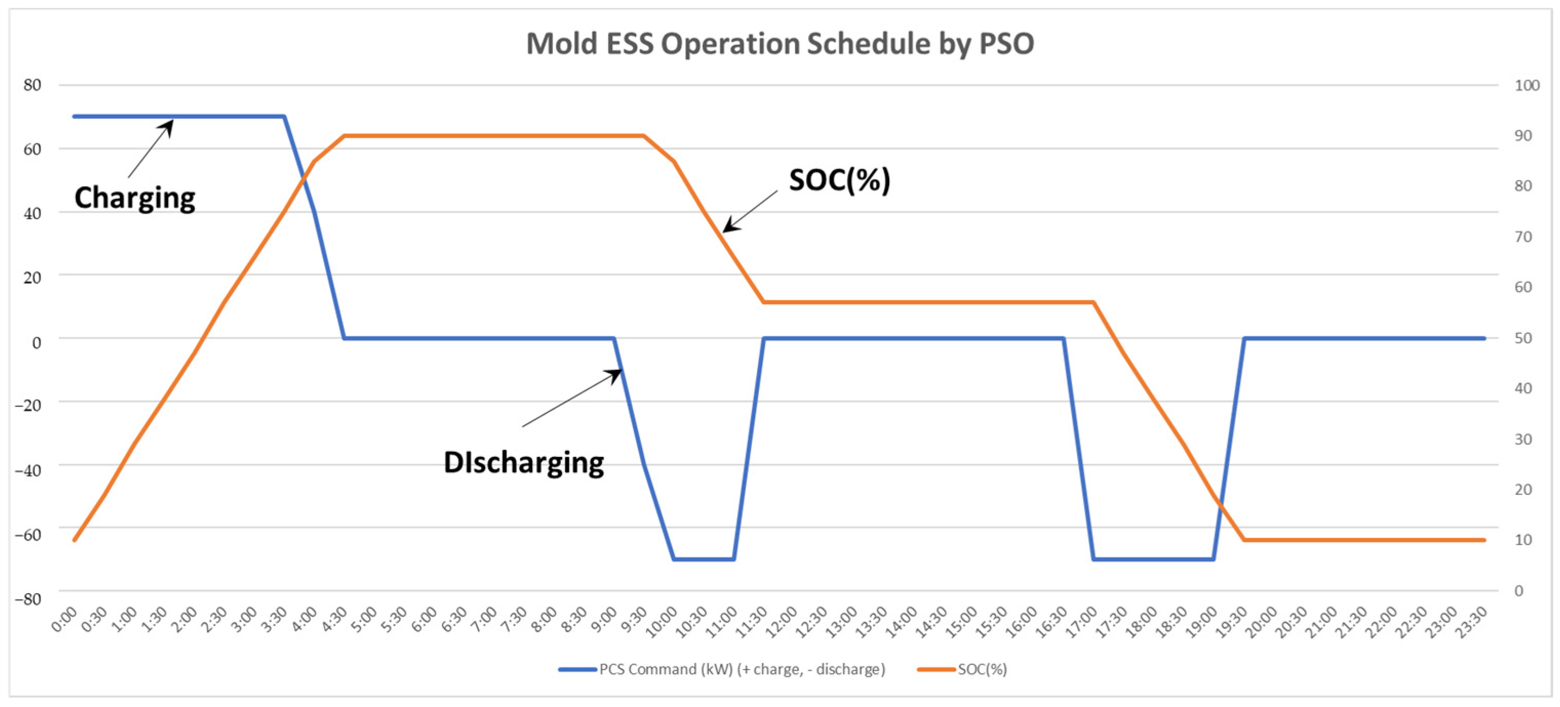
5.2.3. Mold ESS Operation Results

Figure 43 shows the PSO-generated schedule for the Mold ESS, which operates under the same control framework but with a more consistent load profile. The SOC increases steadily from 10 percent to 90 percent by 06:30 due to continuous overnight charging, then follows a two-stage discharge, first from 10:00 to 12:00 and again during the evening peak between 17:30 and 20:00.

Throughout the day, the SOC profile remains stable with minimal fluctuation, which is indicative of the steady-state operation of the Mold facility. This stable response enables Mold to engage in power trading activities efficiently while preserving its operational reliability.

While both VT2 and Mold ESS systems follow the same PSO-based scheduling approach, their operation patterns differ significantly: VT2 shows sharper SOC transitions due to more variable and peak-heavy load profiles, whereas Mold exhibits a smoother and more balanced charging–discharging behavior. This difference stems from the operational characteristics of each site—VT2’s production-based shifts lead to higher fluctuations, while Mold maintains a more constant load. As a result, Mold is better positioned to consistently participate in energy trading, while VT2 focuses on peak shaving and internal efficiency.

5.3. Multi-Microgrid Flexibility and Fault Resilience

In addition to energy forecasting and ESS scheduling, maintaining power quality under variable load and generation conditions is critical in industrial microgrid settings [21]. Figure 44 illustrates the real-time multi-microgrid (MG) operational structure deployed at the VT2 and Mold buildings, where distributed energy resources (DERs) such as photovoltaic (PV) systems and energy storage systems (ESS) are coordinated through an integrated Energy Management System (EMS).

Within the EMS, a Power Management System (PMS) supports key functions such as inverter parallel operation, fault-tolerant DER coordination, and real-time energy flow optimization based on load and generation forecasts, electricity tariffs, and ESS state of charge (SOC). It further contributes to system stability through features like inverter margin control, automatic restart, and AC voltage monitoring.

The PMS incorporates a PSO-based ESS scheduling algorithm, which considers building-specific load profiles, time-of-use pricing, and battery constraints to generate cost-optimized operational schedules. This approach enhances both economic performance and system flexibility.

As shown in Figure 45, the EMS autonomously generates charging and discharging schedules for each building. Both VT2 and Mold systems perform off-peak charging and peak-time discharging, but the patterns vary depending on site-specific load behavior. This demonstrates the EMS’s ability to implement adaptive, site-aware strategies using a shared optimization engine while preserving local autonomy and resilience.

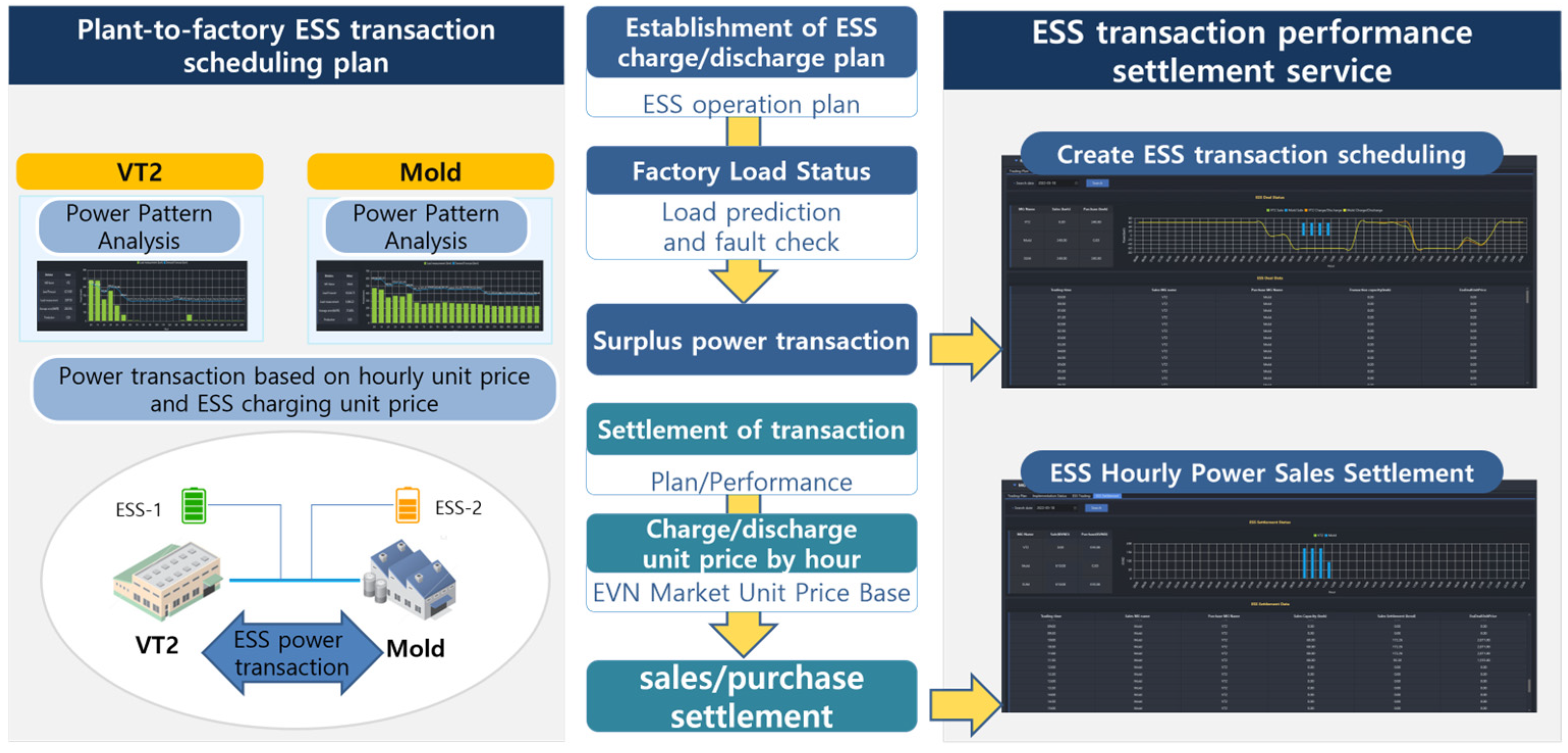
5.4. ESS Power Transaction and Settlement

The EMS facilitates power trading between VT2 and Mold based on predictive analytics. By using forecasted load demand, time-of-use electricity prices, and current SOC levels, the system generates a power trade plan that optimizes cost and balances surplus and deficit.

When VT2 accumulates excess energy during low-price charging periods, it supplies Mold during high-price intervals. This inter-facility transaction is automatically scheduled and managed within the EMS, as illustrated in Figure 46.

The platform also performs real-time execution and settlement of these trades. On 18 May, for example, Mold sold 240 kWh of power to VT2, generating a total revenue of 610.08 kVND. Detailed transaction records, including timestamps, exchanged energy, and corresponding settlement values, are continuously logged for audit and operational transparency, as illustrated in Figure 47 and Figure 48.

6. Conclusions

This study presented an integrated energy management strategy that combines load forecasting, economic operation scheduling, and inter-facility energy trading for industrial microgrids. By leveraging meteorological data and historical load information, an artificial neural network (ANN) model was developed to achieve a 24 h ahead forecast with an error margin within 12%. This predictive capability enabled the implementation of Particle Swarm Optimization (PSO)-based ESS scheduling tailored to site-specific consumption patterns.

The PSO algorithm successfully minimized operational costs by generating optimal charge/discharge schedules under time-of-use pricing and SOC constraints. Distinct operational behaviors were observed between VT2 and Mold sites due to differences in load variability, which the EMS accommodated effectively through dynamic schedule customization.

Furthermore, the deployment of a Power Management System (PMS) facilitated real-time control of DERs and multi-microgrid coordination. Through this system, surplus energy transactions between facilities were executed automatically, with corresponding financial settlements logged and verified.

While the current study focused on load forecasting, the integration of photovoltaic (PV) generation forecasting could further enhance the efficiency and economy of microgrid operations. Accurate supply-side forecasting would allow the EMS to better align generation and storage strategies, reduce curtailment, and improve renewable energy utilization.

In addition, future pricing models must evolve beyond simple time-of-use rates. Factors such as ESS state of health (SOH), the number of charge–discharge cycles, site-specific peak periods, and weekday-dependent tariff variations should be incorporated to enable truly optimized economic dispatch strategies.

Future research will expand on this by incorporating generation forecasts and developing coordinated scheduling algorithms for each component of the microgrid, including ESS, PV, and real-time pricing models. This modular optimization approach will further refine the system’s ability to deliver cost-effective and reliable energy management across diverse industrial environments.

These results demonstrate the feasibility and scalability of a forecast-driven EMS that enhances flexibility, reliability, and cost-efficiency in industrial microgrid environments. Future work may explore extensions to multi-site coordination involving external grids or market-driven dispatch frameworks. Additionally, from a system architecture perspective, future research should also address the development and deployment of a robust DC grid infrastructure. Such work is essential to support stable, bidirectional energy exchange and coordinated converter-based control strategies across interconnected microgrid units.

One limitation of this study is the absence of explicit photovoltaic (PV) power generation forecasting in the EMS framework. Although PV output profiles were considered in the simulation environment, real-time or day-ahead PV prediction was not integrated into the control strategy. Incorporating accurate PV forecasting—using machine learning or hybrid models—would significantly enhance the effectiveness of PSO-based scheduling and enable more proactive coordination between renewable generation and energy storage systems.

In addition, the current EMS utilizes a simplified time-of-use (TOU) pricing model, which does not fully reflect practical economic dispatch conditions. Future research will incorporate advanced pricing mechanisms that account for the state of health (SOH) of ESS, degradation from charge/discharge cycles, dynamic price fluctuations, and site-specific peak periods. These enhancements will allow for more realistic and cost-optimized energy management, enabling the EMS to operate effectively in more complex and variable industrial microgrid environments. Future work will thus aim to jointly optimize both load and PV forecasts while integrating dynamic, cost-aware dispatch models to establish a more robust, adaptive, and economically efficient EMS.

References

1. Heldeweg, M.A.; Séverine, S. Renewable energy communities as ‘socio-legal institutions’: A normative frame for energy decentralization? Renew. Sustain. Energy Rev. 2020, 119, 109518. [Google Scholar] [CrossRef]
2. Urishev, B. Decentralized Energy Systems, Based on Renewable Energy Sources. Appl. Sol. Energy 2019, 55, 207–212. [Google Scholar] [CrossRef]
3. Yaqoot, M.; Diwan, P.; Kandpal, T.C. Review of barriers to the dissemination of decentralized renewable energy systems. Renew. Sustain. Energy Rev. 2016, 58, 477–490. [Google Scholar] [CrossRef]
4. Kim, J.S.; So, S.M.; Kim, J.-T.; Cho, J.-W.; Park, H.-J.; Jufri, F.H.; Jung, J. Microgrids platform: A design and implementation ofcommon platform for seamless microgrids operation. Electr. Power Syst. Res. 2019, 167, 21–38. [Google Scholar] [CrossRef]
5. Zheng, X.; Yang, M.; Yu, Y.; Wang, C. Short-Term Net Load Forecasting for Regions with Distributed Photovoltaic Systems Based on Feature Reconstruction. Appl. Sci. 2023, 13, 9064. [Google Scholar] [CrossRef]
6. Kong, W.; Dong, Z.Y.; Jia, Y.; Hill, D.J.; Zhang, Y. A Review of Deep Learning Methods for Short-Term Load Forecasting. In Proceedings of the 2021 International Conference on Smart Grid and Electrical Automation (ICSGEA 2021), Kunming, China, 29–30 May 2021; Springer: Singapore, 2021; pp. 485–494. [Google Scholar] [CrossRef]
7. Wang, J.; Liu, H.; Zheng, G.; Li, Y.; Yin, S. Short-Term Load Forecasting Based on Outlier Correction, Decomposition, and Ensemble Reinforcement Learning. Energies 2023, 16, 4401. [Google Scholar] [CrossRef]
8. Hamidi, M.; Raihani, A.; Bouattane, O. Sustainable Intelligent Energy Management System for Microgrid Using Multi-Agent Systems: A Case Study. Sustainability 2023, 15, 12546. [Google Scholar] [CrossRef]
9. Gutiérrez-Oliva, D.; Colmenar-Santos, A.; Rosales-Asensio, E. A Review of the State of the Art of Industrial Microgrids Based on Renewable Energy. Electronics 2022, 11, 1002. [Google Scholar] [CrossRef]
10. Ginzburg-Ganz, E.; Segev, I.; Balabanov, A.; Segev, E.; Kaully Naveh, S.; Machlev, R.; Belikov, J.; Katzir, L.; Keren, S.; Levron, Y. Reinforcement Learning Model-Based and Model-Free Paradigms for Optimal Control Problems in Power Systems: Comprehensive Review and Future Directions. Energies 2024, 17, 5307. [Google Scholar] [CrossRef]
11. Lv, L.; Wu, Z.; Zhang, L.; Gupta, B.B.; Tian, Z. An Edge-AI Based Forecasting Approach for Improving Smart Microgrid Efficiency. IEEE Trans. Ind. Inform 2022, 18, 7946–7954. [Google Scholar] [CrossRef]
12. Taylor, J.W.; McSharry, P.E.; de Menezes, L.M. A Comparison of Univariate Methods for Forecasting Electricity Demand up to a Day Ahead. Int. J. Forecast. 2006, 22, 1–16. [Google Scholar] [CrossRef]
13. Yildiz, H.B. Modeling and Forecasting Electricity Consumption of Residential Consumers by Using the ARIMA and Hybrid Models. Energy 2017, 124, 117–127. [Google Scholar] [CrossRef]
14. Zhang, Y.; Wang, X.; Li, Y.; Liu, Y. Load Forecasting with Machine Learning and Deep Learning Methods. Appl. Sci. 2022, 13, 7933. [Google Scholar] [CrossRef]
15. Li, X.; Peng, J.; Zhang, Y.; Lu, S. Short-Term Load Forecasting for Microgrids Based on LSTM Recurrent Neural Network. Sustain. Cities Soc. 2023, 104775. [Google Scholar] [CrossRef]
16. Li, Q.; Sun, H.; Zhang, L.; Wen, Y.; Ma, C. Short-Term Load Forecasting Using a Deep Neural Network. Energies 2020, 13, 3870. [Google Scholar] [CrossRef]
17. Toure, I.; Payman, A.; Camara, M.-B.; Dakyo, B. Energy Management in a Renewable-Based Microgrid Using a Model Predictive Control Method for Electrical Energy Storage Devices. Electronics 2024, 13, 4651. [Google Scholar] [CrossRef]
18. Shi, L.; Cen, Z.; Li, Y.; Wu, F.; Lin, K.; Yang, D. Distributed Optimization of Multi-Microgrid Integrated Energy System with Coordinated Control of Energy Storage and Carbon Emissions. Sustainability 2024, 16, 3225. [Google Scholar] [CrossRef]
19. Merabet, A.; Al-Durra, A.; El Fouly, T.; El-Saadany, E.F. Multifunctional energy management system for optimized network of microgrids considering battery degradation and load adjustment. J. Energy Storage 2024, 100, 113709. [Google Scholar] [CrossRef]
20. Deb, C.; Zhang, F.; Yang, J.; Lee, S.E.; Shah, K.K. A Review on Time Series Forecasting Techniques for Building Energy Consumption. Renew. Sustain. Energy Rev. 2017, 74, 902–924. [Google Scholar] [CrossRef]
21. Ko, J.-h. High-Definition Dynamic Voltage Restorer Systems Using Equivalent Time Sampling Techniques and Circular Structural Memory Filters. Appl. Sci. 2024, 14, 6896. [Google Scholar] [CrossRef]
Figure 1. Overview of microgrid construction in Ho Chi Minh Industrial Complex.
Energies 18 03202 g001
Figure 2. Configuration diagram of multiple microsystems based on DC grid.
Energies 18 03202 g002
Figure 3. Example of Ho Chi Minh meteorological data.
Energies 18 03202 g003
Figure 4. Temperature data.
Energies 18 03202 g004
Figure 5. Dew point data.
Energies 18 03202 g005
Figure 6. Humidity data.
Energies 18 03202 g006
Figure 7. Wind speed data.
Energies 18 03202 g007
Figure 8. VT2 load pattern.
Energies 18 03202 g008
Figure 9. Mold load pattern.
Energies 18 03202 g009
Figure 10. Kindergarten load pattern.
Energies 18 03202 g010
Figure 11. VT2 load vs. temperature.
Energies 18 03202 g011
Figure 12. VT2 load vs. dew point.
Energies 18 03202 g012
Figure 13. VT2 load vs. humidity.
Energies 18 03202 g013
Figure 14. VT2 load vs. wind speed.
Energies 18 03202 g014
Figure 15. Mold load vs. temperature.
Energies 18 03202 g015
Figure 16. Mold load vs. dew point.
Energies 18 03202 g016
Figure 17. Mold load vs. humidity.
Energies 18 03202 g017
Figure 18. Mold load vs. wind speed.
Energies 18 03202 g018
Figure 19. Kindergarten load vs. temperature.
Energies 18 03202 g019
Figure 20. Kindergarten load vs. dew point.
Energies 18 03202 g020
Figure 21. Kindergarten load vs. humidity.
Energies 18 03202 g021
Figure 22. Kindergarten load vs. wind speed.
Energies 18 03202 g022
Figure 23. Histogram of daily Pearson correlation coefficients between VT2 load and temperature.
Energies 18 03202 g023
Figure 24. Histogram of daily Pearson correlation coefficients between VT2 load and dew point.
Energies 18 03202 g024
Figure 25. Histogram of daily Pearson correlation coefficients between VT2 load and humidity.
Energies 18 03202 g025
Figure 26. Histogram of daily Pearson correlation coefficients between VT2 load and wind speed.
Energies 18 03202 g026
Figure 27. Histogram of daily Pearson correlation coefficients between Mold load and temperature.
Energies 18 03202 g027
Figure 28. Histogram of daily Pearson correlation coefficients between Mold load and dew point.
Energies 18 03202 g028
Figure 29. Histogram of daily Pearson correlation coefficients between Mold load and humidity.
Energies 18 03202 g029
Figure 30. Histogram of daily Pearson correlation coefficients between Mold load and wind speed.
Energies 18 03202 g030
Figure 31. Histogram of daily Pearson correlation coefficients between kindergarten load and temperature.
Energies 18 03202 g031
Figure 32. Histogram of daily Pearson correlation coefficients between kindergarten load and dew point.
Energies 18 03202 g032
Figure 33. Histogram of daily Pearson correlation coefficients between kindergarten load and humidity.
Energies 18 03202 g033
Figure 34. Histogram of daily Pearson correlation coefficients between kindergarten load and wind speed.
Energies 18 03202 g034
Figure 35. Overall structure and algorithmic flow of the ANN-based forecasting model, including input data sources, neural network architecture, and K-fold cross-validation for hyperparameter optimization.
Energies 18 03202 g035
Figure 36. Actual vs. predicted load—VT2.
Energies 18 03202 g036
Figure 37. Actual vs. predicted load—Mold.
Energies 18 03202 g037
Figure 38. Actual vs. predicted load—Kindergarten.
Energies 18 03202 g038
Figure 39. Overview of the load forecasting system using local weather, historical load data, and ANN model.
Energies 18 03202 g039
Figure 40. Comparison of actual measured load and ANN-based forecast results for VT2 and Mold on 17 May 2022.
Energies 18 03202 g040
Figure 41. ESS scheduling algorithm and PSO optimization logic illustrating particle initialization, evaluation, and convergence.
Energies 18 03202 g041
Figure 42. PSO-based ESS command and SOC profile for VT2 on a 30 min interval.
Energies 18 03202 g042
Figure 43. PSO-based ESS command and SOC profile for Mold on a 30 min interval.
Energies 18 03202 g043
Figure 44. DER-integrated multi-microgrid control system with PMS and PSO-based scheduling algorithm.
Energies 18 03202 g044
Figure 45. Automatically generated ESS operation schedule and SOC profile for VT2 and Mold.
Energies 18 03202 g045
Figure 46. Overall ESS transaction scheduling system and workflow from forecasting to settlement.
Energies 18 03202 g046
Figure 47. ESS transaction scheduling between VT2 and Mold based on forecasted surplus power and time-of-use pricing.
Energies 18 03202 g047
Figure 48. ESS deal status and financial settlement records for VT2 and Mold on 18 May.
Energies 18 03202 g048