Correlational Analysis of Relationships Among Nodal Powers and Currents in a Power System

Abstract

This paper concerns the analysis of the impact of nodal powers on currents flowing in the power system (PS). Two problems are considered here, i.e., Problem I—identifying the branches of the PS on which currents have magnitudes that strongly change with changes in nodal powers, characterized by magnitudes and arguments, and identifying nodes at which these powers exist, and Problem C—PS clustering from the point of view of the relationships between branch current magnitudes (BCMs) and nodal power magnitudes (nodal apparent powers—NAPs) or nodal power arguments (NPAs). The solution to Problem I may be useful for the modernization of the PS as well as in the practice of dispatchers. The solution to Problem C may be useful in system analyses. The analysis of the literature shows that the existing papers only touch on the earlier-formulated problems to a modest extent. In fact, those problems are not solved. The paper fills this gap by presenting methods for solving the given problems. Both considered problems are solved using data mining. The investigation of correlational relationships (CRs) between BCMs and NAPs as well as CRs between BCMs and NPAs is used. Any such strong CR indicates large changes in BCM with changes in NAP or NPA remaining in the considered CR. Nodes, which through NAPs are in CRs with BCM for a selected branch, are a cluster associated with this branch. The paper also considers clusters encompassing branches, for each of which BCMs are in CRs with the NAP of a given node. Similarly, when searching for clusters encompassing nodes, or clusters encompassing branches, in the aforementioned CRs, one considers NPAs instead of NAPs. The paper proposes methods for solving Problem I and Problem C, which allow (i) relatively simple detection of regularities in the PS with the provision of their statistical evaluation, which would be difficult or impossible in the case of other methods, and (ii) solving the indicated problems based only on measurement data, and do not require (i) performing flow calculations and (ii) large computational effort. The paper presents the properties of the methods on the examples of the IEEE 14-Bus Test System and IEEE 30-Bus Test System.

1. Introduction

Power flow analysis in a power system (PS) can be used for various purposes, in particular to determine (i) how close to constraints the currents (current magnitudes) are in individual branches, (ii) how large the active power losses are in the branches, (iii) how large the voltage drops are in the branches and, consequently, how much the voltages (their magnitudes) will decrease at the nodes of the PS. In each of the above cases, the larger the currents on the branches are, the less favorable the situation is. Therefore, special attention should be paid to those branches on which the currents increase the most. Currents in PS are a function of the loads and, consequently, of the generation in this system, i.e., a function of the nodal powers. The presented statements indicate the validity of the formulation of the following questions: Question 1—“On which branches are the flow currents whose magnitudes change strongly with the change in nodal powers?” Question 2—“At which nodes are there nodal powers that significantly influence the changes in the current magnitudes on a given branch?”

The answers to the following questions are also interesting: Question 3—“At which nodes of the PS do changes in nodal powers have a strong influence on changes in branch currents?” Question 4—“Which branches show changes in branch currents, as mentioned in Question 3, that are clearly related to changes in the nodal power at each node individually?”

Question 1 and Question 3 define the identification problem (Problem I), and Question 2 and Question 4 define the PS clustering problem (Problem C).

Problem I and Problem C are related to the analysis of the impact of nodal powers on the power flow in the PS. Similar analyses were considered in existing papers. In [1], using the perturbation theory [2], the impact of changes in nodal powers (active or reactive) on changes in branch powers (active or reactive) was considered.

In [1], only some nodal powers were taken into account. These are nodal powers associated with the sources of renewable energy. In [3], it was assumed that (i) the considered nodal powers are unknown but bounded, (ii) the PS model is linearized, and (iii) the uncertainties characterizing the considered nodal powers are propagated through the linearized model. The results of the calculations were the worst-case deviations of magnitudes and arguments of nodal voltages.

In [4], the authors presented the sensitivity matrix of the changes in the magnitudes of nodal voltages relative to the changes in the reactive nodal powers in the PS.

Previously, only some papers were cited, which presented different possible approaches to solving the problem of analyzing the impact of nodal powers on the power flow in a PS, considered directly or indirectly through the impact of nodal powers on nodal voltages.

To summarize, a review of existing papers showed that the methods proposed therein involved complex calculations and were not very accurate. Generally, these methods referred to a snapshot of the PS state. However, the situation in the PS may be different for other snapshots.

The analyses leading to the answers to Question 2 and Question 4 are supplementary to the analyses leading to the answers to Question 1 and Question 3. The answer to Question 1 allows us to identify the branches of the PS where there are currents that change strongly with changes in nodal powers without indicating the nodes at which these powers occur. In turn, the answer to Question 3 allows us to identify the nodes of the PS where there are nodal powers that strongly affect the branch currents without indicating the branches on which these currents occur. For each branch, the answer to Question 2 defines the area of the PS by specifying the nodes at which there are nodal powers that significantly affect the current on the considered branch. The answer to Question 4 defines the area of the PS by specifying the branches on which the currents are significantly affected by the nodal power of the considered node.

It is easy to see that the answers to Question 2 and Question 4 define clusters in the PS [5]. There are many papers describing different clustering methods in general, e.g., [5,6,7,8], and in relation to PS, e.g., [9,10,11,12,13]. In papers on the PS, methods for similarity-based clustering are presented [9,10,11,12,13]. Objects that are considered in clustering are characterized by attributes. The similarity of the objects is determined based on these attributes. The following categories of similarity measures can be given [5]:

• Difference-based measures—a family of parameterized distances, called the Minkowski distance, Canberra distance, Hamming distance, and Gower’s coefficient.
• Correlation-based measures—the cosine measure, Pearson’s correlation measure, and Spearman’s correlation measure.

There are no strict requirements for clustering methods [5]. Substantially different approaches to clustering are used. Clustering methods, being frequently used, are as follows:

• k-Centers clustering (k-means, k-medians, k-medoids, and adaptive k-centers),
• Hierarchical clustering,
• Support vector machines,
• Support vector regression,
• Kohonen’s self-organizing maps (SOM).

Ref. [9] considers clustering of load patterns. Various clustering techniques are taken into consideration. The properties of those techniques are discussed. Clustering as a data mining technique is used to extract underlying patterns from energy consumptions.

Ref. [10] deals with aggregation of time-series input data to representative periods. In this case, the clustering technique can be used. This can be seen in the example of optimizing battery charging/discharging and gas turbine operation scheduling. Conventionally used methods and shape-based clustering methods are compared.

In [11], optimal PS clustering is used for the aim of controlled islanding. One proposes a decomposition of the adjacency matrix of a network using a spectral clustering algorithm.

Refs. [12,13] assume a correlation approach to PS clustering. In [12], correlations between nodal reactive powers and branch reactive powers are studied. For clustering purposes, Ref. [13] takes into account the correlation of (i) nodal apparent powers and branch apparent powers and (ii) arguments of nodal powers and branch apparent powers. In [12], as well as in [13], hard clustering is presented.

In the existing papers, there are no answers to Question 2 and Question 4, which were defined earlier. Each of these questions points to appropriately defined clusters. The objects that are elements of those clusters are nodes and branches of the PS in the case of Question 2 and Question 4, respectively. In the case of Question 2, the attribute of the node is the fact of the significance of the relationship between the nodal power at this node and the current on a precisely defined branch. In the case of Question 4, the attribute of the branch is the fact of the significance of the relationship between the current on this branch and the nodal power at a precisely defined node. Objects that are taken into account when searching for an answer to Question 2 as well as Question 4 are similar, if each of them individually has the same attribute referring to the significance of the relationship considered in its case. There are no solutions to such defined tasks in the literature.

The literature shows that there are papers that provide solutions to problems that are more or less similar to the problems addressed in this paper. However, there is no paper that solves the problems indicated by the questions formulated at the beginning of the section. Consequently, the aim of this paper is to present original, computationally advantageous methods that allow for the analysis of the influence of nodal powers on the currents flowing in the PS.

That aim is achieved through:

• Developing an approach to planned analyses.
• Using the adopted approach, developing original methods allowing for solving Problem I and Problem C.
• Presentation of the use of the developed methods in a case study, in which the IEEE 14-Bus Test System [14] (TS14) and IEEE 30-Bus Test System (TS30) [15] are considered.
• Presentation of the properties of the proposed method.

Further considerations are given in the following sections. In Section 2, the approach taken to solving the problems defined earlier is presented. Section 3 justifies the adoption of the Kendall’s rank correlation coefficient (KRCC) as a measure of the strength of correlation between the considered quantities. This correlation coefficient is used in the methods described in Section 4. Section 5 shows the application of the proposed methods to the analysis of the IEEE 14-Bus Test System and IEEE 30-Bus Test System, when the entire set of system operating states, for which data on the considered quantities are possessed, is taken into account. Section 6 deals with the analyses assuming that the system operating states are subsets of the aforementioned set of states. The discussion of the computational results given in Section 5 and Section 6 is given in Section 7. The conclusions of the considerations carried out in the paper are given in Section 8.

2. Correlational Approach to Solving the Considered Problems

At any time, the energy delivered to the PS should cover the consumers’ demand for electrical energy and the losses of this energy during its transmission from the place of generation to the place of its utilization. The individual loads and, as a result, the generation powers change over time. These changes cannot be determined deterministically. With changes in loads and generation powers (collectively called nodal powers), active and reactive power flows in the PS and, consequently, currents on the PS branches change. In this situation, stochastic description can be used to describe phenomena in the PS. To solve the problems, which are considered in the paper, relationships between branch current magnitudes (BCMs) and the nodal apparent powers (NAPs), as well as relationships between BCMs and the nodal power arguments (NPAs), should be taken into account. For the purposes of the described approach, correlational relationships (CRs) between the distinguished quantities can be used. CRs simply say that two considered variables perform in a synchronized manner [16].

The correlation approach to solving problems in the PS is used in other papers (e.g., [12,13,14,15,17,18,19,20,21,22,23]). However, no other paper has used this approach to solve the problems discussed in this paper.

The investigations of CRs allows us to determine the strength of the relationships between BCMs and NAPs, as well as the strength of the relationships between BCMs and NPAs. Those investigations make it possible to identify the branches of the PS on which currents are strongly related to nodal powers. Such a strong relationship means that when the NAP or NPA changes, there is a significant change in the considered BCM. In particular, an increase in the NAP or NPA may result in an increase in the BCM. The previously mentioned relationship may also mean a decrease in the BCM with an increase in the NAP or NPA. Stochastic investigation means that it is not enough to examine only the strength of CRs, but also the statistical significance of these relationships must be established. For the purposes of examining the relationships between BCMs and NAPs or between BCMs and NPAs, only statistically significant correlational relationships (SSCRs) should be taken into account.

3. Investigation of Correlational Relationships Between Distinguished Quantities

When examining CRs, it is important to determine the strength of association of the considered quantities. Various correlation coefficients were used as measures of this strength. The most well-known correlation coefficients are (i) the Pearson product–moment correlation coefficient (Pearson’s correlation coefficient), (ii) the Spearman’s rank correlation coefficient (Spearman’s rho), and (iii) the Kendall’s rank correlation coefficient (KRCC) [24,25]. Following the order adopted in the previous sentence, the mentioned correlation coefficients are used for relationships that are (i) linear, (ii) monotonic, and (iii) non-linear and non-monotonic, respectively.

Further considerations were carried out to determine which of the correlation coefficients is the most appropriate when looking for a solution to Problem I and Problem C.

The current on a branch of the PS can be determined as a result of measurement using a PMU device, or it can be calculated on the basis of measurements of active and reactive power flows on the branch. The PMU device allows for obtaining the current phasor, i.e., its magnitude and argument. For the purposes of the considerations given in this paper, it is necessary to know the BCMs. If there is no measurement of the current phasor, but only measurements of active and reactive power flows, then the magnitude of the branch current on branch b_{i_j} (represented by the Π model shown in Figure 1), i.e., a branch between nodes n_i and n_j, where n_i is a node in the PS with number i, can be calculated from the formula:

$$I_{ij}={\displaystyle \frac{\sqrt{P_{ij}^2+Q_{ij}^2}}{V_i}},$$

(1)

where I_ij is the magnitude of the current on branch b_{i_j} at node n_i, P_ij and Q_ij are active and reactive power flows on branch b_{i_j} at node n_i, respectively, and V_i is the magnitude of the voltage at node n_i.

Power flows P_ij and Q_ij are related to the nodal voltages V_i and V_j:

$$P_{ij}=\mathrm{R}\mathrm{e} {\mathbf{S}}_{ij}, Q_{ij}=\mathrm{I}\mathrm{m} {\mathbf{S}}_{ij},$$

(2)

where ${\mathbf{S}}_{ij}$ is a complex power flow on branch b_{i_j} at end i:

$${\mathbf{S}}_{ij}={\mathbf{V}}_i{\mathbf{I}}_{ij}^{\ast }={\mathbf{V}}_i{\mathbf{V}}_j^{\ast }/{\mathbf{z}}_{ij}^{\ast }-V_i^2\left(1/{\mathbf{z}}_{ij}^{\ast }+{\mathrm{y}}_{ij}^{\ast }\right).$$

(3)

Power flows P_ji and Q_ji are given by the formulas:

$$P_{ji}=\mathrm{R}\mathrm{e} {\mathbf{S}}_{ji},Q_{ji}=\mathrm{I}\mathrm{m} {\mathbf{S}}_{ji},$$

(4)

where ${\mathbf{S}}_{ji}$ is a complex power flow on branch b_{j_i} at end j:

$${\mathbf{S}}_{ji}={\mathbf{V}}_j{\mathbf{I}}_{ji}^{\ast }={\mathbf{V}}_j{\mathbf{V}}_i^{\ast }/{\mathbf{z}}_{ij}^{\ast }-V_j^2\left(1/{\mathbf{z}}_{ij}^{\ast }+{\mathit{y}}_{ji}^{\ast }\right).$$

(5)

Based on (2) and (4), it can be concluded that, in general:

$$P_{ij}\ne P_{ji},Q_{ij}\ne Q_{ji}.$$

(6)

Also, if any of the active or reactive power flows are different from zero, then (see Appendix A in [17]):

$$V_i\ne V_j.$$

(7)

In consequence,

$$I_{ij}\ne I_{ji}.$$

(8)

Nodal voltages in the PS depend on the nodal active and reactive powers, or, in other words, on the nodal complex powers.

A conjugate complex power for node n_k k ∈ {1, 2, …, n}, where n is the number of nodes in the PS, is as follows:

$${\mathbf{S}}_k^{\ast }=P_k-\mathrm{j}{Q}_k={\mathbf{V}}_k^{\ast }{\sum }_{l=1}^{\mathrm{n}}{\mathbf{Y}}_{kl}{\mathbf{V}}_{\mathit{l}},$$

(9)

where P_k and Q_k are nodal active and reactive powers, respectively, and Y_kl is an element of the admittance matrix.

The magnitude and argument of the k-th complex nodal power can be calculated from the formulas:

$$S_k=\sqrt{P_k^2+Q_k^2},$$

(10)

$${\phi }_k=\mathrm{a}\mathrm{r}\mathrm{c}\mathrm{t}\mathrm{a}\mathrm{n}\left(Q_k/P_k\right).$$

(11)

The presented considerations indicate that the relationship between BCM I_ij and NAP S_k, as well as between BCM I_ij and NPA φ_k, is non-linear. According to [23,24], the appropriate measure for assessing CRs between BCMs and NAPs or CRs between BCMs and NPAs is the KRCC. The formula for the KRCC is as follows:

$$t_{\mathrm{k},\mathrm{U}-\mathrm{W}}=\left(c-d\right)/\left(c+d\right) ,$$

(12)

where t_k,U-W stands for KRCC, characterizing CR between quantities U and W, while c and d are the numbers of concordant and discordant pairs of observations (U_i, W_i) i ∈ {1, 2, …, m} in the sample, respectively.

If U_j < U_k and W_j < W_k or U_j > U_k and W_j > W_k, then (U_j, W_j) and (U_k, W_k) are concordant, and in other cases, (U_j, W_j) and (U_k, W_k) are discordant.

For the aim of interpreting the size of the KRCC, which characterizes each of the considered CRs, the rule of thumb is shown in

Table 1. Rule of thumb of interpreting the size of the KRCC [26].

Strenght of Association	KRCC
	Positive	Negative
Very small	<0.1	>−0.1
Small	[0.1, 0.3)	(−0.3, −0.1]
Medium	[0.3, 0.5)	(−0.5, −0.3]
Large	[0.5, 1.0]	[−1.0, −0.5]

.

Hereafter, cr_U-W stands for the CR between U and W.

4. Proposed Methods

4.1. Method I—Method of Finding Branches with Currents Statistically Significantly Correlated with Nodal Powers and Indicating the Nodes at Which These Powers Are

Method I is the method proposed to solve Problem I. Method I consists of the following steps:

• Step 0

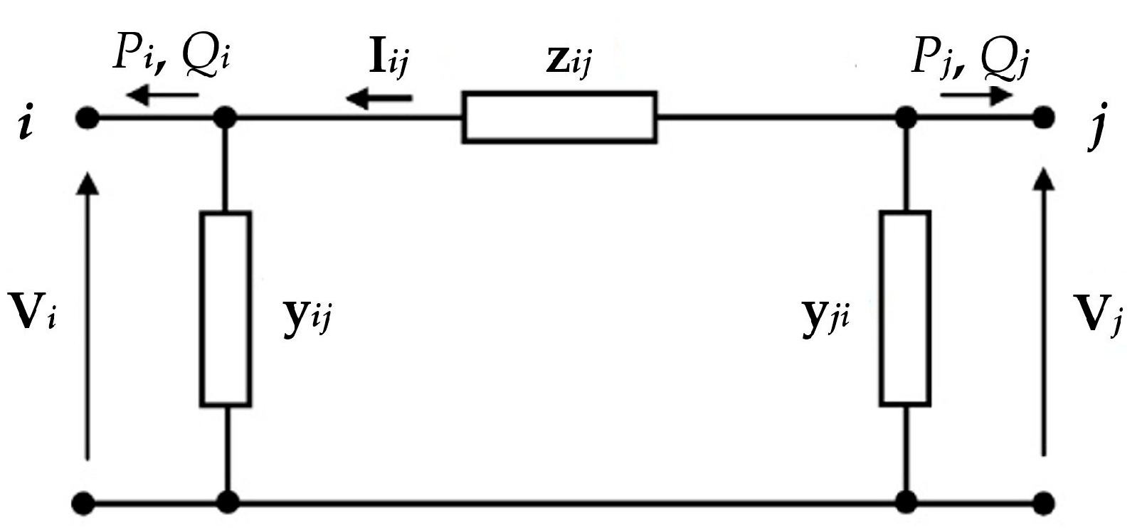
• Creation of datasets of magnitudes of individual currents at the ends of the PS branches:
  • if current phasors are measured at the ends of the branches of the PS, then elements of the sets of observations of BCMs are measurements of the BCMs,
  • if active and reactive power flows are measured at the ends of the branches of the PS, then elements of the set of observations of BCMs are results of calculations using Formula (1).
• Creation of datasets of NAPs and NPAs, calculated on the basis of active and reactive nodal powers in accordance with Formulas (10) and (11), respectively.

• Step 1

• Analyses of CRs between BCMs and NAPs:
  • Calculation of KRCCs for CRs between magnitudes of the currents at the ends of the PS branches and NAPs.
    For each branch, among the two CRs between the magnitudes of currents at the branch ends and NAP S_k k ∈ {1, 2, …, n}, select the CR for which the absolute value of the KRCC is larger. The selected CR is the characteristic CR between the magnitude of the current on the considered branch and NAP S_k k ∈ {1, 2, …, n}.
  • Creation of set $S_{\mathrm{I}-\mathrm{S}}$, the elements of which are characteristic CRs between BCMs and NAPs.
• Analyses of CRs between BCMs and NPAs:
  • Calculation of KRCCs for CRs between magnitudes of the currents at the ends of the PS branches and NPAs.
    For each branch, among the two CRs between the magnitudes of currents at the branch ends and NPA φ_k k ∈ {1, 2, …, n}, select the CR for which the absolute value of the KRCC is larger. The selected CR is the characteristic CR between the magnitude of the current on the considered branch and NPA φ_k k ∈ {1, 2, …, n}.
  • Creation of set $S_{\mathrm{I}-\phi }$, the elements of which are characteristic CRs between BCMs and NPAs.

• Step 2

• Performing significance tests of all CRs from set $S_{\mathrm{I}-\mathrm{S}}$.

In each of such significance tests, the following statistic is used [25]:

$$z={\displaystyle \frac{3t_{\mathrm{k},\mathrm{U}-\mathrm{W}}\sqrt{\mathrm{m}\left(\mathrm{m}-1\right)}}{\sqrt{2\left(2\mathrm{m}+5\right)}}}.$$

(13)

The statistic z is approximately distributed as a standard normal under the assumption that the considered variables are statistically independent.

2.

Creating set $S_{\mathrm{S},\mathrm{I}-\mathrm{S}}$, the elements of which are SSCRs between BCMs and NAPs, and these CRs are elements of set $S_{\mathrm{I}-\mathrm{S}}$.

3.

Performing significance tests of all CRs from set $S_{\mathrm{I}-\phi }$, using the statistic (13).

4.

Creating set $S_{\mathrm{S},\mathrm{I}-\phi }$, the elements of which are SSCRs between BCMs and NPAs, and these CRs are elements of set $S_{\mathrm{I}-\phi }$.

• Step 3

• Creating sets $S_{\mathrm{S},\mathrm{I}-\mathrm{S}}^{range}$ and $S_{\mathrm{S},\mathrm{I}-\phi }^{range}$, being subsets of sets $S_{\mathrm{S},\mathrm{I}-\mathrm{S}}$ and $S_{\mathrm{S},\mathrm{I}-\phi }$, respectively. For each element of set $S_{\mathrm{S},\mathrm{I}-\mathrm{S}}^{range}$ as well as set $S_{\mathrm{S},\mathrm{I}-\phi }^{range}$, the absolute value of the KRCC is in the interval range.

• Step 4

• Creating ordered set $A_{\mathrm{B}}^{\mathrm{r}\mathrm{a}\mathrm{n}\mathrm{g}\mathrm{e}}$ containing branches, each of which is characterized by the fact that the current flowing on it has a magnitude that is in SSCRs belonging to set $S_{\mathrm{S},\mathrm{I}\_\mathrm{S}}^{range}$ or set $S_{\mathrm{S},\mathrm{I}\_\phi }^{range}$.
  The branches in set $A_{\mathrm{B}}^{range}$ are arranged in decreasing order of the absolute values of the KRCCs for the CRs between BCMs and NAPs or for the CRs between BCMs and NPAs. The branch that is in the first position is the one on which there is a current with the magnitude remaining in the strongest CR with a specific NAP or a specific NPA. One branch appears only once in set $A_{\mathrm{B}}^{range}$. The position of a branch in set $A_{\mathrm{B}}^{range}$ is determined by the maximal value of the absolute values of the KRCCs for CRs between BCMs and NAPs, as well as for CRs between BCMs and NPAs.
• Creating ordered set $A_{\mathrm{N}}^{range}$, containing nodes, each of which is characterized by the fact that the NAP at this node is in SSCRs belonging to set $S_{\mathrm{S},\mathrm{I}\_\mathrm{S}}^{range}$, or the NPA at this node is in SSCRs belonging to set $S_{\mathrm{S},\mathrm{I}\_\phi }^{range}$.
  The nodes in set $A_{\mathrm{N}}^{range}$ are arranged in decreasing order of the absolute values of the KRCCs for the considered CRs. The larger the position number of a node, the weaker the correlation between the NAP or NPA at this node and the corresponding BCM. A node appears only once in set $A_{\mathrm{N}}^{range}$ at a position that is defined by the maximum value of the absolute values of KRCCs for CRs between the NAP at that node and BCMs, as well as for CRs between the NPA at that node and BCMs.

In Step 4, the following are found: (Step 4.1) branches on which currents have magnitudes changing significantly with changes in NAPs or NPAs, and (Step 4.2) nodes at which powers have magnitudes or arguments that significantly affect BCMs. It should be added that the number of earlier-indicated branches as well as nodes is limited by constraints of the strength of the CRs between BCMs and NAPs or the CRs between BCMs and NPAs.

The result of searching for branches, on which currents have magnitudes changing strongly with changes in NAPs or NPAs, is set as $A_{\mathrm{B}}^{\mathrm{r}\mathrm{a}\mathrm{n}\mathrm{g}\mathrm{e}}$ (Step 4.1). The previous statement is correct under the assumption that interval range includes the KRCC values characterizing strong CR. The nodes at which there are NAPs or NPAs in strong CRs with BCMs are in $A_{\mathrm{N}}^{\mathrm{r}\mathrm{a}\mathrm{n}\mathrm{g}\mathrm{e}}$ (Step 4.2). An analogous remark to that, which applies to branches from set $A_{\mathrm{B}}^{\mathrm{r}\mathrm{a}\mathrm{n}\mathrm{g}\mathrm{e}}$, also applies to nodes from set $A_{\mathrm{N}}^{\mathrm{r}\mathrm{a}\mathrm{n}\mathrm{g}\mathrm{e}}$.

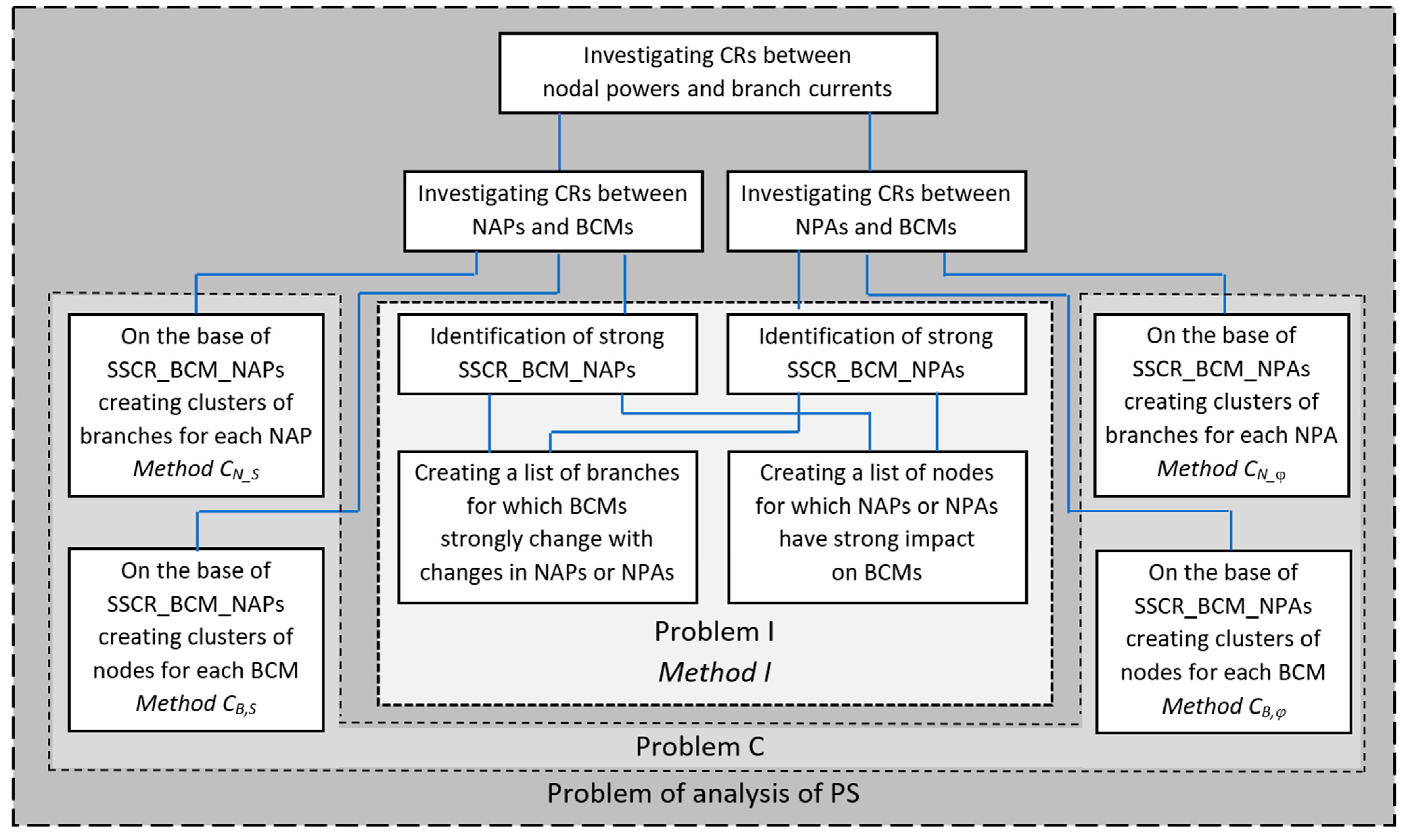
4.2. Methods of Clustering of the PS Based on the Investigation of Correlations Between the Distinguished Quantities

The following methods are proposed to solve Problem C:

• Method C_B,S and Method C_B,φ—methods of clustering of the PS from the point of view of changes in individual BCMs as a consequence of changes in NAPs or NPAs, respectively.
• Method C_{N_S} and Method C_{N_φ}—methods of clustering of the PS from the point of view of changes in individual NAPs or NPAs impacting on changes in BCMs, respectively.

The result of applying Method C_B,S, Method C_B,φ, Method C_{N_S}, or Method C_{N_φ} for i, j, k ∈ {1, 2, …, n} i ≠ j, is cluster $C_{\mathrm{S},\mathrm{I}ij}^{range}$, $C_{\phi ,\mathrm{I}ij}^{range}$, $C_{\mathrm{S}k}^{range}$, or $C_{\phi k}^{range}$, respectively. Elements of each of clusters $C_{\mathrm{S},\mathrm{I}ij}^{range}$ and $C_{\phi ,\mathrm{I}ij}^{range}$ are the nodes of the PS, and elements of each of clusters $C_{\mathrm{S}k}^{range}$ and $C_{\phi k}^{range}$ are the branches of the PS.

Hereinafter:

• If Y ∈ {S, φ}, the following statements will be treated as equivalent: (i) “cluster $C_{Y,\mathrm{I}ij}^{range}$ is associated with the magnitude of the current on branch b_{i_j}” and “cluster $C_{Y,\mathrm{I}ij}^{range}$ is associated with branch b_{i_j}”, and (ii) “cluster $C_{Sk}^{range}$ is associated with the NAP at node n_k”, “cluster $C_{\phi k}^{range}$ is associated with the NPA at node n_k”, and “cluster $C_{Yk}^{range}$ is associated with node n_k”.
• Superscript range denotes interval [th, 1], where th is a constant, limiting, from the bottom, the values of KRCCs of CRs between the quantities that are considered in the case of a cluster. Thus, th can be treated as a parameter of the PS clustering. A th threshold of 0 means that there is no lower bound on the previously mentioned KRCCs.

4.2.1. Method C_B,S

• Step 0–Step 3

Step 0–Step 3 of Method I in the part regarding BCMs and NAPs.

• Step 4

For each BCM I_ij i, j ∈ {1, 2, …, n}, i ≠ j, create set $A_{Y,\mathrm{I}ij}^{range}$ Y = S, i.e., a set of NAPs being in SSCRs with BCM I_ij under the assumption that the absolute value of the KRCC of each mentioned SSCR is within the interval range.

• Step 5

For each BCM I_ij i, j ∈ {1, 2, …, n}, i ≠ j, create set $C_{Y,\mathrm{I}ij}^{range}$ Y = S, i.e., a set of nodes at which there are NAPs in set $A_{Y,\mathrm{I}ij}^{range}$. Set $C_{Y,\mathrm{I}ij}^{range}$ defines the cluster associated with I_ij.

4.2.2. Method C_B,φ

The principle of Method C_B,φ can be obtained by replacing NAPs and Y = S in the description of Method C_B,S by NPAs and Y = φ, respectively.

4.2.3. Method C_{N_S}

• Step 0–Step 3

Step 0–Step 3 of Method I in the part regarding BCMs and NAPs.

• Step 4

For each NAP S_k k ∈ {1, 2, …, n}, create set $A_{\mathrm{S}k}^{range}$, i.e., a set of BCMs being in SSCRs with NAP S_k under the assumption that the absolute value of the KRCC of each mentioned SSCR is within the interval range.

• Step 5

For each NAP S_k k ∈ {1, 2, …, n}, create set $C_{\mathrm{S}k}^{range}$, i.e., a set of branches on which currents have magnitudes in set $A_{\mathrm{S}k}^{range}$. Set $C_{\mathrm{S}k}^{range}$ defines the cluster associated with S_k.

4.2.4. Method C_{N_φ}

The principle of Method C_{N_φ} can be obtained by replacing NAP and S_k in the description of Method C_{N_S} by NPA and φ_k.

5. Case Study 1

This section presents the application of the previously described methods, i.e., Method I, Method C_B,S, Method C_B,φ, Method C_{N_S}, and Method C_{N_φ}. Two test systems are considered, i.e., TS14 and TS30.

5.1. IEEE 14-Bus Test System

For the purposes of the proposed methods, data from TS14 were taken under consideration. States in TS14 were considered in which the system active power losses were in the interval [0.06, 0.34] pu. This part of the investigation is called Case a (Case x, where x = a). The additional superscript a in symbols refers to Case a.

In the analyses, CRs between BCMs and NAPs and between BCMs and NPAs were taken into account separately. In each of these cases, taking into account characteristic CRs for branches, the number of all CRs was equal to 280 (number of nodes: 14, number of branches: 20). In

Table 2. The numbers of SSCRs as a percentage of the total numbers of CRs in Case a.

Quantities in CRs	Number of SSCRs (%)
NAPs, BCMs	34.29
NPAs, BCMs	30.48

, the numbers of SSCRs are shown as a percentage of the total numbers of CRs in the considered cases. Testing the statistical significance of CRs was performed under assumption that the significance level was equal to 0.01.

Table 3. NAPs and BCMs, between which are the SSCRs and KRCCs of these CRs for Case a (TS14).

Sk	Iij	${\mathit{t}}_{\mathbf{k},\mathbf{I}\mathit{i}\mathit{j}-\mathbf{S}\mathit{k}-}^{\mathbf{a}}$	Sk	Iij	${\mathit{t}}_{\mathbf{k},\mathbf{I}\mathit{i}\mathit{j}-\mathbf{S}\mathit{k}-}^{\mathbf{a}}$	Sk	Iij	${\mathit{t}}_{\mathbf{k},\mathbf{I}\mathit{i}\mathit{j}-\mathbf{S}\mathit{k}-}^{\mathbf{a}}$	Sk	Iij	${\mathit{t}}_{\mathbf{k},\mathbf{I}\mathit{i}\mathit{j}-\mathbf{S}\mathit{k}-}^{\mathbf{a}}$	Sk	Iij	${\mathit{t}}_{\mathbf{k},\mathbf{I}\mathit{i}\mathit{j}-\mathbf{S}\mathit{k}-}^{\mathbf{a}}$
S8	l7_8	0.91	S4	l2_5	0.38	S8	l7_9	0.21	S1	l6_11	0.13	S13	l4_7	0.10
S3	l2_3	0.82	S9	l4_7	0.38	S9	l2_4	0.20	S1	l13_14	0.13	S13	l7_9	0.10
S3	l3_4	0.80	S14	l13_14	0.36	S4	l1_2	0.19	S12	l5_6	0.13	S14	l1_5	0.10
S1	l1_2	0.79	S3	l2_4	0.36	S6	l12_13	0.19	S13	l4_9	0.13	S3	l5_6	0.10
S1	l1_5	0.76	S4	l4_5	0.34	S9	l5_6	0.19	S14	l6_12	0.13	S6	l5_6	0.10
S1	l4_5	0.61	S6	l10_11	0.34	S14	l5_6	0.18	S1	l6_12	0.12	S6	l6_12	0.10
S1	l2_3	0.60	S6	l6_11	0.30	S1	l6_13	0.17	S1	l7_9	0.12	S8	l4_5	0.10
S1	l2_4	0.55	S6	l13_14	0.29	S14	l7_9	0.17	S1	l10_11	0.12	S9	l1_2	0.10
S12	l6_12	0.55	S4	l1_5	0.28	S9	l1_5	0.17	S14	l2_4	0.12	S9	l6_13	0.10
S3	l1_2	0.496	S13	l5_6	0.27	S14	l2_5	0.15	S8	l4_7	0.12	S10	l1_5	0.09
S3	l4_5	0.49	S13	l6_12	0.26	S6	l6_13	0.15	S9	l4_5	0.12	S10	l2_5	0.09
S3	l1_5	0.47	S14	l6_13	0.26	S1	l4_7	0.14	S9	l6_11	0.12	S10	l10_11	0.09
S9	l4_9	0.47	S3	l2_5	0.26	S1	l4_9	0.14	S1	l12_13	0.11	S10	l4_7	0.08
S14	l9_14	0.46	S13	l12_13	0.25	S10	l6_11	0.14	S10	l6_12	0.11	S4	l3_4	−0.09
S1	l2_5	0.45	S1	l5_6	0.23	S13	l2_5	0.14	S10	l9_10	0.11	S6	l9_14	−0.11
S13	l6_13	0.44	S14	l4_9	0.23	S13	l9_14	0.14	S13	l1_5	0.11	S13	l10_11	−0.11
S1	l3_4	0.43	S9	l2_5	0.23	S6	l1_5	0.14	S13	l2_4	0.11	S13	l6_11	−0.13
S9	l7_9	0.42	S14	l4_7	0.22	S6	l1_2	0.14	S9	l13_14	0.11	S13	l13_14	−0.19
S4	l2_4	0.40	S14	l12_13	0.21	S9	l10_11	0.14	S10	l5_6	0.10	S12	l12_13	−0.36

The shaded part of the table contains data for SSCRs whose KRCCs have absolute values not less than 0.5.

and

Table 4. NPAs and BCMs, between which are the SSCRs and KRCCs of these CRs for Case a (TS14).

φk	Iij	${\mathit{t}}_{\mathbf{k},\mathbf{I}\mathit{i}\mathit{j}-\phi \mathit{k}-}^{\mathbf{a}}$	φk	Iij	${\mathit{t}}_{\mathbf{k},\mathbf{I}\mathit{i}\mathit{j}-\phi \mathit{k}-}^{\mathbf{a}}$	φk	Iij	${\mathit{t}}_{\mathbf{k},\mathbf{I}\mathit{i}\mathit{j}-\phi \mathit{k}-}^{\mathbf{a}}$	φk	Iij	${\mathit{t}}_{\mathbf{k},\mathbf{I}\mathit{i}\mathit{j}-\phi \mathit{k}-}^{\mathbf{a}}$	φk	Iij	${\mathit{t}}_{\mathbf{k},\mathbf{I}\mathit{i}\mathit{j}-\phi \mathit{k}-}^{\mathbf{a}}$
φ6	l6_11	0.31	φ4	l1_5	0.17	φ13	l13_14	0.09	φ10	l9_10	−0.11	φ9	l6_13	−0.15
φ8	l7_8	0.29	φ6	l6_12	0.16	φ8	l6_11	0.09	φ13	l4_7	−0.11	φ14	l6_13	−0.16
φ4	l2_4	0.26	φ3	l1_5	0.15	φ9	l7_8	−0.08	φ13	l4_9	−0.11	φ9	l10_11	−0.16
φ6	l12_13	0.26	φ9	l4_7	0.13	φ10	l7_9	−0.09	φ13	l9_14	−0.11	φ9	l12_13	−0.16
φ4	l2_5	0.25	φ2	l1_2	0.12	φ12	l5_6	−0.09	φ5	l1_2	−0.11	φ9	l13_14	−0.18
φ6	l10_11	0.25	φ3	l2_4	0.12	φ13	l1_5	−0.09	φ9	l6_12	−0.12	φ9	l6_11	−0.19
φ6	l13_14	0.25	φ8	l2_3	0.12	φ14	l1_5	−0.09	φ13	l2_5	−0.13	φ13	l5_6	−0.2
φ3	l2_3	0.24	φ9	l4_5	0.12	φ9	l3_4	−0.09	φ13	l6_12	−0.13	φ6	l9_14	−0.21
φ6	l6_13	0.24	φ4	l1_2	0.11	φ10	l2_4	−0.1	φ14	l2_5	−0.13	φ13	l6_13	−0.25
φ12	l12_13	0.23	φ8	l3_4	0.11	φ13	l2_4	−0.1	φ14	l5_6	−0.13	φ14	l13_14	−0.25
φ3	l3_4	0.23	φ8	l4_5	0.11	φ13	l7_9	−0.1	φ10	l4_7	−0.14	φ6	l9_10	−0.28
φ4	l4_5	0.22	φ8	l7_9	0.11	φ14	l2_4	−0.1	φ10	l4_9	−0.14	φ14	l9_14	−0.3
φ9	l9_10	0.21	φ6	l1_5	0.1	φ14	l7_9	−0.1	φ13	l12_13	−0.14	φ12	l6_12	−0.34
φ9	l9_14	0.18	φ8	l1_2	0.1	φ5	l1_5	−0.1	φ14	l4_9	−0.14
φ3	l1_2	0.17	φ8	l4_7	0.1	φ10	l2_5	−0.11	φ14	l12_13	−0.14
φ3	l4_5	0.17	φ8	l10_11	0.1	φ10	l5_6	−0.11	φ14	l4_7	−0.15

The shaded parts of the table contain data for SSCRs whose KRCCs have absolute values not less than 0.3.

show the data related to SSCRs, which are members of sets $S_{\mathrm{S},\mathrm{I}-\mathrm{S}}^{\mathrm{a}}$ and $S_{\mathrm{S},\mathrm{I}-\phi }^{\mathrm{a}}$, respectively.

Table 3 and Table 4 show data on the characteristic SSCRs (for branches) between BCMs and NAPs and between BCMs and NPAs, respectively. In the tables, these are also KRCCs in addition to symbols of BCMs, NAPs, or NPAs. In each of the mentioned tables, the data are arranged in the order of decreasing KRCCs.

Based on Table 3, it can be stated that:

$$\begin{gathered} S_{\mathrm{S},\mathrm{I}-\mathrm{S}}^{\mathrm{a},\left[0.5, 1\right]}=\{{\mathrm{c}\mathrm{r}}_{\mathrm{I}7\_8-\mathrm{S}8},{\mathrm{c}\mathrm{r}}_{\mathrm{I}2\_3-\mathrm{S}3},{\mathrm{c}\mathrm{r}}_{\mathrm{I}3\_4-\mathrm{S}3},{\mathrm{c}\mathrm{r}}_{\mathrm{I}1\_2-\mathrm{S}1},{\mathrm{c}\mathrm{r}}_{\mathrm{I}1\_5-\mathrm{S}1}, \\ {\mathrm{c}\mathrm{r}}_{\mathrm{I}4\_5-\mathrm{S}1},{\mathrm{c}\mathrm{r}}_{\mathrm{I}2\_3-\mathrm{S}1},{\mathrm{c}\mathrm{r}}_{\mathrm{I}2\_4-\mathrm{S}1},{\mathrm{c}\mathrm{r}}_{\mathrm{I}6\_12-\mathrm{S}12}, \}, \end{gathered}$$

(14)

$$\begin{gathered} S_{\mathrm{S},\mathrm{I}-\mathrm{S}}^{\mathrm{a},\left[0.3, 1\right]}=S_{S,I-S}^{\left[0.5, 1\right]}\cup \{{\mathrm{c}\mathrm{r}}_{\mathrm{I}1\_2-\mathrm{S}3},{\mathrm{c}\mathrm{r}}_{\mathrm{I}4\_5-\mathrm{S}3},{\mathrm{c}\mathrm{r}}_{\mathrm{I}1\_5-\mathrm{S}3},{\mathrm{c}\mathrm{r}}_{\mathrm{I}4\_9-\mathrm{S}9},{\mathrm{c}\mathrm{r}}_{\mathrm{I}9\_14-\mathrm{S}14}, \\ {\mathrm{c}\mathrm{r}}_{\mathrm{I}2\_5-\mathrm{S}1},{\mathrm{c}\mathrm{r}}_{\mathrm{I}6\_13-\mathrm{S}13},{\mathrm{c}\mathrm{r}}_{\mathrm{I}3\_4-\mathrm{S}1},{\mathrm{c}\mathrm{r}}_{\mathrm{I}7\_9-\mathrm{S}9},{\mathrm{c}\mathrm{r}}_{\mathrm{I}2\_4-\mathrm{S}4},{\mathrm{c}\mathrm{r}}_{\mathrm{I}2\_5-\mathrm{S}4}, \\ {\mathrm{c}\mathrm{r}}_{\mathrm{I}4\_7-\mathrm{S}9},{\mathrm{c}\mathrm{r}}_{\mathrm{I}13\_14-\mathrm{S}14},{\mathrm{c}\mathrm{r}}_{\mathrm{I}2\_4-\mathrm{S}3},{\mathrm{c}\mathrm{r}}_{\mathrm{I}12\_13-\mathrm{S}12},{\mathrm{c}\mathrm{r}}_{\mathrm{I}4\_5-\mathrm{S}4},{\mathrm{c}\mathrm{r}}_{\mathrm{I}10\_11-\mathrm{S}6},{\mathrm{c}\mathrm{r}}_{\mathrm{I}6\_11-\mathrm{S}6}\}, \end{gathered}$$

(15)

Table 4 shows that:

$$S_{\mathrm{S},\mathrm{I}-\phi }^{\mathrm{a},\left[0.5, 1\right]}=\varnothing ,$$

(16)

$$S_{\mathrm{S},\mathrm{I}-\phi }^{\mathrm{a},\left[0.3, 1\right]}=\{{\mathrm{c}\mathrm{r}}_{\mathrm{I}6\_12-\phi 12},{\mathrm{c}\mathrm{r}}_{\mathrm{I}6\_11-\phi 6},{\mathrm{c}\mathrm{r}}_{\mathrm{I}9\_14-\phi 14}\}.$$

(17)

In this and the next sections, when determining the contents of sets $A_{\mathrm{B}}^{\mathrm{a},\left[th, 1\right]}$ and $A_{\mathrm{N}}^{\mathrm{a},\left[th, 1\right]}$, it was assumed that strong CRs were taken into account. Therefore, according to Table 1, th = 0.5. In this situation:

$$A_{\mathrm{B}}^{\mathrm{a},\left[0.5, 1\right]}=\{{\mathrm{b}}_{7\_8}{, \mathrm{b}}_{2\_3}{, \mathrm{b}}_{3\_4}, {\mathrm{b}}_{1\_2}{, \mathrm{b}}_{1\_5}{, \mathrm{b}}_{4\_5}, {\mathrm{b}}_{2\_4}{, \mathrm{b}}_{6\_12}\}.$$

(18)

$$A_{\mathrm{N}}^{\mathrm{a},\left[0.5, 1\right]}=\{{\mathrm{n}}_8,{\mathrm{n}}_3, {\mathrm{n}}_1{,\mathrm{n}}_{12}\}.$$

(19)

Potential CRs between BCMs and NAPs and potential CRs between BCMs and NPAs are symbolically shown in Figure 2 and Figure 3, respectively. The cell at the intersection of a column and a row of the table in Figure 2 symbolizes CRs between BCMs and NAPs that are associated with the mentioned column and row, respectively. Cells in colors other than white symbolize SSCRs. Such cells in column I_ij i, j ∈ {1, 2, …, 14}, i ≠ j (i.e., in the column to which BCM I_ij is associated) indicate NAPs that define cluster $C_{S,\mathrm{I}ij}^{\mathrm{a},[0, 1]}$. At the top of Figure 2, for cluster $C_{S,\mathrm{I}ij}^{\mathrm{a},[0, 1]}$, an avarage of absolute values of KRCCs of SSCRs comprising BCM I_ij is given.

The table in Figure 2 also allows defining clusters $C_{\mathrm{S}k}^{\mathrm{a},[0, 1]}$ k ∈ {1, 2, …, n}. The cells in row S_k (i.e., the row to which NAP S_k is associated) point to BCMs that define cluster $C_{\mathrm{S}k}^{\mathrm{a},[0, 1]}$. On the right side of Figure 2, for cluster $C_{\mathrm{S}k}^{\mathrm{a},[0, 1]}$, an average of absolute values of KRCCs of SSCRs comprising NAP S_k is given.

In Figure 2, SSCRs are distinguished according to the rule of thumb for interpreting the size of KRCCs given in Table 1.

In Figure 2, the table is divided into four areas. AREA 1 and AREA 4 are associated with the higher-voltage part (HVP_TS) of TS14 and the lower-voltage part (LVP_TS) of TS14, respectively. Of the two quantities occurring in SSCRs symbolized by cells in AREA 2 and AREA 3, one of them is associated with HVP_TS and the other is associated with LVP_TS.

Figure 3 applies to SSCRs between BCMs and NPAs. The rules used in Figure 3 are analogous to the rules taken into account in the case of Figure 2.

Analyzing Figure 2 and Figure 3, it can be easily noticed that the number of cluster elements was different for different values of the th parameter. This is shown in Figure 4 for cluster $C_{S1}^{\mathrm{a},[th, 1]}$. The branches marked with colors other than black are elements of cluster $C_{\mathrm{S}1}^{\mathrm{a},[\mathrm{t}\mathrm{h}, 1]}$. The branch colors are applied according to the same principle as that used in Figure 2 and Figure 3. Each of these colors corresponds to the range of KRCC values in which there is KRCC of the characteristic CR between NAP S₁ and the magnitude of current on the branch marked with the considered color.

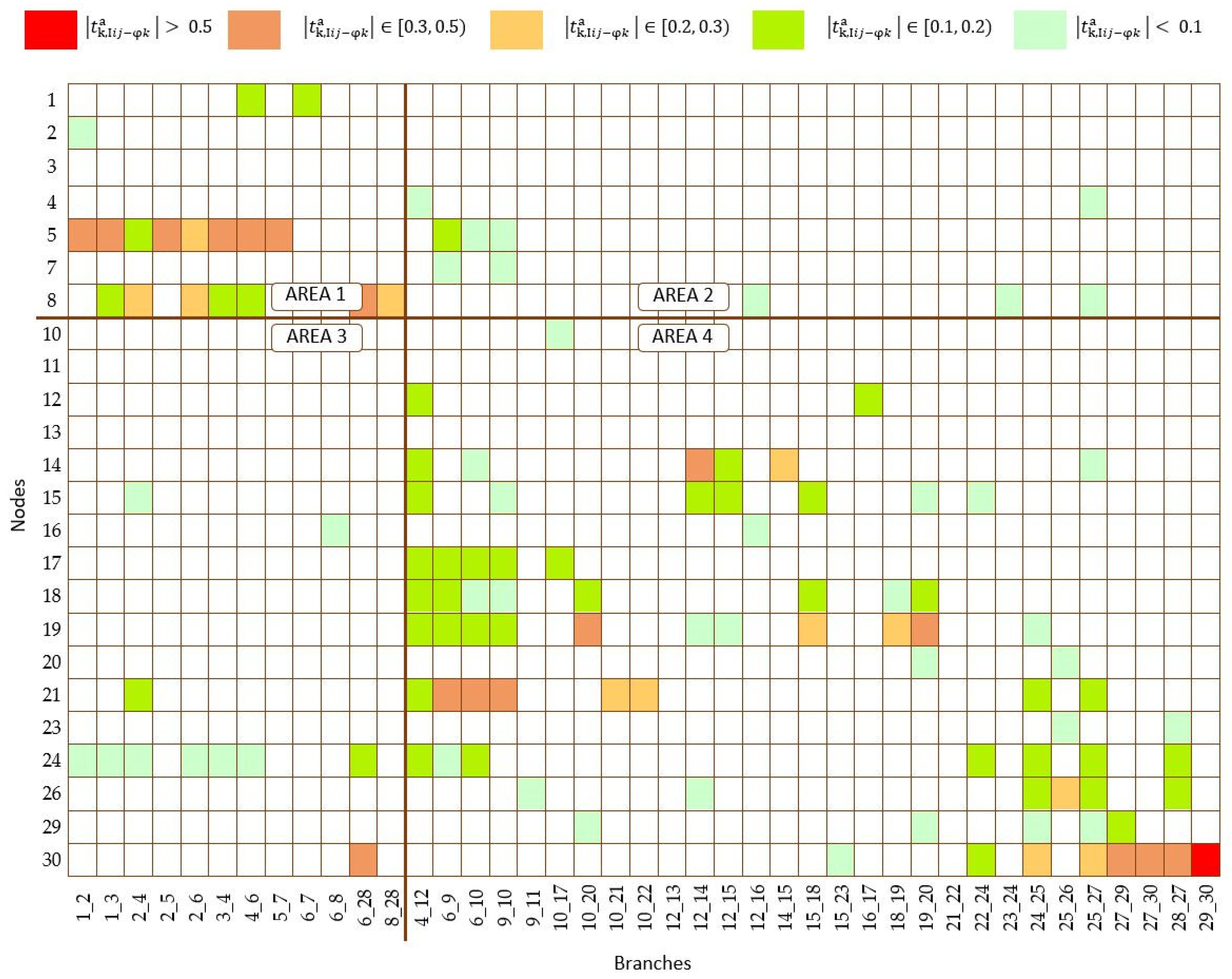
5.2. IEEE 30-Bus Test System

Analogous calculations to those performed for TS14 were performed for TS30.

The calculation results are presented in Figure 5 and Figure 6. The same convention of color-coding SSCRs, whose KRCCs belong to the distinguished value ranges, was used in these figures as in the case of calculations for the IEEE 14-Bus Test System. To increase the readability of the figures, they do not contain (i) NAP or NPA symbols, there are only numbers of nodes at which the nodal powers are considered, (ii) BCM symbols, in place of which the end nodes of the branches are given in the following way: n_i_n_j, where n_i and n_j are the numbers of the end nodes of the considered branch, (iii) KRCC values for SSCRs, and (iv) averages of absolute values of KRCCs of SSCRs comprising a given BCM and, analogously, averages of absolute values of KRCCs of SSCRs comprising a given NAP or NPA.

As in TS14, in TS30 there was HVP_TS and LVP_TS. In Figure 5 and Figure 6, AREA 1 refers to HVP_TS and AREA 4 refers to LVP_TS.

In the case of TS30, the number of SSCRs was equal to 24.09% of all CRs between NAPs and BCMs and 11.99% between NPAs and BCMs.

Sets $A_{\mathrm{B}}^{\mathrm{a},\left[\mathrm{t}\mathrm{h}, 1\right]}$ and $A_{\mathrm{N}}^{\mathrm{a},\left[\mathrm{t}\mathrm{h}, 1\right]}$ were as follows:

$$\begin{gathered} A_{\mathrm{B}}^{\mathrm{a},\left[0.5, 1\right]}=\{{\mathrm{b}}_{9\_11},{\mathrm{b}}_{12\_13},{\mathrm{b}}_{25\_26},{\mathrm{b}}_{6\_8},{\mathrm{b}}_{27\_30},{\mathrm{b}}_{29\_30},{\mathrm{b}}_{1\_2},{\mathrm{b}}_{27\_29},{\mathrm{b}}_{3\_4},{\mathrm{b}}_{1\_3},{\mathrm{b}}_{10\_21}, \\ {\mathrm{b}}_{12\_14},{\mathrm{b}}_{28\_27},{\mathrm{b}}_{10\_22}, {\mathrm{b}}_{19\_20},{\mathrm{b}}_{10\_20},{\mathrm{b}}_{8\_28},{\mathrm{b}}_{6\_7},{\mathrm{b}}_{21\_22}\}, \end{gathered}$$

(20)

$$A_{\mathrm{N}}^{\mathrm{a},\left[0.5, 1\right]}=\{{\mathrm{n}}_{11},{\mathrm{n}}_{13},{\mathrm{n}}_{26},{\mathrm{n}}_8,{\mathrm{n}}_{30},{\mathrm{n}}_1,{\mathrm{n}}_{21},{\mathrm{n}}_{14},{\mathrm{n}}_{19},{\mathrm{n}}_5 \}.$$

(21)

Analyzing the rows as well as the columns in the tables in Figure 5 and Figure 6 allowed us to define the appropriate TS30 clusters.

6. Case Study 2

To investigate the properties of the proposed methods, they were applied for different TS14 loading levels. Case Study 2 was performed only for TS14.

In this section, three cases were considered, namely, Case l, Case m, and Case L, i.e., the cases of low, medium, and large system loads, respectively. These loads were characterized by system active power losses, as given in

Table 5. Characteristics of considered TS14 loading levels.

Interval of System Active Power Losses, pu	TS14 Loading Level
[0.06, 0.13)	low
[0.13, 0.20)	medium
[0.20, 0.27]	large

. The system active power loss intervals for Case l, Case m, and Case L are sub-intervals of the system active power loss interval for Case a. Similarly, as in Case a, the additional superscripts l, m, or L in symbols refer to Case l, Case m, or Case L, respectively.

The results of using the proposed methods for Case l, Case m, and Case L are given in Appendix A, Appendix B, and Appendix C, respectively. In each of those cases, the same procedure was followed as in the case presented in the previous section. The previously mentioned Appendices contain figures analogous to Figure 2 and Figure 3, which concisely present the results of applying the proposed method.

7. Analyses of Results of Case Studies and Discussion

In this section, SSCRs between BCMs and NAPs, as well as SSCRs between BCMs and NPAs, are considered. Hereinafter, SSCR_BCM_NAP stands for the SSCR between BCMs and NAPs, and SSCR_BCM_NPA stands for the SSCR between BCMs and NPAs.

7.1. Taking into Account All Data—General Considerations

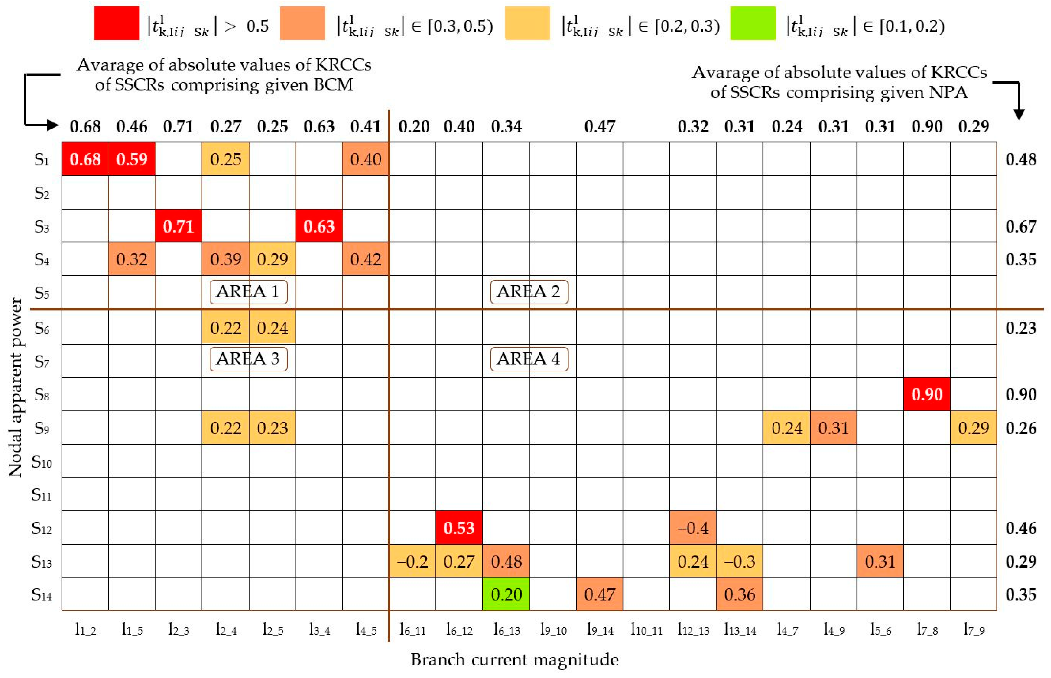
7.1.1. Correlational Relationships Between Branch–Current Magnitudes and Nodal Apparent Powers in the Case of TS14

In Case Study 1 (Case a), with respect to relatively few SSCR_BCM_NAPs (10.53% of the number of all SSCRs), a strong association of the considered quantities (KRCC > 0.5) could be observed. The set of SSCRs for which the KRCC was not less than 0.5 included CRs between:

• NAP S₁ and the magnitudes of the current on the branches that were on the transition paths from node n₁ to all nodes in HVP_TS,
• NAP S₃ and the magnitudes of the current on the branches entering node n₃ (i.e., branches b_{2_3} and b_{3_4}) and on branch b_{1_2} (the KRCC for cr_{I1_2-S3} is near to 0.5), which, together with branch b_{2_3}, constitute the transition path between node n₁ and node n₃,
• NAP S₈ and the magnitude of the current on the only branch connecting node n₈ with the rest of TS14,
• NAP S₁₂ and the magnitude of the current on the branch connecting node n₁₂ with node n₆.

It should be noted that (i) node n₁ is a generation node and (ii) there are reactive power sources at nodes n₃ and n₈. It is worth emphasizing that, in addition to node n₁, node n₂ is also a generating node, and that the sources of reactive power are also at nodes n₆ and n₉. However, NAP at node n₂ does not have SSCRs with BCMs in TS14. In turn, NAPs at nodes n₆ and n₉ occurred in SSCRs with BCMs, but the strength of these CRs was small, and only in a few cases was it medium (in the case of S₆, the number of such SSCRs was equal to 1, and in the case of S₉, to 3).

A different type of node than nodes n₁, n₃, and n₈ is node n₁₂. It is a load node. It is connected to nodes n₆ and n₁₃. It turned out that the average BCM (average power-flow magnitude) I_{6_12} was significantly larger compared to the average BCM I_{12_13}. From the laws describing phenomena in the PS, it follows that the power flow on branch b_{6_12} determined the coverage of the power demand at node n₁₂. This fact was visible in the high KRCC value for relationship cr_{I6_12-S12}.

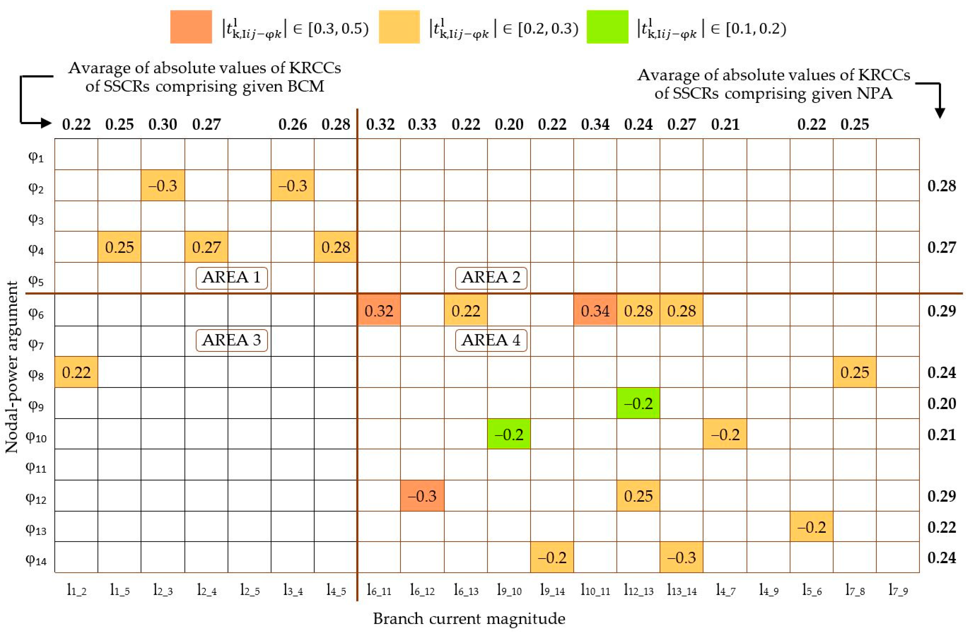
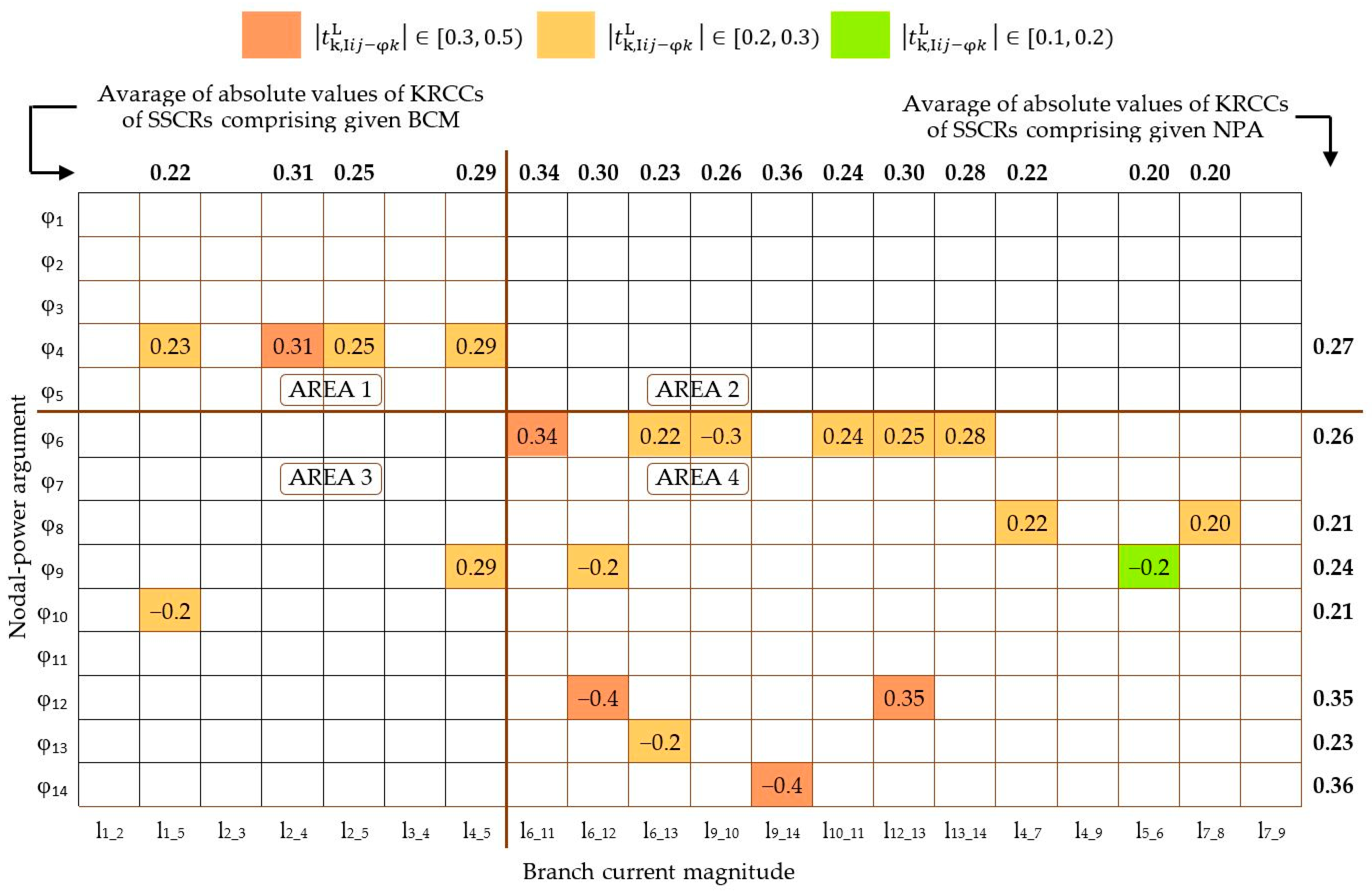
7.1.2. Correlational Relationships Between Branch–Current Magnitudes and the Arguments of Nodal Powers in the Case of TS14

Case Study 1 showed that for TS14, there was no SSCR_BCM_NPAs of which KRCCs had absolute values in the interval [0.5, 1.0]. Moreover, CRs whose KRCCs had absolute values in the interval [0.3, 0.5) were few. There was only one such CR with a positive KRCC and two CRs with negative KRCCs.

Based on the analysis of KRCCs of SSCRs, which are considered in this and the previous point, it can be concluded that NPAs that would be strongly correlated with BCMs could not be found. Also, correlation at the medium level (i.e., when absolute values of KRCCs were in the interval [0.3, 0.5)) was a feature of many more SSCR_BCM_NAPs than SSCR_BCM_NPAs. Therefore, in order to find BCMs that change strongly when the nodal powers change, it is sufficient to take into account SSCR_BCM_NAPs.

7.1.3. Impact of PS Size

For TS30, analogous considerations can be made, such as those given in Section 7.1.1 and Section 7.1.2. It should be noted, however, that in percentage terms, in the case of TS30 there were fewer SSCRs and fewer strong SSCRs. The latter were 8.02% of the number of all SSCRs when SSCR_BCM_NAPs were taken into account. When SSCR_BCM_NPAs were considered, there was one SSCR with KRCCs in the interval [0.5, 1.0], while for TS14 there were no SSCR_BCM_NAPs in this interval.

7.2. Taking into Account Different Parts of the Possessed Data—General Considerations

The number of SSCRs was different for different subsets of the possessed dataset (

Table 6. Numbers of SSCRs between BCMs and NAPs and between BCMs and NPAs for different intervals of system active power losses.

Case x	Interval of System Active Power Losses pu	$\left|{\mathit{S}}_{\mathbf{S},\mathbf{I}-\mathbf{S}}^{\mathit{x}}\right|$	$\left|{\mathit{S}}_{\mathbf{S},\mathbf{I}-\mathbf{S}}^{\mathit{x}}\right|$ %	$\left|{\mathit{S}}_{\mathbf{S},\mathbf{I}-\phi }^{\mathit{x}}\right|$	$\left|{\mathit{S}}_{\mathbf{S},\mathbf{I}-\phi }^{\mathit{x}}\right|$ %
Case a	[0.06, 0.34]	95	100.0	77	100.0
Case l	[0.06, 0.13)	29	30.53	20	25.97
Case m	[0.13, 0.20)	34	35.79	22	28.57
Case L	[0.20, 0.27]	33	34.74	20	25.97

), i.e., for the different intervals of system active power losses (Case x, x = a, l, m, L).

Table 7. Sets $A_{\mathrm{B}}^{x,[0.5,1]}$ and $A_{\mathrm{N}}^{x,[0.5,1]}$, where x = a, l, m, and L in individual TS14 load cases.

Case	Branches	Nodes
Case a	b7_8, b2_3, b3_4, b1_2, b1_5, b4_5, b2_4, b6_12	n8, n3, n1, n12
Case l	b7_8, b2_3, b1_2, b3_4, b1_5, b6_12	n8, n3, n1, n12
Case m	b7_8, b3_4, b2_3, b1_2, b1_5	n8, n3, n1
Case L	b7_8, b3_4, b6_12, b2_3	n8, n3, n12

shows the branches constituting set $A_{\mathrm{B}}^{x,[0.5,1]}$ and the nodes constituting set $A_{\mathrm{N}}^{x,[0.5,1]}$ for different x.

Based on the performed calculations, the following can be concluded:

• Taking into account sets $S_{\mathrm{S},\mathrm{I}-\mathrm{S}}^{\mathrm{l}}, S_{\mathrm{S},\mathrm{I}-\mathrm{S}}^{\mathrm{m}}$, and $S_{\mathrm{S},\mathrm{I}-\mathrm{S}}^{\mathrm{L}},$ one can ascertain that the number of SSCR_BCM_NAPs, for which KRCCs were in the interval [0.5, 1.0], decreased as the TS14 load level increased. In sets $S_{\mathrm{S},\mathrm{I}-\mathsf{\phi }}^{\mathrm{a}}$, $S_{\mathrm{S},\mathrm{I}-\mathsf{\phi }}^{\mathrm{l}}, S_{\mathrm{S},\mathrm{I}-\mathsf{\phi }}^{\mathrm{m}}$, and $S_{\mathrm{S},\mathrm{I}-\mathsf{\phi }}^{\mathrm{L}}$, there was no SSCR for which the KRCC was in the interval [0.5, 1.0].
• Strong SSCRs (i.e., characterized by a KRCC greater than 0.5) observed for smaller amounts of data (Case l, Case m, or Case L) were also observed for larger amounts of data (Case a), but not vice versa. When looking for the most loaded branches in the PS, the largest possible number of PS operating states should be taken into account.
• It should be noted that in none of sets $S_{\mathrm{S},\mathrm{I}-\mathrm{Y}}^{\mathrm{l}}, { S}_{\mathrm{S},\mathrm{I}-\mathrm{Y}}^{\mathrm{m}}$ and $S_{\mathrm{S},\mathrm{I}-\mathrm{Y}}^{\mathrm{L}}$ Y = S, φ were there are any SSCRs for which absolute values of KRCCs were in the interval [0.0, 0.1). Such SSCRs were in sets $S_{\mathrm{S},\mathrm{I}-\mathrm{Y}}^{\mathrm{a}}$ Y = S, φ. The reasons for these facts should be sought in the fact that the number of PS states for which there were data used to determine the strength of CRs, qualified to sets $S_{\mathrm{S},\mathrm{I}-\mathrm{Y}}^{\mathrm{a}}$ Y = S, φ, was much larger than the number of PS states for which there were data used to determine the strength of CRs, qualified to sets $S_{\mathrm{S},\mathrm{I}-\mathrm{Y}}^{\mathrm{l}}, { S}_{\mathrm{S},\mathrm{I}-\mathrm{Y}}^{\mathrm{m}}$ or $S_{\mathrm{S},\mathrm{I}-\mathrm{Y}}^{\mathrm{L}}$ Y = S, φ.
• For the branches on which the currents had magnitudes that strongly changed with changes in NAPs, (i) if they were such in any of the cases Case l, Case m, and Case L, then they were also such in Case a, and (ii) constitute a set with a number of elements decreasing with increasing the load level of TS14 (Table 7).
• The above observation also applied to the nodes at which NAPs strongly affected BCMs.
• Branches b_{7_8}, b_{2_3}, and b_{3_4} were identified as those on which the currents had magnitudes that strongly changed with changes in NAPs regardless of the load level of TS. Two of those branches were connected to node n₃ and one to node n₈. There were reactive power sources in both of the mentioned nodes. It should also be noted that nodes n₃ and n₈ were identified as those nodes at which NAPs strongly affected BCMs regardless of the load level of TS14.

7.3. Clustering of TS14

The results of the TS14 clustering were different for different:

• TS14 load levels (Figure 2, Figure 3 and Figure A1, Figure A2, Figure A3, Figure A4, Figure A5 and Figure A6),
• the th parameter (Figure 4).

In both of the above-mentioned cases, there was a change of (i) the number of clusters, (ii) the cluster sizes, and (iii) the average absolute values of KRCCs of SSCRs, based on which the individual clusters were defined.

In the first case, TS14 clustering was performed based on datasets, each of which referred to different TS14 states. Therefore, different clustering results should be expected, especially since the proposed clustering considers the actual course of phenomena in TS14, which is characterized by the data taken into account.

In the second case, increasing the th parameter limited the number of SSCRs based on which clusters were defined. As a consequence, there may be a decrease in the number of elements in clusters, or even a reduction in the number of clusters. It should be emphasized that these less numerous clusters, with a smaller number of elements, were associated with stronger CRs between the quantities that were considered in clustering.

The elements of clusters associated with branches can be nodes from HVP_TS as well as nodes from LVP_TS. Similarly, the elements of clusters associated with nodes can be branches from both mentioned parts of TS14. The presented observations refer to clusters obtained using Method C_B,S and Method C_{N_S}. In the case of Method C_B,φ and Method C_{N_φ}, the situation was different. The presented observation refers to (i) clusters associated with branches when these branches were in HVP_TS, and (ii) clusters associated with nodes when these nodes were in LVP_TS. It should be noted that the strength of the association of the considered quantities, the CRs of which provide a basis for inserting a node into clusters in the first case and a branch in the second case, when this node or branch is in a different part of TS14 than the branch or node with which the cluster is associated, respectively, is very small or close to very small (Table 1). The presented remark can be justified by the fact that (i) NPAs had the strongest impact on the parts of TS14 closest to the nodes at which these NPAs existed, (ii) in general, the impact of NPAs on TS14 was weak, and (iii) the impact of NPAs on further parts of TS14, in particular on a different part of TS14 than the one in which the mentioned nodes existed, was so weak that in the vast majority of cases, it was statistically insignificant.

In the case of each cluster obtained using Method C_B,S and Method C_{N_S}, if th = 0.5, then nodes or branches constituting this cluster and the branch or the node associated with the mentioned cluster, respectively, were in the same part of TS14. This fact can be justified in the same way as it was done with respect to the remark given earlier. It should be emphasized that the previous justification concerns the case when th = 0, while currently th = 0.5. However, NAPs still had the strongest effect on the parts of TS14 closest to the nodes at which they existed. As we moved away from these nodes, the KRCCs of the corresponding SSCRs became smaller and smaller and, correspondingly, far from the considered nodes, they were smaller than 0.5.

7.3.1. Clustering of PS from the Point of View of Changes in Individual BCMs as a Consequence of Changes in NAPs or NPAs—Method C_B,S and Method C_B,φ

Assuming that th = 0, we can state the following:

• Analyzing Figure 2 and Figure 3, it can be stated that for each branch b_{i_j} i,j ∈ {1, 2, …, 14} i ≠ j, there were clusters $C_{\mathrm{S},\mathrm{I}ij}^{\mathrm{a},[0, 1]}$ and $C_{\phi ,\mathrm{I}ij}^{\mathrm{a}, [0, 1]}$ that were associated with it. This was not the case for Case l, Case m, and Case L.
• Among clusters $C_{\mathrm{S},\mathrm{I}ij}^{\mathrm{a},[0, 1]}$ i,j ∈ {1, 2, …, 14} i ≠ j, two clusters stood out from the others. They were $C_{\mathrm{S},\mathrm{I}9\_10}^{\mathrm{a},[0, 1]}$ and $C_{\mathrm{S},\mathrm{I}7\_8}^{\mathrm{a},[0, 1]}$. Each of these clusters contained one node. It can be seen that:
  • Branches b_{9_10} and b_{10_11} were branches on the transition path from node n₉ to node n₁₁. BCM I_{9_10} differed relatively little from I_{10_11}.
  • Branch b_{7_8}, which was the only branch connecting node n₈ with the rest of the TS14, entered node n₇, with which branches b_{4_7} and b_{7_9} were incident. Branches b_{4_7} and b_{7_9} constituted the transition path between nodes n₄ and n₉. The difference between BCMs I_{4_7} and I_{7_9} was also small.

Such observations could not be made for other branches.

3.

If TS14 clustering was performed using Method C_B,S, then in Case a, the elements of the clusters associated with any branch in HVP_TS were nodes n₁ and n₃, and if branch b_{2_3} was omitted, then n₄ was also such an element. It should be noted that n₁ is a generation node and n₃ is a node with a reactive power compensator. Node n₄ is on the higher-voltage side of the transformer, being between HVP_TS and LVP_TS. There is no such node that is an element of every cluster associated with any branch in LVP_TS.

7.3.2. Clustering of PS from the Point of View of Changes in Individual NAPs or NPAs Impacting on Changes in BCMs—Method C_{N_S} and Method C_{N_φ}

Analysis of clusters defined by Method C_{N_S} allowed us to conclude that:

• Regardless of the TS14 load level, Method C_{N_S} did not provide a basis for defining clusters associated with nodes n₂, n₅, and n₇. This is due to the fact that each of NAPs S₂, S₅, and S₇ did not enter any SSCR. It should be emphasized that node n₇ is an internal node of the three-winding transformer model and, as such, was not taken into account in the analyses that were carried out here. NAPs at nodes n₂ and n₅ did not have a significant impact on BCMs in TS14. The NAP at node n₂ reached relatively high values, but in a significant number of operating states of TS14 it was lower than NAPs at nodes n₁ and n₃ simultaneously. Nodes n₁ and n₃ are neighboring nodes to node n₂. In turn, in almost all operating states of TS14, the NAP at node n₅ was lower than the NAPs at any neighboring node.
• In Case a, cluster $C_{\mathrm{S}1}^{\mathrm{a},[0, 1]}$ included the largest number of branches (17 branches). Next were $C_{\mathrm{S}13}^{\mathrm{a},[0, 1]}$ (14 branches) and $C_{\mathrm{S}9}^{\mathrm{a},[0, 1]}$ (13 branches). Cluster $C_{\mathrm{S}1}^{\mathrm{a},[0, 1]}$ was also distinguished by the number of branches on which currents had magnitudes remaining in strong SSCRs with NAP S₁ (see Table 1). In this respect, the next node was node n₃, then n₈ and n₁₂. In Case l and Case m, the cluster associated with node n₁ was no longer in first place in the discussed ranking, appearing in second place, with the same number of considered branches as the cluster associated with node n₃, but worse characteristics of the considered SSCRs. In Case L, the cluster associated with node n₁ no longer had the branches with currents having magnitudes remaining in strong SSCRs with NAP S₁. Cluster $C_{\mathrm{S}3}^{\mathrm{a},[0, 1]}$ did not have a very large number of branches. The branches of cluster $C_{\mathrm{S}3}^{\mathrm{a},[0, 1]}$ were mostly in HVP_TS. The numbers of branches in clusters $C_{\mathrm{S}8}^{\mathrm{a},[0, 1]}$ and $C_{\mathrm{S}12}^{\mathrm{a},[0, 1]}$ should be considered small. These branches were located primarily in LVP_TS. The clusters associated with nodes n₃, n₈, and n₁₂ retained their importance regardless of the TS14 load level. The importance of a cluster was assessed based on the branches belonging to it that contained currents with magnitudes that were in strong SSCRs.
  In Section 7.1.1, the importance of nodes n₁, n₃, n₈, and n₁₂ in TS14 was discussed. The earlier-presented facts are a logical consequence of this importance.

Considering the properties of clusters defined by Method C_{N_φ}, we observed the following:

• Regardless of the TS14 load level, Method C_{N_φ} did not provide a basis for defining clusters associated with nodes n₁, n₇, and n₁₁. The lack of a cluster associated with n₁ resulted from the fact that it is the slack node. The case of node n₇ was described earlier. NPAs at node n₁₁ did not have a significant impact on BCMs in TS14. CRs with NPA φ₁₁ were not SSCRs and, therefore, there was no basis for defining the cluster associated with node n₁₁.
• In Case a, cluster $C_{\phi 9}^{\mathrm{a},[0, 1]}$ included the most branches. The same number of branches was found in cluster $C_{\phi 13}^{\mathrm{a},[0, 1]}$. Considering the number of branches, the next clusters to be mentioned were $C_{\phi 14}^{\mathrm{a},[0, 1]}$, $C_{\phi 6}^{\mathrm{a},[0, 1]}$, and $C_{\phi 8}^{\mathrm{a},[0, 1]}$. The greater part of the branches of each of the mentioned clusters was in LVP_TS. The clusters including a smaller number of branches were $C_{\phi 3}^{\mathrm{a},[0, 1]}$ and $C_{\phi 4}^{\mathrm{a},[0, 1]}$. These clusters were entirely in HVP_TS. It should be noted that nodes n₉, n₆, n₈, and n₃ were at important points of TS14. Nodes n₉ and n₆ were on the only transition paths between HVP_TS and LVP_TS on the LVP_TS side. Nodes n₆, n₈, and n₃ are nodes with reactive power compensators. Nodes n₁₃ and n₁₄ are load nodes. In each of them, the average NAP was greater than the average NAP in every other node in LVP_TS except nodes n₆ and n₉.
  In Case l, Case m, and Case L, the clusters defined by Method C_{N_φ} had sizes significantly different from those in Case a. When the TS14 load level changed, the cluster that stood out the most was the cluster associated with node n₆. It had a relatively large size (the largest in comparison to other clusters) and changed little with changes in the TS14 load level. This means that NPA φ₆ had a significant effect on BCMs regardless of the TS14 load level.

8. Conclusions

Knowledge of power flows in the PS is essential for its proper exploitation and for recognizing development needs. It is the starting point for many analyses. This paper allowed us to increase knowledge in the field of power flows in the PS. It provided new methods of PS analysis based on data mining. The proposed methods were (i) the method of identifying PS branches, on which currents had magnitudes that strongly changed when magnitudes or arguments of nodal powers changed, and identifying the nodes at which these powers existed, and (ii) methods of PS clustering using statistically significant correlation relationships between magnitudes and arguments of nodal powers and branch current magnitudes.

The developed PS clustering methods allowed for defining clusters in two ways. The first one led to clusters, each of which included nodes, at which nodal powers had magnitudes or arguments statistically significantly correlated with the magnitude of the current on a certain branch. The second way of determining clusters assumed that each cluster included branches, on which currents had magnitudes, being statistically significantly correlated with the magnitude or argument of nodal power at a certain node.

The summary of the considerations presented in this paper is shown in Figure 7. This figure shows the problems that were considered in the paper and the main ideas for their solutions. These ideas were used in the proposed methods.

Applying the proposed methods to data from TS14, corresponding to all considered TS14 states, and to subsets of the previously mentioned dataset showed that the results in each of the considered cases were different. However, it can be observed that strong CRs between BCMs and NAPs for the mentioned subsets were also indicated for the entire dataset.

An interesting aspect of the TS14 research was the analysis of the strength of CRs between BCMs and NAPs in comparison to the strength of CRs between BCMs and NPAs. It turned out that in general, the strength of CRs between BCMs and NAPs was significantly greater than the strength of CRs between BCMs and NPAs. The absolute values of KRCCs for CRs between BCMs and NPAs were never greater than 0.5 and rarely reached values slightly greater than 0.3.

Applying the developed identification method to TS14, it turned out that it was possible to indicate such situations in which when NAPs at certain nodes changed, (i) the magnitudes of the currents flowing on the branches on the certain energy-flow path changed significantly, and (ii) the significant change occurred in the magnitude of current on the branch on which the power flow was dominant from the point of view of the branches related to the considered node. The method also allowed us to point out the intuitively obvious fact that changes in the magnitude of the current on the only branch entering a given node were strongly related to changes in the NAP at this node.

For a larger system, the number of SSCRs relative to all possible CRs was smaller. However, studies performed for all considered PS states showed that also for a larger PS, the observations given earlier were still valid.

The proposed clustering methods allowed us to gain knowledge about the PS areas in which, on the one hand, there were noticeable relationships between individual nodal powers and branch currents and, on the other hand, there were noticeable relationships between individual branch currents and nodal powers. An additional advantage of the proposed approach is that the strength of the aforementioned relationships can be quantitatively assessed.

Analyzing the properties of the developed methods, it can be concluded that the following properties were common to them: (i) they do not require the implementation of complex calculations and, therefore, do not require the involvement of large computational resources, (ii) they do not require simplifications of the PS model, (iii) they assume the use of only measurement data without the need to have PS parameters, and (iv) the size of the PS is not a limitation for their use.

The results of the developed methods can be used for various PS analyses. In particular, they can be useful for PS planning, as well as for operational management. Attention should also be paid to the investigation of CRs between BCMs and NAPs and between BCMs and NPAs for the aim of the analysis of PSs with distributed generation, which depends on weather factors. In this case, the strength of CRs between BCMs and NAPs, but also the strength of CRs between BCMs and NPAs, can change during the day. This information can be useful for operation purposes.

References

1. Saric, A.T.; Stankovic, A.M. Model uncertainty in security assessment of power systems. IEEE Trans. Power Syst. 2005, 20, 1398–1407. [Google Scholar] [CrossRef]
2. Stewart, G.W.; Sun, G.J. Matrix Perturbation Theory; Academic Press, Inc.: Boston, MA, USA, 1990. [Google Scholar]
3. Jiang, X.; Chen, Y.C.; Domínguez-García, A.D. A set-theoretic framework to assess the impact of variable generation on the power flow. IEEE Trans. Power Syst. 2013, 28, 855–867. [Google Scholar] [CrossRef]
4. Zhang, X.; Chen, Y.L.; Wang, Y.X.; Ding, R.; Zheng, Y.; Wang, Y.; Cheng, X.; Zha, X. Reactive Voltage Partitioning Method for the Power Grid With Comprehensive Consideration of Wind Power Fluctuation and Uncertainty. IEEE Access 2020, 8, 124514–124525. [Google Scholar] [CrossRef]
5. Cichosz, P. Data Mining Algorithms: Explained Using R; John Wiley & Sons: Chichester, UK, 2015. [Google Scholar]
6. Maimon, O.; Rokach, L. Data Mining and Knowledge Discovery, 2nd ed.; Springer: New York, NY, USA, 2010. [Google Scholar]
7. Li, H.; Wang, J. From Soft Clustering to Hard Clustering: A Collaborative Annealing Fuzzy c-Means Algorithm. IEEE Trans. Fuzzy Syst. 2024, 32, 1181–1194. [Google Scholar] [CrossRef]
8. Yin, H.; Aryani, A.; Petrie, S.; Nambissan, A.; Astudillo, A.; Cao, S. A Rapid Review of Clustering Algorithms. arXiv 2024, arXiv:2401.07389v1. [Google Scholar]
9. Rajabi, A.; Eskandari, M.; Ghadi, M.J.; Li, L.; Zhang, J.; Siano, P. A Comparative Study of Clustering Techniques for Electrical Load Pattern Segmentation. Renew. Sustain. Energy Rev. 2020, 120, 109628. [Google Scholar] [CrossRef]
10. Teichgraeber, H.; Brandt, A.R. Clustering Methods to Find Representative Periods for the Optimization of Energy Systems: An initial Framework and Comparison. Appl. Energy 2019, 239, 1283–1293. [Google Scholar] [CrossRef]
11. Rocchetta, R. Enhancing the Resilience of Critical Infrastructures: Statistical Analysis of Power Grid Spectral Clustering and Post-Contingency Vulnerability Metrics. Renew. Sustain. Energy Rev. 2022, 159, 112185. [Google Scholar] [CrossRef]
12. Okon, T.; Wilkosz, K. Diagnostics of reactive power flow in a power network. In Proceedings of the International Conference on Diagnostics in Electrical Engineering (Diagnostika), Pilsen, Czech Republic, 4–7 September 2018; pp. 1–4. [Google Scholar]
13. Kosmala Neto, M.; Okon, T.; Wilkosz, K. Areas of Impact of Nodal Powers on Power Flows in a Power System. In Proceedings of the 24th International Scientific Conference on Electric Power Engineering (EPE), Kouty nad Desnou, Czech Republic, 15–17 May 2024; pp. 1–5. [Google Scholar]
14. Power Systems Test Case Archive, 14 Bus Power Flow Test Case. Available online: https://labs.ece.uw.edu/pstca/pf14/pg_tca14bus.htm (accessed on 25 May 2025).
15. Power Systems Test Case Archive, 30 Bus Power Flow Test Case. Available online: https://labs.ece.uw.edu/pstca/pf30/pg_tca30bus.htm (accessed on 25 May 2025).
16. Trochim, W.M.; Donnelly, J.P.; Arora, K. Research Methods: The Essential Knowledge Base; Cengage Learning, Inc.: Boston, MA, USA, 2014. [Google Scholar]
17. Okon, T.; Wilkosz, K. Propagation of Voltage Deviations in a Power System. Electronics 2021, 10, 949. [Google Scholar] [CrossRef]
18. Okon, T.; Wilkosz, K. Analysis of the Influence of Nodal Reactive Powers on Voltages in a Power System. Energies 2023, 16, 1567. [Google Scholar] [CrossRef]
19. Tao, S.; Xu, Q.; Peng, Y.; Xiao, X.; Tang, N. Correlation between injected power and voltage deviation at the integrating node of new energy source. In Proceedings of the 2nd International Conference on Artificial Intelligence, Management Science and Electronic Commerce (AIMSEC), Dengfeng, China, 8–10 August 2011; pp. 7031–7034. [Google Scholar]
20. Yang, X.; Song, D.; Liu, D.; Wang, F. Node grouping for low frequency oscillation based on Pearson correlation coefficient and its application. In Proceedings of the 2016 IEEE International Conference on Power System Technology (POWERCON), Wollongong, NSW, Australia, 28 September–1 October 2016; pp. 1–5. [Google Scholar]
21. Zuo, J.; Xiang, M.; Zhang, B.; Hen, D.C.; Guo, H. Correlation data analysis for low-frequency oscillation source identification. In Proceedings of the 2017 4th International Conference on Systems and Informatics (ICSAI), Hangzhou, China, 11–13 November 2017; pp. 1466–1470. [Google Scholar]
22. Chmielowiec, K.; Wiczynski, G.; Rodziewicz, T.; Firlit, A.; Dutka, M.; Piatek, K. Location of power quality disturbances sources using aggregated data from energy meters. In Proceedings of the 12th International Conference and Exhibition on Electrical Power Quality and Utilisation (EPQU), Cracow, Poland, 14–15 September 2020; pp. 1–5. [Google Scholar]
23. Feng, D.; Zhou, S.; Wang, T.; Li, Y.; Liu, Y. A method for identifying major disturbance sources in a regional grid. In Proceedings of the IEEE International Power Electronics and Application Conference and Exposition (PEAC), Shenzhen, China, 4–7 November 2018; pp. 1–6. [Google Scholar]
24. Sprent, P.; Smeeton, N.C. Applied Nonparametric Statistical Methods, 3rd ed.; Chapman & Hall/CRC: New York, NY, USA, 2001. [Google Scholar]
25. Gibbons, J.D.; Chakraborti, S. Nonparametric Statistical Inference, 4th ed.; Revised and Expanded; Marcel Dekker, Inc.: New York, NY, USA, 2003. [Google Scholar]
26. Cohen, J. Statistical Power Analysis for the Behavioral Sciences, 2nd ed.; LEA: New York, NY, USA, 1988. [Google Scholar]
Figure 1. The assumed Π model of power line bi_j: zij = rij + j xij, yij = j 0.5 bij, and yji = j 0.5 bij.
Energies 18 03188 g001
Figure 2. SSCRs between BCMs and NAPs for TS14 in Case a.
Energies 18 03188 g002
Figure 3. SSCRs between BCMs and NPAs for TS14 in Case a.
Energies 18 03188 g003
Figure 4. Cluster C S 1 a , [ t h ,   1 ] for TS14 in Case a for (a) th = 0, (b) th = 0.2, and (c) th = 0.5.
Energies 18 03188 g004
Figure 5. SSCRs between BCMs and NAPs for TS30 in Case a.
Energies 18 03188 g005
Figure 6. SSCRs between BCMs and NPAs for TS30 in Case a.
Energies 18 03188 g006
Figure 7. The problems considered in the paper and the methods of their solutions.
Energies 18 03188 g007