Improvement of Wild Horse Optimizer Algorithm with Random Walk Strategy (IWHO), and Appointment as MLP Supervisor for Solving Energy Efficiency Problem

Abstract

This paper aims to enhance the success of the Wild Horse Optimization (WHO) algorithm in optimization processes by developing strategies to overcome the issues of stuckness and early convergence in local spaces. The performance change is observed through a Multi-Layer Perceptron (MLP) sample. In this context, an advanced Wild Horse Optimization (IWHO) algorithm with a random walking strategy was developed to provide solution diversity in local spaces using a random walking strategy. Two challenging test sets, CEC 2019, were selected for the performance measurement of IWHO. Its competitiveness with alternative algorithms was measured, showing that its performance was superior. This superiority is visually represented with convergence curves and box plots. The Wilcoxon signed-rank test was used to evaluate IWHO as a distinct and powerful algorithm. The IWHO algorithm was applied to MLP training, addressing a real-world problem. Both WHO and IWHO algorithms were tested using MSE results and ROC curves. The Energy Efficiency Problem dataset from UCI was used for MLP training. This dataset evaluates the heating load (HL) or cooling load (CL) factors by considering the input characteristics of smart buildings. The goal is to ensure that HL and CL factors are evaluated most efficiently through the use of HVAC technology in smart buildings. WHO and IWHO were selected to train the MLP architecture, and it was observed that the proposed IWHO algorithm produced better results.

1. Introduction

Optimization involves a series of tasks that employ mathematical or analytical methods to enhance the parameters of a given system or process at reduced cost. This process follows a trajectory that enables the problem to attain a global optimum [1]. To date, optimization has been applied to real-world problems represented by mathematical models to address challenges in engineering, finance, and science [2,3]. The development of optimization algorithms has garnered significant interest in addressing optimization issues across various domains, including engineering, science, economics, and business [4,5,6]. A real-world optimization problem can be resolved if it is mathematically expressed. When addressing real-world challenges, it is crucial to optimally derive the desired variables. Consequently, intelligent algorithms have been acknowledged as vital tools for solving these problems. These algorithms are categorized into deterministic and stochastic types [7]. However, deterministic algorithms present several limitations, such as the necessity for complex mathematical computations, implementation challenges, and tendency to become trapped in local optima [2,8]. Stochastic algorithms that employ non-deterministic derivative-free methods have been utilized to mitigate these limitations. In this regard, metaheuristic optimization techniques, classified as stochastic algorithms, provide promising solutions to fulfil this requirement.

Such algorithms are based on theorems derived from scientific laws and mathematical modelling with specific constraints, as well as theorems that mimic the behavior of swarms with shared intelligence [2]. The goal of metaheuristics is to identify search or optimization methods that are superior when applied to instances of a given class of problems. In all swarm-based optimization algorithms, the problem is optimized using a set of random solutions. Each time the algorithm is executed, this set of random solutions is evaluated and improved by using a fitness function. The probability of obtaining an overall optimal solution was increased through enough random solutions and iterations.

Metaheuristic algorithms are characterized by two primary phases: exploration and exploitation. The efficacy of the balance between these phases indicated the overall quality of the algorithm. Exploration pertains to the algorithm’s capacity to survey the entire search space, whereas exploitation involves each search agent’s ability to identify the optimal solution within its local vicinity. The effectiveness of an algorithm in addressing a specific problem set may not necessarily translate to optimization problems of a different nature or type [9]. It is acknowledged that no single optimization algorithm is universally applicable to all problems. Metaheuristic algorithms can be designed to efficiently navigate the search space and deliver optimal solutions within a reasonable time frame.

The Genetic Algorithm (GA) [10] is among the earliest swarm-based algorithms. The particle swarm optimization (PSO) algorithm [11] has been extensively examined and has drawn inspiration from various algorithms, including the Grey Wolf Algorithm (GWO) [12] and Harris Hawks Optimizer (HHO) [8], among others, in terms of their operational principles [11]. The hunger game search algorithm (HGS) [13] was inspired by the hunger drive of animals, a common theme in swarm-based algorithms. Over the past two decades, numerous algorithms have been developed and implemented in this domain [14,15,16].

The No-Free Lunch (NFL) theorem underscores the importance of leveraging problem-specific knowledge to enhance performance, thereby providing an opportunity to develop various strategies for fine-tuning a metaheuristic algorithm as desired [17]. Hybridization techniques can be employed to obtain superior solutions [18,19]. Hybridization offers three significant advantages: it capitalizes on the flexibility of metaheuristics to tackle large-scale problems that individual metaheuristics alone cannot manage by integrating different strategies or algorithms, and it improves the problem-solving performance, resulting in more robust algorithms [20].

Some examples of hybridization were examined in this study.

The authors of one paper highlight that hybrid metaheuristic algorithms improve the effectiveness of individual algorithms by combining their unique advantages. Many hybrid algorithms have been created for feature selection, with the goal of identifying the best feature subsets from datasets. These methods avoid getting stuck in local optima and prevent early convergence while thoroughly examining the search space. The algorithms strike a balance between exploration and exploitation. The improved algorithms produce results that are nearly optimal. By integrating multiple methods, hybrid metaheuristics enhance both convergence and the quality of solutions [21].

The seminal study on hybridization explores hybrid meta-heuristic algorithms for optimizing the dimensions of hybrid renewable energy systems (HRES). HRES enhances energy sustainability in remote areas; however, optimization is complex due to multiple factors. Hybrid meta-heuristic algorithms yield more precise results than traditional methods for HRES optimization. The paper reviews these algorithms for both single-objective and multi-objective design optimization. In single-objective optimization, algorithms such as GA-TS, PSO-HS, and the GA-Markov model are employed to minimize costs and enhance reliability. For multi-objective optimization, algorithms like FPA-SA, MOPSO-NSGA-II, and ACO-ABC are utilized to optimize cost, emissions, and reliability simultaneously. Low-level co-evolutionary hybridization is most commonly employed to balance algorithm exploration and exploitation. The authors note an increased use of hybrid algorithms for multi-objective HRES optimization [22]. The study evaluates an autonomous green energy system using hybrid metaheuristic methods. It presents a hybrid renewable energy system (HRES) with wind turbines, solar photovoltaic panels, biomass gasifier, and fuel cells with hydrogen storage for an off-grid university campus in Turkey. The research examines electricity production and optimization algorithms to minimize annual system cost while ensuring reliable supply. Using a Hybrid Firefly Genetic Algorithm (HFGA), which outperforms other algorithms, the optimal sizing is determined. The standalone system proves most cost-effective, achieving 100% renewable energy fraction [23].

Recently, metaheuristic algorithms have been widely employed to address real-world problems, with applications spanning engineering challenges [24,25], efficient use of air conditioning technology [25], and training of artificial neural networks [2]. Furthermore, a substantial body of literature exists on the integration of metaheuristics into machine learning algorithms [26,27].

For instance, in one study, the authors examined the HVAC system [28]. In paper, introduces a hybrid model that combines physical system modeling with symbolic regression, noted for its effectiveness with limited data and physical expressiveness. This model has been tested on air conditioning systems to forecast energy performance. IWHO develops optimization algorithms for machine learning (MLP) training. The algorithm’s optimization effectiveness and its impact on MLP training are evaluated, with applications to standard optimization tests and MLP training using the UCI Energy Efficiency dataset. IWHO excels in optimization and training stability. Enhanced with a Random Walk strategy, IWHO addresses premature convergence issues and delivers superior results compared to classical WHO and meta-heuristic algorithms, as validated by the Wilcoxon test. As an MLP training consultant, IWHO achieves lower error rates and higher explanatory power (R²: 0.98) than classical WHO, providing precise outcomes in energy efficiency and HVAC systems. Box plots and convergence curves demonstrate that IWHO yields more stable results near the global optimum. Although it is slower by 23%, its accuracy makes this acceptable. IWHO’s adaptable nature suits various optimization problems and machine learning applications, ranging from energy efficiency to engineering design. The algorithm’s primary advantages are its novel optimization approach, integration with machine learning, and successful application to energy efficiency, with statistically significant results and stable performance.

In this study, the IWHO algorithm was utilized as an advisor for an artificial neural network, a machine-learning algorithm, thereby contributing to this field. The wild horse optimization algorithm considered in this study is a swarm-based algorithm [27]. The group hierarchy in a swarm of wild horses is inspired by common swarm behaviors such as the satisfaction of motives. Several studies have addressed the WHO algorithm. It is pertinent to provide examples of previous studies. In 2022, the Wild Horse Optimizer (WHO) algorithm was developed based on swarm characteristics and the hierarchy of wild horses. For instance, to augment the exploitation capacity of the WHO algorithm and prevent it from becoming trapped in local optima, a random running strategy (RRS) was employed to ensure a balance between exploration and exploitation, and to strengthen competition with the waterhole mechanism (CWHM). In addition, the dynamic inertia weight strategy (DIWS) was used to achieve a global optimal result [29]. To address the limitations of the WHO algorithm, such as its inadequate search accuracy and slow convergence speed, a Hybrid Multi-Strategy Improved Wild Horse Optimizer (HMSWHO) is proposed. The Halton sequence is utilized to increase the diversity of the swarm, the adaptive parameter TDR is employed for exploration-exploitation balance, and the simplex method is applied to improve the worst position of the swarm [30]. In another study aimed at enhancing the WHO algorithm, a new algorithm was developed by implementing two strategies to increase the global search efficiency and avoid local optima. The first strategy is the quantum acceleration strategy, which enhances the individual abilities of each horse, and the chaotic mapping strategy, which prevents entrapment in the local optima [31].

Numerous studies have applied the WHO algorithm to various engineering challenges. In one study, the WHO algorithm was employed as a controller in a wind turbine system to standardize the wind speed through a specific controller and to avert potential failures [32]. Another study hybridized the WHO algorithm with the dwarf mongoose optimization (DMO) algorithm to assess its efficacy as a controller to reduce electricity costs in a small-grid system model [33]. Within the domain of energy engineering, the WHO algorithm has demonstrated its effectiveness as an optimization controller [34]. It has also been used for attribute selection [35]. In the context of scheduling problems, the WHO algorithm has been successfully applied to the planning of work processes in workshops by hybridizing it with various strategies [36]. The stability of the WHO algorithm served as a key motivation for this study. The quality of the algorithm was evaluated using the CEC 2019 [37] benchmark functions and hybridized with the Random Walking (RW) strategy to enhance outcomes. The RW strategy augments the potential of metaheuristic algorithms by introducing randomness into local search processes and generating alternative solutions [38,39]. The findings of this study indicated a significant improvement in the performance of the WHO algorithm across most functions. Previously, Eker et al. conducted a similar investigation using the RW-ARO algorithm, which resulted from the hybridization of the artificial rabbit optimization (ARO) algorithm and RW strategy, achieving successful results in Control Engineering [40]. In this study, the proposed IWHO hybrid algorithm was employed to train the CL and HL for HVAC systems in buildings via MLP, with the IWHO designated as the trainer. The WHO algorithm was selected as an alternative. This study utilized the Energy Efficiency dataset from the UCI, which addresses the energy efficiency problem [41]. Previous studies have explored related topics. One study assessed the predictive capabilities of Artificial Neural Networks (ANN) and XGBoost surrogate models for heating, cooling, lighting loads, and equivalent primary energy requirements, using EnergyPlus (Matlab2024) simulation data across various office cell model versions. The XGBoost models exhibited superior accuracy in predicting these loads. The mc-intersite-proj-th sampling method slightly enhanced prediction accuracy compared to maximin Latin hypercube sampling for both models. XGBoost models, which consist of collections of piecewise constant functions, perform optimally when the simulated loads show minimal variation or smaller gradients across the design space. This implies that fewer regression trees may suffice for precise predictions, or the same number could yield more accurate results. In this case study, XGBoost models demonstrated greater accuracy for lighting loads and primary energy needs than for heating and cooling loads, which have simpler slanted shapes with higher gradients not approaching zero [42]. In another study on the increasing prevalence of electric vehicles, accurately predicting energy consumption is essential for effective power grid management. This research evaluated eleven machine learning models, including Ridge Regression, Lasso Regression, K-Nearest Neighbors, Gradient Boosting, Support Vector Regression, Multi-Layer Perceptron, XGBoost, CatBoost, LightGBM, Gaussian Process Regression (GPR), and Extra Trees Regressor, using data from Colorado. The models were assessed using metrics such as Mean Absolute Error (MAE), Mean Squared Error (MSE), R², Root Mean Squared Error (RMSE), and Normalized RMSE (NRMSE). Both Gradient Boosting and K-Nearest Neighbors (KNN) also demonstrated strong performance, while non-linear and linear regression models faced challenges in predicting extreme energy levels. The Extra Trees Regressor emerged as the most precise in forecasting energy consumption. A limitation of this study is its exclusive reliance on data from Colorado. Although accurate, the computational demands of the Extra Trees Regressor may affect its scalability for real-time applications. Future research should consider exploring deep learning models, expanding datasets, and employing time-series analysis to enhance forecasting precision [43]. Khishe and Mohammadi trained a passive sonar dataset using the SSA-MLP hybrid system, achieving high classification accuracy [44]. He et al. proposed a metaheuristic-based algorithm model for designing underwater wireless sensor networks to enhance energy efficiency and extend network lifetime, suggesting a hybrid hierarchical chimpanzee optimization algorithm to efficiently manage clustering and multihop routing procedures [45].

Building on these advancements, our research introduces the IWHO-MLP framework, which utilizes the Improved Wild Horse Optimizer for training Multi-Layer Perceptrons (MLPs). Comparative analyses using boxplots and convergence curves reveal that IWHO-MLP consistently outperforms both traditional and hybrid methods, achieving lower MSE, RMSE, and higher R² values on the energy efficiency dataset and CEC 2019 benchmark functions. These findings not only confirm but also advance the current state-of-the-art, highlighting the efficacy of metaheuristic-driven optimization in neural network training.

In the existing literature, there are studies on artificial neural networks that incorporate the WHO algorithm. A comprehensive study of face recognition systems in the banking sector employed methods such as artificial neural networks, decision trees, and adaptive neural fuzzy inference systems, with the WHO algorithm contributing to the optimization of these methods [44]. Additionally, the WHO algorithm has been utilized as an optimizer in artificial neural networks for the classification of long-term storage of medical images in the healthcare domain [45].

The proposed approach offers several key strengths and advantages, including enhanced performance. The IWHO algorithm demonstrated superior results compared with the original WHO algorithm and other alternatives across most benchmark functions.

Stability and consistency: boxplot analysis indicated that the IWHO algorithm consistently exhibited stable performance.

Improved exploration-exploitation balance: the Random Walk strategy mitigates early convergence and prevents entrapment in local optima.

Competitive performance: the IWHO surpasses other algorithms when addressing the challenging test sets of CEC 2019.

Statistical significance: the Wilcoxon signed-rank test confirmed the distinctiveness and efficacy of the IWHO algorithm.

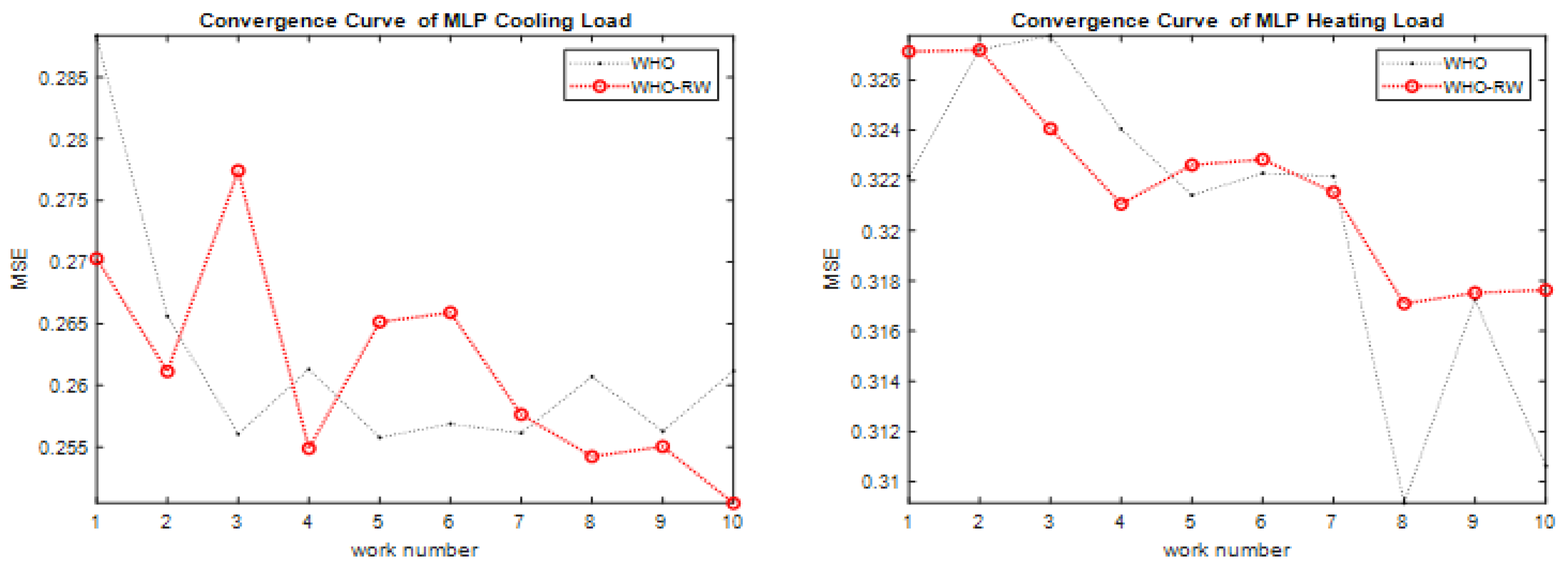
Efficient MLP training: the IWHO excels in training a Multi-Layer Perceptron for the energy efficiency problem, achieving lower MSE values and more reliable outcomes.

Improved prediction accuracy: the IWHO algorithm delivers higher prediction rates for Cooling Load (CL) factors than the original WHO algorithm.

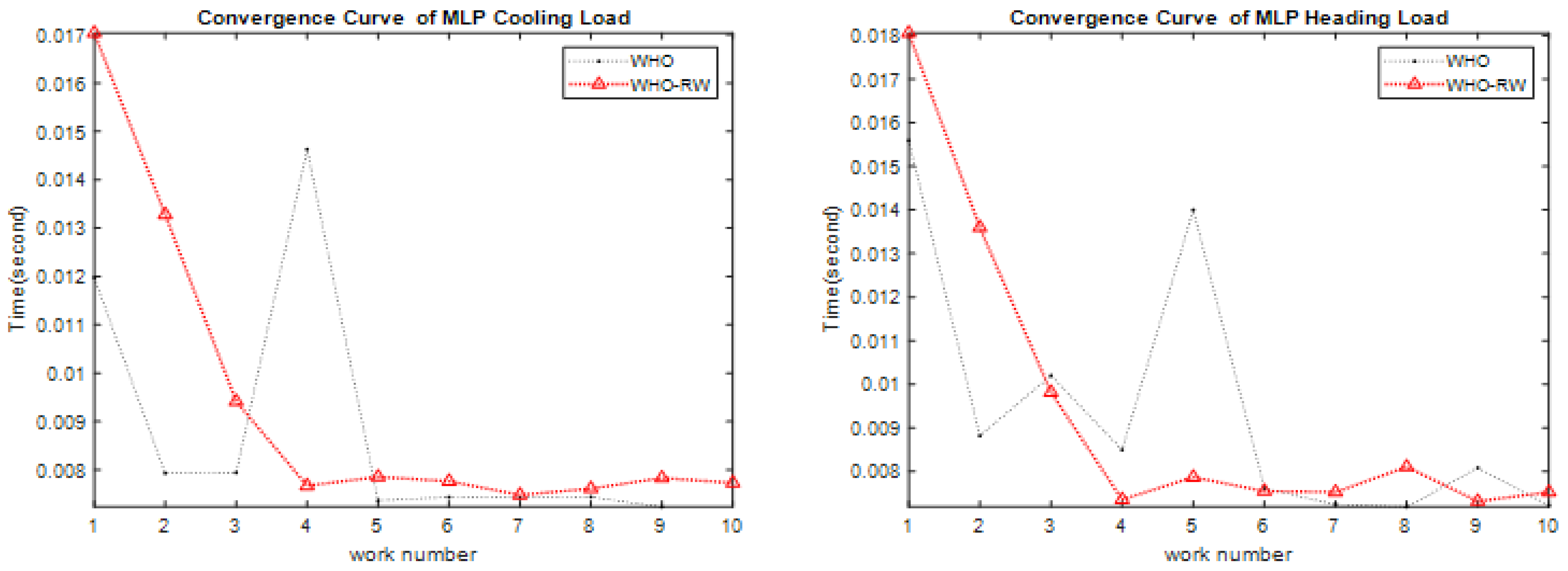
Time efficiency: despite its increased complexity, the IWHO completes the optimization process within a reasonable timeframe.

Flexibility and hybridization potential: the success of the IWHO suggests that the WHO algorithm possesses a flexible structure that is amenable to integration with other strategies.

Real-world applicability: the IWHO algorithm demonstrates potential for addressing practical issues such as optimizing HVAC systems in smart buildings for energy efficiency.

The remainder of the paper is organized as follows: Section 2 discusses the WHO algorithm, RW search strategy, and proposed IWHO hybridization structure. Section 3 presents the testing of the IWHO algorithm using the CEC 2019. Section 4 covers MLP training, and Section 5 presents the results.

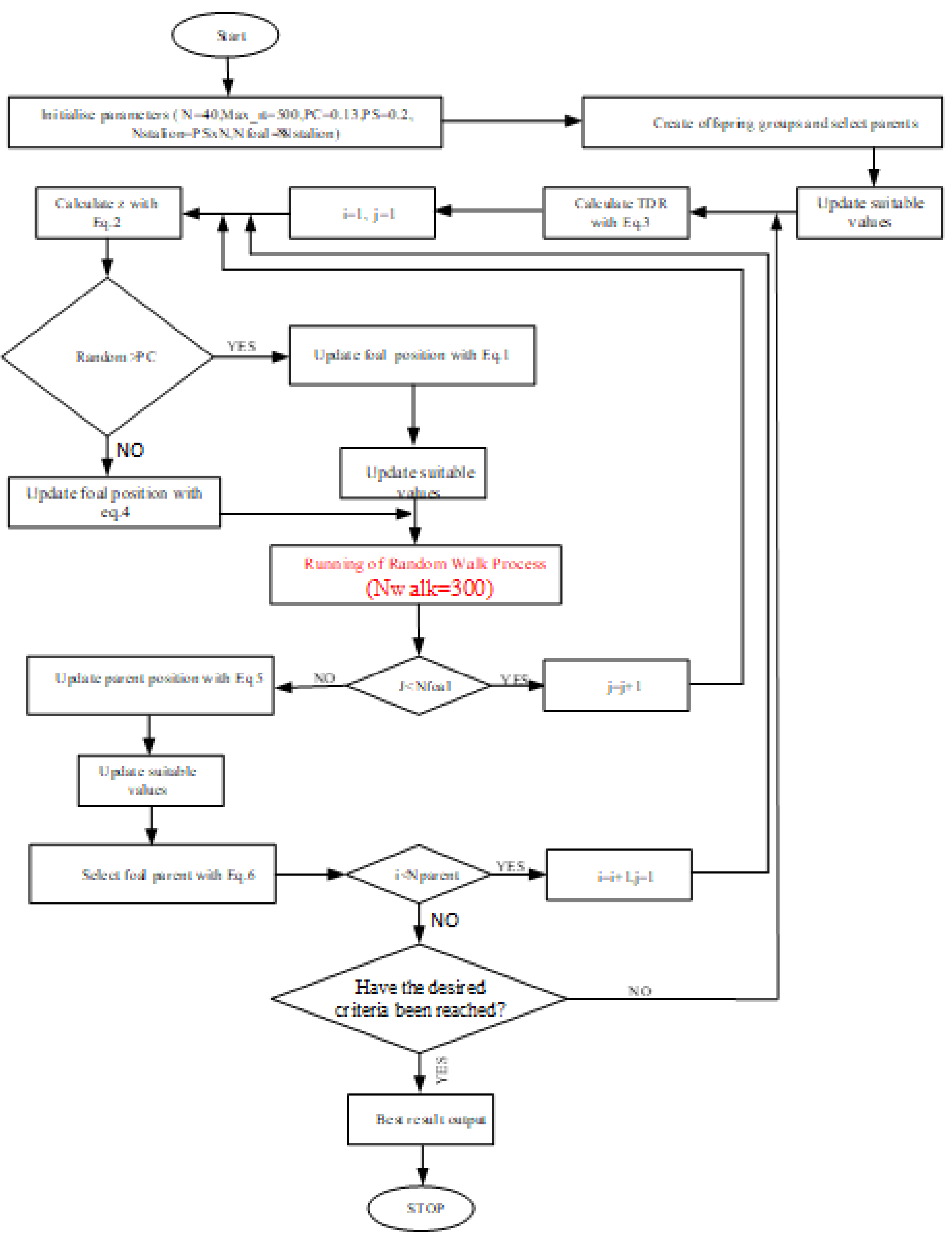
The proposed hybrid IWHO and the optimization process with alternative algorithms are given in Figure 1 below.

2. Algorithms

2.1. Wild Horse Optimizer (WHO)

The WHO algorithm is inspired by the common swarm behavior of wild animals. Figure 2 illustrates the swarm diagram of the WHO algorithm, which includes a swarm hierarchy (N), stallion (S), and foals (F), with each leader forming a group (G). As the foals mature, they leave the swarm to form their own independent families. The algorithm consists of five stages [32,46].

The algorithm starts the optimization process with a set of candidate solutions. In the initial set, the candidate horse simulation presents a certain hierarchy. In this hierarchy, there are groups of horses under different leaders. At this stage, a swarm diagram is generated as shown in Figure 2.

The ratio of the number of leaders $\left(PS\right)$ in a group,

$$PS={\displaystyle \frac{G_i}{N_i}},i=1,2,3,\dots$$

(1)

is determined by Equation (1).

In the second phase, the behavior of the swarm in the grazing pasture is modeled. The stallion (S) plays a central role in this behavior.

$$X_{G, j}^i=2Zcos\left(2\pi RZ\right)·\left({Stallion}_{G,j}-X_{G, j}^i\right)+{Stallion}_{G,j}$$

(2)

where j is the position of the members and stallions of group $i$ within the group is expressed by ${Stallion}_{G,j}$ and $X_{G, j}^i$. The parameter R is a random value in the open interval (−2, 2) and the parameter z is a self-adaptive parameter according to the changes in the process calculated in Equation (4) below.

$$P=\overrightarrow{r_1}<TDR, TDR=1-{\displaystyle \frac{it}{\mathrm{m}\mathrm{a}\mathrm{x}\_it}} IDX=\left(P==0\right)$$

(3)

$$z=r_2\theta IDX+\overrightarrow{r_3}\theta \left(~IDX\right)$$

(4)

where P and $r_1,r_2 \mathrm{v}\mathrm{e}{r}_3$ parameters are vectors that take random values in the range (0, 1). The current number of iterations is expressed as $it$, and the maximum number of iterations is expressed as $max\_it$.

Here, P is a vector containing 0 and 1 of a size equal to the size of the equation, and $r_1,r_2 \mathrm{a}\mathrm{n}\mathrm{d} r_3$ are vectors taking random values in the interval (0, 1). The current number of iterations is denoted by $it$ and the maximum number of iterations is denoted by $max\_it$.

In the third stage, Equation (1) simulates the mating behavior of horses. The swarm separates foals that have not yet reached mating age and prevents mating between parents and foals.

$$\begin{gathered} X_{G, k}^p=Crossover\left(X_{G,j}^q,X_{G, j}^z\right), i\ne j\ne k, q=z=end, \\ Crossover=mean \end{gathered}$$

(5)

In Equation (5), $X_{G, k}^p$ is the position of horse $p$ at position $k$, which includes the positions of horse $q$ in group i and horse z in group $j$. Here the crossover parameter Crossover percentage (PC) is adjustable.

In the fourth phase, the competition between group leaders is simulated with Equation (6). While the group leaders direct the other group members to the area with a suitable puddle, the winning group will have priority in the competition.

$${\overline{Stallion}}_{G,j}=\left\{\begin{array}{c}2Zcos\left(2\pi RZ\right)\times WH-\left({Stallion}_{G,j}\right)+WH, r_3>0.5\\ 2Zcos\left(2\pi RZ\right)\times WH-\left({Stallion}_{G,j}\right)-WH, r_3\le 0.5\end{array}\right.$$

(6)

where $WH$ is the location of the puddle, ${\overline{Stallion}}_{G,j}$ and ${Stallion}_{G,j}$ are the candidate position and current position of the leader, respectively.

In the final phase, leader selection is considered and simulated using Equation (7). Initially, the leader is randomly selected from the entire swarm, and then the stallion with the most favorable value becomes the leader.

$${Stallion}_{G,j}=\left\{\begin{array}{c}{X}_{G,j}^i\\ {Stallion}_{G,i}\end{array}\right.\begin{array}{c},f\left(X_{G,j}^i\right)<f\left({Stallion}_{G,j}\right)\\ ,f\left(X_{G,j}^i\right) \ge f\left({Stallion}_{G,j}\right)\end{array}$$

(7)

where $f\left(X_{G,j}^i\right)$ is the fitted value of foal, $f\left({Stallion}_{G,j}\right)$ is the fitted value of parents.

2.2. Random Walking Strategy

Metaheuristic algorithms employ randomization to identify optimal solutions, working with a set of candidate solutions to explore all possible paths for the best outcome. Achieving a global search requires reaching a local optimum, a process facilitated by non-deterministic randomization, which is also applied in local searches. Balancing local and global searches is crucial for evaluating the performance of metaheuristic algorithms [47]. The Random Walk strategy enhances this balance by introducing a predetermined number of random steps within defined boundaries. This strategy acts as a fine-tuning mechanism in later iterations, preventing the algorithm from becoming trapped in local optima [38,39,40]. The random walks method introduces diversity by disrupting the regular progression, interfering with future iterations to avoid premature entrapment in local optima. This approach aids in escaping local optima without reaching them too swiftly. During the exploration phase, as deviation decreases in subsequent iterations, progress is made, leading to less pronounced deviations and achieving stable outcomes. The parameter Walk, which determines the step size, allows random walks to be integrated into various search algorithms. It serves to perturb the population of solutions, thereby preventing entrapment in local optima. Selecting the step size distribution is vital in the search process. A small step size encourages the exploitation of the search space near the current state, focusing on refining existing solutions. Conversely, a sufficiently large step size promotes the exploration of uncharted areas within the search space, potentially uncovering new and promising regions for further investigation [47].

In this paper, by increasing the number of random steps through RW, the possibility of avoiding premature convergence and getting stuck at the local optimum is enhanced by delaying the discovery of the optimum point in the local search phase. In this strategy, the fitness values are differentiated by adjusting the position of the group leader according to a varying parameter.

$$\left.{\displaystyle \genfrac{}{}{0pt}{}{\mathrm{g}\mathrm{B}\mathrm{e}\mathrm{s}\mathrm{t}=\mathrm{W}\mathrm{H}.\mathrm{p}\mathrm{o}\mathrm{s}}{x_0=\mathrm{g}\mathrm{B}\mathrm{e}\mathrm{s}\mathrm{t}}}\right\}$$

(8)

$$x=x_0+Walk\times \left(0.5-rand(1\right))$$

(9)

where gBest is the best location of the puddle in Equation (8), $x$ represents the deviated value, $x_0$ is the current best position of the leader, and $Walk$ is the number of randomized steps in Equation (9). The flowchart of the IWHO algorithm is shown in Figure 3 and pseudo code is shown in Algorithm 1.

Algorithm 1: Pseudo Code of IWHO

1: Initialization

2: Set parameters:

3: $N=$ number of search agents (horses)

4: $t\_max=$ maximum number of iterations

5: $dim=$ problem dimension

6: $lb, ub=$ lower and upper bounds

7: $r=$ number of random walk steps

8: Generating Initial Population

9: for $i=1$ to N do

10:   $X\_i=$ random position within $[lb, ub]$

11:   Evaluate fitness $(X\_i)$

12: end for

13: Establish Hierarchy and Group Structure

14: Calculate $PS=$ ratio of leaders using Equation (1)

15: Divide population into groups with leaders

16: Main Loop

17: for $t=1$ to $t\_max$ do

18:    Update z parameter (self-adaptive)

19:    $z=2 \ast (1-{(t/t\_max)}^2)$

20:    Phase 1: Grazing behavior

21:    for each group $i$ do

22:      for each member $j$ in group $i$ do

23:         Update position using Equation (2)

24:         $R=$ random value in (−2, 2)

25:         $X\_ij=X\_ij+R \ast z \ast (X\_stallion-X\_ij)$

26:         Evaluate fitness $(X\_ij)$

27:      end for

28: end for

29:   Phase 2: Mating Behavior

30:   for each group $i$ do

31:      for each member j in group i do

32:         if random() < PC then // PC is crossover percentage

33:           Apply crossover using Equation (5)

34:           Select random horse z from different group k

35:           $X\_ij=crossover(X\_ij, X\_zk)$

36:           Evaluate fitness $(X\_ij)$

37:        end if

38:     end for

39: end for

40:   Phase 3: Competition Among Leaders

41:   for each leader $i$ do

42:       Update leader position using Equation (8)

43:       $X\_candidate=X\_i+random\left(\right) \ast (X\_puddle-X\_i)$

44:       if fitness $(X\_candidate)$ etter than fitness $(X\_i)$ then

45:            $X\_i=X\_candidate$

46:       end if

47: end for

48:    Phase 4: Leader Selection

49:    for each group $i$ do

50:       Select new leader using Equation (7)

51:       if any foal has better fitness than current leader then

52:             Update leader

53:       end if

54:    end for

55:    IMPROVEMENT: Random Walk Strategy

56:    for each leader $i$ do

57:      $best\_position=X_i$

58:      Execute Random Walk Steps

59:      for $step=1$ to r do

60:           Apply random walk using Equation (9)

61:           $X\_deviated=best\_position+random\_deviation\left(\right)$

62:           Ensure bounds

63:           $X\_deviated=max(lb, min(ub, X\_deviated\left)\right)$

64:           Evaluating New Position

65:           if fitness $(X\_deviated)$ better than fitness (best_position) then

66:             $best\_position=X\_deviated$

67:           end if

68:      end for

69:      Updating Leader with Best Position Found During Random Walk

70:      $X\_i=best\_position$

71:   end for

72:   Update Global Best Solution

73:   Update $X\_best$ if better solution found

74: end for

75: return $X\_best$

In accordance with the standard WHO phases, leaders engage in stochastic explorations, taking multiple steps to investigate the surrounding environment. This methodology assists in circumventing local optima and preventing premature convergence. The optimal position identified during these stochastic explorations is subsequently adopted. The random walk strategy constitutes a significant enhancement in IWHO compared to the original WHO algorithm, improving the exploration of the search space and facilitating the avoidance of local optima.

3. Multilayer Perceptron Architecture

The Multi-Layer Perceptron (MLP) is an artificial neural network architecture that serves as a nonparametric estimator, applicable for both classification, prediction, and regression tasks. The brain is an information processing device with extraordinary capabilities, surpassing current technological products in various fields such as vision, speech recognition, and learning. These applications have clear economic advantages when implemented on machines. By understanding how the brain accomplishes these functions, we can develop formal algorithms to solve these tasks and implement them on computers. The human brain is fundamentally different from a computer. While a computer typically has a single processor, the brain consists of an enormous number of processing units, approximately ${10}^{11}$ neurons, which operate in parallel. Although the precise details are not fully understood, these processing units are thought to be much simpler and slower than a computer processor. Another distinguishing feature of the brain, which is believed to contribute to its computational power, is its extensive connectivity. Neurons in the brain have connections, called synapses, to around ${10}^4$ other neurons, also functioning in parallel. In a computer, the processor is active and the memory is separate and passive; however, in the brain, it is believed that processing and memory are distributed throughout the network. Processing is carried out by the neurons, while memory resides in the synapses between neurons. The information processing system in the brain requires a fundamental theory, algorithm, and hardware. This includes data input for the desired operation, an algorithm to perform the function, and the capability to execute commands using a specific hardware implementation. The training of neural networks, which involves a mathematical function, is made possible through statistical techniques. One of the architectures designed for this training is the MLP structure [48].

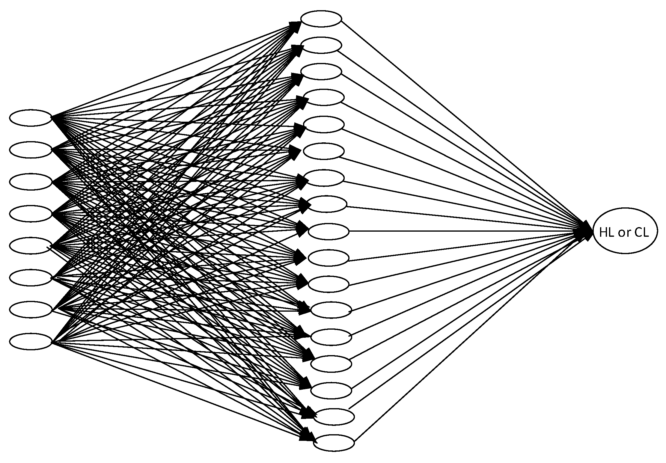
The aim of perceptron is to correctly classify the set of externally applied stimuli $x_1,x_2,\dots x_m$ into one of two classes. In Figure 4 bias denoted by b, $x_1,x_2,\dots x_m$ inputs value, $w_1,w_2,\dots w_m$ connection or synaptic weight, v induced local field of the neuron, and $\phi \left(v\right)$ transfer function. Given $v$ can also be defined as a hyperplane.

$$v=\sum _{i=1}^m{w}_i{x}_i+b$$

(10)

We can express the output of the perceptron as a dot product, and augmenting the input vector

$x={\left(x_1,x_2,\dots x_m\right)}^T$ and weight vector $w={\left(w_1,w_2,\dots w_m\right)}^T$ to include the bias weight and input, respectively.

$$v=w^{T}x$$

(11)

During testing, the output y is calculated with the given weights w for input x. To implement a given task, it is necessary to learn the weights w, which are the parameters of the system, such that the correct outputs are produced given the inputs.

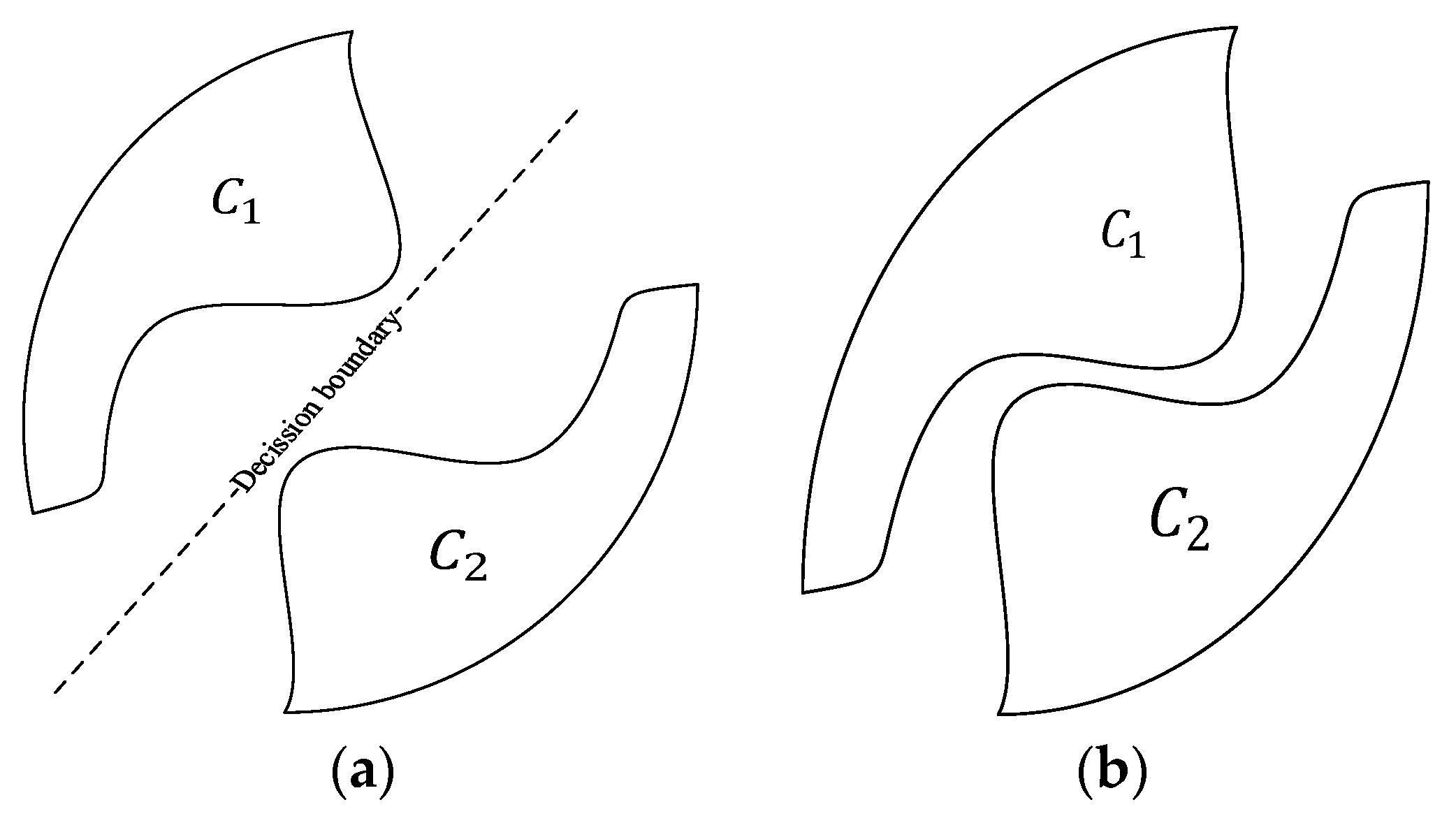
The hyperplane can be utilized to partition the input space into two regions: one where the values are positive and another where the values are negative. This concept is foundational in implementing a linear separation function. In Figure 5, the detector can then classify the input into one of two classes by examining the sign of the output: if the output is positive, it belongs to one class $\left(C_1\right)$; if negative, it belongs to the other class $\left(C_2\right)$ [49].

$$S\left(v\right)=\left\{\begin{array}{c}{ C}_1, S\left(v\right)>0\\ C_2, S\left(v\right)<0\end{array}\right.$$

(12)

If $x_i$ belongs to $C_1$ else $C_2$, $S\left(v\right)$ as a treshold function, We need to activation functon or output (y) for calculate risk. The transfer function is the mathematical function that defines the properties of the network and is chosen according to the problem that the network has to solve. The reason for choosing sigmoid as the transfer function in this paper is that it has continuous and differentiable values in the interval [0, 1]. Here the parameter a is the slope of the transfer function.

$$y=sigmoid\left(v\right)={\displaystyle \frac{1}{1+e^{\left(-av\right)}}}$$

(13)

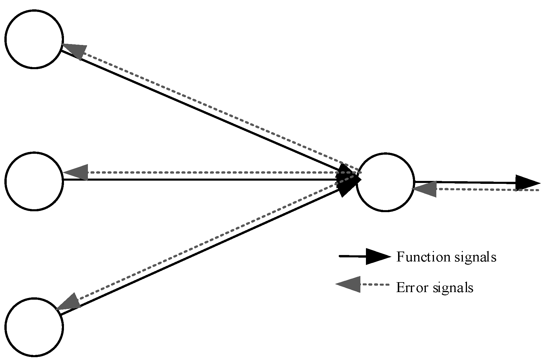
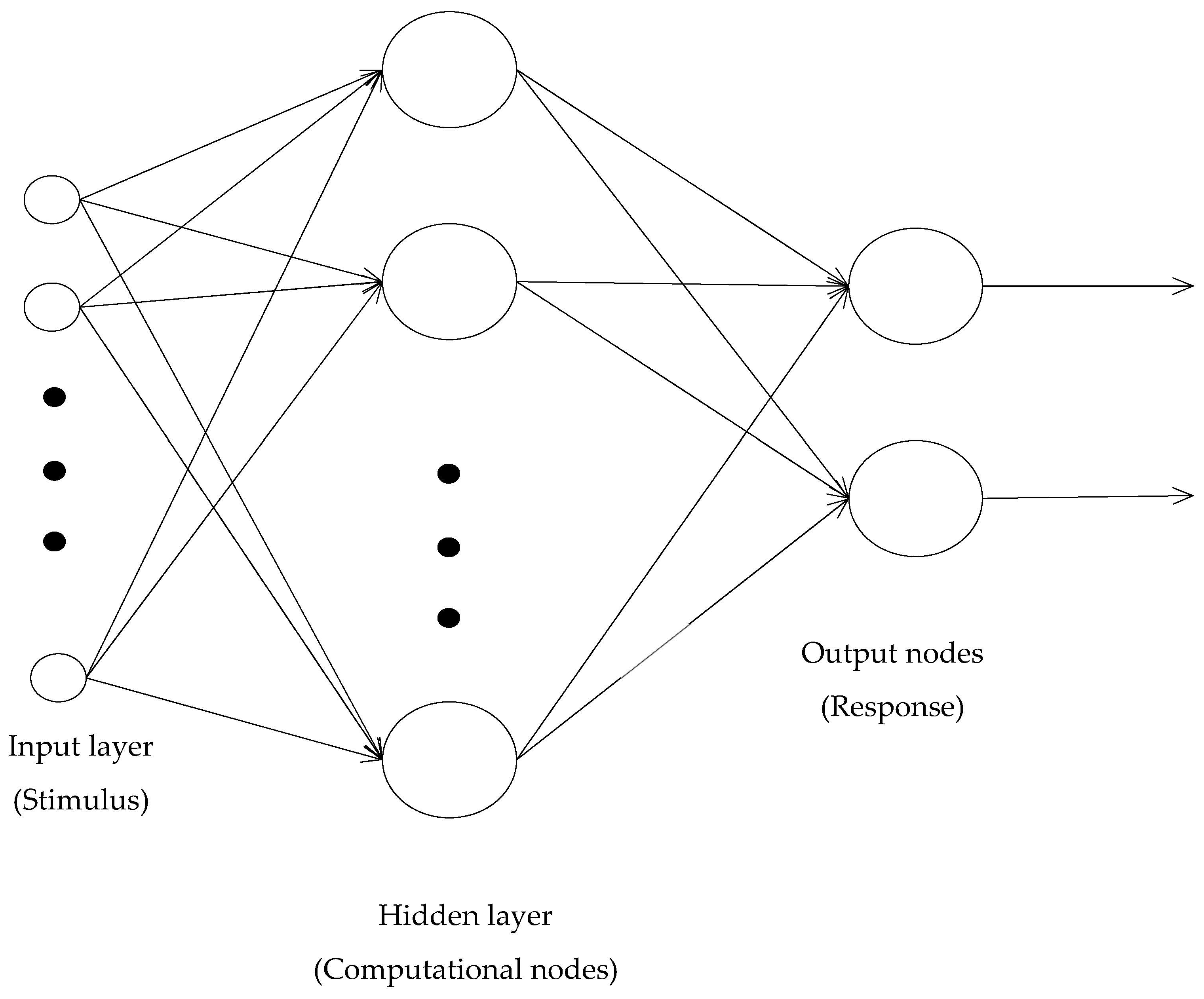
A perceptron with a single layer of weights can only approximate linear functions of the input and cannot solve problems like XOR, where the discriminant to be estimated is nonlinear. Similarly, a perceptron cannot be used for nonlinear regression. This limitation does not apply to feedforward networks with hidden layers between the input and output layers. When used for classification, such Multi-Layer Perceptrons can implement nonlinear discriminants, and when used for regression, they can approximate nonlinear functions of the input. Typically, the network consists of a set of source nodes that constitute the input layer, one or more hidden layers of computation nodes, and an output layer of computation nodes. These neural networks are called Multi-Layer Perceptrons (MLPs), representing a generalization of the single-layer perceptron. MLPs have been applied successfully to solve some difficult and diverse problems by training them in a supervised manner with a viral algorithm known as “backprop”. The learning process performed with this algorithm is called backpropagation learning. As seen Figure 6 in an MLP, while function signals flow in the forward propagation direction, the error signal responds with the backpropagation flow and is corrected to minimize the error. An error signal begins at an output neuron of the network and travels backward through the network. Each neuron in the network computes using a function namely error that depends on the error in some way [49,50].

Learning is a process in which the free parameters of a neural network are adapted by the environment in which the network is embedded through a simulation process shown as Figure 7. The type of learning is determined by the way parameter changes take place [50].

Error metrics serve as a quantitative measure of the deviation between predicted outcomes and actual values. While a single result may not yield extensive insights, it facilitates the selection of the most appropriate regression model by providing a numerical basis for comparison with other model outcomes. The supervisor can provide the neural network with the desired response for a specific training vector, representing the optimal action the network should undertake. The network parameters are adjusted under the combined influence of the training vector and the error signal, defined as the difference between the desired and actual responses of the network. This tuning process is conducted iteratively and incrementally, with the objective of ensuring that the neural network eventually emulates the supervisor, which is presumed to be optimal in a statistical sense. Through this process, the environmental information available to the supervisor is transferred as comprehensively as possible to the neural network during training. Once this condition is achieved, the tutor can be dispensed with, allowing the neural network to independently interact with the environment. Error values can be calculated using metrics such as mean squared error (MSE), root mean square error (RMSE), mean absolute error (MAE), mean absolute percentage error (MAPE), and the coefficient of determination ($R^2$).

$$MSE={\displaystyle \frac{1}{N}}\sum _{i=1}^N{\left(P_i-O_i\right)}^2$$

(14)

$$RMSE=\sqrt{MSE}$$

(15)

$$MAE={\displaystyle \frac{1}{N}}\sum _{i=1}^N\left|P_i-O_i\right|$$

(16)

$$MAPE={\displaystyle \frac{MAE}{AVERAGE TRUE VALUE}}\ast 100$$

(17)

$$R^2=1-{\displaystyle \frac{{\sum }_{i=1}^N{\left(P_i-O_i\right)}^2}{{\sum }_{i=1}^N{\left(P_i-\overline{P_i}\right)}^2}}$$

(18)

In Equation (14) $N$ is the training samples, $i$ is the number of outputs value, $P_i$ is the desired output, and $O_i$ actual output.

4. Experimental Results

The main goal of this paper is to solve a global non-parametric standardized function set using the WHO algorithm (IWHO) hybridized with the Random Walk strategy and to compare the results with those of alternative competitive metaheuristic algorithms. A notation table summarizing all parameters of the algorithm has been added as

Table 1. Algorithm parameters.

Parameter	Statement	Value
$N$	Number of search agents	40
$t_{max}$	Maximum number of iterations	500
$d$	Problem dimension	9, 10, 16, 18 (see CEC 2019 functions)
lb, ub	Lower and upper bounds	[−100, 100]
r	Number of random walk steps	300
$x_i$	Position of the i-th horse/agent	-
$x_{i,j}$	Position of the j-th member in group i	-
$x_{stallion}$	Position of the group leader (stallion)	-
z	Self-adaptive parameter	z = 2 × (1 − (t/t_max)2)
$R$	Random value in update equations	R ∈ (−2, 2)
$P$	Random vector	P ∈ (0, 1)
$PC$	Crossover percentage	Adjustable
Hardware	CPU used for experiments	Intel Core i7-10700K, 32 GB RAM
Software	MATLAB version	R2021a (parallel processing enabled)

.

The analysis tools used include statistical tables, boxplots, and convergence curve. The CEC 2019 functions are among the most challenging non-linear function sets due to their structure, which delays reaching the global solution, and are widely accepted for evaluating algorithm quality. The primary rationale for selecting only 10 functions from the CEC 2019 set in our research is that these functions are internationally recognized as a challenging and diverse benchmark. The CEC 2019 functions are designed to evaluate the effectiveness of optimization algorithms, encompassing a wide range of problem types and complexities. This variety is sufficient for an objective assessment of both the algorithms’ convergence speed and their ability to identify the global optimum. As indicated in the manuscript (refer to

Table 2. Set of CEC 2019 benchmark functions.

Functions	Dimension	Bounds	Fitting Value
CEC01: Storn’s Chebyshev Polynomial Fitting Problem	9	[−8192, 8192]	1
CEC02: Inverse Hilbert Matrix Problem	16	[−16,384, 16,384]	1
CEC03: Lennard–Jones Minimum Energy Cluster	18	[−4, 4]	1
CEC04: Rastrigin’s Function	10	[−100, 100]	1
CEC05: Griewangk’s Function	10	[−100, 100]	1
CEC06: Weierstrass Function	10	[−100, 100]	1
CEC07: Modified Schwefel’s Function	10	[−100, 100]	1
CEC08: Expanded Schafer’s F6 Function	10	[−100, 100]	1
CEC09: Happy Cat Function	10	[−100, 100]	1
CEC10: Ackley Function	10	[−100, 100]	1

), the selected 10 functions vary in dimension, range, and problem type, providing adequate challenge and diversity to thoroughly evaluate the algorithms’ performance. These functions constitute the core and most frequently cited subset of the CEC 2019 benchmark. The specified the hardware used (Intel Core i7-10700K CPU, 32 GB RAM) and MATLAB settings (R2021a, parallel processing enabled). For IWHO, 40 search agents, 500 iterations, and 300 Random Walk steps were chosen. Each function was tested in 51 independent runs, a number that ensures the results are more objective and reliable.

In Table 2, CEC 2019 featured demonstration. In

Table 3. Performance results of functions.

	Score
Func.	Metric	WHO	IWHO	CapSA	HHO
CEC01	Mean	5.34 × 104	4.21 × 104	5.01 × 104	5.11 × 104
	Std	4.62 × 104	4.17 × 104	5.39 × 104	6.15 × 103
	Best	3.54 × 104	3.15 × 104	3.59 × 104	4.28 × 104
	Worst	3.60 × 105	3.34 × 105	3.18 × 105	7.30 × 104
CEC02	Mean	17.3	17.3	17.3	17.4
	Std	2.15 × 10−14	2.15 × 10−14	8.80 × 10−5	9.99 × 10−3
	Best	17.3	17.3	17.3	17.3
	Worst	17.3	17.3	17.3	17.4
CEC03	Mean	12.7	12.7	12.7	12.7
	Std	3.15 × 10−6	2.36 × 10−7	2.21 × 10−17	6.49 × 10−6
	Best	12.7	12.7	12.7	12.7
	Worst	12.7	12.7	12.7	12.7
CEC04	Mean	26.2	28.7	41.2	180
	Std	15.7	23.6	21	62.9
	Best	5.97	8.95	8.96	86
	Worst	86.6	124	105	380
CEC05	Mean	1.07	1.05	1.19	2.45
	Std	0.071	0.029	0.108	0.515
	Best	1.01	1.00	1.02	1.27
	Worst	1.49	1.14	1.59	3.86
CEC06	Mean	5.60	3.60	7.64	9.03
	Std	0.928	0.987	1.23	1.11
	Best	3.53	1.53	4.66	5.75
	Worst	7.37	6.02	10.3	11.1
CEC07	Mean	122	60.1	463	361
	Std	125	126	307	178
	Best	−205	-253	−166	182
	Worst	369	273	1000	939
CEC08	Mean	4.74	4.33	5.39	5.77
	Std	0.643	0.706	84.9	0.484
	Best	3.33	2.90	3.06	4.59
	Worst	5.88	5.70	6.84	6.76
CEC09	Mean	2.45	2.38	2.53	3.15
	Std	0.129	0.0319	0.160	0.449
	Best	2.35	2.34	2.35	2.48
	Worst	3.10	2.48	2.98	4.64
CEC10	Mean	20	19.6	20.1	20.2
	Std	0.0091	2.64	0.0995	0.0952
	Best	20	1.16	20	20
	Worst	20	20	20.4	20.4

, mean, best value, worst value, and standard deviation are used as statistical measures to evaluate the suitability of the values obtained by the algorithms.

When examining Table 3, the proposed IWHO algorithm achieves the best value in all functions except CEC03 and CEC04. For CEC03, all algorithms yield the same results with different standard deviations. In this case, WHO performs very well, and the proposed IWHO algorithm ranks second.

The IWHO algorithm proposed in this paper is compared with the WHOFWA and WHOW algorithms, which were previously proposed as variants of WHO. It is also compared with the RW-DO algorithm, which has been studied with the random walking strategy in the IWHO algorithm. As a result, as shown in

Table 4. Comparison of IWHO with other hybrid algorithms.

Func.	Metric		Score
-	-	IWHO	WHOFWA [51]	WHOW [35]	RW-DO [45]
CEC01	Mean	4.21 × 1004	4.76 × 104	7.59 × 104	1.01 × 1012
	Std	4.17 × 104	47.1	4.57 × 104	5.48 × 1012
CEC02	Mean	17.3	17.3	17.3	754
	Std	2.15 × 10−14	2.09 × 10−5	8.31 × 10−14	4.03 × 103
CEC03	Mean	12.7	12.7	12.7	12.7
	Std	2.36 × 10−7	8.75 × 10−10	3.95 × 10−15	3.24 × 10−4
CEC04	Mean	28.7	46.2	22.9	2.00 × 103
	Std	23.6	16.8	5.03	5.18 × 104
CEC05	Mean	1.05	1.31	1.08	2.22
	Std	0.0286	0.141	0.0393	1.12
CEC06	Mean	3.60	4.73	5.78	1.55
	Std	0.987	0.960	0.606	6.87
CEC07	Mean	60.1	-	154	585
	Std	126	-	56	381
CEC08	Mean	4.33	5.10	4.88	6.03
	Std	0.706	6.57	0.511	0.888
CEC09	Mean	2.38	2.57	2.67	258
	Std	0.0319	0.126	0.129	1.22 × 103
CEC10	Mean	19.6	19.4	20	20.5
	Std	2.64	3.23	9.41 × 10−3	0.217

the IWHO algorithm has a superior performance in seven functions.

In

Table 5. Wilcoxon test results.

Functions	Metrics	WHO	CapSA	HHO
CEC01	p-value	3.03 × 10−4	2.80 × 10−3	9.66 × 10−5
	W/T/L	W	W	W
CEC02	p-value	1.00	5.15 × 10−10	5.15 × 10−10
	W/T/L	L	W	W
CEC03	p-value	1.00	0.5	5.15 × 10−10
	W/T/L	L	W	W
CEC04	p-value	0.7786	2.27 × 10−5	5.47 × 10−10
	W/T/L	L	W	W
CEC05	p-value	0.107	1.40 × 10−9	5.15 × 10−10
	W/T/L	T	W	W
CEC06	p-value	8.27 × 10−10	5.15 × 10−10	5.15 × 10−10
	W/T/L	W	W	W
CEC07	p-value	0.325	8.65 × 10−9	7.80 × 10−10
	W/T/L	L	W	W
CEC08	p-value	0.593	8.61 × 10−7	3.94 × 10−9
	W/T/L	L	W	W
CEC09	p-value	2.27 × 10−5	7.32 × 10−9	5.15 × 10−10
	W/T/L	W	W	W
CEC10	p-value	6.70 × 10−8	5.15 × 10−10	5.15 × 10−10
	W/T/L	W	W	W

, the nonparametric Wilcoxon test was used to evaluate whether the proposed IWHO algorithm differs from other algorithms when working with a different data set, assessing its originality. In this context, W (Win) represents a victory, T (Till) a draw, and L (Low) a defeat. The confidence level was set at p = 0.05. From the results, it can be concluded that the proposed IWHO algorithm is unique and original, as it produced significantly different results with 24 wins, 1 tills, and 5 losses out of 30 results.

Table 5 analyzed, The Wilcoxon signed-rank test was employed to assess if there was a statistically significant difference in the performance of the two algorithms. Table 5: W/T/L: These letters stand for ‘Win’, ‘Tie’, and ‘Lose’, respectively, reflecting the status of the IWHO algorithm in comparison to other algorithms. p-value: A value under 0.05 was deemed to indicate statistical significance. The IWHO algorithm demonstrated notable superiority (W) over the CAPSA and HHO algorithms for almost all functions. When compared to the WHO algorithm, it was superior in some functions and either matched or fell short in others. Remarkably, against CAPSA and HHO, the IWHO excelled in nine or all ten functions. The p-values were mostly very small (e.g., 5.15 × 10⁻¹⁰), indicating that the observed difference is unlikely to be by chance, but rather that the IWHO’s superiority is statistically sound. The results of the Wilcoxon signed-rank test reveal that the IWHO algorithm is statistically significantly superior in nearly all CEC 2019 functions, especially when compared to the CAPSA and HHO algorithms. Although it surpassed the WHO algorithm in certain functions, it showed similar or lower performance in others. These findings imply that the IWHO is generally a more effective and dependable optimization algorithm than its competitors.

Benferroni correction was used. Taking into account the ${(p}_{values}<0.05/30)$ evaluation, all elements of the h vector were 1. This result shows that the functions are significant according to the Benferroni test.

This paper performs a sensitivity analysis to determine the optimal beta parameter values within the RW-DO algorithm. For this purpose, the CEC 2019 benchmark, consisting of ten distinct functions, was chosen. The parameter C was tested at values of 0.12, 0.13, and 0.14, while the parameter ps remained constant at 0.2. The effects of these adjustments on the IWHO algorithm were evaluated. Although the results for CEC 06 did not produce the best standard deviation, the outcomes for all other functions were favorable. These results are detailed in the accompanying

Table 6. Sensitivity analysis for RW = 300.

	RW = 300 and Population Size = 40				RW = 300 and Population Size = 50
Function	Metric (ps = 0.2)	PC = 0.12	PC = 0.13	PC = 0.14	Metric (ps = 0.2)	PC = 0.12	PC = 0.13	PC = 0.14
CEC 2019
CEC01	Mean	6.89 × 108	6.41 × 108	7.67 × 108	Mean	5.74 × 108	4.52 × 108	4.66 × 108
	Std	1.04 × 109	6.82 × 108	1.16 × 109	Std	8.51 × 108	3.86 × 108	1.77 × 108
CEC02	Mean	1.73 × 105	1.73 × 105	1.73 × 105	Mean	1.73 × 105	1.73 × 105	1.73 × 105
	Std	0	0	1.40 × 10−10	Std	0	0	0
CEC03	Mean	1.27 × 105	1.27 × 105	1.27 × 105	Mean	1.27 × 105	1.27 × 105	1.27 × 105
	Std	1.40 × 10−2	2.18 × 10−10	0	Std	1.57 × 10−1	9.62 × 10−3	8.93 × 10−3
CEC04	Mean	3.25 × 105	2.46 × 105	3.62 × 105	Mean	1.98 × 105	1.71 × 105	1.76 × 105
	Std	5.34 × 105	1.21 × 105	6.28 × 105	Std	1.00 × 105	1.50 × 105	7.38 × 105
CEC05	Mean	1.06 × 104	1.05 × 104	1.06 × 104	Mean	1.04 × 104	1.03 × 105	1.05 × 104
	Std	431	292	475	Std	279	244	269
CEC06	Mean	5.40 × 104	5.54 × 104	5.40 × 104	Mean	5.22 × 104	5.15 × 104	5.24 × 104
	Std	1.07 × 104	8.05 × 103	8.27 × 103	Std	9.78 × 103	8.47 × 103	7.89 × 103
CEC07	Mean	1.28 × 106	1.27 × 106	1.29 × 106	Mean	7.41 × 105	7.32 × 105	1.20 × 106
	Std	1.37 × 106	1.30 × 106	1.35 × 106	Std	1.31 × 106	1.21 × 106	1.11 × 106
CEC08	Mean	4.78 × 104	4.50 × 104	4.69 × 104	Mean	4.64 × 104	4.35 × 104	4.49 × 104
	Std	7.51 × 103	6.54 × 103	6.96 × 103	Std	5.05 × 103	7.43 × 103	7.15 × 103
CEC09	Mean	2.44 × 104	2.43 × 104	2.44 × 104	Mean	2.39 × 104	2.30 × 104	2.39 × 104
	Std	661	913	675	Std	306	762	502
CEC10	Mean	1.97 × 105	1.96 × 105	2.00 × 105	Mean	2.00 × 105	1.90 × 105	2.00 × 105
	Std	2.52 × 104	82.2	2.64 × 104	Std	48.5	38.2	132

and

Table 7. Sensitivity analysis for RW = 500.

	RW = 500 and Population Size = 40				RW = 500 and Population Size = 50
Function	Metric (ps = 0.2)	PC = 0.12	PC = 0.13	PC = 0.14	Metric (ps = 0.2)	PC = 0.12	PC = 0.13	PC = 0.14
CEC 2019
CEC01	Mean	3.30 × 109	5.17 × 108	6.16 × 108	Mean	4.27 × 108	7.56 × 108	7.06 × 108
	Std	1.26 × 1010	2.20 × 108	6.61 × 108	Std	4.01 × 107	1.44 × 109	1.23 × 109
CEC02	Mean	1.73 × 105	1.73 × 105	1.73 × 105	Mean	1.73 × 105	1.73 × 105	1.73 × 105
	Std	0	0	0	Std	3.61 × 10−11	3.61 × 10−11	0
CEC03	Mean	1.27 × 105	1.27 × 105	1.27 × 105	Mean	1.27 × 105	1.27 × 105	1.27 × 105
	Std	5.48 × 10−11	5.48 × 10−11	3.86 × 10−3	Std	5.48 × 10−11	3.86 × 10−3	5.48 × 10−11
CEC04	Mean	5.18 × 105	2.25 × 105	2.32 × 105	Mean	2.45 × 105	2.31 × 105	2.38 × 105
	Std	8.78 × 105	1.61 × 105	1.19 × 105	Std	1.08 × 105	1.18 × 105	1.43 × 105
CEC05	Mean	1.05 × 104	1.06 × 104	1.06 × 104	Mean	1.05 × 104	1.04 × 104	1.04 × 104
	Std	3.86 × 102	3.80 × 102	3.39 × 102	Std	2.74 × 102	3.30 × 102	2.35 × 102
CEC06	Mean	5.58 × 104	5.14 × 104	5.32 × 104	Mean	5.57 × 104	5.09 × 104	5.20 × 104
	Std	1.13 × 104	1.34 × 104	9.04 × 103	Std	6.66 × 103	1.07 × 104	9.77 × 103
CEC07	Mean	1.29 × 106	9.15 × 105	9.26 × 105	Mean	9.52 × 105	7.05 × 105	7.18 × 105
	Std	9.83 × 105	1.29 × 106	1.16 × 106	Std	9.11 × 105	1.03 × 106	1.39 × 106
CEC08	Mean	4.60 × 104	4.48 × 104	4.81 × 104	Mean	4.76 × 104	4.36 × 104	4.43 × 104
	Std	5.21 × 103	8.35 × 103	5.35 × 103	Std	4.68 × 103	9.39 × 103	7.79 × 103
CEC09	Mean	2.47 × 104	2.43 × 104	2.46 × 104	Mean	2.40 × 104	2.37 × 104	2.39 × 104
	Std	1.91 × 103	7.42 × 102	1.09 × 103	Std	5.48 × 102	4.26 × 102	3.86 × 102
CEC10	Mean	1.91 × 105	2.00 × 105	1.81 × 105	Mean	2.00 × 105	1.80 × 105	1.89 × 105
	Std	4.06 × 104	1.06 × 102	5.67 × 104	Std	62.1	228	4.59 × 104

.

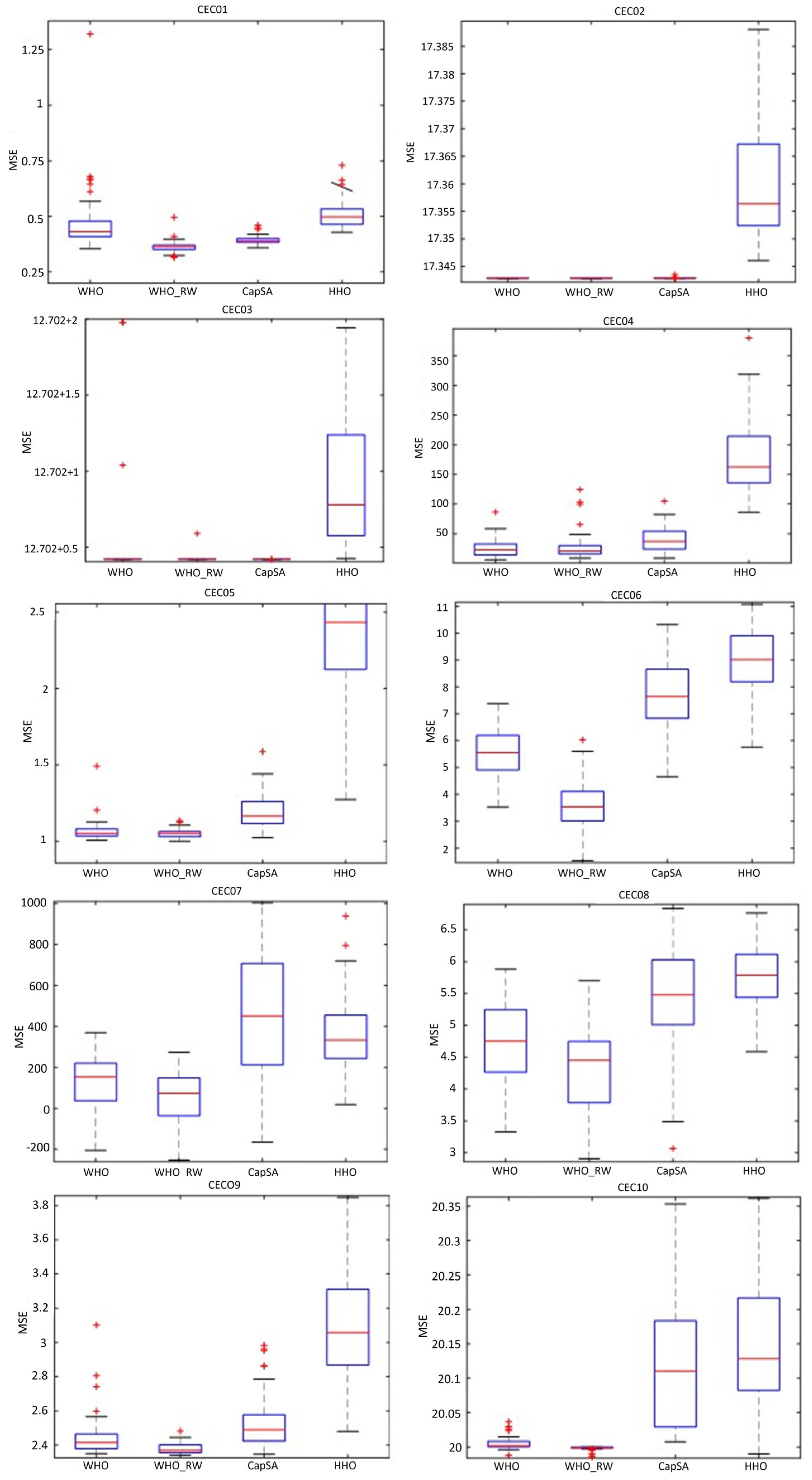
Upon reviewing Figure 8, it becomes evident that the values produced by the proposed IWHO algorithm are more closely clustered across all functions, making it the algorithm nearest to the optimal point compared to others. The whiskers and boxes for the CEC01 function in both the WHO and IWHO algorithms are notably lower and shorter than those of HHO and CapSA. This indicates that WHO and IWHO achieve superior (lower MSE) and more consistent results. The lowest whisker point suggests that these algorithms may be closer to, or have reached, the global optimum. For the CEC02 function, WHO, IWHO, and CapSA show very short whiskers and low boxes, while HHO is significantly higher and more variable. It is likely that WHO and IWHO have reached the global optimum. Similarly, for the CEC03 function, the whiskers for WHO and IWHO are the lowest, whereas HHO is considerably higher, further indicating that WHO and IWHO are closer to the global optimum. Across functions in the range CEC04-CEC10, WHO and IWHO display the lowest whisker values, suggesting that these algorithms yield superior results (closer to the global optimum) compared to the others. Although a few outlier values are observed in the CEC01, CEC03, CEC04, and CEC10 functions, the consistency of results from fifty-one independent runs highlights the algorithm’s stable structure. Consequently, it can be concluded that the global solutions of this algorithm are within the best limits and closer to the optimal global solution.

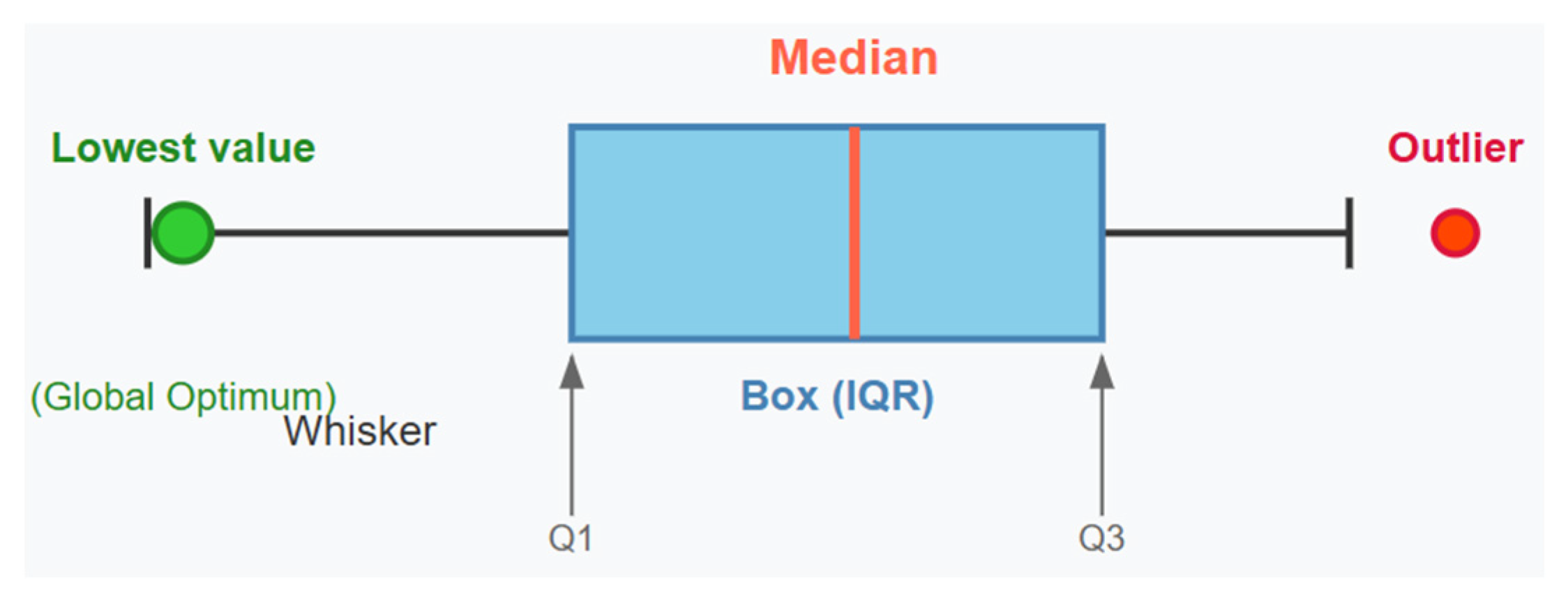
As seen in the box plot model in Figure 9, box plots are displayed as lines with whiskers extending from the box to the minimum and maximum non-outlier values, revealing the spread of the data. The lowest point reached by the whisker, or the lowest outlier, might represent the optimal value (global optimum) identified by the algorithm, assuming it aligns with the true global optimum of the function. In a boxplot, the whiskers extend from the box to the minimum and maximum non-outlier values, indicating the spread of most of the data. The box itself represents the interquartile range (IQR), which encompasses the middle 50% of the data, from the first quartile (Q1) to the third quartile (Q3). The thick line within the box signifies the median, or the 50th percentile, of the data. Any data point outside the whiskers is considered an outlier and is depicted as a red dot. The lowest value reached by the left whisker, or the lowest outlier, might represent the optimal value (global optimum) identified by an optimization algorithm, provided it corresponds to the true minimum of the function.

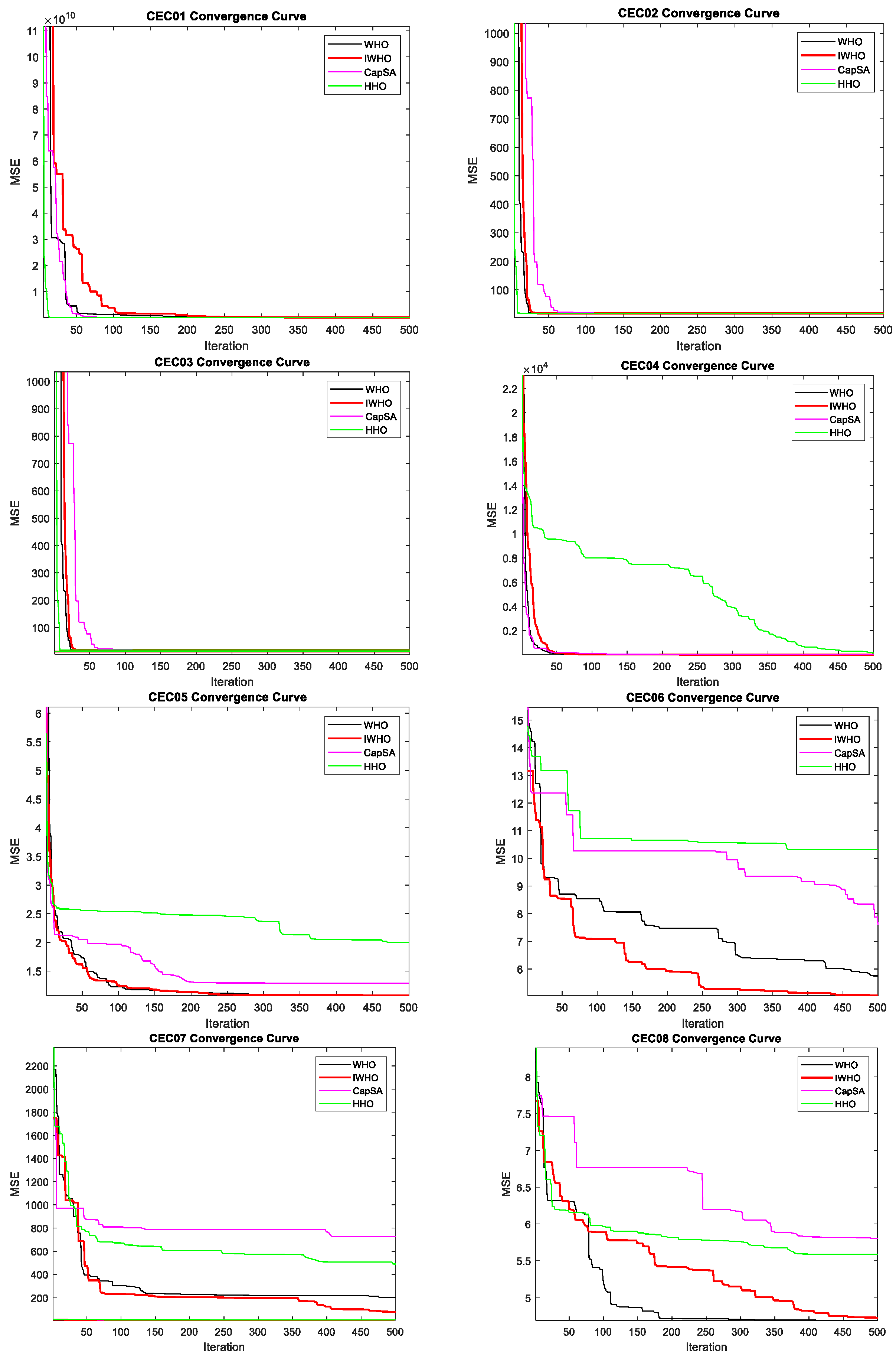
Convergence curves determine how the algorithms approach the optimal value over 500 iterations, whether they get stuck at local minimum points, and if they are subject to premature convergence. In this context, Figure 10 shows that the proposed IWHO algorithm progresses gradually in all functions without early convergence. Observing that the IWHO algorithm does not show constant progress in a certain range of iterations, but instead continually moves towards better solutions, can be considered proof that the IWHO algorithm reaches the global solution without getting stuck at local optima. As a result, it can be observed that the IWHO algorithm converges towards the optimal point across the entire function set.

5. MLP Training with the Proposed IWHO Algorithm

Solving Energy Efficiency Problem with IWHO-Based MLP Training

The main aim of this chapter is to optimize the efficiency of energy load factors in heating, ventilation, and air conditioning (HVAC) systems used in smart buildings. Energy used in buildings is consumed through (HVAC) systems. The HVAC system is designed to create suitable indoor air conditions by heating, cooling, and ventilating the air inside the building, and in this process, it calculates the building’s heat load (HL) and cooling load (CL) factors. Accurate estimation of HL and CL factors in buildings is important for reducing energy consumption based on occupancy, managing changes in building performance according to energy demands, reducing harmful gas emissions, and lowering costs. The necessary cooling and heating capacities are estimated based on fundamental factors such as building characteristics, usage, and climate conditions. The optimal design of the HVAC system plays a critical role in ensuring energy savings. In this context, the interior design of buildings is important not only for saving energy consumption but also for human health. To achieve energy savings, HVAC systems, which are generally preferred as active systems, are used. To maximize efficiency and energy savings, HVAC systems should be designed according to the building’s climate conditions [52,53,54,55].

The MLP (Multi-Layer Perceptron) architecture is designed according to the dimensions of the selected problem. In this article, the Energy Efficiency problem dataset has 8 features. Therefore, the input signal of the network consists of eight features. These features are: Relative Compactness, Surface Area, Wall Area, Roof Area, Overall Height, Orientation, Glazing Area, and Glazing Area Distribution. The output signals are defined as Heating Load and Cooling Load. The number of nodes in the hidden layer, which is located between the input and output layers, is 17, which is one more than twice the 8 nodes in the input layer. This choice is an arbitrary selection found to be appropriate by the author.

In Figure 11, the simulation of the MLP architecture created for the Energy Efficiency Problem dataset is drawn.

In the architecture shown in Figure 11, MSE is assigned as the error rate, and the sigmoid function is assigned as the transfer function. While cooling load specifies a different working universe, heating load specifies a different working universe, so a single output is used. Both WHO and the proposed IWHO hybrid algorithms were selected as advisors, and MLP training was performed. The results of the MLP training were statistically evaluated. While the running time of WHO is 0.0087 on average for 10 independent runs, the running time of IWHO is 0.0107. Although the parameters added for the hybrid algorithm result in an average delay of 22.98% in time, the optimization processes of the algorithms are fast given the short time spent on each iteration. The comparative results of WHO and IWHO for cooling load and heating load are shown in

Table 8. Results of regression measures.

Metric	WHO		IWHO
W	Cooling Load	Heating Load	Cooling Load	Heating Load
MSE	2.65 × 10−1	0.333	0.257	0.314
RMSE	0.515	0.568	0.508	0.561
MAE	0.42	0.47	0.43	0.48
MAPE	1.7%	1.9%	1.7%	1.9%
R2	0.981	0.980	0.985	0.983

.

The IWHO algorithm exhibits strong regression performance, evidenced by low error metrics (MSE, RMSE, MAE) and significant explanatory power (R²) for both Cooling and Heating Load. MAPE values under 2% indicate that the model’s predictions are closely aligned with the actual values. An R² value above 0.98 suggests that the model accounts for nearly all the variance in the data.

As a second analysis, when examining the convergence curves of WHO and IWHO values for average MSE, as shown in Figure 12, the MSE values of the IWHO algorithm for CL were lower than those of WHO in 6 runs and were also more consistent. Similarly, for HL the MSE values of the IWHO algorithm were closer together and more stable compared to the WHO algorithm. The comparative convergence curve of WHO and WHO-RW for cooling load and heating load are shown in Figure 13.

As a third analysis, when the WHO and IWHO algorithms are compared in terms of prediction rates, the average prediction value of the WHO algorithm for the CL factor is 99.6980 ± 1.4980 × 10⁻¹⁴; for IWHO, this value is 99.7010 ± 1.1751 × 10⁻¹⁴. For the HL factor, the average prediction value of the WHO algorithm is 100; for IWHO, this value is also 100.

As a fourth analysis, it is recommended to include a concise discussion on computational complexity, specifically using Big-O notation, along with a plot illustrating runtime against population size or iterations. It is essential to specify the hardware utilized (CPU/GPU) and any MATLAB configurations employed. The computational complexity of the IWHO algorithm introduced in this study is influenced by several parameters: the swarm size (N), the maximum number of iterations (t), the number of random walk steps (s), and the problem size (d). In each iteration, position updates, random walks, and fitness evaluations are performed for each member of the population. These operations can be expressed in Big-O notation as O(t × N × (s + d)). The complexity calculation can be determined based on the variations in the variables t and $n$, while maintaining S = 300 and d = 162 as constants.

Table 9. Big-O notation.

Swarm Size (N)	Total Operations (millions)	Iterations (t)	Total Operations (millions)
50	5.78	50	4.62
100	11.55	100	9.24
150	17.32	150	13.86
200	23.10	200	18.48
250	28.88	250	23.10
300	34.65	300	27.72

expresses the results of analysis and Figure 14 shows the computational complexity of IWHO.

This analysis demonstrates that the computational complexity of the IWHO algorithm remains within acceptable bounds and is comparable to that of similar meta-heuristic optimization algorithms. A notation table summarizing all the parameters of the MLP architecture is added as

Table 10. Summarized notation tables of MLP.

Parameter	Statement	Value
HL	Heating load (output of MLP)	-
CL	Cooling load (output of MLP)	-
Input features	Features for MLP input	8 (Relative Compactness, Surface Area, Wall Area, Roof Area, Overall Height, Orientation, Glazing Area, Glazing Area Distribution)
Hidden layer nodes	Number of nodes in MLP hidden layer	17
Output nodes	Number of output nodes in MLP	1 (HL or CL)
Population size	Number of agents in optimization	200
Number of runs	Number of independent runs for experiments	10
Processing time (WHO)	Average running time for 10 runs	0.0087
Processing time (IWHO)	Average running time for 10 runs	0.0107
Prediction rate (CL, WHO)	Average prediction value for CL (WHO)	99.6980 ± 1.4980 × 10−14
Prediction rate (CL, IWHO)	Average prediction value for CL (IWHO)	99.7010 ± 1.1751 × 10−14
Prediction rate (HL, WHO)	Average prediction value for HL (WHO)	100
Prediction rate (HL, IWHO)	Average prediction value for HL (IWHO)	100
Complexity	Computational complexity of IWHO	O(t × N × (s + d))

.

6. Conclusions

In this research, the suboptimal performance of the WHO algorithm during the exploitation phase is tackled by incorporating a Random Walking strategy to avoid stagnation. The experimental results of the proposed IWHO algorithm show notable enhancements. Analysis of both box plots and convergence curves demonstrates stable convergence, which is due to a well-balanced exploitation-exploration dynamic. The Wilcoxon signed-rank nonparametric test further supports the claim that the IWHO algorithm is both unique and robust. The success of IWHO algorithm also highlights its inherent flexibility, making it suitable for hybridization. This adaptability implies that various strategies can be applied to the WHO algorithm, potentially overcoming its local search limitations through diverse hybridization. Moreover, IWHO algorithm is considered applicable to optimization challenges such as engineering design problems and artificial neural network training in future studies. IWHO-based MLP architecture is particularly relevant in the current era, where efficient energy use is crucial. When assessed in the context of MLP training, the IWHO algorithm effectively addressed certain shortcomings of the WHO algorithm through the Random Walking strategy, completing the optimization process in an optimal timeframe with a low error rate and a high prediction rate. Additionally, the successful resolution of such nonlinear problems via MLP training is expected to contribute to the scientific community’s efforts to optimize real-world problems.

The paper contains several limitations that can be addressed through a variety of studies, allowing for multiple investigations to be conducted. To effectively evaluate the Improved Whale Optimization Algorithm (IWHO) against the Whale Optimization Algorithm (WHO) and other limited algorithms, it is beneficial to include a wider array of algorithms in the comparison. The Random Walk strategy in IWHO presents a potential risk of overfitting the CEC 2019 test functions; however, the exploratory characteristics of the CEC 2019 test set help to mitigate this risk. Despite reasonable optimization times, IWHO experiences a 22.98% increase in runtime compared to WHO, which could be a concern for applications with strict time constraints. The effectiveness of the Random Walk strategy is heavily reliant on parameter selection, a challenge that can be addressed through parameter sensitivity testing. Additionally, exploring different domains and hybridizations can help reduce parameter sensitivity. Currently, the algorithm’s application is restricted to an energy efficiency problem, which does not fully demonstrate its versatility, even though the study primarily targets HVAC systems. While the Random Walk strategy is intended to avoid local optima, its performance in complex optimization landscapes remains uncertain and requires further investigation. Moreover, this paper did not perform k-fold cross-validation or conduct a thorough comparison of various optimizers due to computational constraints. Although these potential limitations do not compromise the study’s conclusions, they highlight areas where further research and analysis could enhance the proposed IWHO algorithm and its applications.

The proposed IWHO algorithm is anticipated to guide future research endeavors aimed at solving various engineering challenges.