Abstract
The integration of variable distributed energy sources (DERs) can reduce overall system inertia, potentially impacting the transient response of both conventional and renewable generators within electrical grids. Although transient stability indicators—for instance, the Critical Clearing Time (CCT), fault-induced short-circuit current ratios, and machine parameters, including subtransient–transient reactances and associated time constants—are influenced by total system inertia, their detailed evaluation remains insufficiently explored. These parameters provide standardized benchmarks for systematically assessing the transient stability performance of conventional and photovoltaic (PV) generators as the penetration level of distributed PV systems (PVD1) increases. This study explores the relationship between conventional stability parameters and system inertia across different levels of PV penetration. CCT, a key metric for transient stability assessment, incorporates multiple influencing factors and typically increases with higher system inertia, making it a reliable comparative indicator for evaluating the effects of PV integration on system stability. To investigate this, the IEEE New England 39-bus system is adapted by replacing selected synchronous machines with PVD1 PV units and adjusting the PV penetration levels. The resulting system behavior is then compared to that of the original configuration to evaluate changes in transient stability. The findings confirm that transient and subtransient reactances, along with their respective time constants under fault conditions, are shaped not only by the characteristics of the generator on the faulted line but also by the surrounding network structure and overall system inertia. The newly introduced sensitivity parameters offer insights by capturing trends specific to conventional versus PV-based generators under different inertia scenarios. Notably, transient parameters show similar responsiveness to inertia variations to subtransient ones. This paper demonstrates that in certain scenarios, the integration of low-inertia PV generators may generate insufficient energy, which is not above critical energy during major disturbances, resulting surviving fault and subsequently an infinite CCT. While the integration of PV generators can be beneficial for their own operational performance, it may adversely impact the dynamic behavior and fault response of conventional synchronous generators within the system. This highlights the need for effective planning and control of DER integration to ensure reliable power system operation through accurate selection and application of both conventional and proposed transient stability parameters.
1. Introduction
Integrating variable distributed energy resources into electrical power networks reduces system inertia, a factor crucial to maintaining grid stability [1]. The decrease in system inertia can significantly impact transient stability parameters, underscoring the importance of thorough planning and analysis to maintain a reliable and secure power system [2]. Power system operators can assess the relative stability of power grids with varying levels of variable distributed energy, such as solar PV, by selecting the right transient stability parameters for comparison. This analysis helps to ensure that renewable sources are integrated into the power grid safely and reliably, supporting the transition to a robust and sustainable energy network. Choosing existing parameters and defining new transient-sensitivity parameters may require an explanation of the increasingly low inertia of renewable generators and their impact on the grid. As renewable energy sources such as wind and solar comprise an increasing share of the generation mix, their inherently low-inertia characteristics significantly affect grid stability and transient dynamics, necessitating careful parameter tuning for accurate modeling and analysis [2]. These modeling approaches complement traditional analytical methods by facilitating the strategic placement of low-inertia renewable generators and conventional synchronous generators to enhance overall grid stability and robustness.
Power system parameters, such as pre-disturbance active power output profiles, generator bus angle, voltage, impedance between fault location and generator bus, and governor control dynamics, play a crucial role in stability analysis [3,4,5]. In particular, FPGA-based neural network controller implementations [6], transient response analysis for hardware authentication in smart inverters [7,8], and power-optimized FPGA implementations of activation functions for AI/ML workloads [9] have shown promise in improving inverter intelligence, control precision, and system security. The influence of variable distributed energy on the stability of the power system remains a key research focus. According to [10], transient stability is significantly affected when multiple PV systems disconnect simultaneously during a voltage sag event. In [11], virtual synchronous machine implementation is suggested to enhance transient stability in hybrid photovoltaic-hydro systems by increasing inertia, minimizing frequency fluctuations, and enabling greater integration of photovoltaics with minimal energy storage requirements. The impact of increasing PV integration on the static and dynamic stability of large-scale power systems is examined in [12], showing that PV integration levels, grid configuration, and disturbance types can influence steady-state voltages with positive and negative consequences. Furthermore, ref. [13] highlights the complexity introduced by hybrid PV storage systems, which produce varied power profiles. Research in [14] suggests that although variable distributed energy sources equipped with fault ride-through capabilities can improve transient stability, maintaining adequate reserve capacity in synchronous generators is essential to avoid stability issues. It also emphasizes that alterations in electrical impedance network topology can enormously influence generator stability probabilities. In [15], the authors find that increased PV integration, due to its zero inertia, can negatively affect power system transient stability by lowering system inertia and increasing generator reactance, with both harmful and favorable impacts observed through numerical simulations. The studies discuss different transient stability events but give limited attention to the subtransient and transient parameters that affect these events. These parameters play a direct role in causing power system generators to surpass the critical stability threshold. However, research places less emphasis on the examination of the influence of the general inertia of the system () on the transient stability metrics, including the Critical Clearing Time (CCT) and various subtransient and transient characteristics such as reactances, time constants, and current ratios.
Maintaining power system stability and reliability, particularly in scenarios with high variable distributed energy integration, necessitates a comprehensive assessment of transient stability parameters [16]. Critical parameters, including CCT, direct-axis subtransient and transient reactances (, ), subtransient and transient time constants (, ), and system inertia (), are instrumental in identifying potential stability risks [17]. An inertia security evaluation methodology from a frequency stability perspective introduces the inertia security region, quantitative indices, and a sensitivity-based inertia allocation approach to support grid operators in managing low-inertia power systems [18]. The accurate evaluation of these parameters enables operators and planners of the power system to anticipate and mitigate transient instability. During fault events, the behavior of subtransient and transient currents and time constants is influenced by several interdependent factors, such as the inertia of the system, the electrical distance from the fault bus, and the impedance of the remaining power network. Notably, system inertia significantly affects the magnitude and duration of subtransient and transient components, including currents, reactances, and time constants, modulating the system’s dynamic response to disturbances [19]. Lower inertia levels, often associated with highly variable distributed energy integration, can lead to transient phenomena that change more strongly and rapidly, thus increasing the complexity of stability analysis and control strategies [20]. Consequently, thoroughly investigating these transient dynamics is essential to ensure a resilient and secure power system.
The kinetic energy retained in the rotating masses of synchronous machines can absorb and mitigate short-circuit fault currents, effectively lowering their magnitude and shortening their duration. Conventional synchronous generators intrinsically supply the necessary inertia for the operational grid; intermittent renewables such as photovoltaic energy, on the other hand, provide controlled virtual PID inertia, which is not yet methodized [21]. In [22], the authors develop a delta-power–frequency model for a hybrid inverter-based generation and synchronous generator system to analyze transient stability in low-inertia power grids, identifying new energy-based instability mechanisms and proposing a sufficient stability criterion based on energy function methods. The previous study [23] used a negative PQ-controlled load to replace PQ-controlled PV. This study assumes a zero-inertia constant for the PVD1 model of PV systems to analyze its effects on grid stability. Since variable distributed energy sources lack intrinsic inertia, they can pose challenges to grid protection mechanisms and potentially decrease CCT [24]. CCT is a comprehensive transient stability parameter, influencing overall system stability more significantly than individual parameters. For example, while low subtransient reactance leads to high subtransient currents, a short subtransient time constant limits energy accumulation during this period [25]. This paper derives equations to quantify the previously unexplored influence of system inertia on subtransient and transient reactances. Knowing the subtransient and transient reactance sensitivity to inertia may help the power system designer redesign these parameters when incorporating PV energy into the grid.
This paper develops mathematical models to quantify the combined impact of mechanical inertia from conventional synchronous generators and electrical network characteristics on subtransient and transient reactances. During short-circuit events, these reactances are influenced not only by the impedance network of the inherent system but also by the mechanical inertia of the existing system and the electrical distance from the fault location. The electrical distance quantifies the impedance between two nodes within a power system network. The study findings improve the accuracy of subtransient and transient behavior modeling, particularly in systems with PV integration. To examine the consequence of low/no inertia of PV integration, this study substitutes one of the synchronous generators in the IEEE 39-bus system with an equivalent PV plant and varies the PV integration level. The resulting changes are evaluated by analyzing the generator angle trajectories and subtransient and transient current dynamics. By comparing the stability of the modified system with the original configuration, this study reveals the impact of PV integration on the transient stability of the power system. This research underscores the necessity of examining subtransient and transient short circuit currents during faults, considering the influence of fault buses and the overall dynamics of the system, including inertia.
The structure of this paper is as follows: Section 2 introduces several transient stability parameters. Section 3 provides the methodologies for transient stability analysis. Section 4 demonstrates the IEEE 39-bus case studies in Power World, Section 5 presents the results, and finally, Section 6 provides a conclusion and proposed future work.
2. Conventional and Proposed Transient Stability Parameters
Analyzing power system stability in the presence of disturbances, such as abrupt load changes or fault conditions, requires a detailed examination of the parameters that govern transient stability. The electromagnetic torque and power exchange between the generator and the grid are heavily influenced by the direct axis reactance and its corresponding time constants, which directly impact the generator’s acceleration and deceleration during transient events; key elements that influence the stability of the system [26]. This study focuses on critical parameters such as the critical clearing time (CCT), direct-axis subtransient and transient reactances (, ), subtransient and transient time constants (, ), and the system inertia (). The CCT denotes the maximum fault duration the system can tolerate without compromising stability. The subtransient and transient time constants provide insight into the dynamic response of synchronous machines under faulted conditions. Furthermore, system inertia (), reflecting the kinetic energy stored in the rotating masses of the system, plays a pivotal role in maintaining frequency and voltage stability during transients. A comprehensive analysis of these parameters is vital to ensuring a reliable and resilient power system. This section presents an in-depth evaluation of these fundamental transient stability metrics.
2.1. CCT
The CCT is a key parameter in the stability analysis of the power system that determines the maximum time allowed to clear a fault before the system becomes unstable. When a fault occurs, it causes a rapid release of electrical energy, leading to sudden and severe disturbance. CCT represents the maximum duration within which the fault must be resolved to maintain system stability and prevent damage or cascading failures [27]. Instability arises when phasor angles lose synchrony due to single-phase faults affecting wavelengths or three-phase faults causing localized frequency imbalances.
CCT is influenced by the kinetic energy stored in the rotating masses of the power system. Higher system inertia results in greater kinetic energy storage, which extends the CCT, thereby enhancing system stability by allowing more time for recovery from disturbances. In contrast, lower inertia results in a shorter CCT, increasing the risk of instability. The integration of variable distributed energy sources affects the critical clearing time in various ways, depending on the location and level of integration of renewables [12,28]. Although high renewable integration generally reduces system inertia and shortens CCT, potentially compromising stability, strategically positioning renewable generators can redistribute power flows and enhance transient stability.
2.2. Weighted Average Inertia of a System
In transient stability analysis, the overall capacity of the power system to withstand disturbances is effectively captured by the weighted average inertia parameter of the system (), which serves as a key indicator of the resilience of the system. A higher value indicates greater system stability, while a lower value suggests reduced stability. Power system operators use this parameter to assess the stability impacts of system changes, such as the integration of variable distributed energy sources, and to make the necessary adjustments to maintain reliability. Weighted average inertia quantifies the total kinetic energy stored in all rotating masses within a power system, adjusted by their contributions to the system’s total capacity. It effectively measures the system’s ability to maintain frequency stability during disturbances by considering the relative sizes and rotational energies of the generators involved. is calculated using the following equation [29]:
is calculated considering the inertia constants and power ratings of all generators connected to the power system. Here, represents the inertia constant of the i-th generator, which can be expressed per-unit or in seconds (e.g., MVA·s/MVA or s). The power rating of the i-th generator is denoted by and is measured in Megavolt ampères (MVA). Summation is performed on all generators within the power system to determine the overall inertia of the system.
By calculating , engineers and system operators can estimate the system’s dynamic response to disturbances and implement necessary measures to ensure stability. However, integrating variable distributed energy sources presents a challenge, as they typically exhibit low or zero inertia due to the absence of rotating masses involved in power generation [10]. This lack of inertia is less problematic at low levels of renewable integration but becomes a significant concern as the share of renewables in the power system increases.
2.3. Electrical Distance for Various Types of Fault Locations and Generator Positions
Electrical distance quantifies the electrical separation between two buses in a power network, typically reflecting the combined effects of resistance and reactance. It plays a critical role in understanding how fault locations and PV generator placements influence system stability. This metric enables the assessment of disturbance propagation, such as from faults or load variations, considering the influence of network components, including transmission lines, transformers, and connected generators, on transient behavior.
The electrical distance can be defined and computed through various methods: impedance-based, sensitivity-based, and transient response-based approaches, depending on the analytical goal [30]. In this work, an impedance-based electrical distance is used, computed from the inverse of the system’s bus admittance matrix (Y-matrix), which encapsulates inter-bus electrical connectivity. This definition ensures consistency and aligns with standard power system modeling practices.
2.4. Subtransient and Transient Reactance
When a fault occurs across a rotor circuit, three phase voltages (balanced or unbalanced) are abruptly applied to the stator terminals, and the d-axis circuit’s initial flux linkage is determined by the subtransient reactance. Within a few cycles, the influence on this flux linkage shifts to machine reactance during the transient period. The d-axis of the rotor is in line with the principal flux generated by the field winding [31].
Here, is the synchronous reactance across the direct axis, indicating the electrical properties of the machine in steady-state conditions; is the reactance across the winding of the damper, linked to the windings that suppress oscillations in the machine; is the field winding reactance, corresponding to the winding accountable for generating the magnetic field in the primary; and is the result of the interaction between the field winding’s magnetic field and the armor current. Equation (2) computes the direct-axis subtransient reactance by adjusting the synchronous reactance using the damper winding reactance , field winding reactance , and their mutual coupling reactance . The subtransient reactance (), which is less than the synchronous and transient reactances, has a greater influence on the total system reactance during the subtransient phase. Due to this reduced reactance, the machine fault current experiences a significant increase, accompanied by a considerable voltage dip at the machine terminals. This voltage drop directly impacts the machine’s ability to deliver electrical power, bringing about a temporary reduction in power across the machine terminal. The transient reactance () of a synchronous machine, which characterizes the machine’s impedance behavior following the subtransient period, is mathematically derived using the following equation:
Equation (3) computes the direct-axis transient reactance by reducing the synchronous reactance according to the square of the mutual coupling reactance and the field winding reactance . Although this defined reactance and the machine’s inherent inertia time constant illustrate different facets of a synchronous machine’s operation—with reactance reflecting the electrical characteristics and inertia reflecting a time constant representing the mechanical properties—their combined effect influences the machine’s dynamic response during transient events. These parameters are interdependent, interacting in ways that shape the overall subtransient and transient performance of the machine. To accurately evaluate the subtransient and transient behavior of interconnected generators, it is crucial to consider both inertia and electrical sensitivity. Integrating these parameters into the analysis enhances the understanding of generator dynamics during disturbances, thereby contributing to improved power system stability.
2.5. Short-Circuit Subtransient and Transient Time Constant
plays an important role in the analysis of a power system, since it characterizes the initial response of electrical machines immediately following a fault. This parameter is essential for assessing the stability of the power system in transient conditions and bolsters the configuration of relays and breakers for optimal performance.
The short-circuit subtransient time constant is defined as follows [32]:
As shown in Equation (4), the direct-axis subtransient open-circuit time constant is computed by scaling the original subtransient time constant by the ratio of subtransient reactance to transient reactance . The short-circuit transient time constant is given as follows:
Equation (5) expresses the short-circuit transient time constant as the product of the original time constant and the ratio of transient reactance to synchronous reactance .
Subtransient and transient reactances significantly influence the corresponding time constants that govern the attenuation of fault currents during dynamic disturbances. The presence of photovoltaic (PV) systems within the power grid can alter these electrical characteristics, with the extent of their impact varying based on both the penetration level and the point of integration.
2.6. Direct-Axis Short-Circuit Current Magnitudes
The magnitude of the short-circuit current can be expressed as follows [33]:
Here, in Equation (6), represents the short-circuit current at time t, denotes the subtransient current, corresponds to the transient current, and is the steady-state current. Additionally, and are the subtransient and transient time constants, respectively, while t signifies the elapsed time since the fault occurrence.
The direct axis reactance and its corresponding time constants play a pivotal role in the regulation of power exchange between the generator and the grid. These electrical parameters critically shape the generator’s dynamic response, specifically its acceleration and deceleration behavior, during transient disturbances, thereby impacting the overall stability of the power system. The direct-axis short-circuit current can be expressed as follows:
where is the steady-state direct axis current, is the transient direct axis current, and is the subtransient direct axis current.
Equation (7), along with the direct axis short-circuit magnitudes and time constants, is crucial to assess sensitivity in systems with varying PV integration. These parameters reveal the generator’s behavior and the system’s dynamics during transients.
Similarly, reactance on the q-axis and time constants govern reactive power transfer and impact voltage regulation and stability during transients. The short circuit current on the q-axis is given in (8).
where , , and .
Equation (8), along with the short-circuit current on the q-axis and their corresponding time constants, plays a key role in assessing the sensitivity of power, particularly in scenarios involving varying levels of PV integration. These parameters offer critical insights into the generator’s voltage control mechanisms and the border dynamic behavior of power system transient events.
Grasping the dynamics along the q-axis is essential for maintaining voltage stability and enabling effective reactive power management. Through analysis of short-circuit currents on the q-axis and their transient response, engineers can develop and apply control strategies that improve the resilience and dependability of the power grid, especially under conditions influenced by variable distributed energy sources.
3. Methodology
This study examines the influence of subtransient and transient reactance on two critical parameters governing transient stability: system inertia and electrical distance. Electrical distance is characterized as the impedance between the generator bus and the faulted bus within the power grid, which significantly affects the propagation of fault currents. In contrast, system inertia quantifies the inherent capacity of the power system to resist frequency deviations resulting from dynamic disturbances such as faults or abrupt load variations. By investigating these parameters, this study aims to advance the understanding of transient stability dynamics, particularly in power systems with increasing levels of variable distributed energy integration.
Proposed Sensitivity Analysis of Subtransient and Transient Reactance Concerning System Inertia and Electrical Distance
While the electrical distance in the direct axis () and the inertia constant of a generator are not directly proportional to its subtransient reactance, they both significantly impact the generator’s dynamic response during transient events, such as short-circuit faults, abrupt load variations, or other disturbances within the power system. In this context, refers to the impedance between the generator bus and the fault bus, effectively representing the electrical separation between these two points in the network. In contrast, the subtransient reactance of the generator bus is crucial to determining the magnitude of the fault current and the voltage profile on the fault bus. However, it is essential to recognize that the subtransient reactance does not vary proportionally to the of the faulted bus, highlighting a more intricate relationship between these factors.
To better understand the interaction between subtransient reactance, system inertia, and electrical distance, this study introduces two novel parameters: and . These parameters are defined as the subtransient inertia sensitivity parameter and the electrical distance sensitivity parameter, respectively. The parameter is designed to quantify the relationship between the subtransient reactance and the system inertia, while captures the sensitivity of the subtransient reactance to variations in the electrical distance. By analyzing these parameters, this paper provides deeper insights into how subtransient reactance interacts with system dynamics during transient conditions, ultimately contributing to a more robust understanding of power system stability and control. These parameters were introduced to capture how transient response characteristics—specifically fault current magnitudes—scale concerning system inertia and electrical distance during fault events. From a planning and operational standpoint, these sensitivity parameters can help to identify fault locations or configurations that exhibit heightened responsiveness to changes in inertia or impedance. This can inform decisions regarding the strategic placement of synthetic inertia, tuning of fault ride-through settings, or optimization of protection schemes.
This paper develops a relationship between the subtransient reactance of connected generators in the modified system () and that of generators in the original system (), as well as the normazlied overall system inertia constant () and the electrical distance (), which are explained as follows:
The coefficient is a dimensionless constant introduced in the scaling relationship to ensure the model accurately captures the observed behavior of subtransient reactance across varying system conditions. Since all terms in the equation are either normalized or represented per unit, remains unitless. It acts as a system-specific scaling factor that absorbs effects not explicitly modeled by the sensitivity parameters and , such as damping characteristics, converter control strategies, and network topology variations. This coefficient also contributes to stabilizing the numerical behavior of the equation, aligning it with simulation outputs and improving the predictive alignment of the model under different configurations. In essence, serves as a bias-correcting and calibration parameter that ensures dimensional consistency and enhances the generalizability of the proposed formulation.
This approach ensures a more reliable and interpretable analysis of the system’s dynamic response under varying inertia conditions. This ensures that variations in electrical distance do not introduce additional complexity or confounding factors into the analysis. Consequently, by selectively tuning only the total system’s inertia, the analysis is simplified, allowing the effects of inertia on subtransient and transient reactances to be isolated and studied independently. This focused methodology enables a more precise and accurate evaluation of the impact of PV integration on the d-axis sensitivity parameters, particularly in terms of the system’s sensitivity to changes in inertia.
For a modified system in which the original PV generator is replaced by one associated with different system inertia while maintaining the same fault type, impedance, and clearing time, the dynamic response can be evaluated under consistent disturbance conditions.
When the parameter does not change, we can derive the following equation using Equations (10) and (11):
By taking the natural logarithm of both sides, and seeing that voltage dynamics stay unchanged (confirmed through PowerWorld Simulator GSO Education Edition 15.2), the subtransient inertia constant sensitivity parameter can be derived as follows:
Similarly, the proposed transient inertia sensitivity parameter for these generators is presented as follows:
Equation (14) defines the sensitivity parameter , which quantifies how the subtransient reactance or current magnitude varies logarithmically with system inertia. It is used to assess the influence of inertia changes on dynamic fault response.
Similarly, the reactance and time constant associated with the q-axis are crucial in regulating the exchange of reactive power between the overall power system and a generator. These components directly influence the generator’s ability to regulate voltage and maintain stability during transient events, such as different types of faults or sharp load up/down. To better understand these dynamics, a relationship between the subtransient reactance of the updated system’s synchronous machine () and the original bus synchronous machine () is presented here. This relationship is also related to the total system inertia time constant () and . The proposed relationship can be expressed as follows:
When the proportionality of changes across multiple variables is challenging to quantify, particularly in experiments involving the simultaneous variation of all three variables—fault conditions, impedances, and system inertia—it is critical to implement a controlled methodology. By replicating identical fault scenarios and maintaining consistent impedance values, the electrical distance for a specific fault within the power system can be kept constant. This approach ensures that variations in electrical distance do not introduce confounding factors into the analysis. As a result, by exclusively modifying the inertia of the system, the analysis is simplified, enabling isolation and examination of the effects of inertia on subtransient and transient reactances. This focused methodology facilitates a more precise and accurate evaluation of the influence of PV integration on these proposed q-axis sensitivity parameters, particularly concerning the system’s sensitivity to changes in inertia. To extend the sensitivity analysis to the quadrature axis, the q-axis subtransient reactance is scaled as a function of system inertia and electrical distance. The formulation is given in Equation (16):
In this equation, is an empirically determined scaling coefficient and represents the subtransient reactivity of the generator on the q-axis of the baseline. If the fault type, impedance network, and electrical distance remain unchanged in the modified system, the sensitivity of the subtransient reactance of the q-axis can be expressed as follows:
If the electrical distance parameter remains the same, using Equations (16) and (17), we can derive the following equation:
The following subtransient inertia constant sensitivity parameters can be obtained by taking the natural logarithm and assuming that the voltage dynamics stay the same (as confirmed by PowerWorld simulation):
Likewise, we may determine these generators’ transient inertia sensitivity parameter as follows:
When evaluating sensitivity in specific electrical systems with different degrees of photovoltaic integration, Equation (8) and the order of magnitude of the q-axis short-circuit current and their corresponding time constants are essential. These elements offer information about how the generator regulates voltage and how the power system reacts dynamically during transient events.
In this study, we focus specifically on the sensitivity of the direct-axis components. This focus is justified by the observation that, when the network reactance (X) and resistance (R) remain constant, the electrical distance remains unchanged. Under these conditions, variations in the system’s inertia constant have no appreciable effect on the q-axis components. This decoupling was further validated through simulations, which confirmed that changes in the inertia constant do not influence the short-circuit reactance of the q-axis or its associated dynamic behavior within the defined network configuration.
Therefore, the analysis and sensitivity assessments presented in this document are limited to the direct axis. By maintaining consistent network parameters, we isolate the effects of inertia on the direct axis reactance and time constants, facilitating a more accurate evaluation of the impact of photovoltaic (PV) integration on CCT in terms of inertia sensitivity. This focused approach allows for a clearer understanding of the generator’s real power transfer dynamics and their implications for system stability during transient events. Although the dynamics of the q-axis are integral to reactive power management and voltage regulation, their sensitivity to inertia is negligible under the conditions studied. Future work may explore scenarios where network parameters vary, potentially introducing inertia effects on the quadrature axis.
These sensitively transient stability parameters will be determined using the PowerWorld simulator. This work summarizes which sensitivity parameters are dominant, thoroughly changing the inertia and electrical distance parameters.
4. Transient Stability Assessment Using PowerWorld Simulator
Transient stability analysis is an essential aspect of power system studies, focusing on evaluating the system’s capability to retain synchronism following a disturbance. The PowerWorld Simulator serves as a robust and versatile software tool to carry out such analyses. Its advantages for transient stability analysis are numerous, including an intuitive and user-friendly interface, comprehensive modeling features that accurately represent intricate power system components, sophisticated analytical tools for in-depth examination of simulation outcomes, and real-time simulation functionalities that enable observation of dynamic system behavior under various disturbance scenarios and operational events.
4.1. New England IEEE Thirty-Nine-Bus System
The IEEE 39-bus system, commonly referred to as the “10-machine New England Power System”, is a widely used benchmark in power system studies for evaluating transient stability and the damping of both local and inter-area oscillation modes, particularly in systems with symmetrical configurations. The detailed parameters of this test system were originally provided in [27,34]. With a total load of 5856.8 MW and 2780.6 MVAR, the IEEE 39-bus system offers a suitable platform to investigate the effects of photovoltaic (PV) integration on the stability of the system. In this study, dynamic simulations are conducted in PowerWorld, incorporating conventional synchronous generators. Particular emphasis is placed on key dynamic parameters, such as the generator inertia constant, to assess system behavior under varying inertia conditions.
In this setup, dynamic PV models are integrated as “negative loads” (Constant PQ type), representing PV plants. These PV plants are associated with generator buses that have low inertia constants—specifically buses 32, 33, 34, 36, and 37. Different combinations of these generators are analyzed to illustrate variations in inertia and the effects of PV integration on system stability. This approach provides insights into how increased PV integration in low-inertia settings impacts system dynamics and the sensitivity of transient stability parameters.
Figure 1 displays the IEEE 39-bus system, commonly known as the New England power system. Connected to this expansive network are numerous generators, with those on buses 37, 34, 36, 32, and 33 identified for having the lowest inertia constants (24.3, 26.0, 26.4, 35.8, 38.6), thereby positioning them as prime candidates for conversion into equivalent photovoltaic (PV) plants. The base MVA is set to 1000 MVA to obtain a better understanding of the per-unit current. Such alterations are projected to impose minimal disturbances on the overall dynamics of the systems. The core objective of this study is to explore the effects of variations in subtransient reactances, transient reactances, and system inertia on the dynamic behaviors of power systems during transient disturbances. Through the analysis of various attributes of the generators and fault scenarios, this research aims to provide critical information that will help improve the stability of power systems as the integration of variable distributed energy sources continues to increase.
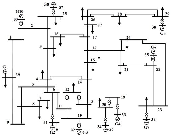
Figure 1.
New England IEEE thirty-nine-bus system [35].
For the IEEE 39-bus system, also known as the New England Power System, there are several more significant line outages. Among critical line outages, the outage of line 16–17 is particularly significant, as it connects major buses, potentially causing severe voltage drops and overloading adjacent lines. Similarly, the outage of line 6–11 leads to a substantial redistribution of power flow, increasing the risk of line overload and voltage instability. The loss of line 4–14 poses challenges to system stability by increasing reactive power demand and potentially causing voltage collapse. Lastly, the outage of line 1–2, which connects key generation buses, can result in generator tripping and islanding of system segments. These scenarios are extensively analyzed to evaluate their effects on system stability, voltage constraints, and the likelihood of cascading failures, providing insights into robust grid operation and planning.
4.2. PV Models for Replaced Generators
These terms refer to the control and protection settings of power systems. Pqflag sets the priority between the reactive (0) and active (1) current. Xc is the reactance used for line drop compensation, measured in per unit (pu) on the machine base (mbase). Qmx and Qmn define the maximum and minimum changes in reactive power due to voltage droop response, respectively, also in pu on mbase. V0 and V1 are the lower and upper limits of the deadband for the voltage droop response. Dqdv characterizes the voltage droop response, while fdbd is the overfrequency deadband for the governor response, measured in pu deviation. Ddn represents the down-regulation droop gain in pu on mbase, and Imax is the apparent current limit in pu on mbase. The voltage tripping thresholds are set by and , with Vrflag indicating the fraction of generation that can reconnect after voltage tripping. The frequency tripping thresholds are defined by , and , with frflag indicating the fraction of generation that can reconnect after frequency tripping. Tg and Tf are the time constants for inverter current lag and frequency measurement lag, respectively. Vtmax is the voltage limit for high-voltage clamp logic. Lvpnt1 and lvpnt0 are breakpoints for low-voltage active current management. Qmin and accel are terms for high-voltage reactive current management, not used by PowerWorld.
Table 1 presents the generator reactance parameters, which are essential for subtransient and transient stability analysis in the IEEE 39-bus system. The parameters (transient reactance) and (subtransient reactance) govern the generator’s short-term and very short-term responses to disturbances, influencing fault current levels and dynamic stability. Similarly, and determine the quadrature-axis dynamics, which are crucial for modeling power oscillations. The armature reactance and synchronous reactance affect steady-state performance and power flow calculations. These parameters collectively enable accurate evaluation of generator performance during faults, aiding in the prevention of cascading failures in interconnected grids.

Table 1.
Generator reactance parameters.
Table 2 provides the generator time constants, which are critical to modeling the dynamic behavior of the IEEE New England 39-bus system. The direct axis time constants, and , along with their quadrature axis counterparts, and , define the subtransient and transient response characteristics of the generator. These parameters are essential to understanding how quickly a generator can stabilize following a disturbance. The inertia constant, H, quantifies the stored rotational energy of the generator and its ability to resist frequency changes, which plays a key role in the overall stability of the system. Together, these time constants and inertia parameters enable precise analysis of generator dynamics, supporting the development of robust strategies for fault mitigation and grid resilience.
Table 2.
Generator time constants.
Table 3 provides the machine data for generators in the IEEE New England 39-bus system, including their real power generation (), maximum and minimum real power limits (), reactive power limits (), and MVA capacity. These parameters are crucial to understanding the operational constraints and power capabilities of each generator. The and define the range of active power that can be supplied under normal operating conditions, while and represent the ability of the generator to supply or absorb reactive power for voltage control. The MVA capacity provides the apparent power rating, which is critical for assessing the generator’s contribution to grid stability and reliability. These data are essential for load flow analysis, stability studies, and system planning.
Table 3.
Machine data with MVA capacity.
Figure 2 illustrates the time constant values for the 10 generators in the IEEE 39-bus system. In various studies, a combination of MVA and time constant is often employed to represent system dynamics. In cases where the time constant is reduced by a factor of 10, the MVA capacity is typically scaled by a factor of 10 to maintain the same system behavior. This adjustment ensures that the system’s inertia, which is a product of the time constant and the MVA capacity, remains consistent. The reciprocal relationship between the time constant and the MVA capacity provides a means of controlling the intensity of changes in the system inertia, thereby facilitating the preservation of system stability under different operating conditions.
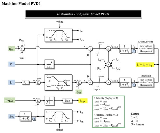
Figure 2.
Replaced low-inertia generators with this PVD1 PV model [36].
The dynamic data provided in [34] were insufficient to accurately model the generators required for detailed EMT simulation studies. Consequently, additional parameters, including subtransient data, were obtained from [37] to ensure comprehensive modeling.
The analysis presented in Section 2 and Section 3 reveals that the subtransient and transient parameters play a pivotal role in determining the CCT of the system. Specifically, the results highlight that increased PV integration can lead to a reduction in the effective inertia of the system, thereby affecting the transient stability margins. Furthermore, this study identified that certain generators are more susceptible to the effects of PV integration, depending on their electrical distance from the PV sources, their inherent inertia, and their subtransient characteristics. By quantifying these relationships, the analysis provides valuable information on the mechanisms through which PV integration influences transient stability. This understanding is crucial for power system operators and planners, as it allows for the development of strategies to mitigate potential stability issues and improve the resilience of power systems in the face of the growing integration of variable distributed energy.
5. IEEE 39-Bus Performance Under Different Photovoltaic Penetration Levels
In this results section, we investigate the impact of integrating photovoltaic (PV) systems to enhance solar energy integration by systematically replacing low-inertia generators. The study begins with the replacement of the generator at bus 37 (GEN 8), identified as having the third-lowest inertia (), resulting in a PV integration of (case 1). Subsequent replacements of generators at bus 34 (GEN 5, ), bus 36 (GEN 7, ), and bus 32 (GEN 3, ) increased PV integration progressively to (case 2), (case 3), and (case 4). By case 5, the integration of PV systems at bus 33 (GEN 4, ) achieved a total PV integration of .
This gradual increase in PV integration enabled the research to determine CCT for various outages under progressively reduced inertia conditions. It also provided insights into the proposed subtransient and transient sensitivity parameters across different inertia scenarios. As synchronous generators were replaced, their corresponding base MVA capacities were removed, resulting in proportional reductions in system inertia (), which decreased from (case 0) to (case 5), as seen in Table 4. These reductions directly affected the dynamic response of the system to faults, leading to shorter CCTs with increasing integration of PV, as detailed in Table 5.
Table 4.
System inertia constants () and PV integration for various cases.
Table 5.
Comparing original bus and modified bus CCT (S) for different outages under different PV integration scenarios.
The total simulation time is set to 10 s. A pre-fault steady-state condition runs for 1 s. The fault is applied based on the selected outage scenario and is used to determine the Critical Clearing Time (CCT). The post-fault trajectory is simulated up to the 10 s mark to assess system stability.
5.1. Subtransient and Transient Sensitivity Parameters for Generators When Changing PV Integration
Table 4 compares the system inertia constants () and PV integration levels for various cases in the IEEE New England 39-bus system. Initially, low-inertia generators, such as GEN 8 at bus 37 () and GEN 5 at bus 34 (), were replaced with PVD1-controlled PVs. These replacements resulted in a modest reduction of from in the original system to (case 1) and further to (case 2). This approach minimized the impact on system stability, as low-inertia generators contribute less to overall system inertia.
Subsequently, generators with relatively higher inertia, such as GEN 7 on bus 36 () and GEN 3 at bus 32 (), were replaced in cases 3 and 4. These replacements increased the integration of PV to and , respectively, while reducing to and .
Finally, cases 6 and 7 replaced bus 35 (GEN 6, ) and bus 38 (GEN 9, ) with PVs, focusing on assessing how PV generators respond during outages of high-inertia generators. These cases maintained similar values ( and ), since they represent scenarios where the outages of the PV generator are studied rather than increasing the integration of the PV.
This table highlights how the strategic replacement of low- and high-inertia generators affects , demonstrating the importance of generator selection and control strategies in maintaining system stability as PV integration increases.
Table 5 compares the CCT for various outages in the IEEE 39-bus system under different PV integration scenarios. As PV integration increases (from case 0 to case 5), the system inertia , as highlighted in the previous tables, decreases from in case 0 to in case 5. This reduction in system inertia directly results in shorter CCTs, indicating a decline in system stability. For instance, the CCT for the branch 2–3 contingency reduces from in case 0 to in case 5, demonstrating the impact of reduced inertia on transient stability. Similar trends are observed for other branches, such as branches 4–14 and 6–11, where CCTs decrease significantly with higher PV integration.
In particular, anomalies are observed in certain cases. For example, the CCT for the branch 23–24 contingency shows a slight recovery (from to ) in case 5. This may be attributed to the stabilizing effects of neighboring PV generators, which, under certain conditions, provide localized voltage support or alter power flow patterns to mitigate instability. Furthermore, for the bus 35 outage, the CCT increases from in case 4 to in case 5, despite the overall reduction in . These deviations may stem from localized stabilizing effects introduced by PV placement. Specifically, the replacement of the generator on bus 32 in case 4, which is electrically closer to branch 23–24, may reduce local fault current contributions or change the impedance profile, thus improving the transient stability in that area. Unlike earlier PV replacements at buses 37, 34, and 36, this topological change alters the dynamic behavior of nearby contingencies. These observations underscore the importance of not just the quantity but also the location and coordination of the PV integration, as they critically influence the stability outcomes. These anomalies suggest that the placement and control of PV generators, highlighted in the latter, play a critical role in the stability results.
Further insights can be drawn for cases involving unstable generators, such as branches 25–26 and 28–29, where increasing PV integration leads to generator instability in cases 4 and 5. These results underscore the trade-offs between renewable integration and system stability, emphasizing the importance of strategic PV placement and advanced control systems to address transient stability challenges in high-photovoltaic systems.
5.2. Comparative Analysis of the Original Bus and PV-Integrated Bus
This study investigates the impact of integrating a photovoltaic system on the stability of the power system using the IEEE 39-bus system in Power World [38]. Several three-phase line faults were conducted on the bus to compare the CCT between the original and modified PV-integrated bus. All faults are fault-on-trajectory without clearing the fault to fully comprehend subtransient and transient responses.
5.3. Analyzing Transient Responses for Different Outages When Bus 37 Generator Is Replaced by PVD1-Controlled PV Generators, or Case 1
In scenario 1, the generator with the least inertia, located in the 37-bus system, was replaced by PVD1-controlled PV generators that operate with zero inertia. Figure 3 illustrates this setup in Power World. To assess the system’s performance during transient and steady states, three different outages were examined: two related to the lines and one affecting a bus.
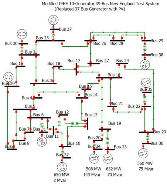
Figure 3.
Modified IEEE 39-bus system after replacing the 37th bus generator with a PV generator.
Figure 4 illustrates the current trajectories of generators following the replacement of the 37th bus generator with a photovoltaic generator, during a 2–3 balanced three-phase solid outage. These situations were chosen to investigate the system’s subtransient and transient response in the initial cycles, as well as its steady-state behavior over up to 5 s. Among the generators, bus 37 (generator 8) had the lowest magnitudes of the fault current, while bus 34 (generator 5) showed the most stable response to the fault current during the outages. In contrast, generator 3 caused oscillatory waveforms in the grid. Due to these modifications, the CCT was reduced from 0.255 s to 0.247 s, suggesting a slight decrease in system stability under these circumstances. The sharp step in bus-30 gen (blue) is due to its proximity to the fault and the slack bus, creating a low-impedance path with minimal transient response. Limited dynamic modeling also causes a near-instantaneous current jump.
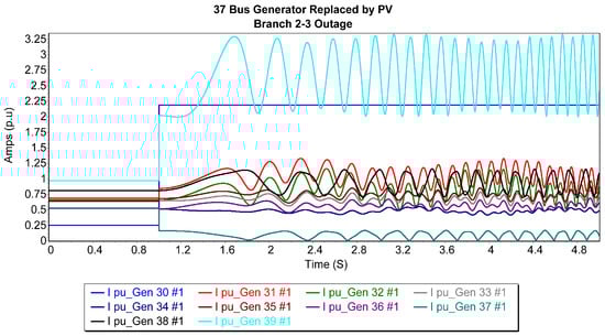
Figure 4.
Generator current trajectories after replacing the 37th bus generator with a PV generator for 2–3 3P balanced fault.
Figure 5 presents the current trajectories of the generators after replacing the 37th bus generator with a photovoltaic generator during a balanced three-phase outage near bus 15 on the 15–16 line. Bus 37 (generator 8) exhibited the lowest fault current magnitudes, while buses 34 and 36 (generators 5 and 7) demonstrated the most stable fault current responses. In contrast, generators 1 and 10 exhibited the most oscillatory waveforms, introducing significant turbulence into the grid. These modifications led to a reduction in the CCT from 0.231 s to 0.211 s, indicating a slight decline in system stability under these conditions.
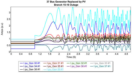
Figure 5.
Generator current trajectories after replacing the 37th bus generator with a PV Generator for 15–16 3P balanced fault.
In the setup of case 1, Figure 6 illustrates the current trajectories of the generators after replacing the 37th bus generator with a photovoltaic generator during a balanced three-phase outage on bus 35. Among the generators, bus 39 (generator 1) recorded the highest fault current magnitudes, while bus 34 (generator 5) exhibited the most stable fault current response. Conversely, generators 1, 8, and 10 exhibited notably oscillatory waveforms, contributing to substantial grid turbulence. This led to a decrease in the CCT from 0.246 s to 0.239 s, indicating a slight drop in the system’s stability in these circumstances.
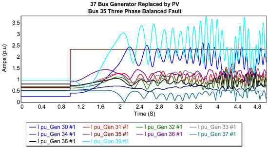
Figure 6.
Generator current trajectories after replacing the 37th bus generator with a PV generator for 35-bus 3P balanced fault.
In the modified system where the synchronous generator at the 37-bus was replaced by a photovoltaic (PV) generator, references for rotor angle (Figure 7) and rotor speed (Figure 8) were initially included for comparison. However, the rotor dynamic responses—specifically the angular position and speed trajectories—remain nearly identical to those of the original system. This indicates that the electromechanical behavior of the network has not significantly changed due to the generator replacement.
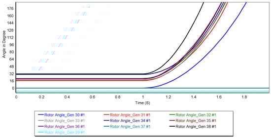
Figure 7.
Rotor angle for other generators when the 37th bus generator is replaced by PV and bus 2–3 3P fault.
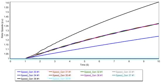
Figure 8.
Rotor speed for other generators when 37th bus generator is replaced by PV and bus 2–3 3P fault.
5.4. Analyzing Transient Responses for Different Outages When Bus 37, 34 Generators Are Replaced by PV Generators, or Case 2
In case 2, the transient responses were analyzed after replacing the bus 37 and bus 34 generators with photovoltaic generators. This replacement resulted in a system inertia constant () of 95.35 s and a photovoltaic integration of 17.3%. Different outages, including line and bus faults, were examined to observe the system’s transient behavior during the initial cycles and its steady-state response over a duration of 5 s. The incorporation of zero-inertia photovoltaic generators increased oscillations in certain generators, reduced CCT, and led to a slight decrease in overall system stability.
In the configuration of case 2, Figure 9 presents the current trajectories of the generators after the replacement of the 37th and 34th bus generators with a photovoltaic (PV) generator during a balanced solid three-phase outage on branch 2–3. Bus 39 (generator 1) was observed to exhibit the highest magnitudes of fault current among all generators, whereas buses 35 and 36 (generators 6 and 7) displayed the most consistent and stable responses to fault currents. On the contrary, generators 1, 2, and 9 demonstrated significant oscillatory waveforms, which introduced considerable disturbances within the power grid. These alterations resulted in a decrease in the CCT from 0.247 s to 0.196 s, suggesting a marginal decline in system stability under these circumstances.
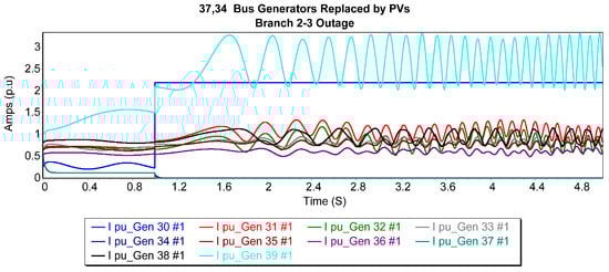
Figure 9.
Generator current trajectories after replacing the 37th and 34th bus generators with a PV generator for 2–3 3P balanced fault.
Figure 10 illustrates the current trajectories of generators after replacing the 37th and 34th bus generators with photovoltaic (PV) generators during a balanced solid three-phase outage on branches 15–16. Among the generators, buses 34 and 37 (generators 5 and 8) exhibited the lowest fault current magnitudes, approaching zero, while buses 35 and 36 (generators 6 and 7) displayed the most stable fault current responses. In contrast, generators 1 and 10 demonstrated significant oscillatory waveforms, introducing considerable turbulence into the grid. These changes reduced the CCT from 0.211 s to 0.186 s, signifying a slight reduction in system stability under these conditions.
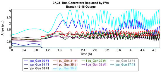
Figure 10.
Generator current trajectories after replacing the 37th and 34th bus generators with a PV generator for 15–16 3P balanced fault.
Figure 11 shows the current trajectories of the generators in case 2, where a photovoltaic (PV) generator replaces the 37th bus generator during a balanced solid three-phase outage on bus 35. In particular, buses 34 and 37 (generators 5 and 8) recorded the lowest fault current magnitudes, near zero. In contrast, generator 1 exhibited highly oscillatory waveforms, causing significant turbulence in the grid, whereas the other generators showed varying levels of turbulence except for generators 5 and 8. These changes led to a reduction in the CCT from 0.239 to 0.184 s, marking a significant decrease compared to other outages in this case and indicating the highest decline in system stability during a trajectory fault.
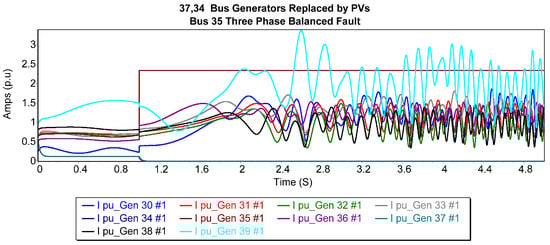
Figure 11.
Generator current trajectories after replacing 37th and 34th bus generators with a PV generator for 35-bus 3P balanced fault.
5.5. Analyzing Transient Responses for Different Outages When Bus 37, 34, 36 Generators Are Replaced by PV Generators, or Case 3
In case 3, the transient responses were analyzed after replacing the bus 37, bus 34, and bus 36 generators with photovoltaic generators. This configuration resulted in a system inertia constant () of 93.01 s and a photovoltaic integration of 26.5%. Several outages, including line and bus faults, were assessed to evaluate the system’s transient behavior during the initial cycles and its steady-state response over 5 s. The integration of additional zero-inertia photovoltaic generators further amplified oscillations in certain generators, reduced the CCT, and contributed to a notable decrease in the overall system stability.
In the setup of case 3, Figure 12 shows the fault current paths during a balanced solid three-phase outage on branches 2–3. Of all generators, bus 39 (generator 1) showed the highest fault current levels, while bus 37 (generator 8) maintained the most stable fault current behavior. In contrast, generator 1 exhibited significant oscillatory patterns, causing substantial disturbances to the grid. These circumstances reduced the CCT from 0.197 s to 0.177 s, indicating a 10.15% reduction in CCT due to the increased integration of PV of 26. 5% compared to case 2 (17.3%).
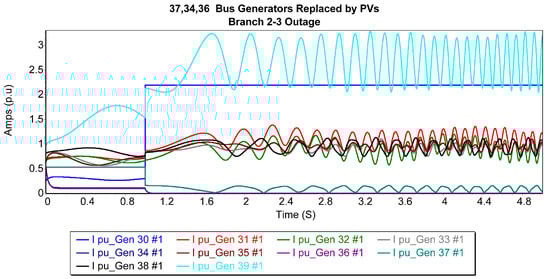
Figure 12.
Generator current trajectories after replacing 37th, 34th, and 36th bus generators with a PV generator for 2–3 3P balanced fault.
In case 3, Figure 13 depicts the fault current trajectories during a balanced, solid three-phase outage on branch 2–3. Bus 39 (generator 1) recorded the highest fault current levels among all the generators, while buses 35 and 33 (generators 4 and 6) showed the most stable fault current behavior. In contrast, generators 1 and 10 exhibited notable oscillatory patterns, introducing significant disturbances to the grid. These dynamics resulted in a considerable reduction in the CCT, which decreased from 0.186 to 0.141 s compared to case 2.
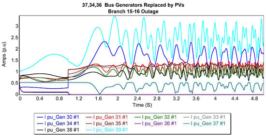
Figure 13.
Generator current trajectories after replacing 37th, 34th, and 36th bus generators with a PV generator, for 15–16 3P balanced fault.
In case 3, Figure 14 illustrates the trajectories of the fault current during a balanced solid three-phase outage at bus 35. The majority of generators, except generator 8, demonstrated significant turbulence, indicating a substantial impact on grid stability. These dynamics resulted in a relatively smaller reduction in Critical Clearing Time (CCT), decreasing from 0.184 to 0.173 s compared to case 2.
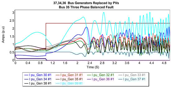
Figure 14.
Generator current trajectories after replacing 37th, 34th, and 36th bus generators with PV generator for 35-bus 3P balanced fault.
5.6. Analyzing Transient Responses for Different Outages When Bus 37, 34, 36, and 32 Generators Replaced by PV Generators, or Case 4
In case 4, the transient responses were analyzed after replacing the bus 37, bus 34, bus 36, and bus 32 generators with photovoltaic generators. This configuration led to a system inertia constant () of 90.22 s and a photovoltaic integration of 34.9%. Various outages, including line and bus faults, were examined to assess the system’s transient performance during the initial cycles and its steady-state response over a 5 s duration. Including additional zero-inertia PV generators further increased oscillations in specific generators, significantly reduced them, and resulted in a more pronounced decline in the overall stability of the system.
Figure 15 illustrates case 4 in the PowerWorld environment, showcasing the generator output settings that remained unchanged despite replacing the generators with photovoltaic (PV) generators in four different buses. The figure further depicts the current trajectories of the generators after this replacement, highlighting the transient behavior following these modifications.
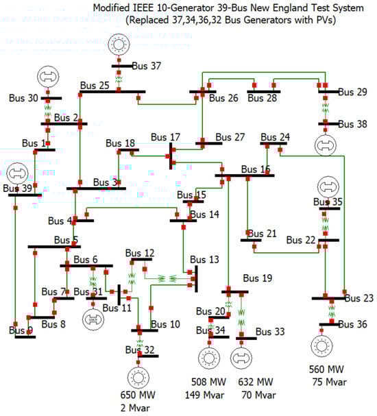
Figure 15.
Generator current trajectories after replacing the 37th, 34th, 36th, and 32nd bus generators with PV generators.
In the setup of case 4, Figure 16 shows the fault current paths during a balanced, solid three-phase outage on branch 2–3. Within the set of generators, generators 1 and 8 displayed the highest levels of fault current accompanied by oscillations, whereas generators 3, 5, and 7 exhibited the lowest fault current levels, approximately 0 pu. Furthermore, the CCT was decreased by a factor of approximately 2.41 relative to the original New England bus configuration (0.255 s) and by a factor of 1.67 in comparison to case 3 (0.177 s).
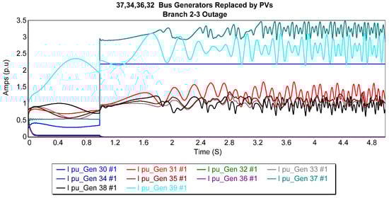
Figure 16.
Generator current trajectories after replacing the 37th, 34th, 36th, and 32nd bus generators with a PV generator for 2–3 3P balanced fault.
In the configuration of case 4, Figure 17 illustrates the fault current routes during a balanced, solid three-phase fault on branch 15–16, near bus 15. Of all the generators, generator 1 showed the highest fault current levels with fluctuations, whereas generators 3, 5, and 7 displayed the lowest fault currents (approximately 0 pu). The CCT (0.132 s) decreased by approximately 1.75 times compared to the original New England bus setup (0.231 s) and by approximately 1.07 times compared to case 3 (0.141 s).
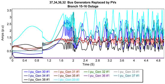
Figure 17.
Generator current trajectories after replacing the 37th, 34th, 36th, and 32nd bus generators with a PV generator for 15–16 3P balanced fault.
In the configuration of case 4, Figure 18 illustrates the fault current trajectories during a balanced, solid three-phase outage on bus 35. Among all the generators, generator 1 recorded the highest fault current levels accompanied by oscillations, whereas generators 3, 5, and 7 exhibited the lowest fault currents (approximately 0 pu). The CCT (0.096 s) was reduced by approximately 2.56 times compared to the original New England bus configuration (0.246 s) and by approximately 1.8 times compared to case 3 (0.173 s).

Figure 18.
Generator current trajectories after replacing 37th, 34th, 36th, and 32nd bus generators with a PV generator for 35-bus 3P balanced fault.
5.7. Analyzing Transient Responses for Different Outages When Bus 37, 34, 36, and 33 Generators Replaced by PV Generators, or Case 5
In case 5, the transient responses were analyzed after the replacement of the bus 37, bus 34, bus 36, and bus 33 generators with photovoltaic generators. This configuration resulted in a system inertia constant () of 87.15 s and a photovoltaic integration of 37.2%. A variety of outages, including line and bus faults, were investigated to evaluate the system’s transient behavior during the initial cycles and its steady-state response over a duration of 5 s. The incorporation of supplementary zero-inertia PV generators exacerbated oscillations in particular generators, further diminished the CCT, and contributed to a significant decline in the overall stability of the system.
In the setup of case 5, Figure 19 illustrates the fault current trajectories during a balanced, solid three-phase outage on branch 2–3. Among all the generators, generator 1 exhibited the highest levels of fault current with oscillations, while generators 4, 5, and 7 displayed the lowest fault currents, measuring around 0 pu. The CCT (0.084 s) was reduced by approximately 3.04 times compared to the original New England bus configuration (0.255 s) and by approximately 1.26 times compared to case 4 (0.106 s).
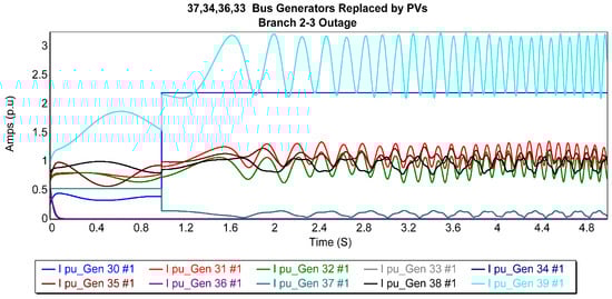
Figure 19.
Generator current trajectories after replacing the 37th, 34th, 36th, and 33rd bus generators with a PV generator for 2–3 3P balanced fault.
In the configuration of case 5, Figure 20 shows the paths of fault currents during a balanced solid three-phase failure on branch 15–16. Most of the generators exhibited fluctuations in their fault current paths, with generators 1 and 10 displaying the most significant oscillations. The CCT of 0.097 s was reduced by approximately 2.38 times relative to the initial bus configuration (0.231 s) and by about 1.36 times compared to case 4 (0.132 s).
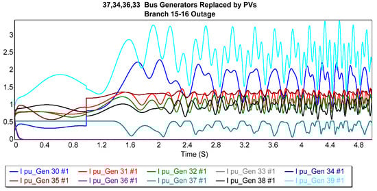
Figure 20.
Generator current trajectories after replacing the 37th, 34th, 36th, and 33rd bus generators with a PV generator for 15–16 3P balanced fault.
In the configuration of case 5, Figure 21 illustrates the fault current paths during a balanced, solid three-phase outage on bus 35. Most generators exhibited significant fluctuations in their fault current trajectories, and generator 6 exhibited relatively stable behavior. The CCT of 0.159 s represents a reduction of approximately 1.45 times relative to the original New England bus configuration, which was 0.231 s, and an increase of approximately 1.66 times when compared to case 4, measured at 0.096 s. This increase in CCT for the PV outage could be attributed to buses 33 and 36, which are neighboring PV buses that could influence the stability of the system under these conditions.
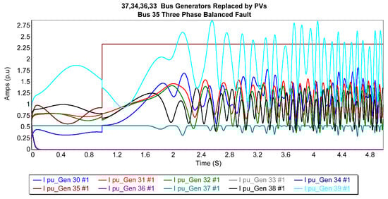
Figure 21.
Generator current trajectories after replacing the 37th, 34th, 36th, and 33rd bus generators with a PV generator for 35-bus 3P balanced fault.
5.8. Single Generator Fault-On Current Trajectories for Different Cases with Different PV Integrations
The subtransient and transient reactances and current magnitude changed after comparing the photovoltaic-integrated modified bus with the original system. This depends on the level of PV integration, which confirms the sensitivity parameters.
This analysis compares the short-circuit current trajectories of the 31-bus generator (generator 2) for the original New England bus configuration and scenarios where generators are replaced by PQ-controlled negative loads. The objective is to assess the sensitivity parameters of the system under these configurations. Figure 22 demonstrates the changes in generator current dynamics, emphasizing the impact of generator replacement on system behavior during faults.
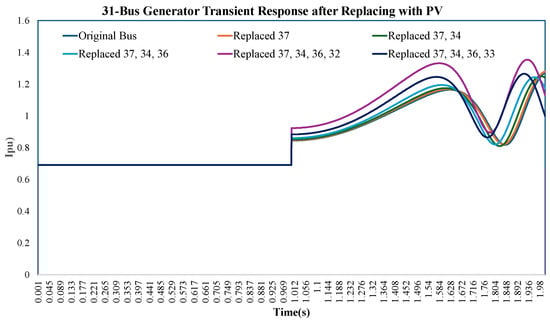
Figure 22.
31-bus generator or generator 2 short-circuit current magnitudes (fault-on) for original New England bus versus different generators replaced by a negative load.
Figure 23 represents the same generators and case studies; however, in this instance, the actual PVD1 PV model is used instead of the PQ-controlled negative load for PV replacements. An examination of this figure about the preceding one indicates that the fault-on current trajectory exhibits considerable similarity in both instances. However, it is observed that the PVD1 PV model induces certain oscillations in the steady-state response, thereby elucidating the disparities in dynamic behavior between the two models during and following the fault scenarios.
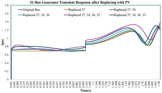
Figure 23.
31-bus generator short-circuit current magnitudes (fault-on) for original New England bus versus different PV-penetrated buses.
The scenario in Figure 24 examines the short-circuit current trajectories of the 35-bus generator (generator 6) across all five cases, including the original New England bus configuration, during a balanced three-phase outage on the 2–3 branch. In the original New England bus setup, the generator displays relatively stable fault current behavior due to the presence of synchronous generators with inherent inertia.
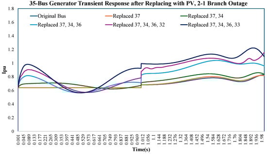
Figure 24.
35-bus generator short-circuit current magnitudes (fault-on) for original New England bus vs. different PV-penetrated buses for 2–3 branch outage.
In case 1, with a single generator replaced by a PV generator, slight oscillations begin to appear in the fault current trajectory. Case 2, which includes higher PV integration with multiple generators replaced, shows more pronounced oscillations and reduced fault current magnitudes. In case 3 and case 4, as additional zero-inertia PV generators are integrated into the system, the fault current trajectory demonstrates further disturbances, with notable oscillatory behavior in both the transient and steady-state phases. In case 5, the system dynamics for generator 6 are significantly impacted, with fluctuations in fault currents increasing and stability reducing even further.
This analysis across all scenarios underscores the incremental impact of enhanced PV integration on the fault response of the 35-bus generator, highlighting the difficulties associated with preserving system stability and dynamic performance as traditional synchronous generators are substituted by PV systems.
5.9. CCT Changes for PV Bus Generator Three-Phase Faults: Cases 6 and 7 Explored
Table 6 presents the CCT comparisons for specific generator buses in the IEEE New England 39-bus system when synchronous generators are replaced with photovoltaic (PV) systems. The table highlights the original New England bus CCT (prior to PV integration), the modified bus CCT (post-PV integration), and the percentage increase in CCT. This analysis demonstrates how PV integration, under certain conditions, can enhance transient stability.
Table 6.
Comparing original bus and modified bus CCT for PV generators.
For the generator at bus 35, the CCT increases from to , resulting in a improvement. This significant increase indicates that replacing the synchronous generator at bus 35 with a PV system improved stability, likely due to improved localized voltage regulation and power flow adjustments provided by the PV system’s control mechanisms. This result underscores the potential benefits of PV integration in strategically chosen locations.
At bus 37, the CCT improves from to , representing a notable increase. The substitution of the generator on bus 37 with a PV system appears to exert a particularly intense stabilizing influence. This outcome can be attributed to the central location of the bus within the network, allowing the PV system to supply essential reactive power support and mitigate power imbalances in adjacent buses. At bus 38, the Critical Clearing Time (CCT) increases from to infinite time, indicating that the system can now withstand the fault indefinitely without losing stability. This finding indicates that replacing the generator on bus 38 with a PV system eradicated the critical fault condition in the modeled scenario. The PV system might have rectified local bottlenecks or decreased current contributions to the fault, thereby significantly stabilizing the system under fault conditions.
These results highlight the importance of localized stability improvements achieved through PV integration. Although photovoltaic systems generally reduce system inertia, as observed in previous tables, their ability to provide voltage and frequency support can result in enhanced transient stability when strategically placed. The exceptional improvement at bus 38 further demonstrates the influence of network topology on the effectiveness of PV integration. This analysis underscores the need for careful planning in PV deployment to balance the integration of variable distributed energy with the stability of the grid.
Figure 25 depicts the stabilization of rotor speed across all generators subsequent to a three-phase fault, following the substitution of the 38th bus generator with a PV generator.Despite the fault, the system achieves a steady state, suggesting an infinite CCT, but making fault detection more challenging. The zero-inertia nature of the PV generator alters the transient response, affecting the stability dynamics and the sensitivity to fault detection.
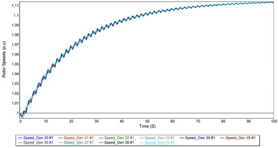
Figure 25.
Rotor speeds for other generators when 38th bus generator is replaced by PV and 3P fault.
Figure 26 shows the rotor angle trajectories when the 38th bus generator is replaced by a PV generator, followed by a sustained three-phase fault. Unlike conventional generators, the zero-inertia nature of the PV generator causes the rotor angle dynamics to stabilize to new steady-state values even during the fault. The fault-on trajectory converges towards these stable values, demonstrating the system’s capacity to withstand the fault without losing stability, albeit with a markedly altered response in comparison to conventional synchronous generators.
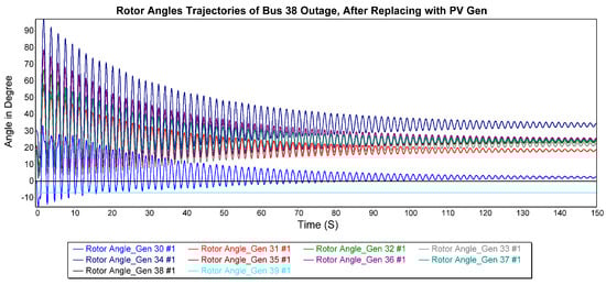
Figure 26.
Rotor angles for other generators when 38th bus generator is replaced by PV and 3P fault.
5.10. Determining Sensitivity Parameters
To illustrate, the computation of the ratio of to involves dividing by , which results in an approximate value of . Subsequently, the natural logarithm of this ratio is calculated, yielding . Afterward, the ratio of to is determined by dividing by , which yields an approximate value of . The natural logarithm of the latter ratio is then computed as . Finally, the division of these logarithmic values, by , yields the value of , in accordance with Equation (14).
The sensitivity of Generator 2 to PV integration, as illustrated in Figure 27, exhibits a clear downward trend over time. At an initial photovoltaic integration of 8.9%, the sensitivity is minimal, indicating negligible influence of photovoltaic systems on generator dynamics. However, as the integration increases to 17.3%, the sensitivity increases significantly, demonstrating the pronounced impact of intermediate levels of photovoltaic integration. Beyond this point, at higher integration levels such as 37.2%, the sensitivity increases at a steeper rate. This upward trend underscores the nonlinear relationship between PV integration and generator sensitivity, with the most pronounced impacts observed at intermediate penetration levels.
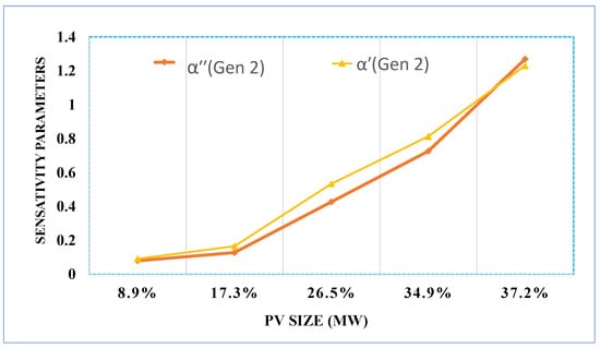
Figure 27.
31-bus generator (gen 2) inertia sensitivity parameter analysis for different PV-penetrated buses.
As shown in Figure 28, the sensitivity of Generator 6 to PV integration exhibits a distinct upward trend over time, with its magnitude notably higher than that of Generator 2. This is likely due to the replacement of several neighboring generators with PV systems, indicating that generator 6’s response is strongly influenced not only by the overall PV integration but also by the specific location of PV generators within the system. The sensitivity increases steadily as the integration of PV increases, reaching its peak around 35% integration, reflecting the significant impact of both system inertia and generator positioning. However, beyond this point, the sensitivity of generator 6 begins to decline. This decrease is driven by the replacement of neighboring synchronous generators with PV systems, which diminishes the local system’s dynamic support and lowers generator 6’s sensitivity to further PV integration. In contrast to the continued upward trend observed for generator 2, this behavior underscores the influence of local system topology and generator placement, leading to a downward trend in sensitivity at high levels of PV penetration for generator 6.
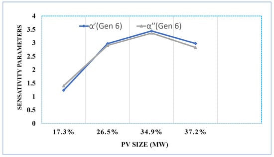
Figure 28.
35-bus generator (gen 6) inertia sensitivity parameter analysis for different PV-penetrated buses.
6. Conclusions and Future Work
This study examines the impact of the integration of photovoltaic (PV) systems to enhance the integration of solar energy in the IEEE 39-bus system by systematically replacing several generators with the lowest inertia. Although conventional transient stability parameters, such as CCT, are widely studied in the context of PV integration, the explicit relationship between inertia and parameters such as subtransient and transient reactances and time constants remains less explored. This paper addresses this gap by focusing on reactance sensitivity, which significantly influences the transient period. The analysis considers sensitivity parameters for both subtransient and transient responses, investigating their variations with changes in system inertia resulting from increasing PV integration. The results indicate that higher-inertia generators are more affected by proportional inertia changes than low-inertia generators. The sensitivity analysis of the transient reactance of the conventional generator revealed positive correlations with changes in inertia, while for photovoltaic generators, the sensitivity parameters exhibited negative values during balanced three-phase fault conditions. These findings underscore the critical role of reactance sensitivity in evaluating transient stability, particularly in systems undergoing significant integration of variable distributed energy. CCT for both original and modified buses under varying levels of integration of PV, as presented in Table 5, demonstrates a general decrease in CCT with increasing integration of PV. This reduction ranges from to , depending on the location of the outage and proximity to high- or low-inertia generators. The analysis shows a clear inverse relationship between PV penetration and system stability, with CCT consistently declining as PV share increases. For example, CCT drops by approximately 67% when PV integration reaches 37.2%. On average, this corresponds to a 1.8% reduction in CCT per 1% PV increase, emphasizing the sensitivity of transient stability to reduced inertia. Buses located closer to high-inertia generators, such as generator 1 (bus 39, ), experienced smaller reductions in CCT, reflecting the stabilizing influence of these generators. In contrast, buses adjacent to generators with low inertia, such as generator 2 (bus 31, ), exhibited more significant reductions in CCT, highlighting the vulnerability introduced by reduced system inertia. The calculated subtransient and transient inertia sensitivity parameters further explain these observations. Buses near high-inertia generators exhibited lower sensitivity to changes in inertia, whereas those near low-inertia generators showed higher sensitivity. In particular, in some scenarios, the energy provided by low-inertia photovoltaic systems is insufficient to reach the critical energy threshold of the system during disturbances, resulting in fault survival and an effectively infinite CCT. However, in other cases, this reduced inertia leads to instability, with generators failing to remain synchronized after faults. Although PV integration improves local generation performance, it can adversely affect the fault response and dynamic stability of the overall power system, especially conventional synchronous generators. This discrepancy underscores the critical need to balance the integration of renewables with the stability of the system. Evaluating transient stability parameters, such as CCT and reactance sensitivity, is essential for designing effective control strategies to mitigate the impacts of PV integration while maintaining reliable grid operation.
Future research will extend this study by examining subtransient and transient time constants during fault conditions to understand dynamic system behavior better. Furthermore, future studies will incorporate mitigation strategies such as adding synthetic inertia via inverter-based resources, tuning PV inverter control schemes (e.g., current limiting and PLL damping), and evaluating the stabilizing potential of FACTS devices. These efforts aim to develop a more comprehensive and practically applicable framework to improve the stability of the power system in high-renewable scenarios.
Author Contributions
Conceptualization, R.M., X.F. and M.B.-I.; methodology, R.M.; software, R.M. and X.F.; validation, R.M., X.F. and M.B.-I.; formal analysis, R.M., X.F. and M.B.-I.; investigation, R.M., X.F. and M.B.-I.; resources, R.M. and M.B.-I.; data curation, R.M. and C.H.; writing—original draft preparation, R.M. and C.H.; writing—review and editing, R.M., X.F. and M.B.-I.; visualization, R.M., X.F. and M.B.-I.; supervision, X.F. and M.B.-I.; project administration, X.F. and M.B.-I. All authors have read and agreed to the published version of the manuscript.
Funding
This research received no external funding.
Data Availability Statement
The data are contained within the article.
Acknowledgments
The authors gratefully acknowledge the administrative and technical support provided by the University of Nevada, Reno, particularly the Department of Electrical and Biomedical Engineering, which was instrumental in facilitating this research. Special thanks to the faculty, staff, and peers for their insightful discussions, constructive feedback, and encouragement throughout the project.
Conflicts of Interest
The authors declare no conflicts of interest.
References
- Makolo, P.; Zamora, R.; Lie, T.T. The role of inertia for grid flexibility under high penetration of variable renewables: A review of challenges and solutions. Renew. Sustain. Energy Rev. 2021, 147, 111223. [Google Scholar] [CrossRef]
- Prabhakar, K.; Jain, S.K.; Padhy, P.K. Inertia estimation in modern power system: A comprehensive review. Electr. Power Syst. Res. 2022, 211, 108222. [Google Scholar] [CrossRef]
- Martinez-Velasco, J.A. Power System Transients: Parameter Determination; CRC Press: Boca Raton, FL, USA, 2017. [Google Scholar]
- Senyuk, M.; Safaraliev, M.; Kamalov, F.; Sulieman, H. Power system transient stability assessment based on machine learning algorithms and grid topology. Mathematics 2023, 11, 525. [Google Scholar] [CrossRef]
- Golpira, H.; Román-Messina, A.; Bevrani, H. Renewable Integrated Power System Stability and Control; John Wiley & Sons: Hoboken, NJ, USA, 2021. [Google Scholar]
- Hingu, C.; Fu, X.; Vangala, P.; Mishan, R.; Fajri, P. 32-Bit Fixed and Floating-Point Hardware Implementation for Enhanced Inverter Control: Leveraging FPGA in Recurrent Neural Network Applications. IEEE Access 2024, 12, 111097–111110. [Google Scholar] [CrossRef]
- Hingu, C.; Fu, X.; Mishan, R.; Kim, T. PWM-Based Hardware Authentication for Smart Inverters: Detecting Counterfeit Inverter through Transient Response Analysis. In Proceedings of the 2024 IEEE Energy Conversion Congress and Exposition (ECCE), Phoenix, AZ, USA, 20–24 October 2024; pp. 1–6. [Google Scholar]
- Mishan, R.; Fu, X.; Hingu, C.; Fajri, P. Analyzing frequency spectrum and Total Harmonic Distortion for high switching frequency operation of GaN-based filter-less multilevel cascaded H-bridge inverter. e-Prime-Adv. Electr. Eng. Electron. Energy 2025, 11, 100906. [Google Scholar] [CrossRef]
- Hingu, C.; Fu, X.; Saliyu, T.; Hu, R.; Mishan, R. Power-Optimized Field-Programmable Gate Array Implementation of Neural Activation Functions Using Continued Fractions for AI/ML Workloads. Electronics 2024, 13, 5026. [Google Scholar] [CrossRef]
- Yagami, M.; Kimura, N.; Tsuchimoto, M.; Tamura, J. Power system transient stability analysis in the case of high-penetration photovoltaics. In Proceedings of the 2013 IEEE Grenoble Conference, Grenoble, France, 16–20 June 2013; pp. 1–6. [Google Scholar] [CrossRef]
- Tamrakar, U.; Galipeau, D.; Tonkoski, R.; Tamrakar, I. Improving transient stability of photovoltaic-hydro microgrids using virtual synchronous machines. In Proceedings of the 2015 IEEE Eindhoven PowerTech, Eindhoven, The Netherlands, 29 June–2 July 2015; pp. 1–6. [Google Scholar]
- Eftekharnejad, S.; Vittal, V.; Heydt, G.T.; Keel, B.; Loehr, J. Impact of increased penetration of photovoltaic generation on power systems. IEEE Trans. Power Syst. 2012, 28, 893–901. [Google Scholar] [CrossRef]
- Mishan, R.; Egan, M.S.; Fu, X.; Hingu, C.; Fajri, P.; Ben-Idris, M. Assessing power profile characteristics in solar PV-storage integrated electricity markets: A quantitative study. e-Prime Adv. Electr. Eng. Electron. Energy 2024, 9, 100684. [Google Scholar] [CrossRef]
- Papadopoulos, P.N.; Milanović, J.V. Probabilistic Framework for Transient Stability Assessment of Power Systems with High Penetration of Renewable Generation. IEEE Trans. Power Syst. 2017, 32, 3078–3088. [Google Scholar] [CrossRef]
- Mohamed, S.R.; Jeyanthy, P.A.; Devaraj, D. Investigation on the impact of high-penetration of PV generation on transient stability. In Proceedings of the 2017 IEEE International Conference on Intelligent Techniques in Control, Optimization and Signal Processing (INCOS), Srivilliputtur, India, 23–25 March 2017; pp. 1–6. [Google Scholar]
- Impram, S.; Nese, S.V.; Oral, B. Challenges of variable distributed energy penetration on power system flexibility: A survey. Energy Strategy Rev. 2020, 31, 100539. [Google Scholar] [CrossRef]
- Kilgore, L.A. Calculation of Synchronous Machine Constants-Reactances and Time Constants Affecting Transient Characteristics. Trans. AIEE 1931, 50, 1201–1213. [Google Scholar] [CrossRef]
- Zhang, W.; Wen, Y.; Chung, C.Y. Inertia security evaluation and application in low-inertia power systems. IEEE Trans. Power Syst. 2024, 40, 1725–1737. [Google Scholar] [CrossRef]
- Venikov, V.A. Transient Phenomena in Electrical Power Systems: International Series of Monographs on Electronics and Instrumentation; Elsevier: Amsterdam, The Netherlands, 2014; Volume 24. [Google Scholar]
- Guo, S. Improvements to Power System Dynamic Load Model Parameter Estimation. Ph.D. Thesis, University of Illinois at Urbana-Champaign, Champaign, IL, USA, 2017. [Google Scholar]
- Yap, K.Y.; Sarimuthu, C.R.; Lim, J.M.-Y. Virtual inertia-based inverters for mitigating frequency instability in grid-connected variable distributed energy system: A review. Appl. Sci. 2019, 9, 5300. [Google Scholar] [CrossRef]
- He, C.; He, X.; Geng, H.; Sun, H.; Xu, S. Transient stability of low-inertia power systems with inverter-based generation. IEEE Trans. Energy Convers. 2022, 37, 2903–2912. [Google Scholar] [CrossRef]
- Mishan, R.; Abdelkader, A.; Egan, M.; Ben-Idris, M. Impacts of High Penetration PV Systems on Power System Stability Parameters. In Proceedings of the 2023 IEEE Industry Applications Society Annual Meeting (IAS), Nashville, TN, USA, 29 October–2 November 2023; pp. 1–7. [Google Scholar]
- Mishan, R. Angular Stability Analysis of Parallel Connected Grid-following PV Inverters. In Proceedings of the 2023 IEEE Texas Power and Energy Conference (TPEC), College Station, TX, USA, 13–14 February 2023; pp. 1–6. [Google Scholar] [CrossRef]
- Alaraifi, S.; El Moursi, M.S. Design considerations of superconducting fault current limiters for power system stability enhancement. IET Gener. Transm. Distrib. 2017, 11, 2155–2163. [Google Scholar] [CrossRef]
- Kundur, P. Power system stability. Power Syst. Stab. Control 2007, 10, 7-1. [Google Scholar]
- Athay, T.; Podmore, R.; Virmani, S. A practical method for the direct analysis of transient stability. IEEE Trans. Power Appar. Syst. 1979, PAS-98, 573–584. [Google Scholar] [CrossRef]
- Saha, S.; Saleem, M.I.; Roy, T.K. Impact of high penetration of variable distributed energy sources on grid frequency behaviour. Int. J. Electr. Power Energy Syst. 2023, 145, 108701. [Google Scholar] [CrossRef]
- Tan, B.; Zhao, J.; Netto, M.; Krishnan, V.; Terzija, V.; Zhang, Y. Power system inertia estimation: Review of methods and the impacts of converter-interfaced generations. Int. J. Electr. Power Energy Syst. 2022, 134, 107362. [Google Scholar] [CrossRef]
- Mao, X.; Zhu, W.; Wu, L.; Zhou, B. Comparative study on methods for computing electrical distance. Int. J. Electr. Power Energy Syst. 2021, 130, 106923. [Google Scholar] [CrossRef]
- Kamwa, I.; Viarouge, P.; Mahfoudi, R. Phenomenological models of large synchronous machines from short-circuit tests during commissioning-a classical/modern approach. IEEE Trans. Energy Convers. 1994, 9, 85–97. [Google Scholar] [CrossRef]
- Vittal, V.; McCalley, J.D.; Anderson, P.M.; Fouad, A.A. Power System Control and Stability; John Wiley & Sons: Hoboken, NJ, USA, 2019. [Google Scholar]
- Gibson, S. Generator Short-Circuit Current. 1973. Available online: https://service.multiquip.com/files/2-20230808-083811.pdf (accessed on 30 March 2025).
- Pai, A. Energy Function Analysis for Power System Stability; Springer Science & Business Media: Berlin/Heidelberg, Germany, 1989. [Google Scholar]
- Yang, P.; Liu, F.; Wei, W.; Wang, Z. Approaching the transient stability boundary of a power system: Theory and applications. IEEE Trans. Autom. Sci. Eng. 2023, 20, 2268–2279. [Google Scholar] [CrossRef]
- PowerWorld Corporation. Machine Model PVD1. Available online: https://www.powerworld.com/WebHelp/Content/TransientModels_HTML/Machine%20Model%20PVD1.htm (accessed on 30 December 2024).
- Gomez Lezama, F.R. Prediction and Control of Transient Instability Using Wide Area Phasor Measurements. Ph.D. Thesis, University of Manitoba, Winnipeg, MB, Canada, 2011. [Google Scholar]
- Illinois Information Trust Institute, Grainger College of Engineering. 2025. IEEE 39-Bus System. Available online: https://icseg.iti.illinois.edu/ieee-39-bus-system/ (accessed on 20 March 2025).
Disclaimer/Publisher’s Note: The statements, opinions and data contained in all publications are solely those of the individual author(s) and contributor(s) and not of MDPI and/or the editor(s). MDPI and/or the editor(s) disclaim responsibility for any injury to people or property resulting from any ideas, methods, instructions or products referred to in the content. |
© 2025 by the authors. Licensee MDPI, Basel, Switzerland. This article is an open access article distributed under the terms and conditions of the Creative Commons Attribution (CC BY) license (https://creativecommons.org/licenses/by/4.0/).