Article

A Multimodal Interaction-Driven Feature Discovery Framework for Power Demand Forecasting

1
College of Computer Science and Electronic Engineering, Hunan University, Changsha 410082, China
2
Department of Engineering, King’s College London, London WC2R 2LS, UK
*
Author to whom correspondence should be addressed.
Energies 2025, 18(11), 2907; https://doi.org/10.3390/en18112907
Submission received: 14 March 2025 / Revised: 24 May 2025 / Accepted: 25 May 2025 / Published: 1 June 2025
(This article belongs to the Special Issue Optimization and Machine Learning Approaches for Power Systems)

Abstract

:
Power demand forecasting is a critical and challenging task for modern power systems and integrated energy systems. Due to the absence of well-established theoretical frameworks and publicly available feature databases on power demand changes, the known interpretable features of power demand fluctuations are primarily derived from expert experience and remain significantly limited. This substantially hinders advancements in power demand forecasting accuracy. Emerging multimodal learning approaches have demonstrated great promise in machine learning and AI-generated content (AIGC). In this paper, we propose, for the first time, a textual-knowledge-guided numerical feature discovery (TKNFD) framework for short-term power demand forecasting by interacting text modal data—a potentially valuable yet long-overlooked resource in the field of power demand forecasting—with numerical modal data. TKNFD systematically and automatically aggregates qualitative textual knowledge, expands it into a candidate feature-type set, collects corresponding numerical data for these features, and ultimately constructs four-dimensional multivariate source-tracking databases (4DM-STDs). Subsequently, TKNFD introduces a two-stage quantitative feature identification strategy that operates independently of forecasting models. The essence of TKNFD lies in achieving reliable and comprehensive feature discovery by fully exploiting the dual relationships of synonymy and complementarity between text modal data and numerical modal data in terms of granularity, scope, and temporality. In this study, TKNFD identifies 38–50 features while further interpreting their contributions and dependency correlations. Benchmark experiments conducted in Maine, Texas, and New South Wales demonstrate that the forecasting accuracy using TKNFD-identified features consistently surpasses that of state-of-the-art feature schemes by up to 36.37% MAPE. Notably, driven by multimodal interaction, TKNFD can discover previously unknown interpretable features without relying on prior empirical knowledge. This study reveals 10–16 previously unknown interpretable features, particularly several dominant features in integrated energy and astronomical dimensions. These discoveries enhance our understanding of the origins of strong randomness and non-linearity in power demand fluctuations. Additionally, the 4DM-STDs developed for these three regions can serve as public baseline databases for future research.

1. Introduction

Power sectors are experiencing fundamental transitions towards sustainability and decarbonization, resulting in a marked rise in grid complexity. Accurate forecasting of power demand is critical for planning and dispatching these complex power grids, as well as for facilitating policy formulation and decision-making in competitive integrated energy system (IES) markets. However, the increasing occurrence of extreme weather events and advancements in complementary energy storage technologies like batteries and compressed air, along with the emergence of new business models including demand-side management and large-scale aggregation [1,2], have considerably intensified the nonlinearity and stochasticity of power demand fluctuations. This has created formidable challenges for accurate short-term power demand forecasting (SPDF).
It is widely recognized that data and features set the upper bound for machine learning performance, while models and their algorithms merely approximate this limit. As forecasting models grow sophisticated, research on short-term power demand forecasting (SPDF) has evolved from merely analyzing power demand changes to investigating their sources and identifying underlying features. This paradigm shift is particularly significant for modern power systems [3]. The mechanisms driving power demand fluctuations remain unclear, leading to a lack of theoretical guidance for systematically exploring the factors influencing these fluctuations and their correlations. Feature engineering [4] and representation learning [5] have become key approaches for capturing features.
Feature engineering techniques generally encompass feature selection and feature extraction. In feature selection, three widely utilized methods are the filter, wrapper, and embedding approaches. The filter method [6] evaluates feature importance using statistical metrics such as variance, chi-square test, correlation coefficient, and mutual information. Recent advances have incorporated causal inference methods to identify both direct and indirect factors that influence power demand fluctuations, thereby enhancing feature interpretability. For instance, the Causal Graph Neural Network (CGNN) has been proposed to identify the causal relations between weather features (e.g., temperature, humidity, wind speed, diffuse flows, and general diffuse flows) and power demand [7]. However, these methods essentially function as a form of filter method, as they cannot discover previously unknown features. The wrapper method [8] consists of a search algorithm and a machine learning model that assesses candidate feature subsets based on model performance. Unlike the previous two methods, the embedding method [4] integrates feature selection directly into the learning algorithm, thereby performing simultaneous feature selection and forecasting. In feature extraction, technologies such as statistics and signal processing are commonly applied to extract the most representative attributes concealed within time-series data. For example, statistical measures such as mean, variance, and kurtosis are computed using a sliding window to capture periodicity and fluctuation patterns of the load (e.g., daily, weekly, and seasonal features). Methods such as Empirical Mode Decomposition (EMD) are employed to separate the trend, periodic, and residual components of the load. Fourier transform and wavelet analysis are utilized to extract load spectral features and identify both high-frequency noise and low-frequency trends. A novel feature extraction technique, termed knowledge-based systematic feature extraction, has been proposed to identify households with plug-in electric vehicles [9].
In fact, the feature engineering methods discussed above are fundamentally based on original feature sets that are manually built using expert knowledge and domain experience. This arises from the lack of public power demand databases containing sufficient potential influencing factors for feature identification through calculation and learning. Consequently, existing studies empirically consider one or several influencing factors—such as weather, calendar, and social or economic indicators—as the original feature sets for selection and extraction. Weather is regarded as the most dominant factor affecting power demand change [7,10,11,12]. Numerous research efforts have selected weather-related factors—such as temperature, humidity, and precipitation—candidate features. For example, Ref. [13] studied the impact of different durations of moving average temperature and hysteresis temperature on SPDF accuracy and introduced the concept of the power demand neighbor effect. However, research has shown that weather is not the sole determinant of power demand fluctuation. Examining the characteristics of holiday power demand fluctuation, Ref. [14] concluded that the fluctuation pattern on holidays differs from that on non-holidays. Given that historical-specific data are relatively scarce, they proposed a transfer learning model to leverage data from neighboring cities. Ref. [15] trained models in specific situations—such as vacations and weekends—with the aim of enhancing SPDF accuracy during special event days. They observed that holiday data exhibit strong natural randomness, which profoundly affects SPDF. Ref. [16] explored the correlation between heating, gas, and power demands and designed a novel hybrid neural network for SPDF. Their research illustrates that a strong coupling exists between gas load and power demand, and incorporating gas load data could improve SPDF accuracy. Ref. [17] investigated the temporal dynamic coupling characteristics of load series and built an extended feature set. In general, the total number of original features currently derived from expert experience is quite limited, resulting in insufficient data prerequisites for feature selection and extraction methods to perform their intended functions. Feature engineering methods for power demand forecasting remain immature and necessitate further advancement [3].
Representation learning is a different approach from feature engineering. Without reliance on manually designed features, representation learning automatically learns and extracts useful feature representations from raw data. Furthermore, representation learning is data-driven rather than driven by prior knowledge. It enables models to uncover features directly from data, thereby significantly enhancing the performance of downstream tasks such as time-series prediction. Deep learning models are widely used in representation learning. For example, Ref. [18] proposed a multivariate, multistep forecasting framework based on temporal convolution networks (TCNs) for residential load. Utilizing TCNs’ causal and dilated convolutions, this study tackled challenges in capturing long-range dependencies in highly damaged data. Ref. [19] presented a spatial–temporal embedding graph neural network (STEGNN) for short-term load forecasting. This model constructs directed static and dynamic graphs and utilizes exponential moving average graph convolutional networks (EMA-GCNs) to capture spatial dependencies among electricity users. It also introduced trainable temporal embeddings to capture periodicity. The STEGNN has demonstrated high accuracy across multiple real-world datasets. Ref. [20] introduced a multistep electric vehicle charging load forecasting model based on an Autoformer variant (TDformerBCMG). This model utilizes TCN to extract temporal features, enhances frequency features through the Discrete Cosine Transform, and integrates a Bayesian-optimized error correction module (BCMG) to refine predictions. TDformerBCMG excels in addressing the sparsity and periodicity of EV charging loads. However, these models exhibit limited interpretability during the feature extraction process, making it challenging to intuitively comprehend their internal decision-making logic. Features learned through these representation learning methods are often abstract, and it is hard to clearly interpret the relationship between features and load changes.
In summary, due to the absence of well-established theoretical frameworks and publicly available feature databases on power demand changes, the known interpretable features of power demand fluctuations are primarily derived from feature engineering that relies on expert experience and remains significantly limited. This substantially hinders advancements in power demand forecasting accuracy.
Recently, multimodal learning [21] has emerged as a promising research direction in machine learning and artificial intelligence, demonstrating widespread applications in fields such as computer vision, medical diagnosis, and AI-generated content. Multimodal learning typically encompasses multimodal alignment, multimodal fusion, and multimodal interaction. Multimodal alignment [22] establishes semantic correspondences across different data modalities, keeping them consistent in a shared semantic space. For example, CLIP [23] is a representative model of multimodal alignment that maps images and texts to aligned semantic spaces through contrastive learning to achieve cross-modal matching. Specifically, the dual-tower architecture encodes images and texts independently and then aligns the modalities through similarity calculation. The learning goal is to maximize the similarity of positive sample pairs and minimize the similarity of negative sample pairs. Finally, the aligned semantic space is used to adapt new tasks such as cross-modal retrieval. Multimodal fusion [24] integrates data from multiple sources and different modalities—such as audio, video, text, and others—to capture the diversity and completeness of multimodal data. This process entails extracting features from each modality using techniques like convolutional neural networks for images, spectral analysis for audio, and bag-of-words models for text. These features are subsequently fused to form a unified representation for collaborative learning and joint decision-making. Multimodal interaction [25] traditionally studies the process of interaction between humans and computing systems through multiple perceptual channels (such as voice, images, gestures, text, etc.) in order to enhance user experience, which emphasizes human–computer interaction. In recent years, multimodal interaction has begun to study the process and effect of information delivery and the interaction between different modal features in order to improve task performance. For example, Ref. [26] proposed that there are two semantic interaction patterns between text and image, complementary and substitutive, in which complementary interaction means that the information delivery of the two modal features jointly enhances the user’s understanding of the reviews, while substitutive interaction indicates that the information delivery of one modal feature may overwrite or weaken the value of the other. Accordingly, this study constructs an interaction pattern capture module, coordinates the contribution weights of the two modalities, and achieves significant optimization of review helpfulness prediction. We recognize that multimodal alignment, multimodal fusion, and contemporary multimodal interaction are all rooted in semantic associative relations across different modal spaces in terms of granularity, scope, and temporality, including but not limited to consistency/synonymy, hyponymy, complementarity, substitutability, and causality. By integrating and interacting with different modalities, it is possible to unlock a completely novel approach to feature discovery, moving beyond the traditional reliance on purely numerical data space in power systems.
Inspired by this, in the field of power demand forecasting, we select two modalities of data—text and numerical—for one-way interaction and propose a textual-knowledge-guided numerical feature discovery (TKNFD) framework. The text modal knowledge of power demand change is dispersed across various countries and regions worldwide, but has not yet been systematically collected and utilized in the field of power demand forecasting. For the first time, we propose leveraging these potentially rich yet long-overlooked text data by establishing a one-way interaction between text modal space and numerical modal space. It utilizes text modal data, which offer coarse-grained, broad-scope, and non-temporal qualitative knowledge, to guide the discovery and identification of corresponding numerical modal data, which provide fine-grained, specific forecasting scope, and temporal quantitative features. The essence of TKNFD is to achieve reliable and comprehensive feature discovery by fully exploiting the dual relationships of synonymy and complementarity between text and numerical modal data in terms of granularity, scope, and temporality. Notably, the qualitative knowledge delivered as guidance to the numerical modal space is obtained in the text modal space through unsupervised machine learning. Therefore, the overall process of TKNFD is accomplished without relying on either the guidance of theoretical mechanisms or the support of empirical knowledge concerning power demand fluctuations. Meanwhile, since the data and feature discovery algorithms used in each modal space are independent and different, TKNFD is robust. If there is noise or bias in the text space (e.g., online text) and it is delivered to the numerical space as a candidate feature type, this candidate feature type cannot pass the filtering of the independent feature discovery algorithm in the fine-grained numerical space. Moreover, TKNFD-discovered features are inherently interpretable.
In short, unlike traditional feature engineering and representation learning methods, the TKNFD proposed in this paper establishes a novel one-way interaction between text modal data—a potentially valuable yet long-overlooked resource in the field of power demand forecasting) and numerical modal data. By fully exploiting the dual relationships of synonymy and complementarity between text modal data and numerical modal data in terms of granularity, scope, and temporality, TKNFD aims to significantly enhance the systematicity and comprehensiveness of identifying interpretable features of power demand without relying on prior empirical knowledge.
To evaluate the effectiveness and generalizability of the proposed TKNFD, we select power demand data from Maine, Texas, and New South Wales (NSW) as our three case studies to demonstrate the TKNFD approach. These three regions exhibit significant differences in geographical location, climate, population, and energy structure. Furthermore, traditional feature schemes applied in Texas and New South Wales have shown low forecasting accuracy (4% to 8% MAPE), which provides significant evidence but also poses challenges for verifying the performance of TKNFD-discovered features. The TKNFD framework is illustrated in Figure 1 as follows. (a) The first power demand feature corpus is constructed by extensively crawling the text reports on the power consumption behaviors of four target user groups (agriculture, industry, business, and residents) from official power system websites. (b) By mining the constructed corpus, three domain dimensions (integrated energy, astronomy, and geography), along with their partial features affecting load change, are identified. (c) Guided by the constructed corpus and informed by our team’s research on numerical feature extraction, we expand the three domain dimensions and build a four-dimensional multivariate dataset. The four-dimensional multivariate dataset, combined with historical load data, forms the four-dimensional multivariate source-tracking database (4DM-STD), which serves as the numerical candidate feature database. (d) A two-stage quantitative feature identification strategy, which operates independently of forecasting models, is designed and performed on the 4DM-STD to identify the dominant dimensions and features impacting load fluctuation. (e) The contributions of different features to power demand fluctuation and their interdependent correlations are further analyzed systematically.

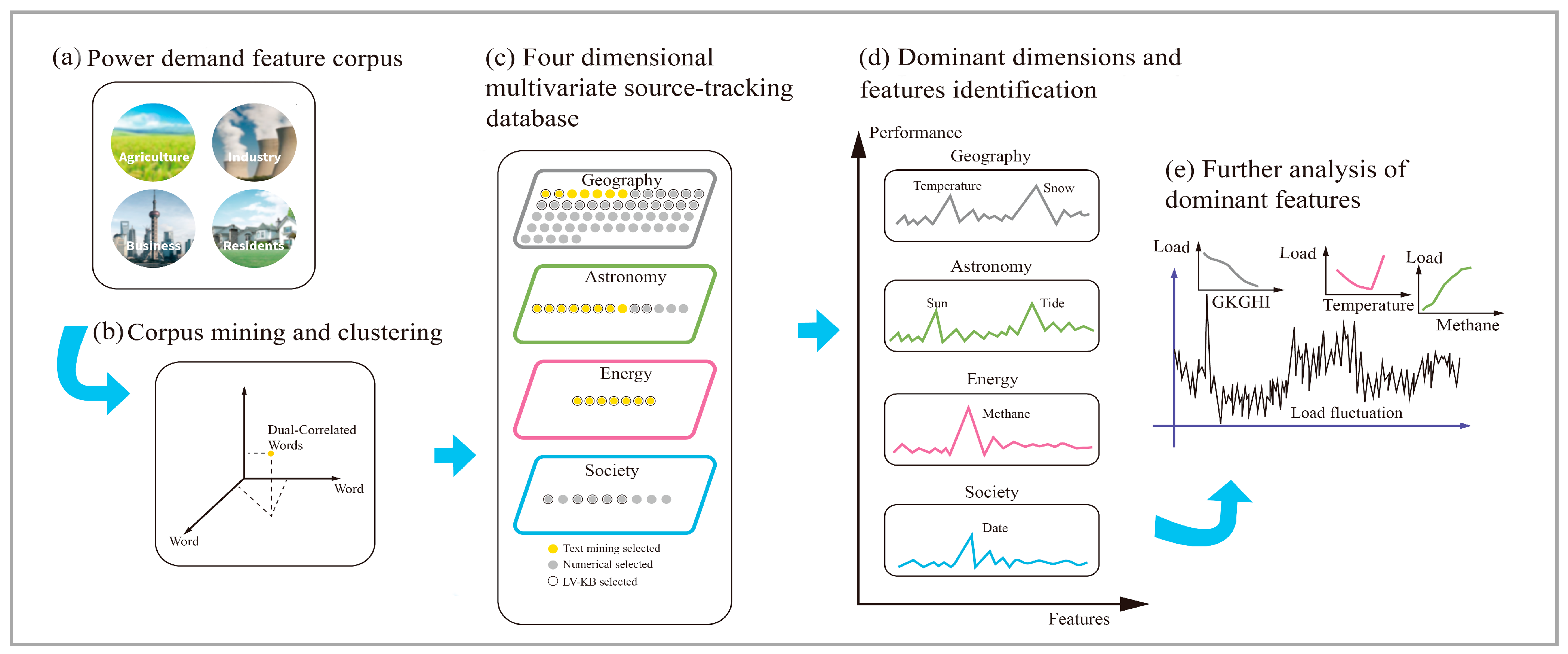
2. Discovery of Candidate Feature Set

2.1. Construction of Power Demand Feature Corpus

Electricity users are typically divided into four categories: agriculture, industry, business, and residential. To comprehensively gather knowledge on the diverse features affecting power consumption changes, this study employs these four categories of electricity users as an initial clue. We crawled over a thousand textual reports on the four user groups from the U.S. Department of Energy website (https://www.energy.gov/) and the New South Wales government website (https://www.energy.nsw.gov.au/) and rapidly constructed a power demand feature corpus.

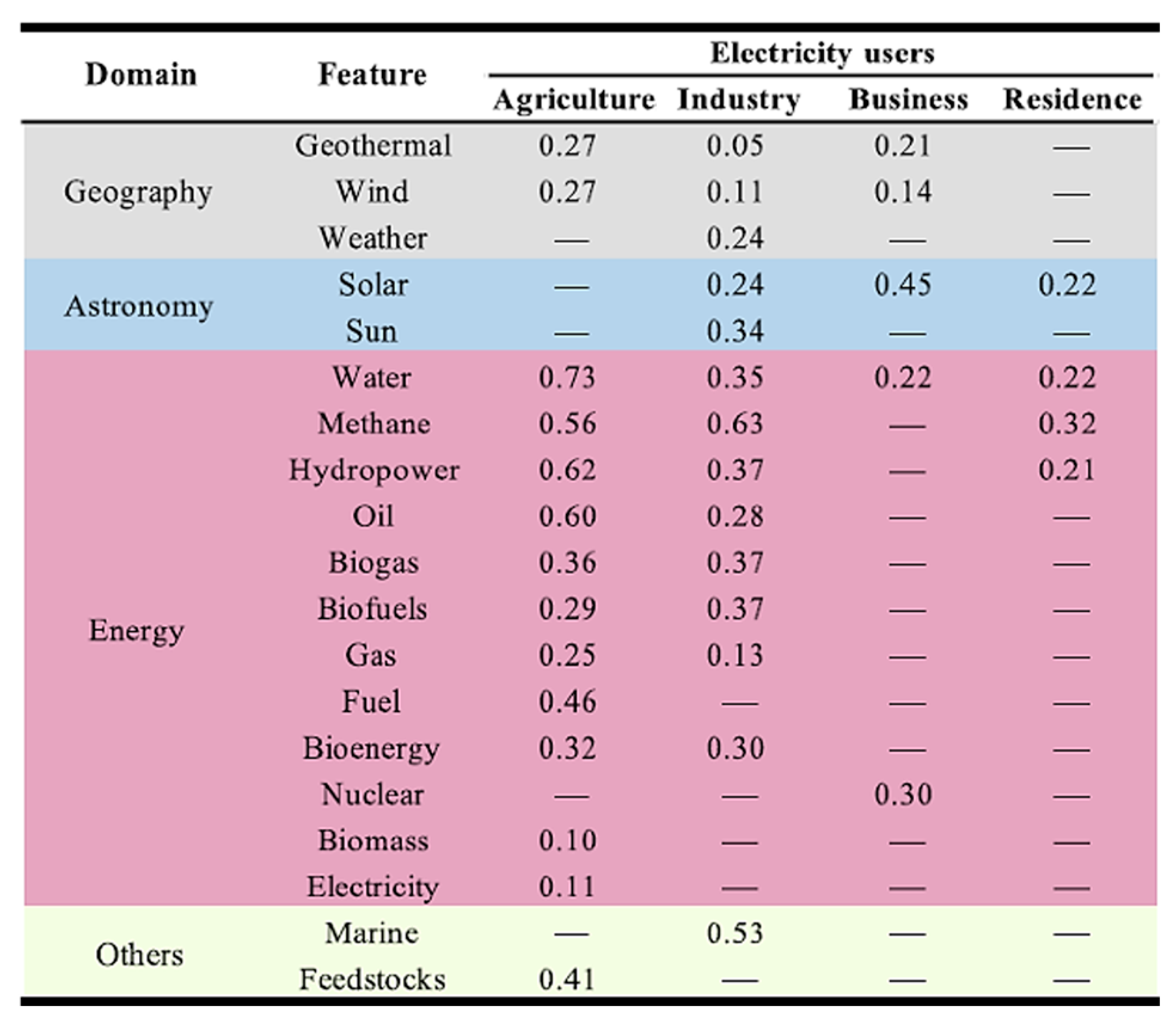
2.2. Text Mining on Power Demand Feature Corpus

With continued advancements in natural language processing [27,28], there is growing interest in leveraging corpus analysis [25,26] to uncover text similarities. The mutual information algorithm [29] has been proven to be effective in measuring similarities between discrete variables, and it can also be applied to continuous variables. As shown in Formula (1), mutual information I (X;Y) does not necessitate categorical ordering. It is derived from the joint probability distribution p(x,y) of random variables X and Y, along with their marginal probability distributions p(x) and p(y).
I X ; Y = x X y Y p x , y log p x , y p x p y
Experiments have shown that the algorithms that focus solely on text similarity fail to yield ideal results in the exploration of the SPDF-related features. This is due to the low independence among many similarity-matching words (e.g., (load, power)), which negatively impacts the results. Consequently, we need an algorithm that examines text similarities, eliminates words with low independence, and increases the weight of valid words like load and weather. However, there are still a few ideal algorithms to integrate words’ correlation and independence, which could keep the similarity between words while removing the low independent elements [30,31].
In this study, we propose the dual-correlated words (DCW) algorithm to identify words (i.e., candidate correlation features) that affect power demand fluctuation in the power demand feature corpus. The process of text mining on the power demand feature corpus is as follows.
Firstly, we use the DCW algorithm to assess the correlation between two words by considering both their similarity and independence, as shown in Formulas (2) and (3). The similarity between words in a corpus is represented by the cosine value of the angle between word vectors, while the independence between words is quantified by the point-wise mutual information (PMI) between texts. Based on mutual information, PMI identifies the co-occurrence of words from the perspective of statistics, analyzing whether there is semantic correlation or thematic correlation between words. Using the DCW algorithm, we set word1 as “load” and word2 as each successive word after traversing through the corpus.
D C W = P M I w o r d 1 ,   w o r d 2 c o s i n e w o r d 1 ,   w o r d 2
P M I w o r d 1 ,   w o r d 2 = log P w o r d 1 ,   w o r d 2 P w o r d 1 P w o r d 2
Then, assuming that we do not have any prior knowledge of the subject, we use TKNFD to process and classify the features we find. We implement the unsupervised k-means clustering algorithm with the word vector model built in the previous step to classify the discovered features, as shown below.
a k = i = 1 n z i k x i j i = 1 n z i k
z i k = 1 , i f x i a k 2 = min x i a k 2 0 , o t h e r w i s e
where X = x1, …, xn is the dataset in a D-dimensional Euclidean space Rd and A = a1, …, ac is the set of c cluster centers. Let z = [zik]n×c, where zik is a binary variable indicating if the data point xi belongs to the kth cluster, k = 1, …, c.
Finally, the found features are classified into approximately three dimensions using the k-means neighbor clustering algorithm [32,33], as shown in Figure 2. In addition to the dimensions that have been fully studied, such as geography and astronomy, a new classification has emerged, which mainly includes influencing factors such as biological gases and fossil fuels. We call this category the integrated energy dimension, a crucial impact dimension that previous studies have overlooked. The DCW score between the word ‘load’ and a correlated word is shown in this figure. The mark “—” represents that the DCW value of a word and the word ‘load’ is not higher than the set threshold (0.1).
Based on the DCW algorithm, the text mining result on the power load feature corpus is shown in Figure 2. This figure reveals that in the reports on the U.S. Department of Energy website [34,35], the influencing factors of power demand change mainly involve the domain features of three dimensions: geography, astronomy, and integrated energy. In the geographical dimension, weather and wind-related features influence power demand in agriculture, industry, and the economy. In the astronomical dimension, the main features related to the sun significantly affect industrial power consumption. In the integrated energy dimension, clean energy and fossil energy are highly weighted.

2.3. Creation of Candidate Feature-Type Set

We obtain three main dimensions from the power demand feature corpus through previous research. Inspired by the above feature corpus, along with the research work of our team in numerical feature extraction [6], we extend the domain features from three dimensions to four dimensions: geography, astronomy, integrated energy, and society. Each dimension consists of multivariate domain feature types. The geographical dimension includes weather, temperature, air pressure, humidity, etc. The astronomical dimension includes sunshine duration, civil dawn duration, lunar phase, tide, solar radiation, sunrise time, etc. The integrated energy dimension includes methane price, propane price, etc. The social dimension includes holidays, events, week types, etc. The four-dimensional multivariate feature-types and historical power demand feature-type constitute a candidate feature-type set, as shown in Formula (6).
X = [ G 1 ,   ,   G i ;   A 1 ,   ,   A j ;   I 1 ,   ,   I k ;   S 1 ,   ,   S l ;   L 1 ,   ,   L m ]
G, A, I, S, and L, respectively, represent domain feature dimensions of geography, astronomy, integrated energy, society, and historical power demand, and i, j, k, l, and m represent the number of domain feature types in each feature dimension.
With the candidate feature type set under the accumulation and inspiration of text modal knowledge, the dominant dimensions and their outperformed features can be revealed in subsequent studies.

3. Identification of Dominant Dimensions and Features

Having obtained the candidate feature-type set through the accumulation and inspiration of textual knowledge, the question arises as to which of the four candidate dimensions has the most significant impact on power demand, apart from the historical demand load dimension. Likewise, it is important to identify the features that critically affect SPDF accuracy. To answer these questions, numerical feature databases are constructed, and a two-stage quantitative feature identification strategy, independent of forecasting models, is employed to analyze the databases from the dominant dimension to the feature level.

3.1. Feature Database Construction

Guided by the discovered candidate feature-type set, we then attempted to collect numerical data of these different features to construct a four-dimensional multivariate source-tracking database (4DM-STD), which is a numerical modality feature database. However, collecting such feature data, involving multiple fields of astronomy, geography, energy, and society, can be challenging, as they are not always readily available or accessible. We put significant efforts into collecting them worldwide and eventually succeeded in establishing a 4DM-STD in Maine and Texas, USA, and NSW, Australia, respectively.
Maine’s power demand data are downloaded from the ISO-New England website (https://www.iso-ne.com/). Texas load data are collected from The Power Reliability Council of Texas (http://www.ercot.com/) and the load data type is daily peak load. Geography data are collected from U.S. Data.GOV (https://www.data.gov/), Natural Earth Data (https://naturalearthdata.com/), and United States Geological Survey (http://usgs.gov/). Astronomy data are collected from U.S. NOAA (http://gis.ncdc.noaa.gov/) and NASA’s Global Change Master Directory (http://gcmd.earthdata.nasa.gov/). Integrated energy data are collected from the U.S. National Renewable Energy Laboratory (https://www.nrel.gov/research/data-tools.html, accessed on 24 May 2025), U.S. Energy Information Administration (https://www.eia.gov/), MarketInsider (https://markets.businessinsider.com/), Maine Government (https://maine.gov), and U.S. DR Power (https://www.epa.gov/egrid). The NSW data are from the Australian Energy Market Operator (https://www.aemo.com.au/). Among them, the Texas natural gas price sold to electric power consumers (dollars per thousand cubic feet) and coal price (delivered to electric power stations) are released on a monthly basis. Bayesian estimation is characterized by its compatibility with prior distribution assumptions, adaptability to random missing data mechanisms, and capabilities in multiple imputation and propagation of uncertainty, effectively preserving temporal trends and quantifying parameter errors. Mean imputation neglects the dynamic characteristics of data distribution and underestimates variance. In KNN imputation, “nearest neighbors” may deviate from the global distribution, leading to imputed values that distort long-term trends while also being sensitive to the choice of K-value. Regression imputation, though capable of modeling linear relationships, relies on single imputation and ignores uncertainty in regression coefficients. Similarly, random forest imputation, as a single-value approach, lacks explicit modeling capability for parameter uncertainty. In this study, we consider the natural gas and coal price per day to be linearly distributed, and the missing values are random. Therefore, we subject the dataset to multiple imputations based on Bayesian estimation. We construct a 4DM-STD on Maine containing 92 candidate features from 2003 to 2017, a 4DM-STD on Texas containing 58 candidate features from 2002 to 2019, and a 4DM-STD on NSW containing 88 features spanning 1 January 2009, solstice 6 January 2010, and the load data type is a half-hour load. Here, we take Maine as the main task, Texas, and NSW as cross-sectional comparison to build our following experiments.

3.2. Dominant Dimension Identification

We adopt one of the model-independent SHAP explainer [36] to identify the dominant dimensions that impact demand forecasting. As shown in Figure 3, the integrated energy dimension has the most significant impact on demand forecasting, with a mainly negative correlation, which indicates that power demand is in some competition with other integrated energy features. The geographical and astronomical dimensions have a secondary impact. The social dimension has the weakest impact among the four dimensions.

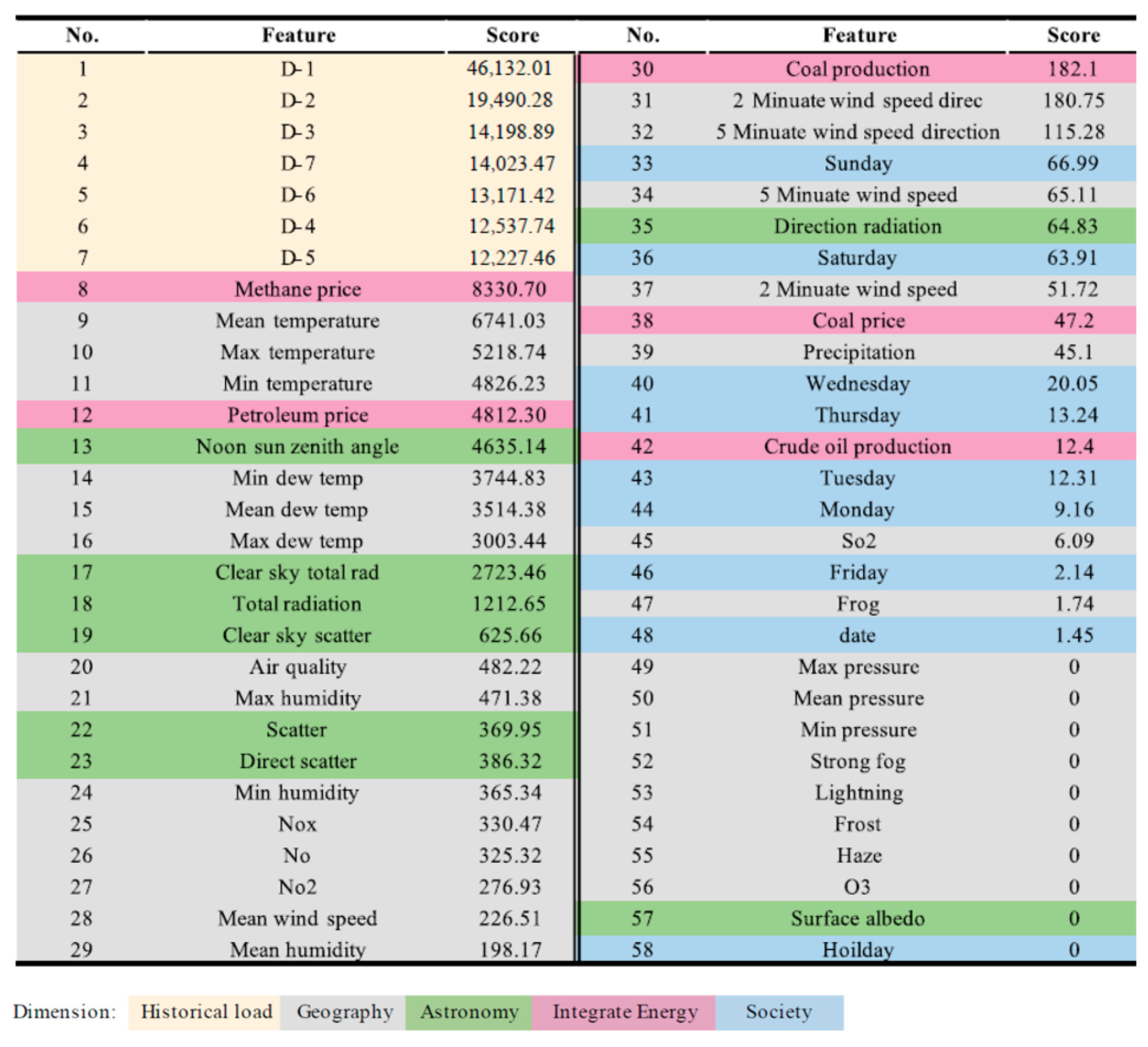
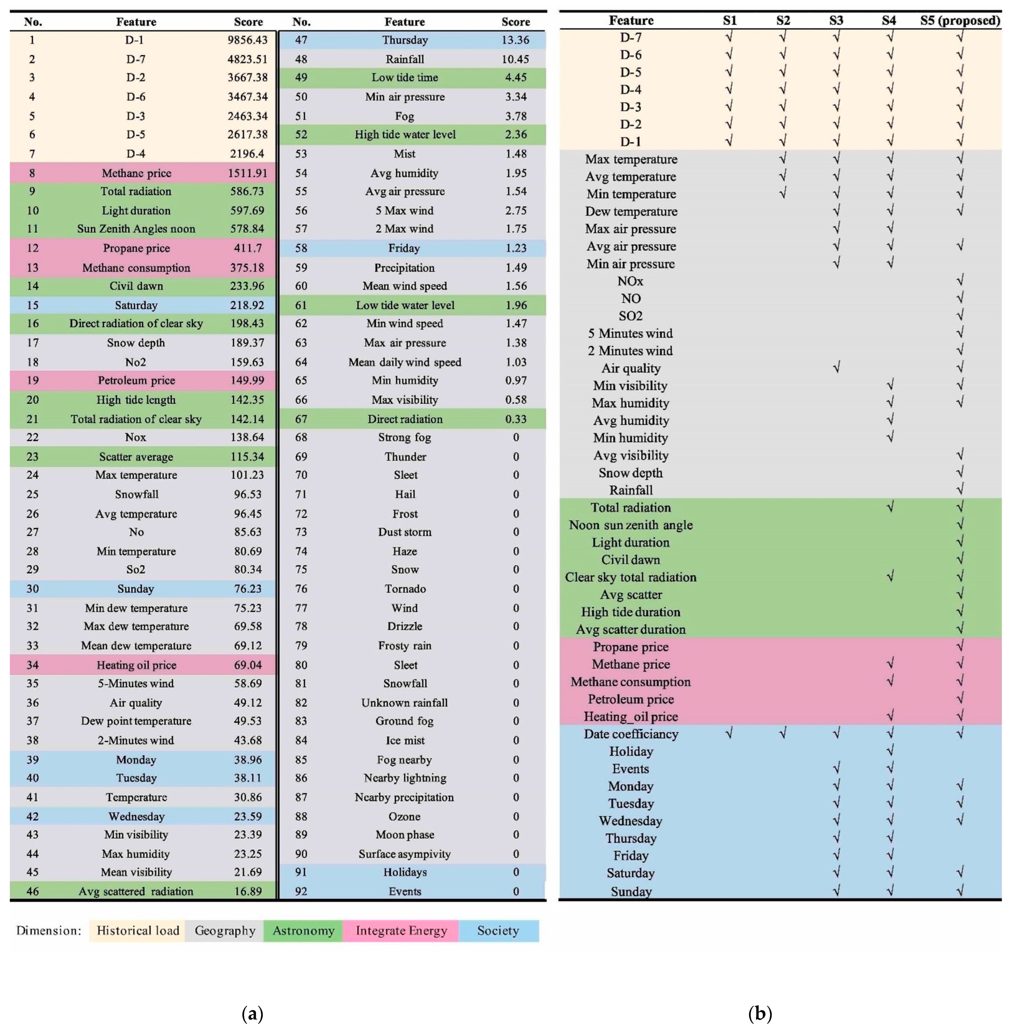
3.3. Feature Identification

LV-KB, a numerical feature filter algorithm, is chosen for dominant feature identification on 4DM-STD. LV-KB is a combination of Variance Thresholding and Select-K-Best. Variance Thresholding is a fast and lightweight way to eliminate the low variance features that do not express valid information. Using the Variance Threshold as the first feature filter can effectively improve the validity of the dataset and the computational efficiency of the model. According to the research experience of our team, the threshold of variance is set as 0.88. The Select-K-Best method, which is a univariate regression function, is used for further feature filtering. Assuming that the sample number of candidate features is n, the regression function first calculates the correlation coefficient ri between each feature xi,j and the label (i.e., power demand load) yj, as shown in Formula (7). Then, the feature score fi of the i-th feature can be calculated using Formula (8).
r i = j = 1 n X i j X - i y j y ¯ j = 1 n X i j X - i 2 j = 1 n y j y ¯ 2
f i = r i 2 1 r i 2 n 2
where X i j is the value of the i -th feature for the j -th sample, X - i is the mean of the i -th feature, y j is the value of the label variable for the j -th sample, y ¯ is the mean of the label variables, n is the number of samples, ri is the correlation coefficient between each feature and the label, and f i is the score of the i -th feature.
Feature filtering is then carried out according to the ranking of scores. Multiple experimental data from Maine show that when the threshold is set to 10, this filter can effectively reject invalid features and retain critical features. Dominant features are selected, as shown in Figure 4a. In total, 48 features are identified in Maine, in which 5 features belong to the integrated energy dimension, 28 to the geographic dimension, 9 to the astronomical dimension, and 6 to the social dimension. In the integrated energy and social dimensions, methane price and Saturday get the highest score, respectively, indicating that methane price and Saturday are the dominant features in the two dimensions, respectively. In astronomical and geographical dimensions, sun-related features and temperature have higher scores than other features, implying that sun-related features and temperature play essential roles in the two dimensions, respectively. In addition, except for the historical load dimension, the features of the integrated energy dimension rank the highest and those of the social dimension rank the lowest. This result is consistent with the conclusion in Section 3.2 that the integrated energy dimension has the most significant impact while the social dimension has the weakest impact on demand forecasting among the four dimensions.
Experimental data on Texas and NSW (see Figure A1 in Appendix A and Figure A3 in Appendix B) have shown that TKNFD can effectively reject invalid features and identify key features. In Texas, 58 features are identified, with methane price and Sunday receiving the highest scores in the integrated energy and social dimensions, respectively. Sun-related features and temperatures score higher than other features in the astronomical and geographic dimensions, respectively. The integrated energy dimension ranks the highest, while the social dimension ranks the lowest. In NSW, 88 features are identified, with methane price and time coefficient receiving the highest scores in the integrated energy and social dimensions, respectively. Sun-related features and temperatures play a vital role in the astronomical and geographic dimensions, respectively. Methane price is identified as the dominant feature in the integrated energy system, affecting load forecasting in that dimension. These results are consistent with the conclusion that temperature-dependent features dominate in the geographic dimension and solar-related features dominate in the astronomical dimension.

4. Forecasting Experiments and Performance Comparison of Proposed Features

4.1. Forecasting Experiments Overview

In order to investigate the effectiveness and generalization of the proposed features found by TKNFD, this paper selects three regions that differ significantly in geographical location, climate, population, and energy structure to establish a forecasting experiment. Maine is located in the northeastern U.S. (Northern Hemisphere), with cold winters, a relatively small population, and a strong reliance on renewable energy. Texas is in the southern U.S. (Northern Hemisphere), known for its hot dry weather, large population, and substantial reliance on fossil fuel-based power generation. New South Wales (NSW) lies on Australia’s east coast (Southern Hemisphere), featuring a diverse climate, a large population and a strong reliance on renewable energy. The forecasting experiment datasets are the 4DM-STDs of Marine, Texas, and NSW constructed in Section 3.1. In the case of Maine, the dataset from 2003 to 2014 is taken as the training set and the dataset from 2015 to 2017 as the test set. In the case of Texas, the daily peak load from 2002 to 2015 in the Power Reliability Council region is taken as the training set, and from 2016 to 2019 as the testing set. In the case of NSW, the data spans from 1 January 2009 to 6 January 2010, where one-tenth of the NSW dataset time windows are randomly drawn as the test set in order.
Three classical machine learning algorithms (support vector regression (SVR), gradient boosting regression trees (GBRT), and Transformer [37]) are built as the forecasting models. Besides, the transformer model we constructed contains 52 layers in total, including convolutional layers, dense layers, extract patch layers, attention layers, LSTM layers, and transpose layers. We select mean absolute percentage error (MAPE) for performance evaluation, as shown below, where y ^ t represents the forecasted power demand load value, y t represents the actual load value, and n is the number of load points.
M A P E = 1 n t = 1 n y ^ t y t y t × 100 %

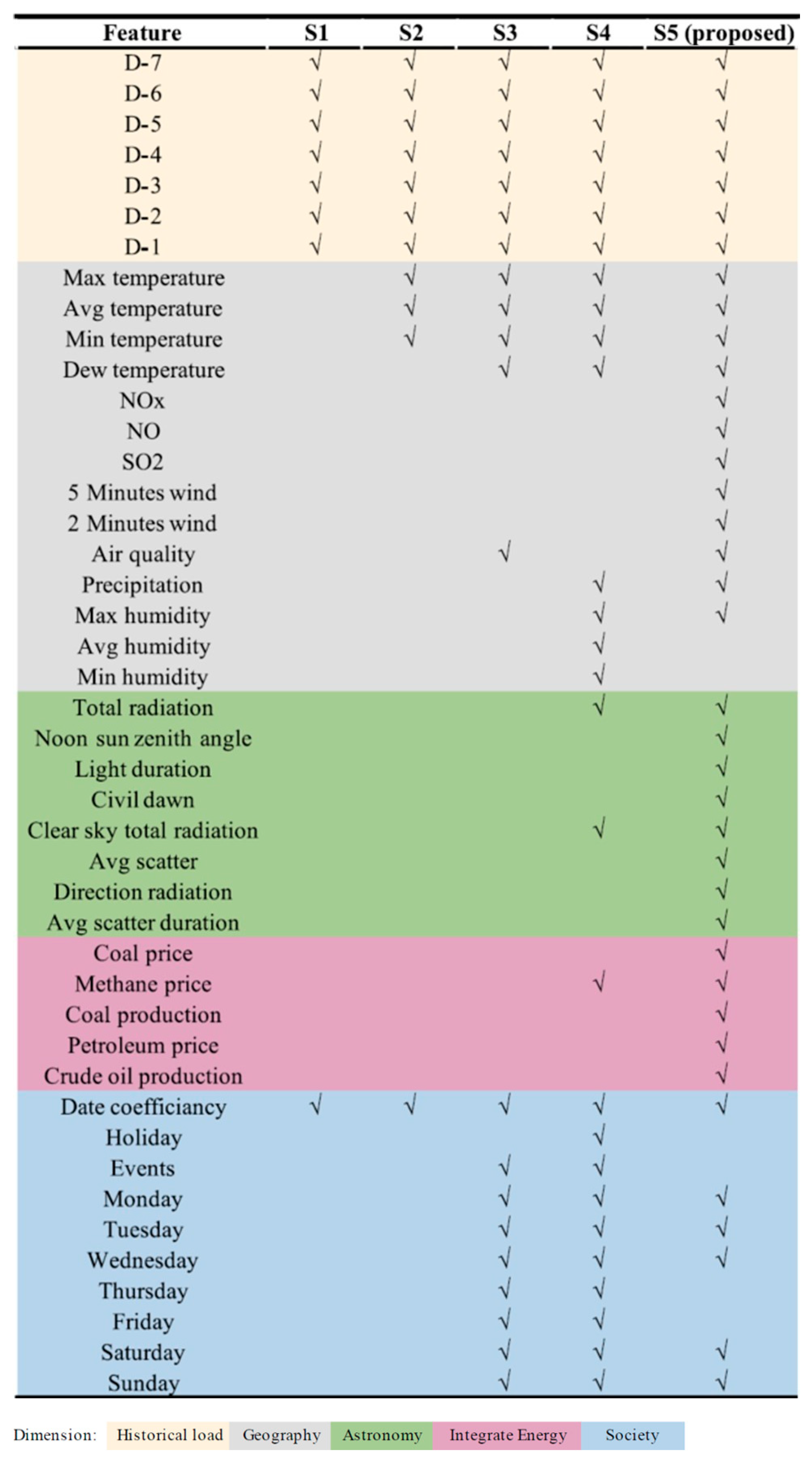
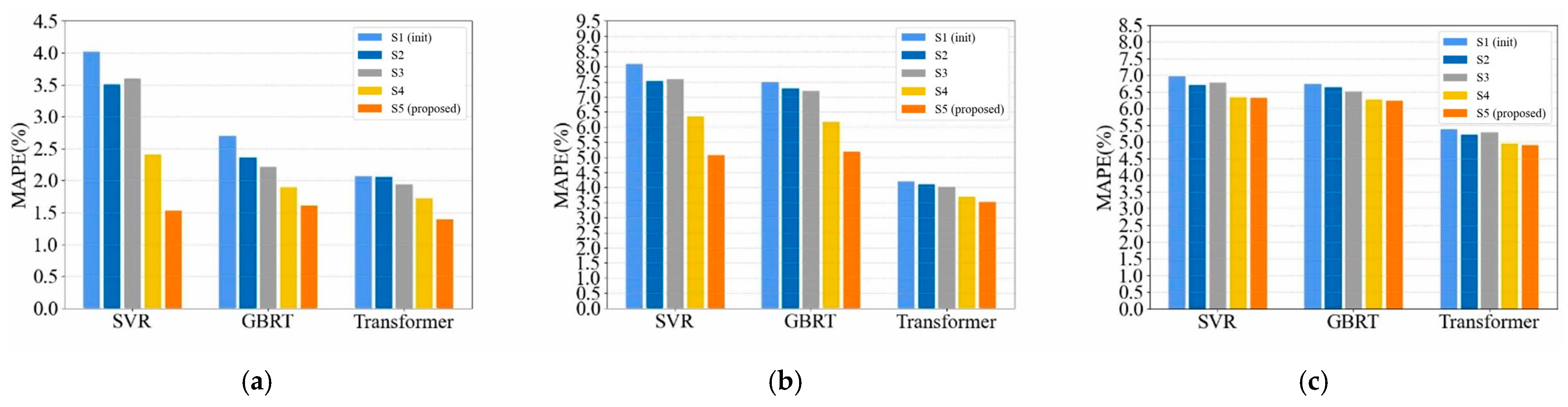
4.2. Comparison with the SoTA Feature Schemes

Based on state-of-the-art (SoTA) research, we design five feature schemes for comparative forecasting experiments in three regions. Here, we take Maine as an example, as shown in Figure 4b. Scheme 1 (S1), the baseline scheme, includes only the date coefficient and the history peak load. Scheme 2 (S2) adds 3 temperature-related features proposed by [38] on the basis of S1. Scheme 3 (S3), which is the Smart Grid Smart City dataset proposed by [39] on the basis of S2, filters nine social features in the proposed feature database. Scheme 4 (S4) adds three new energy features [16] based on S3; Scheme 5 (S5) is the features scheme identified by TKNFD, which is shown in Figure 4a. Figure 4b illustrates the designed feature schemes, where “✔” represents the feature that is included in this scheme.
Figure 5 presents the comparison results of forecasting accuracy between the feature scheme identified by our proposed TKNFD (i.e., S5) and the SoTA feature schemes (i.e., S1–S4). The comparative experimental results of Maine are shown in Figure 5a. As shown in Figure 5a, S1 has the poorest forecasting performance, S2 and S3 are comparable, and the forecasting accuracy of S5 is the highest. S1 contains only seven historical load features and date coefficients, while numerous studies have demonstrated that temperature is a critical factor affecting load changes. Compared to S1, S2 adds temperature features, resulting in a marked improvement in forecasting accuracy, highlighting the correlation between temperature and load fluctuation. S3 has nine more features than S2, including holidays, events, and week types. As discussed in Section 3, the social dimension has limited impact on SPDF. Therefore, the accuracy improvement brought about by S3 is less effective. Compared to S3, S4 adds some integrated energy features and astronomy features, leading to a distinct improvement in forecasting accuracy. S5 comprehensively covers the four dimensions of geography, society, integrated energy, and astronomy, in addition to historical loads. S5 also includes more features in different dimensions, particularly astronomical and integrated energy features. Clearly, S5, the features discovered by TKNFD, demonstrates the best forecasting accuracy among all feature schemes across all forecasting models. The MAPE of S5 is 16.84% to 36.37% lower than that of S4, and the MAPE of S5 is less than 1.62% for all three forecasting models.
The comparative experimental results of Texas and NSW are shown in Figure 5b,c, respectively. As shown in Figure 5b, after applying S4 with the main geographical dimensions and integrated energy system dimensions and the proposed TKNFD, the performance of power demand forecasting in the Texas scenario was significantly improved. Compared to the initial dataset, the performance of S5 in Texas was 16.08–37.31%. Texas’s 4TM-STD performed 3.55% MAPE on the Transformer model. As shown in Figure 5c, after applying S4 with main geographical dimensions and integrated energy system dimensions and the proposed TKNFD, the performance of power demand prediction in NSW scenarios significantly improved. Compared to the initial data set, the performance of S5 on NSW increased by 11.50%. NSW’s 4TM-STD performed 4.92% MAPE on the Transformer model.

4.3. Summary

The above forecasting experiments, utilizing five classical and advanced forecasting models across three distinct regions, demonstrate that the forecasting accuracy achieved with TKNFD-discovered features consistently surpasses that of SOTA feature schemes by up to 36.37% MAPE. In total, 43–48 features were discovered by TKNFD. Moreover, the TKNFD-identified feature scheme combined with simple machine learning forecasting algorithms can achieve high accuracy. This indicates that TKNFD can avoid the uninterpretability problem of complex models and effectively captures many source factors related to load fluctuations by adding the astronomical dimension and the energy dimension to the traditional geographical and social dimensions. In addition, while retaining the differentiation, the common points of different representative electricity consumption areas are found. Each dimension contains more diversified candidate features. Therefore, the candidate feature set built based on the 4DM-STD has effectively covered the dominant features of SPDF and can provide comprehensive and robust data support for various forecasting algorithms. In summary, these comparative experimental results verify that TKNFD is capable of discovering features systematically and comprehensively.

5. Further Analysis of Proposed Features

Due to space constraints and the richness of the Maine data, we choose Maine as the primary case study, along with Texas and New South Wales as cross-sectional comparative case studies (see Appendix A and Appendix B).

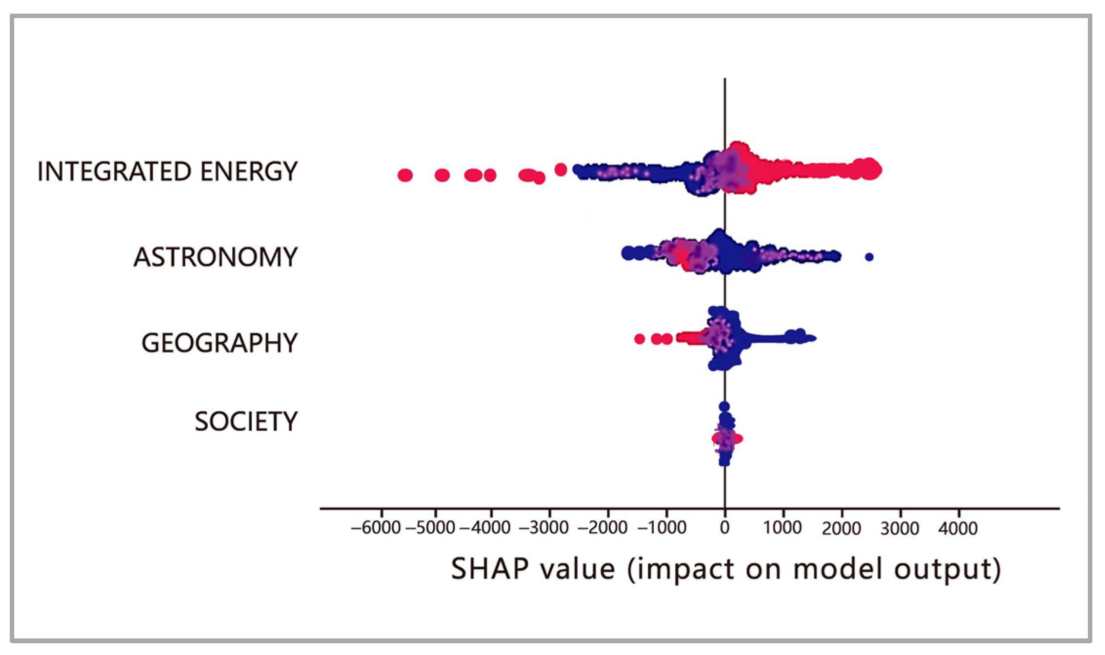
5.1. Sensitivity Analysis of Feature Contributions

This section analyzes Maine as a case study. Sensitivity analysis involves studying the uncertainty in the output of a model and further determining the source of uncertainty to study the degree of output change caused by the change in input parameters. Sobol sensitivity analysis, a variance-based sensitivity analysis method, quantifies the uncertainty of the input and output in the form of a probability distribution and decomposes the output variance into parts that can be attributed to the input variables and combinations of variables. Any model may be viewed as a function Y = f (x).
Y = f 0 + i = 1 d f i ( X i ) + i < j d f i j X i , X j + + f 1 , , d ( X 1 , , X d )
where f0 is a constant and fi is a function of Xi, fij a function of Xi and Xj, etc.
To ensure that the feature data dimension does not affect the results of the sensitivity analysis, we normalize all the feature data separately and combine them for a sensitivity analysis by dimension. The Sobol method is selected to calculate the parameter sensitivity of the MLP regression model, which performs well in the above experiments. Assuming that the parameters are uniformly distributed, the Monte Carlo sample number n is set to 1000, and four parameters are analyzed. The results of the Sobol sensitivity analysis are shown in Table 1.
Here, S1 represents the first-order indices; S2 represents the second-order indices, which reveal the intensity of the interaction between the two parameters; ST represents the total-effect index; and S1conf, S2conf, and STconf represent the corresponding confidence levels, respectively.
The table shows that SPDF is more sensitive to changes in integrated energy parameters and less sensitive to social parameters. The second-order indices (S2) reveal the intensity of the interaction between two parameters. In this case, the S2 analysis shows that the intersection between different dimensions is not vital, and there is no apparent correlation. The Sobol sensitivity analysis confirms the different contributions of the four dimensions identified by SHAP analysis in Section 3.2.

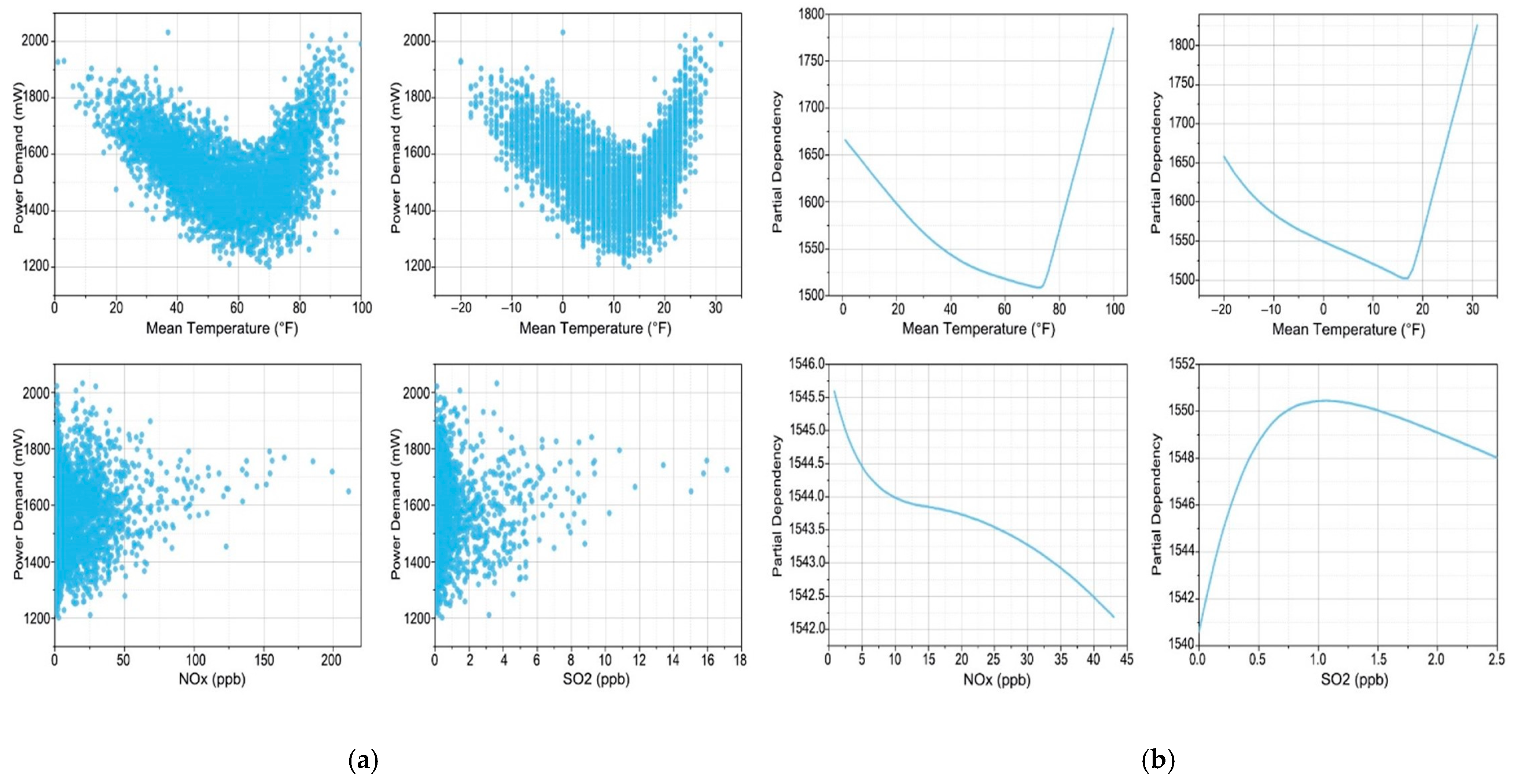
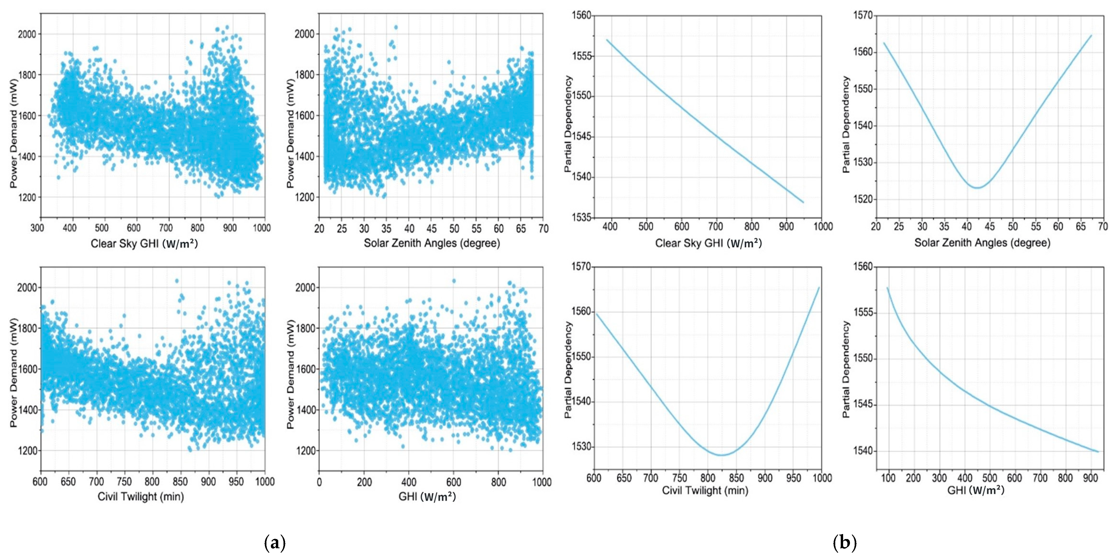
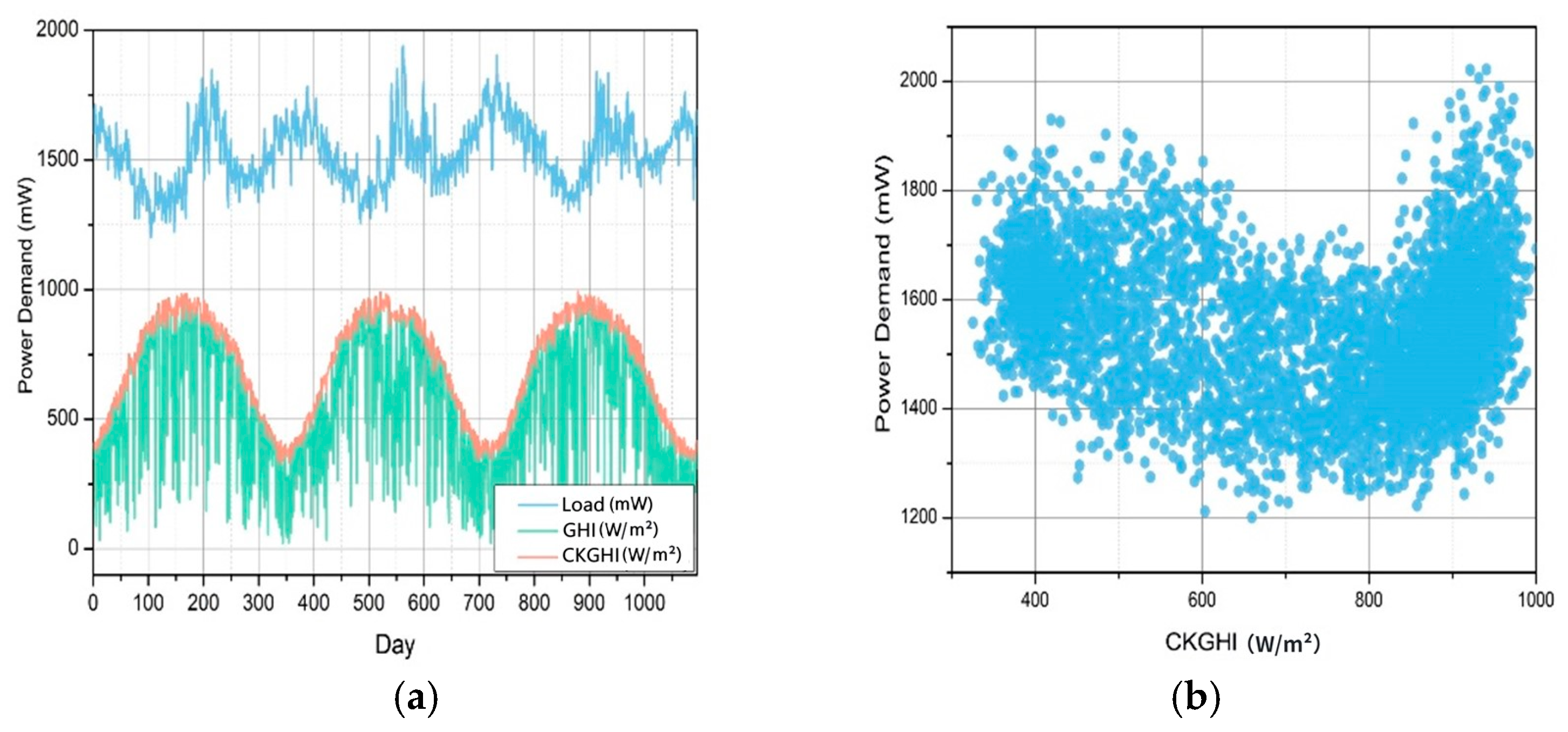
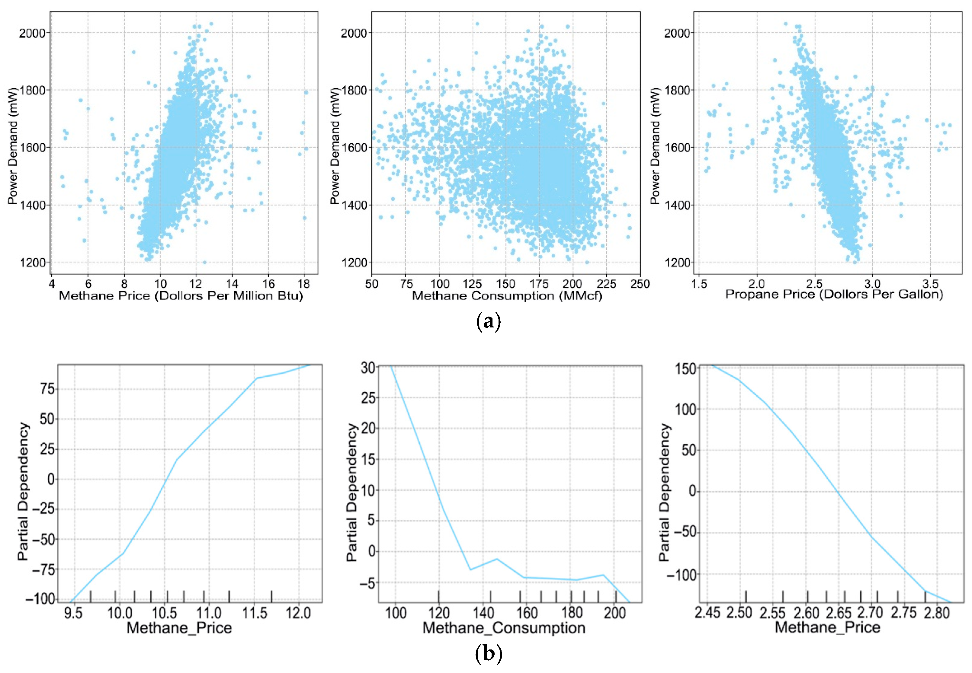
5.2. Dependency Relationship Analysis

To further investigate the dependency relationship between features and demand load changes and how dominant features affect demand forecast results, this paper employs a partial dependence plot and beeswarm plot to explore the relationships between load fluctuation and dominant factors in the case of Maine. For a trained model, a partial dependence plot can depict the response of the model’s forecasting results to a single feature change. The partial dependence function is defined as follows:
f ^ x j = 1 n i = 1 n f ^ ( x j , x j , i )
where f ^ represents the trained model, n represents the number of samples in the training set, xj represents other features except for xj, and the partial dependence of xj is defined as the mean value of forecasted values obtained by f ^ force when xj is fixed, and xj changes within its range.
We focus on the maximum and mean temperature features to examine the relationship between temperature and demand load, along with NOx and SO2, to investigate the relationship between atmospheric indices and demand load. As shown in Figure 6a, the fluctuation between the two temperature features and the demand load presents a V-shape. This phenomenon is also evident in Figure 6b, where the change in temperature and load exhibits an inverse linear relationship below and above a certain temperature threshold, referred to as the temperature equilibrium point [40]. The equilibrium point is approximately 70 °F for the maximum temperature and 15 °F for the mean temperature. When the temperature exceeds or falls below this threshold, the use of air conditioning or heating equipment increases power demand. In the partial dependence plot for NOx, the forecasted load value and NOx content exhibit a negative correlation. For SO2, the forecasted load value increases when the SO2 content is between 0 and 1 ppb. However, when the content exceeds 1 ppb, the demand load forecasting value decreases gradually.
As shown in Figure 7b, the solar zenith angle (SZA) and civil twilight duration also exhibit a V-shaped relationship with the forecasted load value, indicating the presence of equilibrium points where the load is minimized. The SZA equilibrium point is approximately 42°, and the civil dawn length equilibrium point is about 820 min. When latitude is determined, the position between the Earth and the Sun is reflected by the SZA at noon and the duration of civil dawn, which exhibit a significant annual periodic pattern. Intermediate values correspond to spring or autumn, while higher or lower values correspond to summer or winter. As shown in Figure 7a,b, load fluctuations are negatively correlated with the global horizontal irradiance (GHI) in clear sky conditions.
As shown in Figure 8a, the daily peak load, GHI, and clear sky global horizontal irradiance (CKGHI) all exhibit annual periodic changes. However, the change period of GHI and CKGHI is twice as long as that of the daily peak load. The two peaks of the load correspond to the peak and trough of CKGHI but exhibit a phase difference, with the load lagging CKGHI by approximately 50 days. Figure 8b shows that CKGHI and the daily peak load exhibit a V-shaped relationship after a 50-day lag. Due to the large specific heat capacity of the ocean, the heat accumulation received by the Earth from the Sun is relative to solar radiation. The heat absorbed by the Earth reaches its maximum value 1–2 months after the maximum solar radiation. This heat accumulation drives changes in climate and weather, which influence load fluctuations. Consequently, load fluctuations exhibit a lagged response to changes in solar radiation.
Figure 9 illustrates the relationship between power demand and three energy factors: methane price, methane consumption, and propane price. The methane price exhibits a positive linear correlation with power demand, while methane consumption and propane price exhibit negative linear correlations with power demand. This relationship can be explained by the properties of these energy sources. Biogas, which is primarily represented by methane, forms a complementary relationship with power generation. Thus, an increase in methane prices leads to a corresponding increase in power consumption. On the other hand, propane, which is the primary energy source exported by the United States, competes with power generation for consumption. A rise in propane prices decreases export volume, promotes internal consumption, reduces power generation, and ultimately negatively affects power demand.
This study was carried out in Maine and Texas, U.S., and New South Wales, Australia. According to the data provided by Wind Company, the natural gas prices in the United States and Europe reached new record highs in 2020–2021. On 27 September 2021, U.S. NYMEX October natural gas futures rose by 11.01%, setting a new record since 2014. With the soaring price of natural gas, the power demand in both the United States and Europe follows an obvious increase. This phenomenon validates the conclusion revealed by TKNFD that methane price acts as a dominant feature of power demand and positively correlates with power demand, which also strongly indicates the applicability of TKNFD to different regions.

5.3. Lagging Effect Analysis

Our examination of time domain behavior shows that some features exhibit significant lagging effects on power demand. In terms of geographic dimensions, the daily average temperature remains stable with minimal fluctuations. However, the peak of the daily average temperature coincides with the peak of power demand and has a lagging effect on power demand of around 10 days. The peaks and valleys of the daily average dew point temperature also coincide with power demand and have a lagging effect on power demand of approximately 5–10 days. In terms of astronomical dimensions, sun-related features have a more significant lagging effect on power demand. These features are positively correlated with power demand as a whole and have a lagging effect on power demand of approximately 50 days. Features in the IES dimension are relatively stable. Among them, natural gas consumption shows a clear seasonal fluctuation trend and is negatively correlated with power demand, with a lagging effect of approximately 30 days. Correspondingly, natural gas prices fluctuate positively with power demand and have a 30-day lagging effect on power demand. On the other hand, propane prices fluctuate negatively with power demand and have a 30-day lagging effect on power demand.

6. Conclusions

In this study, we propose a novel feature discovery framework called TKNFD. Unlike traditional feature engineering and representation learning approaches, TKNFD establishes interactions between text modal data—a potentially valuable yet long-overlooked resource in the field of power demand forecasting—and numerical modal data. The essence of TKNFD lies in fully exploiting the dual relationships of synonymy and complementarity between text modal data and numerical modal data in terms of granularity, scope, and temporality. Through this approach, TKNFD discovers 4 domain dimensions, 58–92 candidate feature types, and 38–50 features, which are twice, 5–9 times, and 1.6–5 times as many as empirical feature engineering methods, respectively. Benchmark forecasting experiments utilizing five classical and advanced forecasting models across three regions demonstrate that the forecasting accuracy achieved with TKNFD-discovered features consistently surpasses that of state-of-the-art feature schemes by up to 36.37% MAPE in Maine, 20.09% MAPE in Texas, and 1.21% MAPE in NSW. These results confirm the systematic and comprehensive nature of TKNFD in feature discovery.
Notably, driven by multimodal interaction, TKNFD can discover previously unknown interpretable features without relying on prior empirical knowledge. Specifically, TKNFD reveals that while some previously unknown features exist in the empirically known geographic and social dimensions, many others—especially several dominant features—exist in the previously unknown integrated energy and astronomical dimensions. The contributions and explanations of each dimension and its features are summarized as follows. (1) Integrated Energy Dimension: This dimension demonstrates the most significant improvement in SPDF accuracy, with methane price identified as the dominant feature. A positive correlation exists between methane price and load demand, with a lag of approximately 30 days. (2) Astronomical Dimension: Sun-related features play an important role in this dimension, generally exhibiting a 50-day lag effect on power demand. The solar zenith angle, civil twilight duration, and lagged clear sky global horizontal irradiance display a V-shaped relationship with power demand, indicating the presence of balance points. Additionally, global horizontal irradiance is negatively correlated with power demand. (3) Geographical Dimension: Temperature is a key feature influencing load change, also demonstrating a V-shaped relationship with power demand. (4) Social Dimension: Among the four dimensions, the social dimension has the weakest impact. Saturday and Monday are more important than other features in this dimension. These findings enhance our understanding of the complex and nonlinear nature of power demand fluctuations during the ongoing low-carbon transition in power sectors and IES. By illuminating the contributions of various dimensions and features, this study provides valuable actionable insights for policymakers and planners aiming to foster collaboration and competition between the power sector and other energy sectors in developing a new IES with low-carbon objectives.
We have made much effort to construct three 4DM- STDs, encompassing four feature dimensions and 58–92 candidate features. While we qualitatively identified a substantial number of features within the candidate feature-type set, the current unavailability of numerical data for some features has limited their inclusion in the 4DM-STDs. Nevertheless, despite the imperfect completeness of 4DM-STDs, these databases can serve as public baseline resources for SPDF.
The time consumption of the TKNFD process includes two aspects: (1) the text mode processing stage, including automated crawlers, text mining DCW algorithm, and 4DM-STD construction, which takes approximately several hours to several days, depending on the existing data scale in the study area; and (2) the numerical mode processing stage, mainly including the SHAP + LV-KB algorithm, which takes a short time, from seconds to minutes. As for the industrial deployment of TKNFD, it is recommended to use API interfaces or automated crawler tools, which could significantly shorten the construction time of the 4DM-STD database. In terms of the forecasting application of TKNFD, we observed that the forecasting model Transformer achieves high accuracy on three datasets in our benchmark experiments. It is recommended to use hardware acceleration and parallel computing technology to further improve its real-time performance. In addition, incorporating advanced forecasting processes and models, such as [41,42], into the TKNFD framework represents a potential future research pathway for enhancing the forecasting accuracy of TKNFD application.
In conclusion, the proposed TKNFD is a framework in which the specific technologies employed at each stage are not restricted to those presented in this paper. Its core focuses on multimodal interaction for both systematic and experience-independent discovery of interpretable features. TKNFD is not confined to feature discovery for power demand forecasting in the power sector. It is applicable to feature discovery in various fields, such as energy systems and epidemic forecasting tasks, where underlying mechanisms remain unclear and public feature databases are unavailable.

Author Contributions

Conceptualization, M.J.; methodology, M.J. and Z.N.; experiment and software, Z.N. and P.Z.; writing—original draft preparation, Z.N. and P.Z.; writing—review and editing, M.J.; supervision, M.J. All authors have read and agreed to the published version of the manuscript.

Funding

This work was supported by the Natural Science Foundation of Changsha (Grant number kq2402084), the Natural Sciences Foundation of Hunan Province (Grant number 2025JJ50343), and the National Key Research and Development Program of China (Grant number 2023YFC3503404).

Data Availability Statement

The preprocessed data and code are available at https://github.com/zifanning/TKNFD (accessed on 20 March 2023), and proper citation of this data and code is required.

Conflicts of Interest

The authors declare no conflict of interest.

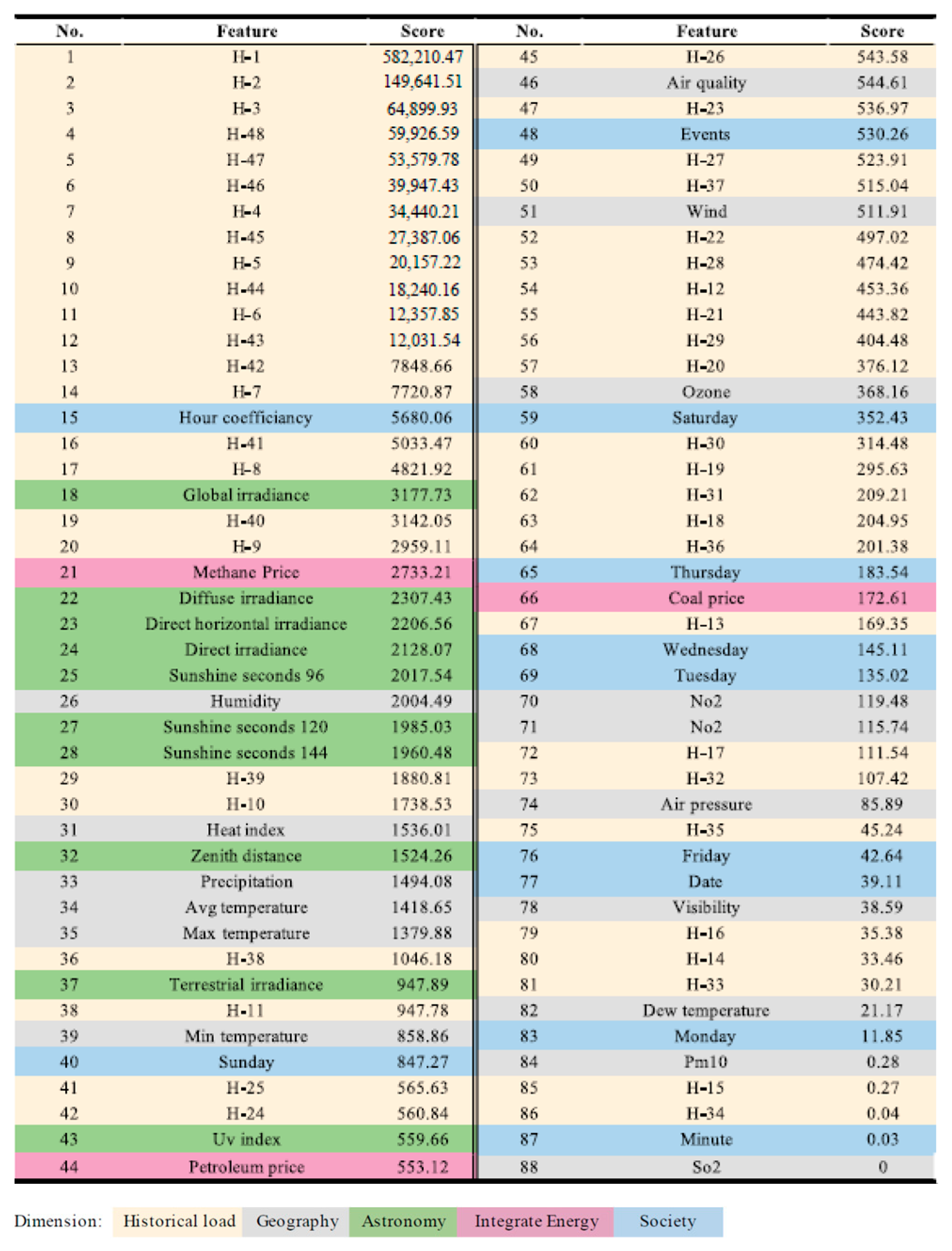
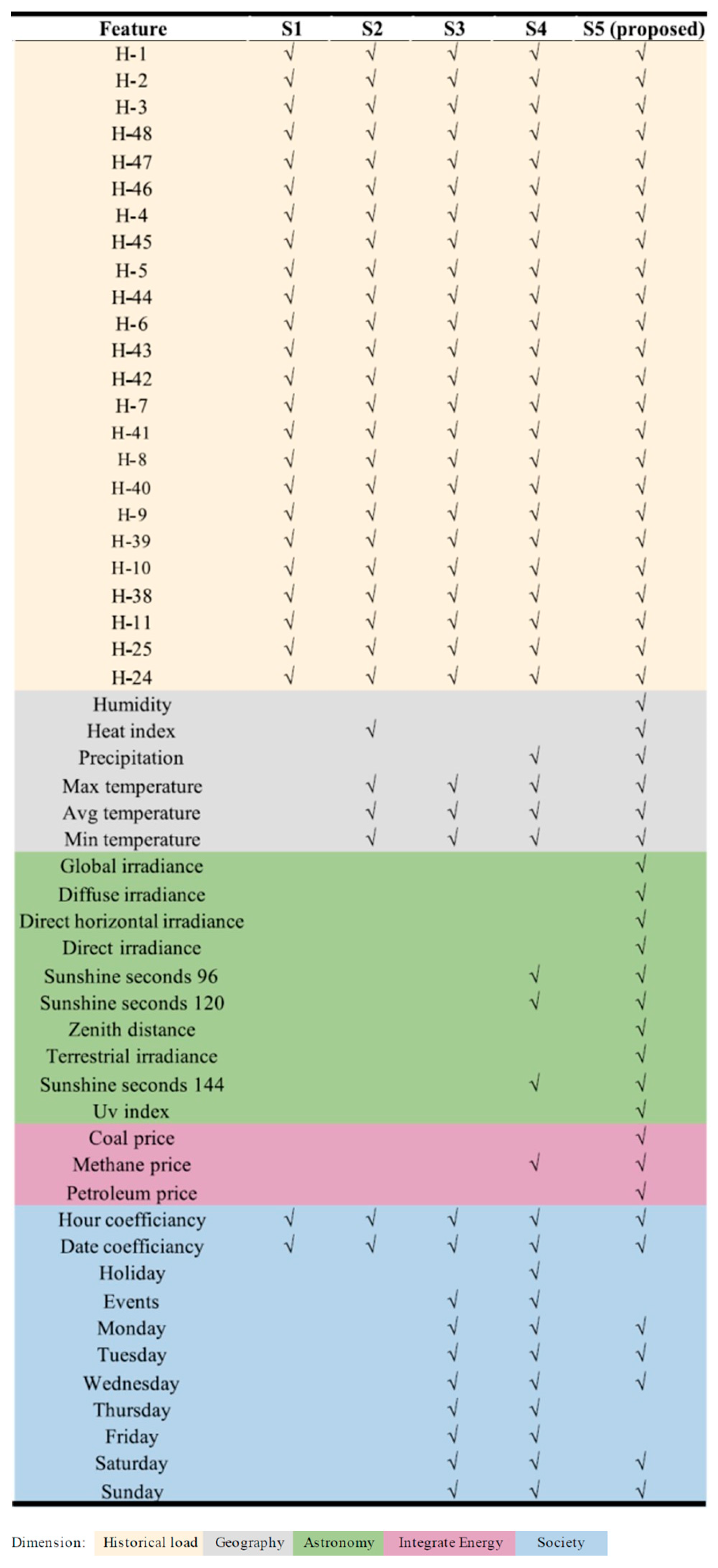
Appendix A. The Texas Case

The electricity consumption in Texas is influenced by various factors in the dimensions of geography, astronomy, society, and integrated energy, according to the TKNFD-discovered result. Geographical factors are among the most important, as Texas is a vast state with significant differences in electricity demand across different regions. Urban areas exhibit higher commercial and industrial electricity usage, while rural areas demonstrate greater residential electricity consumption. Astronomical factors also play a crucial role in affecting electricity consumption in Texas. The state’s diverse climate results in a surge in air conditioning and heating power usage during high temperatures in summer and low temperatures in winter. Social and economic development represents another critical factor influencing electricity consumption in Texas. As the second-largest state in the US with a large population, population growth and economic development bring increased power demand, especially in the industrial and commercial sectors. Additionally, the state’s population structure influences electricity consumption, with an increase in elderly and child populations leading to an increase in power usage in healthcare and education. The state’s energy structure and consumption patterns also affect electricity consumption in Texas. Texas is the largest wind and solar power generation state in the US, and its renewable energy production ranks first in the country. Wind and solar power generation in Texas are strongly affected by weather conditions, which have an impact on power load forecasting and usage. Fluctuations in natural gas and oil prices also affect power production costs and consumer prices.
Multiple experimental datasets from Texas demonstrate that when the threshold is set to 180, the filter can effectively eliminate invalid features and retain key features. The main features, as shown in Figure A1, include 58 features identified by Texas, comprising 5 in the integrated energy dimension, 29 in the geographical dimension, 8 in the astronomical dimension, and 9 in the social dimension. In the integrated energy and social dimensions, methane price and Sunday attained the highest scores, respectively, suggesting that methane price and Sunday are the dominant features of these two dimensions. Sun-related features and temperatures achieved higher scores than other features on astronomical and geographic dimensions, indicating that sun-related features and temperatures play a vital role in these two dimensions, respectively. Apart from the historical load dimension, the integrated energy dimension features ranked the highest, and the social dimension features ranked the lowest.
Texas’s forecasting scheme is primarily constructed from geographic and astronomical dimensions, as shown in Figure A2. Geographic dimensions comprise weather-related features, humidity-related features, wind-related features, and so on. The astronomical dimension is dominated by sun-related features, including clear sky total radiation, total radiation, noon sun zenith angle, etc. In the final scheme, the features of average humidity, minimum humidity, holidays in the social dimension, and major events in the geographical dimension were selected by the LV-KB scheme.
Figure A1. Dominant feature identification in Texas.
Energies 18 02907 g0a1
Figure A2. Feature schemes in Texas.
Energies 18 02907 g0a2

Appendix B. The NSW Case

New South Wales, located in southeastern Australia, has a population of over 8 million people. The state’s energy sector plays a vital role in its infrastructure, with city demand serving as a key indicator of economic activity and social development. The state’s diverse terrain influences power demand, with different regions exhibiting distinct weather patterns. Coastal areas may witness higher demand during the summer months due to air conditioning usage, while inland regions may see higher demand during winter months due to heating usage. NSW’s position in the Southern Hemisphere results in different daylight hours and seasonal changes compared to the Northern Hemisphere. NSW is a diverse and multicultural state with varied lifestyles and household structures that affect power demand. The state has a diverse mix of energy sources, including coal, natural gas, and renewable energy sources, such as wind and solar, which can influence power demand. During periods of high demand, the state may increasingly rely on coal-fired power plants to meet its power needs.
Multiple experimental datasets from Texas demonstrate that when the threshold is set to 550, the filter can effectively eliminate invalid features and retain key features. The main features, as shown in Figure A3, include 88 features identified by NSW, comprising 3 in the integrated energy dimension, 13 in the geographical dimension, 10 in the astronomical dimension, and 11 in the social dimension. In the integrated energy and social dimensions, methane price and time coefficient attained the highest scores, suggesting that methane price and time coefficient are the primary features of these two dimensions, respectively. Sun-related features and temperatures achieved higher scores than other features in the astronomical and geographic dimensions, indicating that sun-related features and temperatures play a crucial role in these two dimensions. This result is aligned with the conclusion in Section 3.2 that temperature-dependent features are dominant in the geographic dimension and that solar-related features dominate in the astronomical dimension. Methane price, as the dominant feature in an integrated energy system, significantly influences load forecasting in the dimension of an integrated energy system.
Figure A3. Dominant feature identification in NSW.
Energies 18 02907 g0a3
NSW’s forecasting scheme is primarily constructed from historical and astronomical dimensions, as shown in Figure A4. The astronomical dimension is mainly sun-related features, including clear sky total radiation, total radiation, noon solar zenith angle, ultraviolet index, etc. In the final scheme, social dimension features such as holidays, major events, Fridays, etc., were selected by the LV-KB scheme.
Figure A4. Feature schemes in NSW.
Energies 18 02907 g0a4

References

  1. Zhao, J.; Li, F.X.; Zhang, Q.W. Impacts of Renewable Energy Resources on the Weather Vulnerability of Power Systems. Nat. Energy 2024, 9, 1407–1414. [Google Scholar] [CrossRef]
  2. Saadaoui, A.; Ouassaid, M.; Maaroufi, M. Overview of Integration of Power Electronic Topologies and Advanced Control Techniques of Ultra-Fast EV Charging Stations in Standalone Microgrids. Energies 2023, 16, 1031. [Google Scholar] [CrossRef]
  3. Zhu, J.; Dong, H.; Zheng, W.; Li, S.; Huang, Y.; Xi, L. Review and Prospect of Data-Driven Techniques for Load Forecasting in Integrated Energy Systems. Appl. Energy 2022, 321, 119269. [Google Scholar] [CrossRef]
  4. Hafeez, G.; Khan, I.; Jan, S.; Shah, I.A.; Khan, F.A.; Derhab, A. A Novel Hybrid Load Forecasting Framework with Intelligent Feature Engineering and Optimization Algorithm in Smart Grid. Appl. Energy 2021, 299, 117178. [Google Scholar] [CrossRef]
  5. Bai, W.; Zhu, J.; Zhao, J.; Cai, W.; Li, K. An Unsupervised Multi-Dimensional Representation Learning Model for Short-Term Electrical Load Forecasting. Symmetry 2022, 14, 1999. [Google Scholar] [CrossRef]
  6. Zhou, M.; Jin, M. Holographic ensemble forecasting method for short-term power load. IEEE Trans. Smart Grid 2017, 10, 425–434. [Google Scholar] [CrossRef]
  7. Miraki, A.; Parviainen, P.; Arghandeh, R. Electricity demand forecasting at distribution and household levels using explainable causal graph neural network. Energy AI 2024, 16, 100368. [Google Scholar] [CrossRef]
  8. Abedinia, O.; Amjady, N.; Zareipour, H. A new feature selection technique for load and price forecast of electrical power systems. IEEE Trans. Power Syst. 2016, 32, 62–74. [Google Scholar] [CrossRef]
  9. Elahe, M.F.; Jin, M.; Zeng, P. Knowledge-based systematic feature extraction for identifying households with plug-in electric vehicles. IEEE Trans. Smart Grid 2022, 13, 2259–2268. [Google Scholar] [CrossRef]
  10. Xie, J.; Hong, T. Temperature scenario generation for probabilistic load forecasting. IEEE Trans. Smart Grid 2016, 9, 1680–1687. [Google Scholar] [CrossRef]
  11. Xie, J.; Chen, Y.; Hong, T.; Laing, T.D. Relative humidity for load forecasting models. IEEE Trans. Smart Grid 2016, 9, 191–198. [Google Scholar] [CrossRef]
  12. You, M.; Wang, Q.; Sun, H.; Castro, I.; Jiang, J. Digital twins based day-ahead integrated energy system scheduling under load and renewable energy uncertainties. Appl. Energy 2022, 305, 17899. [Google Scholar] [CrossRef]
  13. Son, H.; Kim, C. Short-term forecasting of electricity demand for the residential sector using weather and social variables. Resour. Conserv. Recycl. 2017, 123, 200–207. [Google Scholar] [CrossRef]
  14. Zeng, P.; Sheng, C.; Jin, M. A learning framework based on weighted knowledge transfer for holiday load forecasting. J. Mod. Power Syst. Clean Energy 2019, 7, 329–339. [Google Scholar] [CrossRef]
  15. Aguilar Madrid, E.; Antonio, N. Short-term electricity load forecasting with machine learning. Information 2021, 12, 50. [Google Scholar] [CrossRef]
  16. Zhu, R.; Guo, W.; Gong, X. Short-term load forecasting for CCHP systems considering the correlation between heating, gas and electrical loads based on deep learning. Energies 2019, 12, 3308. [Google Scholar] [CrossRef]
  17. Wang, S.; Wang, S.; Chen, H.; Gu, Q. Multi-energy load forecasting for regional integrated energy systems considering temporal dynamic and coupling characteristics. Energy 2020, 195, 116964. [Google Scholar] [CrossRef]
  18. Türkoğlu, A.S.; Erkmen, B.; Eren, Y.; Erdinç, O.; Küçükdemiral, İ. Integrated approaches in resilient hierarchical load forecasting via TCN and optimal valley filling based demand response application. Appl. Energy 2024, 360, 122722. [Google Scholar] [CrossRef]
  19. Wei, C.; Pi, D.; Ping, M.; Zhang, H. Short-term load forecasting using spatial-temporal embedding graph neural network. Electr. Power Syst. Res. 2023, 225, 109873. [Google Scholar] [CrossRef]
  20. Cheng, F.; Liu, H. Multi-step electric vehicles charging loads forecasting: An autoformer variant with feature extraction, frequency enhancement, and error correction blocks. Appl. Energy 2024, 376, 124308. [Google Scholar] [CrossRef]
  21. Bayoudh, K.; Knani, R.; Hamdaoui, F.; Mtibaa, A. A survey on deep multimodal learning for computer vision: Advances, trends, applications, and datasets. Vis. Comput. 2022, 38, 2939–2970. [Google Scholar] [CrossRef]
  22. Liu, Y.; Qiao, L.; Lu, C.; Yin, D.; Lin, C.; Peng, H.; Ren, B. OSAN: A one-stage alignment network to unify multimodal alignment and unsupervised domain adaptation. In Proceedings of the IEEE/CVF Conference on Computer Vision and Pattern Recognition (CVPR), Vancouver, Canada, 18–22 June 2023; IEEE: Piscataway, NJ, USA, 2023; pp. 3551–3560. Available online: https://openaccess.thecvf.com/content/CVPR2023/html/Liu_OSAN_A_One-Stage_Alignment_Network_To_Unify_Multimodal_Alignment_and_CVPR_2023_paper.html (accessed on 20 May 2024).
  23. Fan, L.; Krishnan, D.; Isola, P.; Katabi, D.; Tian, Y. Improving clip training with language rewrites. Adv. Neural Inf. Process. Syst. 2023, 36, 35544–35575. Available online: https://proceedings.neurips.cc/paper_files/paper/2023/file/6fa4d985e7c434002fb6289ab9b2d654-Paper-Conference.pdf (accessed on 20 May 2024).
  24. Dai, Y.; Yan, Z.; Cheng, J.; Duan, X.; Wang, G. Analysis of multimodal data fusion from an information theory perspective. Inf. Sci. 2023, 623, 164–183. [Google Scholar] [CrossRef]
  25. Turk, M. Multimodal interaction: A review. Pattern Recognit. Lett. 2014, 36, 189–195. [Google Scholar] [CrossRef]
  26. Xiao, S.; Chen, G.; Zhang, C.; Li, X. Complementary or substitutive? A novel deep learning method to leverage text-image interactions for multimodal review helpfulness prediction. Expert Syst. Appl. 2022, 208, 118138. [Google Scholar] [CrossRef]
  27. McEnery, T.; Brezina, V.; Gablasova, D.; Banerjee, J. Corpus linguistics, learner corpora, and SLA: Employing technology to analyze language use. Annu. Rev. Appl. Linguist. 2019, 39, 74–92. [Google Scholar] [CrossRef]
  28. Wang, Y.; Soler, J. Investigating predatory publishing in political science: A corpus linguistics approach. Appl. Corpus Linguist. 2021, 1, 100001. [Google Scholar] [CrossRef]
  29. Yang, X.; Yan, J.; Cheng, Y.; Zhang, Y. Learning deep generative clustering via mutual information maximization. IEEE Trans. Neural Netw. Learn. Syst. 2022, 34, 6263–6275. [Google Scholar] [CrossRef]
  30. Amado, A.; Cortez, P.; Rita, P.; Moro, S. Research trends on Big Data in Marketing: A text mining and topic modeling based literature analysis. Eur. Res. Manag. Bus. Econ. 2018, 24, 1–7. [Google Scholar] [CrossRef]
  31. Eskici, H.B.; Koçak, N.A. A text mining application on monthly price developments reports. Cent. Bank Rev. 2018, 18, 51–60. [Google Scholar] [CrossRef]
  32. Jakawat, W.; Makkhongkaew, R. Graph clustering with K-nearest neighbor constraints. In Proceedings of the 2019 16th International Joint Conference on Computer Science and Software Engineering (JCSSE), Chonburi, Thailand, 10–12 July 2019; IEEE: Piscataway, NJ, USA, 2019; pp. 309–313. [Google Scholar] [CrossRef]
  33. Zhang, F.; Fleyeh, H.; Wang, X.; Lu, M. Construction site accident analysis using text mining and natural language processing techniques. Autom. Constr. 2019, 99, 238–248. [Google Scholar] [CrossRef]
  34. Hughes-Cromwick, E.; Coronado, J. The value of US government data to US business decisions. J. Econ. Perspect. 2019, 33, 131–146. [Google Scholar] [CrossRef]
  35. Dixon, R.K.; McGowan, E.; Onysko, G.; Scheer, R.M. US energy conservation and efficiency policies: Challenges and opportunities. Energy Policy 2010, 38, 6398–6408. [Google Scholar] [CrossRef]
  36. Parsa, A.B.; Movahedi, A.; Taghipour, H.; Derrible, S.; Mohammadian, A.K. Toward safer highways, application of XGBoost and SHAP for real-time accident detection and feature analysis. Accid. Anal. Prev. 2020, 136, 105405. [Google Scholar] [CrossRef]
  37. Liu, Z.; Ning, J.; Cao, Y.; Wei, Y.; Zhang, Z.; Lin, S.; Hu, H. Video swin transformer. In Proceedings of the IEEE/CVF Conference on Computer Vision and Pattern Recognition (CVPR), New Orleans, LA, USA, 18–24 June 2022; IEEE: Piscataway, NJ, USA, 2022; pp. 3202–3211. [Google Scholar] [CrossRef]
  38. Rajbhandari, Y.; Marahatta, A.; Ghimire, B.; Shrestha, A.; Gachhadar, A.; Thapa, A.; Chapagain, K.; Korba, P. Impact study of temperature on the time series electricity demand of urban nepal for short-term load forecasting. Appl. Syst. Innov. 2021, 4, 43. [Google Scholar] [CrossRef]
  39. Tang, X.; Chen, H.; Xiang, W.; Yang, J.; Zou, M. Short-term load forecasting using channel and temporal attention based temporal convolutional network. Electr. Power Syst. Res. 2022, 205, 107761. [Google Scholar] [CrossRef]
  40. Alipour, P.; Mukherjee, S.; Nateghi, R. Assessing climate sensitivity of peak electricity load for resilient power systems planning and operation: A study applied to the Texas region. Energy 2019, 185, 1143–1153. [Google Scholar] [CrossRef]
  41. Giannelos, S.; Moreira, A.; Papadaskalopoulos, D.; Borozan, S.; Pudjianto, D.; Konstantelos, I.; Sun, M.; Strbac, G. A Machine Learning Approach for Generating and Evaluating Forecasts on the Environmental Impact of the Buildings Sector. Energies 2023, 16, 2915. [Google Scholar] [CrossRef]
  42. Ahmar, A.S.; Botto-Tobar, M.; Rahman, A.; Hidayat, R. Forecasting the Value of Oil and Gas Exports in Indonesia using ARIMA Box-Jenkins. JINAV J. Inf. Vis. 2022, 3, 35–42. [Google Scholar] [CrossRef]
Figure 1. Framework of textual-knowledge-guided numerical feature discovery (TKNFD).
Energies 18 02907 g001
Figure 2. DCW score of the power demand feature corpus.
Energies 18 02907 g002
Figure 3. SHAP analysis of the four dimensions in Maine.
Energies 18 02907 g003
Figure 4. (a) LV-KB scores of features in a 4DM-STD and (b) five feature schemes for comparative forecasting experiments in Maine.
Energies 18 02907 g004
Figure 5. Comparative experimental results for (a) Maine, (b) Texas, and (c) New South Wales.
Energies 18 02907 g005
Figure 6. (a) Scatter plots and (b) partial dependency graphs of four geographical dimension features and power demand load.
Energies 18 02907 g006
Figure 7. (a) Scatter plots and (b) partial dependency graphs of four astronomical dimension features and power demand load.
Energies 18 02907 g007
Figure 8. (a) Daily graphs of power demand load, GHI, and CKGHI, and (b) scatter plots of power demand load and CKGHI in Maine.
Energies 18 02907 g008
Figure 9. (a) Scatter plots and (b) partial dependency graphs of three integrated energy dimension features and power demand load.
Energies 18 02907 g009
Table 1. Results of the Sobol sensitivity analysis for Maine.
TasksSTS1S2ST-confS1-confS2-confTasksSTS1S2ST-confS1-confS2-conf
G0.15680.1564non0.01440.0347nonG + Inonnon0.0017nonnon0.0445
A0.15050.1531non0.01300.0291nonG + Snonnon0.0013nonnon0.0594
I0.68820.6882non0.04500.0668nonA + Inonnon−0.0028nonnon0.0440
S0.00110.0011non0.00010.0030nonA + Snonnon−0.0048nonnon0.0571
G + Anonnon0.0013nonnon0.0505I + Snonnon0.0002nonnon0.0058
Disclaimer/Publisher’s Note: The statements, opinions and data contained in all publications are solely those of the individual author(s) and contributor(s) and not of MDPI and/or the editor(s). MDPI and/or the editor(s) disclaim responsibility for any injury to people or property resulting from any ideas, methods, instructions or products referred to in the content.

