Long-Term Multi-Resolution Probabilistic Load Forecasting Using Temporal Hierarchies

Abstract

Accurate long-term electricity load forecasting is critical for energy planning, infrastructure development, and risk management, especially under increasing uncertainty from climate and economic shifts. This study proposes a multi-resolution probabilistic load forecasting framework that leverages temporal hierarchies to generate coherent forecasts at hourly, daily, monthly, and yearly levels. The model integrates climate and economic indicators and employs tailored forecasting techniques at each resolution, including XGBoost and ARIMAX. Initially incoherent forecasts across time scales are reconciled using advanced methods such as Ordinary Least Squares (OLS), Weighted Least Squares with Series Variance Scaling (WLS_V), and Structural Scaling (WLS_S) to ensure consistency. Using historical data from Alberta, Canada, the proposed approach improves the accuracy of deterministic forecasts and enhances the reliability of probabilistic forecasts, particularly when using the OLS reconciliation method. These results highlight the value of temporal hierarchy structures in producing high-resolution long-horizon load forecasts, providing actionable insights for utilities and policymakers involved in long-term energy planning and system optimization.

1. Introduction

Long-term load forecasting (LTLF) is critical for ensuring the efficient operation and expansion of grid transmission and distribution infrastructure, which is essential in response to future power demand [1]. It plays a key role in decisions related to capacity expansion, demand response planning, and infrastructure investment while also supporting the integration of renewable energy sources and shaping energy policies [2]. By offering insights into potential power reliability issues, LTLF aids in comprehensive infrastructure planning efforts [3]. Defined as forecasts with horizons longer than a year [4,5,6,7], long-term load forecasts are vital for electric utility planning, where forecast inaccuracies can lead to significant financial risks. For instance, a 1% error in mean absolute percentage error (MAPE) could result in financial losses of hundreds of thousands of dollars per gigawatt (GW) of peak demand for utility companies [8]. These risks highlight the need for accurate and robust long-term forecasting models that account for the increasing uncertainties in modern power systems.

As countries and regions strive to mitigate climate change, achieving carbon neutrality represents a critical objective [9]. As uncertainties from global warming and extreme temperature changes grow, forecasting electricity demand under carbon peaking and carbon neutral strategies is becoming harder [10]. In addition, increasing penetration of distributed energy resources (DERs) such as renewable energy resources (RES), battery storage systems, electric vehicles (EVs), and flexible loads leads to increased uncertainties in load forecasting [11]. Taking into account the new uncertainties introduced in load forecasting when making probabilistic forecasts has become increasingly important in LTLF to better manage these risks. These evolving dynamics necessitate more flexible and uncertainty-aware forecasting frameworks.

Probabilistic forecasting has emerged as a key tool in managing uncertainty in energy markets, where evolving challenges such as aging infrastructure and the integration of renewable sources are creating new complexities [12]. In this dynamic environment, probabilistic load forecasting (PLF) plays an increasingly critical role in the planning and management of energy systems [13]. By quantifying the range of possible outcomes, probabilistic forecasts provide a range of possible outcomes, leading to more informed decision-making in energy management compared to point forecasts [14,15]. The hierarchical nature of the load demand data combined with the need for scalability in forecasts further emphasizes the importance of adopting probabilistic approaches in forecasting. Therefore, probabilistic methods are becoming a standard approach in long-term forecasting applications.

In many forecasting applications, including load forecasting, time series data naturally follow a hierarchical structure [16]. In forecasting, a hierarchy refers to the organization of data or forecasts into different levels of aggregation [17]. These hierarchies can be categorized into spatial, cross-sectional, or temporal. Spatial hierarchies refer to data organized by geographic divisions, such as load demand measured at the the country, system, area, and Point of Delivery (POD) levels [17]. Cross-sectional hierarchies emerge from organizational divisions [18]. Temporal hierarchies are particularly relevant to load forecasting, as different functions and planning activities require forecasts at varying time resolutions and planning horizons [19,20]. Among these, temporal hierarchies are especially well-suited to address the challenges of long-term multi-resolution forecasting.

Temporal hierarchies are constructed through non-overlapping temporal aggregation, which allows for the integration of high-level managerial forecasts that incorporate complex and unstructured information with lower-level statistical forecasts [21]. This approach is independent of specific forecasting models, enabling organizations to exploit information across all levels of a given hierarchy [21]. Utilizing temporal hierarchies can improve forecasting accuracy over conventional methods, especially in situations characterized by increased modeling uncertainty. This enhanced accuracy is achieved by combining forecasts at different aggregation levels and then reconciling them, ultimately supporting aligned decision-making across various planning horizons [21,22]. This makes hierarchical modeling a powerful tool for both operational and strategic energy planning.

Hierarchical forecasting structures are founded on the principle of coherency, which dictates that lower-level forecasts should sum to the higher-level forecasts [19]. This requirement is met through a set of reconciliation methods that adjust the original forecasts to align with the aggregation constraints of the hierarchical structure. Forecast reconciliation is crucial, as it ensures that forecasts at all levels of the hierarchy are consistent by adjusting them to maintain accuracy and coherence across the entire hierarchy [17]. By effectively implementing reconciliation methods, organizations can enhance the reliability of their forecasts, making them more useful for strategic decision-making in energy management. Ensuring coherency across time resolutions is particularly important for long-term planning scenarios that require high-fidelity forecasts across multiple time scales.

To the best of our knowledge, this is the first study to apply temporal hierarchy reconciliation methods to long-term and multi-resolution deterministic and probabilistic load forecasting. In this paper, we propose a long-term deterministic and probabilistic load forecasting model with a temporal hierarchy structure, deploying various deterministic reconciliation methods to produce ex post and ex ante coherent forecasts. In addition, we combine a probabilistic reconciliation method based on Gaussian Distribution linearity with deterministic reconciliation methods to produce coherent long-term probabilistic load forecasts. The effects of each reconciliation method on long-term load forecasting are examined. The proposed long-term load forecasting model achieves three key objectives: (1) producing one-year-ahead deterministic and probabilistic forecasts at four different resolutions (hourly, daily, monthly, yearly) while using different types of information for each resolution; (2) applying both deterministic and probabilistic reconciliation methods within a temporal hierarchy to generate coherent forecasts across all resolutions and extracting peak load forecasts at different levels; and (3) identifying the most effective reconciliation method for improving the accuracy and reliability of long-term load forecasts, especially for hourly load forecasting.

Thus, this work makes three key contributions to the literature. First, we propose using a temporal hierarchy structure for a multi-resolution long-term load forecasting framework that generates coherent forecasts across hourly to yearly resolutions, unlike prior studies that have applied temporal hierarchies mainly in short-term forecasting contexts [18,20,23]. Second, the proposed model is capable of producing high-resolution year-ahead deterministic and probabilistic forecasts both ex post and ex ante, addressing a gap between typically high-resolution short-term and typically low-resolution long-term forecasting approaches [18,20,23,24,25,26]. Third, we evaluate not only the effects of reconciliation on aggregated forecasts, as is typical in prior work [18,20,23,24,25,26,27,28], but also its impact on peak load forecasting, which is an important factor for planning and reliability.

The rest of this paper is structured as follows: in Section 2, a review of the state-of-the-art literature is provided; Section 3 presents the model and describes the training procedure; details of the experimental setup and empirical evaluation results are presented in Section 4; finally, Section 5 concludes the paper.

2. Literature Review

2.1. Long-Term Load Forecasting (LTLF)

Long-term load forecasting (LTLF) plays a vital role in capacity expansion, investment planning, and infrastructure reliability. Accurate LTLF is necessary to identify potential power reliability issues and optimize infrastructure planning efforts [2,3]. Most traditional LTLF methods rely on statistical techniques such as regression and time series models, often operating at coarse resolutions such as monthly or yearly [6,8,25]. However, long-term forecasting is subject to increasing uncertainties from economic shocks, climate change, and policy interventions [29]. To address these challenges, recent studies have explored advanced and hybrid modeling approaches aimed at enhancing forecast accuracy and resilience.

Various techniques have been explored in the literature. For example, ref. [4] presented a comprehensive survey of forecasting models in smart grids, highlighting their respective strengths and limitations. Deep learning methods have shown high potential due to their ability to model complex, nonlinear relationships [30]. In [31], the authors used a double-layer CatBoost model for daily load forecasting, while [32,33] applied ANN and LSTM networks for year-ahead forecasts. In another approach, ref. [34] introduced a linear clustering method to forecast long-term system load, benchmarking it against traditional ARIMA and exponential smoothing.

To further enhance accuracy, researchers have used data reshaping [35], decomposition and dimensionality reduction [36], and hybrid learning methods [37,38,39]. These hybrid approaches combine machine learning, ensemble techniques, and domain-specific preprocessing to improve model performance in monthly and yearly peak load forecasting.

2.2. Probabilistic Load Forecasting (PLF)

Probabilistic load forecasting (PLF) addresses the growing uncertainties in power systems by generating forecast distributions instead of point estimates. This probabilistic approach is essential for risk-aware decision-making under climate change, demand volatility, and renewable integration [13,14,15]. While PLF has been widely used in short-term load forecasting, its application to long-term contexts is still evolving.

Forecasts that incorporate uncertainty are especially useful in the presence of DERs, EVs, and flexible loads, which introduce nonlinear effects and stochasticity into power consumption patterns [11]. Tools such as GEFCom2017 have showcased the complexity of generating probabilistic month-ahead forecasts across spatial hierarchies [40]. However, most of the literature focuses on single-resolution probabilistic forecasts, typically for short-term planning horizons.

In the long-term context, PLF can account for climate scenarios and socioeconomic pathways. Studies such as [9,41] have demonstrated probabilistic projections over 40-year horizons, modeling future temperature and carbon-neutral policy impacts. These works highlight how PLF can be extended to integrate long-term uncertainties; however, they also expose a lack of hierarchical coherence in most probabilistic frameworks. This creates a need for unified multi-resolution PLF systems capable of capturing forecast distributions across temporal scales.

2.3. Hierarchical Forecasting and Reconciliation Methods

Hierarchical forecasting organizes data across multiple levels, for instance spatial, cross-sectional, or temporal, and enforces coherency across them. In the context of cross-sectional and spatial hierarchies, many studies have applied reconciliation techniques for improved accuracy. For instance, ref. [24] proposed a hybrid bottom-up/top-down method for spatial hierarchies, while [26] introduced robust estimators for monthly forecasts. In the probabilistic domain, Gaussian assumption reconciliation techniques have been developed by [27] and extended in the open-source hierarchical forecast library [42]. Furthermore, ref. [28] proposed score-optimized reconciliation methods to improve distribution accuracy. Despite these advances, almost all reconciliation methods are applied to short-term horizon forecasting with spatial or cross-sectional data.

2.4. Temporal Hierarchies in Forecasting

Temporal hierarchies allow for coherent forecasting across different time resolutions, such as hourly, daily, monthly, and yearly. In [21], the authors introduced variance-based reconciliation methods (WLS_H, WLS_V, WLS_S) tailored to temporal structures. Later, refs. [18,20] applied temporal hierarchies to short-term applications, including day-ahead and hour-ahead solar or wind forecasting. In [23], the authors addressed the probabilistic extension by developing methods for hierarchical aggregation of full distributions, particularly under temporal or spatial structures. Although these studies validate the usefulness of temporal hierarchies, they are limited to high-frequency short-horizon forecasts.

Although temporal hierarchies have been successfully applied in short-term forecasting settings, such as hour-ahead or day-ahead predictions, these applications typically involve closely spaced resolutions (e.g., 15 min to hourly) with similar time series behavior and shared feature sets. In contrast, long-term forecasting involves fundamentally different patterns and data drivers across resolutions; the hourly load is sensitive to weather and calendar effects, whereas the yearly load reflects economic and demographic trends. This resolution-specific variability requires distinct models and feature engineering at each level, making coherent integration through reconciliation both more challenging and more valuable in the long-term setting.

2.5. Research Gap

Despite progress in hierarchical and probabilistic forecasting, several important gaps remain. First, temporal hierarchies have not been applied to long-term forecasting across multiple resolutions. Second, the integration of probabilistic reconciliation methods into multi-resolution long-horizon frameworks is largely unexplored. Third, the effects of reconciliation on peak load forecasts are critical for planning under extreme conditions, but have received limited attention. The existing literature typically focuses on aggregated loads or assumes a fixed forecast horizon. To the best of our knowledge, no study has yet proposed a unified framework for generating coherent long-term forecasts across resolutions (hourly to yearly) with both deterministic and probabilistic reconciliation while also evaluating peak forecast performance.

3. Materials and Methods

Unlike prior studies focusing predominantly on short-term horizons or spatial hierarchies, our approach leverages temporal hierarchies to produce coherent and probabilistic forecasts across multiple time resolutions for long-term forecasting. This integration of various time scales is crucial for addressing uncertainties due to climate change, policy shifts, and economic trends, which are more pronounced in long-term horizons.

This section outlines our approach to generating independent probabilistic forecasts across hourly, daily, monthly, and yearly resolutions. We first describe the methodology for producing original forecasts, then detail the reconciliation methods for deterministic and probabilistic forecasts within a temporal hierarchy structure.

3.1. Original Forecasts

Forecasts can be categorized as either ex ante or ex post. Ex ante forecasts rely solely on the information available at the time of the forecast, while ex post forecasts incorporate data that become available later, including observed values of predictors [43]. For example, if a weather-dependent load forecast for the year 2025 were made at the beginning of 2025 using only historical data up to 2024, this would be classified as an ex ante forecast. In contrast, if the load for 2024 were forecasted using the actual weather data from 2024, this would be considered an ex post forecast. Ex post forecasting is a common approach reported in most load forecasting studies [37] when the goal is comparing model performance by removing other sources of error. In this paper, we start with ex post forecasting, then move on to the more practical ex ante forecasting.

The same models and feature sets are used for both ex post and ex ante forecasts. The only difference is that ex post forecasting uses observed feature values, while ex ante forecasting uses scenario-generated inputs. For ex post forecasts, actual feature values are used to produce deterministic out-of-sample electricity load forecasts for each level within the temporal hierarchy. In contrast, ex ante forecasting relies on scenarios generated from historical weather and economic variables in order to create probabilistic long-term load forecasts. The mean value of the probabilistic forecasts is taken as the deterministic forecast. Initially, the original forecasts are not coherent across the temporal hierarchy; thus, reconciliation methods are applied to generate coherent forecasts.

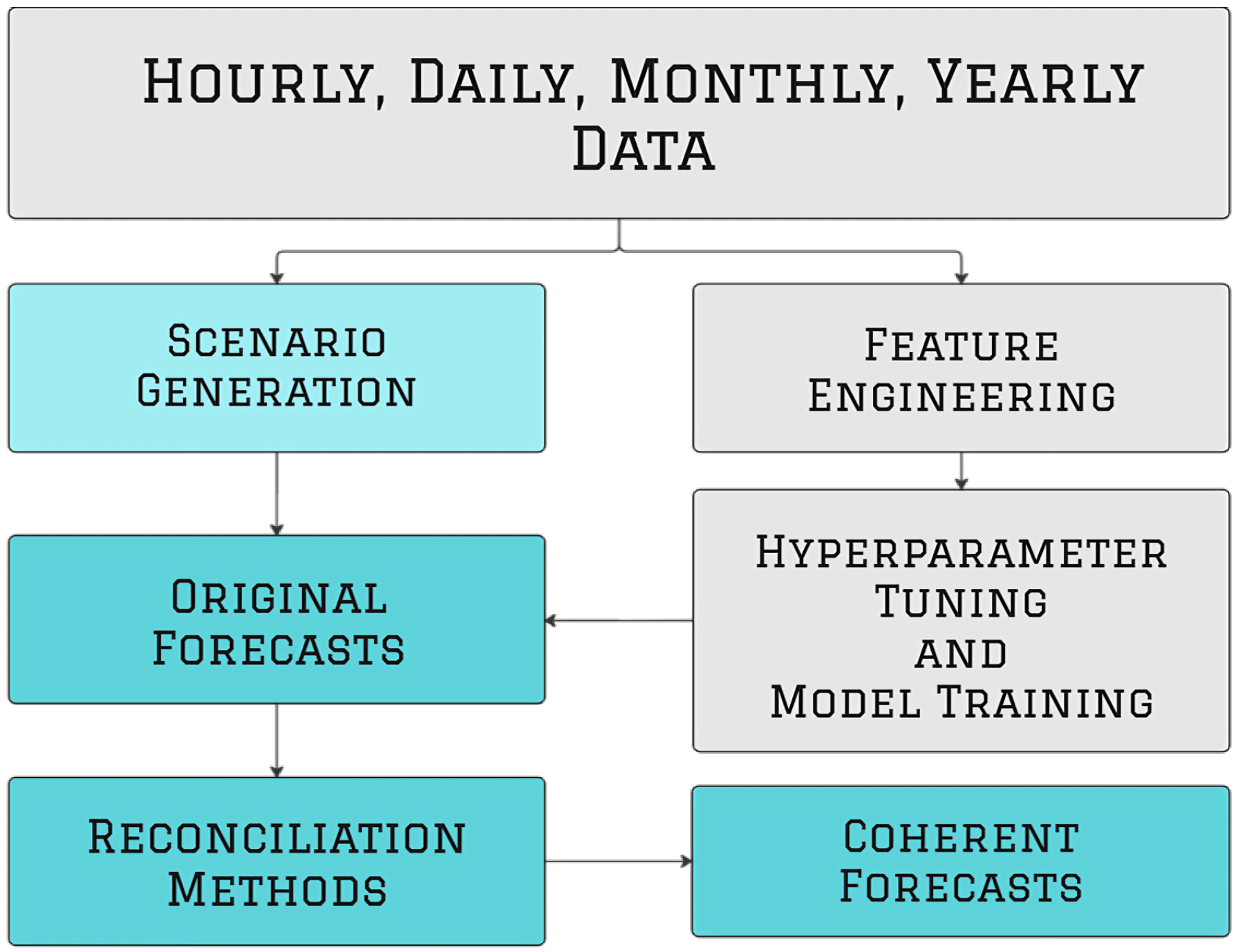
Figure 1 illustrates the block diagram of the proposed method. First, feature engineering is performed across all resolutions. Following Algorithm A1, new features are generated from the available data. Because an excessive number amount of features results in overfitting on the part of the models, a feature selection step in included in Algorithm A2. Feature selection is conducted independently for each resolution, acknowledging that different temporal scales (e.g., hourly, yearly) are influenced by distinct underlying drivers. For example, hourly forecasts may rely on weather and calendar effects, while yearly forecasts emphasize economic and demographic indicators. For each resolution, we use XGBoost’s gain-based feature importance to rank the predictors and apply a recursive elimination process similar to recursive feature elimination (RFE), removing the least important features one at a time. Model performance is evaluated after each iteration using rolling-origin backtesting with five years of training and one year of validation, which is repeated 13 times by monthly shifting of the origin. This approach mitigates overfitting and allows out-of-sample performance to guide feature selection. In the yearly resolution, the number of observations is small; thus, we begin with a limited number of aggregated features and apply a conservative pruning strategy to ensure model simplicity and reduce the risk of overfitting.

Each resolution is modeled independently using the features and algorithms best suited to its temporal scale while reflecting the distinct patterns and drivers at each level. Rather than assuming consistency across resolutions, we enforce it through a reconciliation step that adjusts the independently generated forecasts into a coherent system, as illustrated in Figure 1. XGBoost and ARIMAX are selected as the base forecasting models for the temporal hierarchy due to their demonstrated effectiveness in long-term load forecasting applications. XGBoost is a tree-based ensemble learning algorithm that has been widely used for its ability to model nonlinear relationships and interactions in high-resolution time series data. Electricity load data are influenced by weather, calendar effects, and behavioral factors [44,45,46]. XGBoost’s scalability and interpretability make it well suited for applications requiring fine-grained forecasts, including prediction of hourly, daily, and monthly loads. In contrast, annual load forecasts typically contain fewer observations and exhibit smoother long-term trends driven by macroeconomic indicators. For this reason, we employ ARIMAX at the annual resolution. ARIMAX is a classical time series model that incorporates exogenous variables. It remains a competitive choice for long-horizon forecasting due to its robustness, simplicity, and strong performance in capturing long-term trends [34,47]. Together, these two models provide a stable and interpretable foundation for the hierarchical reconciliation framework proposed in this work. Algorithm A3 shows the procedure for tuning and training the models for all resolutions.

Temperature and economic scenarios generated with Algorithm A4 are used to generate the ex ante probabilistic forecasts, with deterministic forecasts derived as the mean using Algorithm A5. Economic scenarios are based on historical trends and growth scenarios, while temperature scenarios are based on historical values and shifting. After the original forecasts are generated, reconciliation methods are applied following Algorithm A6 to ensure coherence across the various temporal resolutions.

3.2. Hierarchical Modeling and Reconciliation

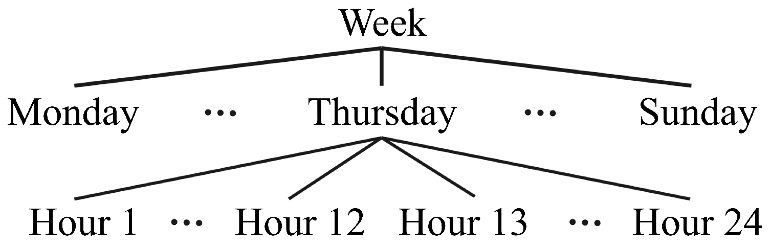
When data have a hierarchical structure, such as the structure displayed in Figure 2, hierarchical modeling and reconciliation methods can be used to improve forecasts. The figure illustrates a temporal hierarchy; in this case, the highest level is a time series with a frequency of one week, while the second and third levels have frequencies of days and hours, respectively.

Considering a time series $\{y_t^{\left[1\right]};t=1,2,3,\dots ,T\}$ with the highest resolution, in this case hourly, the number of series at the bottom level is $m=168$. The k-aggregates can be constructed from $y_t$, where k is a factor of m. The total number of series in the hierarchy is $n=1+7+168=176$. The various aggregated series can be written as [21]

$$\begin{array}{c}\hfill y_j^{\left[k\right]}=\sum _{t=t^{*}+jk-k}^{t^{*}+jk-1}{y}_t,\end{array}$$

(1)

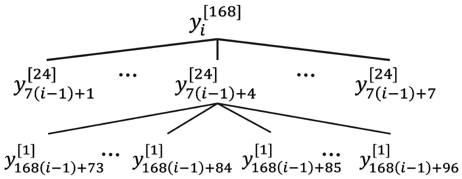
where j ranges from 1 to $\lfloor T/k\rfloor$, k belongs to $\{k_1,k_2\dots ,k_p=m\}$, and $t^{*}=T-\lfloor T/k\rfloor m+1$. Using Equation (1), each series in the hierarchy in Figure 2 can be expressed as $y_{M_k(i-1)+{\delta }_k}^{\left[k\right]}$, where i ranges from 1 to $\lfloor T/m\rfloor$, $M_k=m/k$ and ${\delta }_k=1,2,\dots ,M_k$. Figure 3 shows the new expression for the hierarchy using the common index i. We obtain the vector of all observations in the hierarchy as ${\mathit{y}}_{\mathit{i}}=\left[y_{M_k(i-1)+{\delta }_k}^{\left[k\right]}\right]$, where ${\delta }_k\in \{1,2,\dots ,M_k\}$ and the vector of all observations in the lowest level of hierarchy is ${\mathit{\beta }}_{\mathit{i}}=\left[y_{m(i-1)+{\delta }_1}^{\left[1\right]}\right]$, where ${\delta }_1\in \{1,2,\dots ,m\}$. Now, we have

$$\begin{array}{c}\hfill {\mathit{y}}_{\mathit{i}}=\mathbf{S}{\mathit{\beta }}_{\mathit{i}},\end{array}$$

(2)

where $\mathbf{S}$ is an $n\times m$ matrix called the summing matrix [43].

The reconciliation problem can be considered as a combination of direct forecasts of each time series, with additional indirect forecasts derived from the linear constraints resulting from the relation between the time series; in other words, each aggregation level in the hierarchy is forecasted separately and the results are reconciled to obtain coherent forecasts. Here, ${\widehat{\mathit{y}}}_{\mathit{h}}$ is the vector of all forecasts for any h-step horizon at the highest level of the hierarchy and ${\tilde{\mathit{y}}}_{\mathit{h}}$ is the vector of reconciled forecasts:

$$\begin{array}{c}\hfill {\tilde{\mathit{y}}}_{\mathit{h}}=\mathbf{S}\mathbf{G}{\widehat{\mathit{y}}}_{\mathit{h}}\end{array}$$

(3)

where $\mathbf{G}$ represents the mapping matrix applied in different reconciliation methods, as described by [17]. The bottom-up method starts with forecasts at the lowest level of the hierarchy and aggregates them to produce forecasts for higher levels; conversely, the top-down method begins with a forecast at the highest level, which is then disaggregated down to lower levels. In the middle-out approach, forecasts are generated at an intermediate level of the hierarchy, then disaggregated to lower levels and aggregated to higher levels as needed. Lastly, the optimal reconciliation method independently forecasts each hierarchical level and then adjusts these forecasts to ensure coherency across levels. This adjustment is optimized to minimize the overall forecast error.

3.3. Deterministic Forecast Reconciliation

The objective of a reconciliation method is to determine the optimal matrix $\mathbf{G}$. In the case of optimal reconciliation, the best matrix $\mathbf{G}$ is the one that minimizes the error variances of the coherent forecasts. With $h^{*}$ as the maximum required forecast horizon at the lowest level of the hierarchy (highest resolution) and h as the forecast horizon required at the highest level of the hierarchy (lowest resolution), the variance–covariance matrix of the h-steps-ahead coherent forecast errors is provided as follows [43]:

$$\begin{array}{c}\hfill V_h=Var[y_{T+h}-{\tilde{y}}_h]=\mathbf{S}\mathbf{G}{\mathbf{W}}_h{\mathbf{G}}^{\prime }{\mathbf{S}}^{\prime }\end{array}$$

(4)

where ${\mathbf{W}}_h=Var\left[(y_{T+h}-{\widehat{y}}_h)\right]$ is the variance–covariance matrix of the original forecast errors. Now, we have

$$\begin{array}{c}\hfill \mathbf{G}={\left({\mathbf{S}}^{\prime }{\mathbf{W}}_h^{-1}\mathbf{S}\right)}^{-1}{\mathbf{S}}^{\prime }{\mathbf{W}}_h^{-1}.\end{array}$$

(5)

To find the best matrix $\mathbf{G}$, we need the variance–covariance matrix ${\mathbf{W}}_h$ in Equation (5). If ${\mathbf{W}}_h$ were known, the problem could be easily solved using a generalized least squares (GLS) estimator. However, knowing the exact ${\mathbf{W}}_h$ relies on knowing the actual forecast error values, which is not possible. Thus, we instead estimate ${\mathbf{W}}_h$. A straightforward approach involves using an ordinary least squares (OLS) estimator and assuming ${\mathbf{W}}_h={\sigma }^2\mathbf{I}$.

An alternative approach is to use weighted least squares (WLS), which uses in-sample forecast errors to estimate ${\mathbf{W}}_h$. Defining the in-sample one-step-ahead original forecast errors as $e_i={({e_i^{\left[m\right]}}^{\prime },\dots ,{e^{\left[k_2\right]}}^{\prime },{e^{\left[k_1\right]}}^{\prime })}^{\prime }$ for $i=1,\dots ,\lfloor T/m\rfloor$, we have

$$\begin{array}{c}\hfill {\mathbf{W}}_h=k_h\mathsf{\Lambda },\end{array}$$

(6)

where $k_h\ge 0$ and

$$\begin{array}{c}\hfill \mathsf{\Lambda }={\displaystyle \frac{1}{\lfloor T/m\rfloor }}\sum _{i=1}^{\lfloor T/m\rfloor }{e}_i{e}_i.\end{array}$$

(7)

Two specific alternatives to the WLS method for temporal hierarchies were introduced by [21]. The series variance scaling (WLS_V) method assumes that the forecast error variances are consistent within each level of a temporal hierarchy, as they correspond to the same time series. This assumption reduces the number of variances that need to be estimated to the number of aggregation levels. Here, ${\mathsf{\Lambda }}_V$ is a diagonal matrix that contains estimates of the in-sample one-step-ahead error variances across each level. In addition to the assumptions from (WLS_V), the structural scaling (WLS_S) method assumes that the bottom-level original forecast error variance is ${\sigma }^2$ and that ${\mathbf{W}}_h$ is set to ${\sigma }^2\times {\mathsf{\Lambda }}_S$, where ${\mathsf{\Lambda }}_S$ is a diagonal matrix with each element containing the number of forecast errors contributing to that aggregation level:

$$\begin{array}{c}\hfill {\mathsf{\Lambda }}_S=diag\left(\mathbf{S}\mathbf{1}\right)\end{array}$$

(8)

where $\mathbf{1}$ is a unit column vector with a dimension of m. In this way, only one variable estimate is needed.

Two other alternatives for ${\mathbf{W}}_h$ were presented by [43], called Mint(sample) and Mint(shrink). In the MinT(sample) method, ${\mathbf{W}}_h=k_h{\mathbf{W}}_1$. This approach is not recommended when the number of bottom-level series m is large relative to the series length T. In the MinT(shrink) method, ${\mathbf{W}}_h=k{\mathbf{W}}_{1,D}^{*}$, where ${\mathbf{W}}_{1,D}^{*}={\lambda }_D{\mathbf{W}}_D+(1-{\lambda }_D){\mathbf{W}}_{1,D}$. Here, ${\mathbf{W}}_D$ is a diagonal matrix comprising the diagonal entries of ${\mathbf{W}}_1$, while ${\lambda }_D$ is the shrinkage intensity parameter. when the shrinkage intensity parameter is high, this method is similar to the WLS_V method.

In this paper, the MinT(shrink) method is deployed along with OLS, WLS_S, WLS_V, and a simple bottom-up reconciliation approach as benchmarks in a temporal hierarchy structure for the proposed long-term load forecasting model. Our goal is to produce a one-year-ahead load forecast with four aggregation levels—hourly, daily, monthly, and yearly—leveraging information from each resolution.

We exclude the MinT(sample) method from our analysis, as in our case $h=1$, making MinT(sample) equivalent to the WLS approach. Additionally, given that $m=8760$ and T = 87,600, MinT(sample) is unsuitable. We implement these reconciliation methods using the Python Hierarchical Forecast library developed by [42].

The reconciliation methods used in this study rely on key assumptions about the statistical properties of forecast errors. In particular, WLS-based methods assume that reconciliation weights can be estimated using a known or estimable variance–covariance matrix of base forecast errors. We follow standard practice by estimating this matrix using in-sample residuals under the assumption of approximate normality and temporal independence [48]. To evaluate the impact of this assumption, we also explore an alternative approach that estimates the variance structure from out-of-sample forecast errors. This method, labeled WLS_V-OSE, provides a more realistic treatment of forecast uncertainty in long-horizon settings.

This analysis aims to evaluate the effectiveness of reconciliation methods in producing coherent long-term deterministic load forecasts in both ex post and ex ante approaches. In addition to deterministic forecasts, our approach produces probabilistic forecasts, which also require reconciliation to ensure consistency across temporal levels. Although real-world load forecast errors may exhibit skewness or seasonality, the Gaussian assumption enables computationally efficient reconciliation and has shown strong empirical performance in prior studies.

3.4. Probabilistic Forecast Reconciliation

According to [27], for an h-steps-ahead probabilistic forecast presented as $\mathcal{N}({\widehat{y}}_T+h,{\mathbf{W}}_h)$, where ${\widehat{y}}_T+h$ is the mean h-steps-ahead forecast and

$$\begin{array}{c}\hfill {\mathbf{W}}_h=E[y_T+h-{\widehat{y}}_T+h]{[y_T+h-{\widehat{y}}_T+h]}^T,\end{array}$$

(9)

there is a matrix $\mathbf{G}$ that produces

$$\begin{array}{c}\hfill \mathcal{N}(\mathbf{S}\mathbf{G}{\widehat{y}}_T+h,\mathbf{S}\mathbf{G}{\mathbf{W}}_h{\mathbf{G}}^T{\mathbf{S}}^T),\end{array}$$

(10)

which represents the h-steps-ahead reconciled forecast. Assuming that the predictive densities of the original forecasts follow a Gaussian distribution, the same matrix $\mathbf{G}$ used for reconciling point forecasts can also be employed for probabilistic forecasts. Therefore, the reconciliation methods used for deterministic forecasts are extended to probabilistic forecast reconciliation in this study.

Our probabilistic reconciliation is based on the Gaussian assumption, as proposed by [27], where the forecast distribution is assumed to follow a multivariate normal distribution. This permits closed-form reconciliation through linear algebraic transformation.

4. Experimental Setup and Empirical Evaluation Results

This section outlines the experimental setup and empirical evaluation of our proposed long-term load forecasting model. We utilize electricity demand data from the cities of Calgary and Edmonton as well as from the province of Alberta, Canada to assess the model’s performance. The evaluation focuses on various forecasting scenarios, encompassing both deterministic and probabilistic approaches. We detail the data sources and characteristics, the generation of weather and economic scenarios, and the evaluation metrics employed to measure the model’s reliability. The results from deterministic and probabilistic forecasts are discussed, highlighting the effectiveness of reconciliation approaches in producing coherent forecasts in a temporal hierarchy.

4.1. Data

We extracted the historical hourly load data for the cities of Calgary and Edmonton and for the province of Alberta from [49,50] for the period of 2012–2024. For our analysis, we used six years of data for training and applied a monthly rolling validation strategy over the following year. This process was repeated to span three years of validation, enabling effective model tuning. The hourly load from the next available year (2020) was used for out-of-sample testing. This process was repeated for the next three years to produce one-year ahead out-of-sample load forecasts for four years, and the results are reported for the combination of all four years.

The three datasets used in this study—Calgary, Edmonton, and the province of Alberta—each represent distinct load characteristics. Calgary and Edmonton primarily reflect residential and commercial consumption patterns typical of urban centers, while the Alberta-wide dataset is dominated by industrial demand. This diversity in load composition allows for the evaluation of forecasting and reconciliation methods across a wide range of demand behaviors. Although the data are geographically limited to one jurisdiction, the variation in load types makes the case study more broadly informative.

The available information is presented at various resolutions. Historical economic variables are typically available at yearly, quarterly, and monthly frequencies. We incorporated economic data from [51] alongside long-term climate trends for monthly and yearly load forecasting. Weather-related variables [52] are available at higher resolutions, and are utilized in forecasting hourly and daily loads.

Table 1. Information used for forecasting loads in different resolutions.

Feature Type	Feature Group	Hourly Load	Daily Agg	Monthly Agg	Yearly Agg
Time Related	Calendar dummy variables	✓	✓	✓	✓
	Day light	✓	✓	✗	✗
Weather related	Temperature	✓	a,b,c	a,b,c	a
	Humidity	✓	a	a	✗
	Pressure	✓	a	a	✗
	Solar radiation	✓	a	a	✗
	Wind	✓	a	a	✗
	Precipitation	✓	a	a	✗
Economy related	GDP	✗	✗	✗	✓
	Population	✗	✗	✗	✓
	Productivity	✗	✗	✗	✓
	Income	✗	✗	✓	✗
	Inflation	✗	✗	✓	✗
	Unemployment	✗	✗	✓	✗
	Housing	✗	✗	✓	✗
	Drills	✗	✗	✓	✗
	Oil & Gas production	✗	✗	✓	✗

Note: a: Averaged value of a variable in specific periods. b: Maximum value of a variable in specific periods. c: Minimum value of a variable in specific periods.

outlines the information groups used for load forecasting at each resolution. Each group consists of one or more variables of a similar nature; for instance, solar radiation and visibility are categorized together. To enhance the model’s predictive capability, we included squared and cubed forms of weather variables as well as their interactions with dummy variables such as hour of the day and day of the week.

To ensure data quality and robust evaluation, we performed preprocessing on all input series. Missing values were filled using forward-filling and seasonal mean backfilling. Outliers were detected for the training period only using interquartile range (IQR)-based filtering and replaced with local median values. Numerical features were standardized within each resolution level to control for scale effects. Importantly, the one-year-ahead forecasting process was repeated across four independent test years for each region (Calgary, Edmonton, and Alberta), providing a robust basis for generalization and mitigating the risk of overfitting to a single forecast year. The consistency of performance improvements across these multi-year and multi-region experiments reinforces the robustness of the framework under varying conditions and input distributions.

4.2. Scenario Generation

Probabilistic forecasts can be derived from various scenarios, especially when producing ex ante forecasts where input data such as weather variables for the forecasting period are unavailable. In this context, scenario generation methods are employed to facilitate the production of probabilistic forecasts. Weather-related variables are particularly crucial in load forecasting, and using simulated weather scenarios in point load forecasting models has gained widespread acceptance in the industry thanks to its simplicity and ease of interpretation.

As outlined by [12], weather scenario simulation methods range from straightforward to more complex approaches. The simplest method directly uses the original historical weather data, while a moderate approach involves reorganizing the data through techniques such as rotation or bootstrapping. The most advanced methods entail simulating historical weather patterns using mathematical models, such as applying Fourier transformation to the original weather series to generate additional scenarios. The first two methods are practical and widely used in industry [12]. However, given the limited availability of historical hourly data, the first approach results in a restricted number of scenarios. Therefore, we opt here for the modest approach to temperature scenario generation.

Specifically, we used rotation of historical weather data to generate 200 weather scenarios for hourly and daily forecasts. The same method was applied to produce 50 monthly and yearly weather scenarios alongside four economic growth scenarios (normal growth, double growth, no growth, and negative growth), leading to a total of 200 scenarios. The resulting forecasts from these scenarios for each resolution were then utilized to construct the probability density function for the probabilistic forecasts, with the mean value of these probability density functions serving as the deterministic forecasts.

4.3. Evaluation Metrics

Evaluation of deterministic forecasts is conducted using the root mean square error (RMSE) metric. The RMSE is particularly sensitive to outliers, such as sudden peak loads in our case, making it an appropriate choice for assessing our results. For the evaluation of probabilistic forecasts, we utilize the Pinball loss function and Winkler score, both of which are widely recognized in the field of probabilistic forecast evaluation.

The Pinball loss function serves as an error measure that accounts for both sharpness and resolution in quantile forecasts. Let ${\widehat{y}}_{t,q}$ denote the load forecast at the $q_{th}$ quantile and let $y_t$ represent the actual load value observed; then, the Pinball loss function can be expressed as follows [13].

$$\begin{array}{c}\hfill P({\widehat{y}}_{t,q},y_t,q)=\left\{\begin{array}{cc}(1-q)({\widehat{y}}_{t,q}-y_t)\hfill & y_t<{\widehat{y}}_{t,q}\hfill \\ q(y_t-{\widehat{y}}_{t,q})\hfill & y_t\ge {\widehat{y}}_{t,q}\hfill \end{array}\right.\end{array}$$

(11)

The Winkler score allows for a joint assessment of unconditional coverage and interval width. For a central $(1-\alpha )\times 100\%$ prediction interval, $\left[l_{\alpha ,t},u_{\alpha ,t}\right]$ it is defined as follows [43].

$$\begin{array}{c}\hfill \mathrm{W}=\left\{\begin{array}{cc}(u_{\alpha ,t}-l_{\alpha ,t})+{\displaystyle \frac{2}{\alpha }}(l_{\alpha ,t}-y_t)\hfill & y_t<l_{\alpha ,t}\hfill \\ (u_{\alpha ,t}-l_{\alpha ,t})\hfill & l_{\alpha ,t}\le y_t\le u_{\alpha ,t}\hfill \\ (u_{\alpha ,t}-l_{\alpha ,t})+{\displaystyle \frac{2}{\alpha }}(y_t-u_{\alpha ,t})\hfill & y_t>u_{\alpha ,t}\hfill \end{array}\right.\end{array}$$

(12)

We calculate both the Pinball and Winkler scores for all four resolutions as well as for the daily, monthly, and yearly peak loads.

4.4. Deterministic Ex Post Forecasts

Three years of out-of-sample feature values used for forecasting load are utilized to generate forecasts across various resolutions. The hourly load forecast is subsequently used to extract daily, monthly, and yearly peak loads. A range of reconciliation methods, including bottom-up, MinT(shrink), ordinary least squares (OLS), weighted least squares (WLS)_S, and WLS_V, are employed to generate coherent forecasts. These methods leverage in-sample forecast errors; additionally, we apply out-of-sample errors with the WLS_V method to reconcile the forecasts. The performance of each method is evaluated by comparing the RMSE of the coherent forecasts against the RMSE of the original forecasts. The Clark–West (CW) test is used to check the statistical significance of the improvements in the forecasts after reconciliation compared to the original forecasts. Ex post and ex ante forecast results are reported separately and should not be compared directly, as they rely on different information availability at forecast time.

Table 2. Percentage improvements in RMSE for ex post deterministic forecast for the City of Calgary.

Load Type	Bottom-Up	OLS	WLSS	WLSV	WLSV-OSE
Hourly Load	0.00	0.13 *	0.71 *	0.56 *	−0.37 *
Daily Aggregated	0.84 *	1.02 *	1.78 *	1.64 *	0.65 *
Monthly Aggregated	2.27	1.92	4.02 *	5.02 *	1.28
Yearly Aggregated	−65.06	3.37	−28.09	−23.37	−62.71
Daily Peak	0.00	0.91 *	0.69 *	0.26 *	−0.34 *
Monthly Peak	0.00	−0.09 *	−1.99 *	−0.92 *	0.55
Yearly Peak	0.00	1.40	−1.39	−3.33	3.87

Note: Each value shows the RMSE percentage improvement compared to the original forecast. * denotes statistical significance at the 0.05 level (Clark–West test). Bold values indicate the best performance (highest improvement) for each load type. The out-of-sample error is used for WLS_V-OSE.

,

Table 3. Percentage improvements in RMSE for ex post deterministic forecast for the City of Edmonton.

Load Type	Bottom-Up	OLS	WLSS	WLSV	WLSV-OSE
Hourly Load	0.00	−1.19 *	0.83 *	−0.14 *	−0.15 *
Daily Aggregated	0.92	−0.57	1.96 *	0.83 *	0.88
Monthly Aggregated	−4.87 *	−9.63	−1.52 *	−5.21 *	−4.66 *
Yearly Aggregated	21.34	6.02 *	30.47 *	22.32	23.63
Daily Peak	0.00	−0.16	0.91 *	−0.13 *	−0.33 *
Monthly Peak	0.00	3.50	1.23 *	−0.26 *	−0.17 *
Yearly Peak	0.00	3.88	−0.81	−1.38	−0.06

Note: Each value shows the RMSE percentage improvement compared to the original forecast. * denotes statistical significance at the 0.05 level (Clark–West test). Bold values indicate the best performance (highest improvement) for each load type. The out-of-sample error is used for WLS_V-OSE.

and

Table 4. Percentage improvements in RMSE for ex post deterministic forecast for the Province of Alberta.

Load Type	Bottom-Up	OLS	WLSS	WLSV	WLSV-OSE
Hourly Load	0.00	−10.50 *	12.80 *	1.32 *	0.80 *
Daily Aggregated	−10.90 *	−24.17 *	5.58 *	−9.16 *	−8.42 *
Monthly Aggregated	−28.58 *	−47.80	6.55 *	−25.36 *	−21.77 *
Yearly Aggregated	23.31 *	5.70 *	59.84 *	26.43 *	30.31 *
Daily Peak	0.00	−6.77 *	14.90 *	1.81 *	−1.32 *
Monthly Peak	0.00	−1.17 *	19.49 *	2.85 *	−12.69 *
Yearly Peak	0.00	55.42 *	37.13 *	3.95	−76.82 *

Note: Each value shows the RMSE percentage improvement compared to the original forecast. * denotes statistical significance at the 0.05 level (Clark–West test). Bold values indicate the best performance (highest improvement) for each load type. The out-of-sample error is used for WLS_V-OSE.

present the relative percentage improvements in RMSE scores for ex post deterministic forecasts across different reconciliation methods compared to the original forecasts. A positive percentage indicates a decrease in the RMSE value, suggesting that the original forecast is superior to the reconciled forecast, while a negative percentage reflects an increase in RMSE. Notably, the MinT(shrink) and WLS_V methods yield remarkably similar results, with less than a 0.001% difference across all datasets. This can be a result of a high shrinkage intensity parameter. Thus, only the results for WLS_V are reported in the tables.

While improvements in forecast accuracy through reconciliation are certainly beneficial, they are not the primary objective. The main goal of reconciliation methods is to ensure coherence across forecasts. Therefore, the focus is on comparing the results of various reconciliation methods with the simple bottom-up approach.

Table 2 presents the results for ex post deterministic forecasts in Calgary. The results show that all methods except WLS_V-OSE achieve statistically significant improvements in RMSE at the hourly, daily aggregated, and daily peak levels, as indicated by the dagger symbols. The best performance at each frequency is generally achieved by either WLS_S or WLS_V, particularly for hourly and daily resolutions, with the OLS and bottom-up methods also showing significant but smaller improvements. For monthly and yearly aggregates and peaks, improvements are less often statistically significant. While both WLS_V and WLS_V-OSE show similar trends, there is no clear evidence of consistent superiority of either method in this setting.

Overall, these results support the benefit of reconciliation for improving the coherence and accuracy of ex post deterministic forecasts in Calgary, particularly OLS and WLS_S, with statistical evidence showing that most improvements are meaningful rather than due to random variability. Notably, these results highlight that the extent of improvement and significance can vary substantially by aggregation level and load type.

The ex post deterministic forecasting results for the City of Edmonton, shown in Table 3, reveal meaningful improvements in RMSE across several reconciliation methods and aggregation levels. The WLS_S method yields the highest and statistically significant RMSE improvements for most load types, particularly for hourly, daily aggregated, and yearly aggregated loads. In the case of monthly aggregated loads, WLS_S still provides the least negative (best) result among methods, with significance also observed for bottom-up, WLS_V, and WLS_V-OSE. For hourly, daily, and monthly peak loads, WLS_S again shows the largest improvements, most of which are statistically significant. The OLS method occasionally shows significance, notably in yearly aggregated and monthly peak loads, but with lower improvements compared to WLS-based approaches.

When comparing WLS_V and WLS_V-OSE (the latter using out-of-sample error for reconciliation), their performance is generally similar across most load types. The difference in RMSE improvement between WLS_V and WLS_V-OSE remains small for most metrics, and both methods show comparable significance patterns. These results suggest that in the context of Edmonton’s long-term forecasting, employing out-of-sample errors for WLS-based reconciliation does not lead to substantial changes in performance.

The ex post deterministic results for the province of Alberta, shown in Table 4, reveal that reconciliation methods can provide substantial improvements in RMSE for many load types and aggregation levels. This is particularly the case for WLS_S, with the majority of improvements being statistically significant (p < 0.05). WLS_S delivers the highest improvements overall, achieving double-digit gains for hourly, yearly aggregated, daily peak, monthly peak, and yearly peak forecasts. Similar to the other two cases, employing out-of-sample errors in the reconciliation process does not substantially alter the forecast improvements compared to using in-sample errors.

The results indicate that employing a temporal hierarchy structure can enhance the accuracy of ex post deterministic forecasts while ensuring coherence across forecasts. It is obvious that the performance of reconciliation methods varies across datasets. The difference in performance can be related to the composition of load in each dataset, although this needs to be investigated further in the future. Considering all of these results, the WLS_S method consistently improves forecast performance for hourly and daily loads as well as daily peak loads in all three datasets.

Although methods such as WLS_V are typically designed for situations where using out-of-sample errors is challenging or infeasible, our findings indicate that incorporating out-of-sample errors only rarely improves forecast performance, and in many cases can actually reduce forecast accuracy.

It is important to note when using reconciliation methods that there can be a deterioration in forecast performance compared to the original forecasts, particularly at higher levels of the temporal hierarchy. Nonetheless, the primary objective is to produce coherent forecasts across all hierarchy levels. The simplest way to achieve this is through the bottom-up approach. Our results demonstrate that optimal reconciliation methods such as WLS_S yield better forecasts compared to the bottom-up approach.

4.5. Deterministic Ex Ante Forecasts

While ex post forecasts are excellent for comparing model performance by isolating the external error effects, ex ante forecasts are more practical and useful in industrial contexts. While ex post forecasts are affected by errors in the forecasting model, ex ante forecasting must additionally face the problem of input errors. Ex ante deterministic forecasts are derived by calculating the mean values of the probability distributions from the scenario-based probabilistic forecasts. The combined results for four years of one-year-ahead ex ante load forecasts are presented in

Table 5. Percentage improvements in RMSE for ex ante deterministic forecast for the City of Calgary.

Load Type	Bottom-Up	OLS	WLSS	WLSV	WLSV-OSE
Hourly Load	0.00	2.83 *	4.69 *	1.44 *	1.08 *
Daily Aggregated	−6.76	−2.84 *	−0.24 *	−4.77	−5.12
Monthly Aggregated	−5.02 *	1.16	9.06 *	−0.86 *	−1.39 *
Yearly Aggregated	−4.67 *	−0.30	40.75	12.01	0.53
Daily Peak	0.00	1.44 *	3.61 *	1.04 *	1.37 *
Monthly Peak	0.00	2.29	3.47 *	1.43 *	6.77 *
Yearly Peak	0.00 *	1.01 *	−0.57 *	−0.19 *	0.53 *

Note: Each value shows the RMSE percentage improvement compared to the original forecast. * denotes statistical significance at the 0.05 level (Clark–West test). Bold values indicate the best performance (highest improvement) for each load type. The out-of-sample error is used for WLS_V-OSE.

,

Table 6. Percentage improvements in RMSE for ex ante deterministic forecast for the City of Edmonton.

Load Type	Bottom-Up	OLS	WLSS	WLSV	WLSV-OSE
Hourly Load	0.00	4.45 *	4.97 *	1.43 *	0.56 *
Daily Aggregated	−4.95	0.85 *	1.53 *	−3.01	−4.19
Monthly Aggregated	−9.91	0.30	4.77 *	−5.17	−8.35
Yearly Aggregated	−30.20	1.36	6.57	−14.35	−31.43
Daily Peak	0.00	−0.77 *	2.77 *	0.88 *	0.77 *
Monthly Peak	0.00	−5.93	−0.21	0.28	3.50 *
Yearly Peak	0.00	−11.04	−6.47	−0.89	−0.13

Note: Each value shows the RMSE percentage improvement compared to the original forecast. * denotes statistical significance at the 0.05 level (Clark–West test). Bold values indicate the best performance (highest improvement) for each load type. The out-of-sample error is used for WLS_V-OSE.

and

Table 7. Percentage improvements in RMSE for ex ante deterministic forecast for the Province of Alberta.

Load Type	Bottom-Up	OLS	WLSS	WLSV	WLSV-OSE
Hourly Load	0.00	27.48 *	22.70 *	0.09 *	−0.75
Daily Aggregated	13.45 *	39.53 *	34.92 *	13.54 *	12.81 *
Monthly Aggregated	−50.42	6.12 *	−5.01	−50.36	−51.78
Yearly Aggregated	−157.86	7.25 *	−57.79	−157.88	−161.01
Daily Peak	0.00	40.77 *	23.19 *	0.26 *	−0.34
Monthly Peak	0.00	44.57 *	20.86 *	0.63 *	0.79
Yearly Peak	0.00	54.97 *	18.04 *	0.84	−0.09

Note: Each value shows the RMSE percentage improvement compared to the original forecast. * denotes statistical significance at the 0.05 level (Clark–West test). Bold values indicate the best performance (highest improvement) for each load type. The out-of-sample error is used for WLS_V-OSE.

.

Table 5 presents RMSE improvements for ex ante deterministic forecasts in Calgary. The results indicate that the reconciliation methods deliver significant improvements in RMSE at several aggregation levels, particularly WLS_S and OLS. Most p-values are below 0.05, confirming statistical significance. WLS_S provides the largest and most consistent gains, especially for hourly (4.69%) and monthly (9.06%) aggregated loads. In particular, improvements are also significant for daily and monthly peaks in most reconciliation approaches. In contrast, negative or small improvements are observed for daily and monthly aggregates under some methods, with these changes generally being statistically significant as well. The difference between WLS_V and WLS_V-OSE is minimal, with both delivering similar results. In general, these findings highlight the strong benefits of reconciliation, especially WLS_S, in improving the precision of long-term ex ante forecasts for most resolutions and load types.

Table 6 shows RMSE improvements for ex ante deterministic forecasts in Edmonton. Notable improvements in RMSE are apparent, especially for hourly and monthly aggregated loads. WLS_S consistently provides the largest percentage improvement for most load types (e.g., 4.97% for hourly and 4.77% for monthly), with OLS also yielding statistically significant gains across hourly and daily aggregated categories. The improvements for hourly, daily, and daily peak loads are generally supported by p-values below 0.05, indicating robust statistical significance. Some negative improvements are observed for daily and monthly aggregates under certain methods; however, they are not statistically significant. The results for WLS_V and WLS_V-OSE are similar, and neither approach provides substantial additional benefit over WLS_S. Overall, the findings for Edmonton highlight the effectiveness of reconciliation, particularly WLS_S and OLS, for improving ex ante forecast accuracy across most resolutions.

For ex ante deterministic forecasts in Alberta (Table 7), the reconciliation methods deliver large and statistically significant improvements in RMSE at most resolutions, particularly OLS and WLS_S. OLS achieves the highest gains in nearly every category, notably for hourly (27.48%), daily (39.53%), and yearly peak (54.97%) loads. All corresponding p-values are below 0.05, confirming the significance of these improvements. WLS_S also yields substantial and significant improvements, especially for hourly, daily aggregated, and peak loads in every level. For aggregated monthly and yearly series, most methods actually show negative improvements, reflecting a loss of accuracy, though OLS still provides small but significant gains. The WLS_V and WLS_V-OSE methods generally do not offer additional improvement over OLS or WLS_S, and sometimes result in negative or negligible changes. These results highlight the robust advantage of OLS and WLS_S reconciliation for high- and mid-resolution load forecasting in Alberta, with performance on monthly and yearly aggregation being more method-dependent.

While reconciliation typically provides overall coherence and often enhances forecast accuracy across levels, there are cases where performance at a specific resolution may degrade. For example, when the original forecast at a particular level (e.g., yearly) is already highly accurate, the reconciliation step may shift values to ensure consistency with forecasts at other levels, resulting in a tradeoff. This behavior is expected and aligns with findings in the prior hierarchical forecasting literature. Furthermore, large percentage increases in RMSE may correspond to relatively small absolute errors in certain cases, particularly when the baseline RMSE is low. These effects are not anomalies but are rather a consequence of the reconciliation objective prioritizing structural coherence over localized optimization.

The results indicate that there is no clear winner among the reconciliation methods for all levels of load forecasting. The only method that consistently improves hourly load and daily peak load forecasts across all datasets is the WLS_S method. In addition, it is important to note that using out-of-sample forecast errors instead of in-sample errors similar to ex post forecast reconciliation does not guarantee better forecasts.

4.6. Probabilistic Ex-Ante Forecasts

The Pinball and Winkler scores for all four resolution levels of the hierarchy as well as for peak load forecasts are calculated below.

Table 8. Percentage improvements in Pinball score for ex ante probabilistic forecast for the City of Calgary.

Load Type	Bottom-Up	OLS	WLSS	WLSV	WLSV-OSE
Hourly Load	−4.86 *	12.19 *	6.37 *	−2.33 *	−3.20 *
Daily Aggregated	−44.35	3.23 *	−13.08 *	−39.03	−40.54
Monthly Aggregated	−55.77	6.86	−11.23	−46.04	−48.76
Yearly Aggregated	−48.83	9.05	27.79	−11.12	−39.34
Daily Peak	−5.19	7.31 *	2.70 *	−3.44 *	−3.41
Monthly Peak	−4.92	5.02	1.31 *	−2.63 *	14.46 *
Yearly Peak	−5.83 *	1.19 *	−5.45 *	−6.19 *	15.79 *

Note: Each value shows the Pinball score percentage improvement compared to the original forecast. * denotes statistical significance at the 0.05 level (Diebold–Mariano test). Bold values indicate the best performance (highest improvement) for each load type. The out-of-sample error is used for WLS_V-OSE.

,

Table 9. Percentage improvements in Pinball score for ex ante probabilistic forecast for the City of Edmonton.

Load Type	Bottom-Up	OLS	WLSS	WLSV	WLSV-OSE
Hourly Load	−3.63 *	17.33 *	8.89 *	−0.16 *	−2.81 *
Daily Aggregated	−47.67 *	9.64 *	−12.60 *	−39.98	−45.34
Monthly Aggregated	−64.01 *	8.27	−17.92	−50.81	−61.30
Yearly Aggregated	−120.75	9.43	−28.58	−70.56	−121.73
Daily Peak	−3.19 *	8.62 *	5.31 *	−0.90 *	−2.18
Monthly Peak	−3.15 *	−5.60 *	−2.72	−2.83	10.02 *
Yearly Peak	−0.63	−7.57	−7.83	−2.02	11.95

Note: Each value shows the Pinball score percentage improvement compared to the original forecast. * denotes statistical significance at the 0.05 level (Diebold–Mariano test). Bold values indicate the best performance (highest improvement) for each load type. The out-of-sample error is used for WLS_V-OSE.

and

Table 10. Percentage improvements in Pinball score for ex ante probabilistic forecast for the Province of Alberta.

Load Type	Bottom-Up	OLS	WLSS	WLSV	WLSV-OSE
Hourly Load	−2.60 *	41.06 *	33.43 *	−2.44 *	−3.07 *
Daily Aggregated	−25.66 *	46.62 *	34.38 *	−25.21 *	−25.04 *
Monthly Aggregated	−131.95 *	17.64	−24.54	−131.68 *	−133.63 *
Yearly Aggregated	−377.10	11.92	−141.07	−376.28	−382.34
Daily Peak	−4.40	52.50 *	33.41 *	−4.10 *	−3.67 *
Monthly Peak	−4.96	59.16 *	29.32 *	−4.08 *	−5.95
Yearly Peak	−6.75	68.51 *	23.08 *	−5.97	17.49

Note: Each value shows the Pinball score percentage improvement compared to the original forecast. * denotes statistical significance at the 0.05 level (Diebold–Mariano test). Bold values indicate the best performance (highest improvement) for each load type. The out-of-sample error is used for WLS_V-OSE.

show the percentage relative improvements in the Pinball scores of different probabilistic reconciliation methods compared to the original forecasts. Because the Clark–West test is not designed for probabilistic forecasts, we use the Diebold–Mariano (DM) test to assess statistical significance. Unlike deterministic forecast reconciliation, where no single method consistently outperforms the others across datasets, the OLS method enhances the original hourly load forecast as well as daily, monthly, and yearly peak load forecasts in all three datasets.

Ex ante probabilistic forecasts in Calgary as measured by percentage improvements in Pinball score are presented in Table 8. OLS consistently delivers the most substantial and statistically significant gains, especially for hourly, daily, and peak load forecasts. For example, OLS improves the hourly Pinball score by 12.19%, daily aggregate by 0.23%, and daily peak by 7.31%, with all improvements being statistically meaningful at the 0.05 level. WLS_S also yields significant but smaller improvements for hourly, daily and monthly peak loads. In contrast, the bottom-up and WLS_V-based methods frequently result in negative improvements, with significantly worse Pinball scores for many horizons, particularly at aggregated and peak levels. Notably, OLS and WLS_V-OSE show meaningful positive gains for peak forecasts. Overall, OLS emerges as the most reliable reconciliation approach for improving the probabilistic accuracy of ex ante forecasts in Calgary, while other methods offer less consistent or even detrimental results across most resolutions.

Table 9 reports percentage improvements in Pinball score for ex ante probabilistic forecasts in Edmonton. Similar to the results for Calgary, OLS stands out by providing the largest and most statistically significant improvements in Pinball score across almost all horizons. OLS achieves an improvement of 17.33% for hourly load and 9.64% for daily aggregated load. WLS_S also demonstrates significant improvement for hourly and daily peak loads, with 8.89% and 5.31% improvement, respectively. However, for most aggregated and peak horizons, both the bottom-up and WLS_V-based methods yield negative or non-significant changes in Pinball score, often performing worse than the unreconciled forecast. Notably, the only consistent positive improvement for monthly and yearly peaks is observed for WLS_V-OSE (e.g., 10.02% for monthly peak). These results confirm that OLS is generally the most robust reconciliation method for enhancing the probabilistic accuracy of ex ante load forecasts for higher resolutions in Edmonton, while the other methods show inconsistent or often detrimental effects, especially for longer aggregation intervals.

Table 10 shows Pinball score improvements for ex ante probabilistic forecasts in Alberta. Both the OLS and WLS_S reconciliation methods achieve substantial and statistically significant improvements in Pinball score at nearly all resolutions, with OLS consistently providing the largest gains of over 40% improvement for hourly, daily, and peak intervals. The p-values for these methods are almost universally below 0.05, confirming that these improvements are meaningful. In contrast, WLS_V and WLS_V-OSE produce little to no improvement or even negative improvements across all resolutions and aggregation levels, and their performance does not significantly differ from each other. Bottom-up reconciliation generally results in negative improvements, especially at higher aggregation levels (e.g., monthly and yearly). These findings reinforce the effectiveness of OLS-based reconciliation in improving the accuracy of multi-resolution probabilistic load forecasts for large geographic regions.

Compared to the bottom-up method, the four reconciliation methods provide better results in almost all resolutions for the three datasets. While the OLS and WLS_S methods both improve upon the original hourly and daily peak forecasts, the OLS method is the only method that improves the forecasts for all aggregation levels. In addition, this method improves the peak load forecasts in different levels for two of the datasets.

The results for the Winkler score follow the same patterns as the results for the Pinball score. The OLS method demonstrates superior performance in improving the Winkler score in most cases, with WLS_S providing the second-best results. The Winkler score improvement results are reported in

Table 11. Percentage improvements in Winkler score for ex ante probabilistic forecast for the city of Calgary.

Load Type	Bottom-Up	OLS	WLSS	WLSV	WLSV-OSE
Hourly Load	−5.52 *	8.24 *	3.53 *	−3.42 *	−4.23 *
Daily Aggregated	−27.16 *	2.72	−8.35 *	−23.63 *	−24.86 *
Monthly Aggregated	−34.81 *	3.88 *	−5.58 *	28.36 *	−29.79 *
Yearly Aggregated	−51.30	−8.31	17.98	−19.86	−42.82
Daily Peak	−4.37 *	5.17 *	1.87 *	−3.00 *	−3.45 *
Monthly Peak	−3.18 *	3.04 *	2.13	−1.33 *	9.36 *
Yearly Peak	−5.02 *	−1.70	−5.38 *	−5.36 *	4.44 *

Note: Each value shows the Winkler score percentage improvement compared to the original forecast. * denotes statistical significance at the 0.05 level (Diebold–Mariano test). Bold values indicate the best performance (highest improvement) for each load type. The out-of-sample error is used for WLS_V-OSE.

,

Table 12. Percentage improvements in Winkler score for ex ante probabilistic forecast for the City of Edmonton.

Load Type	Bottom-Up	OLS	WLSS	WLSV	WLSV-OSE
Hourly Load	−7.06 *	13.08 *	4.34 *	−3.97	−6.37
Daily Aggregated	−35.78 *	5.01 *	−12.38 *	−30.34 *	−34.35 *
Monthly Aggregated	−40.96 *	6.11 *	−10.72 *	−32.67 *	−39.06 *
Yearly Aggregated	−120.43	−7.88	−49.21	−80.37	−121.75
Daily Peak	−6.58 *	5.16 *	1.49 *	−4.47 *	−5.81 *
Monthly Peak	−2.33 *	−7.99	−2.91	−1.99 *	5.61 *
Yearly Peak	−10.98	−22.64	−19.61	−12.47	−8.96

Note: Each value shows the Winkler score percentage improvement compared to the original forecast. * denotes statistical significance at the 0.05 level (Diebold–Mariano test). Bold values indicate the best performance (highest improvement) for each load type. The out-of-sample error is used for WLS_V-OSE.

and

Table 13. Percentage improvements in Winkler score for ex ante probabilistic forecast for the Province of Alberta.

Load Type	Bottom-Up	OLS	WLSS	WLSV	WLSV-OSE
Hourly Load	−0.15 *	41.81 *	33.08 *	−0.10 *	−0.92 *
Daily Aggregated	−3.90 *	49.11 *	38.36 *	−3.74 *	−4.20 *
Monthly Aggregated	−103.37 *	10.57 *	−16.79 *	−103.34 *	−105.37 *
Yearly Aggregated	−342.56 *	0.11	−138.56	−342.36 *	−347.75 *
Daily Peak	−1.45 *	55.41 *	33.67 *	−1.24 *	−1.65 *
Monthly Peak	−2.68 *	58.83 *	28.55 *	−1.94	1.47
Yearly Peak	−8.92	65.70 *	17.54 *	−8.14	−1.82

Note: Each value shows the Winkler score percentage improvement compared to the original forecast. * denotes statistical significance at the 0.05 level (Diebold–Mariano test). Bold values indicate the best performance (highest improvement) for each load type. The out-of-sample error is used for WLS_V-OSE.

. The OLS method shows excellent results in the probabilistic forecasts. This is because of the increasing effect on forecast intervals of probabilistic reconciliation with the OLS method, which results in higher reliability. The scoring methods used for probabilistic forecast evaluation focus on reliability and sharpness, which result in higher scores for the OLS method.

Table 11 summarizes the percentage improvements and p-values for the Winkler score in ex ante probabilistic forecasts for Calgary. the OLS and WLS methods consistently deliver better Winkler score improvements compared to the bottom-up and WLS_V variants across most load types. Statistically significant improvements (p-value < 0.05) are observed for nearly all models and load types, except for some aggregated and peak categories where improvements are smaller or not significant. The largest improvements tend to occur at the hourly and monthly levels, with WLS_V yielding the highest gain for monthly aggregation and OLS performing best at the higher resolutions. Overall, the results highlight the advantage of reconciliation-based approaches for enhancing probabilistic forecast sharpness and reliability.

Table 12 presents the percentage improvements and p-values for the Winkler score across ex ante probabilistic forecasts for Edmonton. The OLS reconciliation method produced the most consistent and significant improvements, especially at high-frequency and daily aggregation levels, with the exception of yearly and monthly peak where improvements are less pronounced or not statistically significant. WLS_S offers some improvement for hourly, daily peak, and monthly aggregated levels, with significance for most but limited effectiveness at higher temporal resolutions. Both WLS_V and WLS_V-OSE rarely results in meaningful improvements and often shows negative or negligible changes, with only the monthly peak showing a statistically significant gain for WLS_V-OSE. Bottom-up results are generally negative and significant, confirming the advantage of optimal reconciliation methods. Overall, OLS reconciliation stands out as the most robust method for improving interval forecast accuracy in Edmonton, with other reconciliation methods offering inconsistent or marginal benefits depending on the temporal resolution.

Table 13 reports the percentage improvements in Winkler score for ex ante probabilistic forecasts in Alberta, with statistical significance (p-values) from the Diebold–Mariano test indicated below each value. The OLS and WLS_S reconciliation methods consistently deliver the largest and most significant improvements in interval forecast accuracy, particularly at high-frequency (hourly, daily) and peak levels. OLS shows the strongest and most stable performance across all aggregation levels, with improvements exceeding 40% for hourly and daily forecasts and 65.7% for the yearly peak. WLS_S also performs well, with notable improvements for daily, monthly, and yearly peaks.

In contrast, the bottom-up and variance-based (WLS_V and WLS_V-OSE) methods generally result in either negligible or negative improvements. Overall, the results indicate that OLS is the most reliable approach for enhancing the sharpness and calibration of interval forecasts in large-scale multi-resolution load forecasting settings, while variance-based approaches offer limited benefit in this provincial context.

4.7. Discussion

Based on our comparative evaluation of reconciliation methods across multiple temporal resolutions and forecast types, several city-specific recommendations emerge. For Calgary, WLS_S is highly effective for ex post deterministic forecasts at fine resolutions (hourly, daily), supporting its use in hourly and daily operational planning. For ex ante deterministic forecasts, WLS_S also performs well at monthly and yearly levels, while OLS is more robust for yearly peak forecasts, making it suitable for seasonal demand and capacity planning. In probabilistic settings, OLS consistently improves forecast reliability across all resolutions, while WLS_V-OSE shows some advantage for peak forecasts, indicating its potential for risk-aware extreme event forecasting.

In Edmonton, WLS_S also performs well in ex post forecasts at both hourly and yearly levels. For ex ante forecasts, WLS_S is preferred for finer resolutions, while OLS is more effective for peak loads. Probabilistically, OLS is again the most stable choice, particularly at daily and monthly levels, while WLS_V-OSE offers modest gains for monthly and yearly peak forecasting, albeit inconsistently.

At the provincial level (Alberta), OLS is the most effective and reliable reconciliation method across nearly all load types and resolutions for both deterministic and probabilistic ex ante forecasts, especially for peak and aggregated long-term planning. In contrast, the bottom-up and variance-based methods (WLS_V and WLS_V-OSE) consistently degrade performance at higher levels of aggregation, and should generally be avoided in Provincial-level applications. These findings support method selection tailored to geography, resolution, and forecast type, enabling more informed and accurate long-term energy planning.

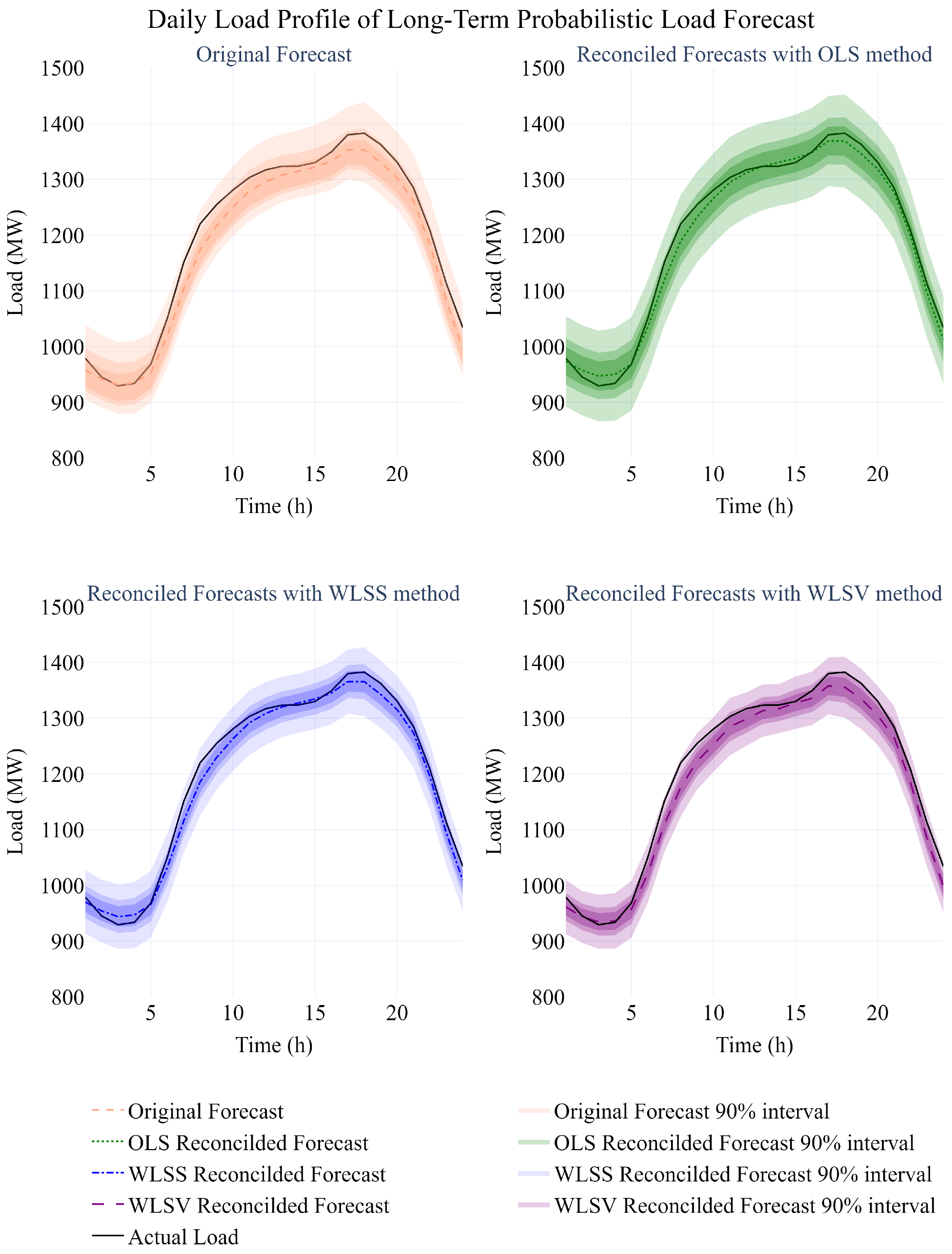
Considering the effectiveness of the optimal reconciliation methods for ex ante long-term probabilistic hourly load forecasts, Figure 4 presents the deterministic and probabilistic averaged daily load profiles extracted from the original forecasts as well as the reconciled forecasts using the OLS, WLS_S, and WLS_V methods for the city of Calgary for the last year of the forecasting horizon.

Generally, the original forecasting model under-forecasts the hourly load, and reconciliation results in increased hourly forecasts. The WLS_S and OLS methods provide deterministic daily load profiles which are very close to the actual averaged daily load profile. The larger area inside the prediction intervals for the OLS method results in higher reliability while lowering the sharpness. However, the positive effect of reliability is bigger than the negative effect of sharpness, which results in better probabilistic scores.

The empirical results demonstrate that reconciliation methods can significantly influence both the accuracy and coherence of long-term load forecasts. In particular, the OLS method consistently improves forecast accuracy in probabilistic settings across all datasets and time resolutions, outperforming WLS_S and WLS_V in most cases. This aligns with findings from [20,27], where OLS reconciliation methods were noted for their stability and simplicity, especially under Gaussian assumptions. However, unlike short-term forecasting contexts in prior studies, the long-horizon and multi-resolution nature of this framework introduces more pronounced variability, especially in ex ante forecasts.

WLS methods rely on assumptions about the underlying error distributions. Our experiments spanning multiple test years and three different regions demonstrate that the reconciliation framework performs consistently well even under moderate violations of these assumptions. The exploration of both in-sample and out-of-sample error-based reconciliation (WLS_V vs. WLS_V-OSE) also provides insight into the tradeoff between theoretical rigor and practical robustness. Further work could explore more flexible nonparametric approaches to estimating the error covariance structure, or could employ resampling techniques to assess the sensitivity of reconciliation outcomes.

Interestingly, WLS_S performed competitively in deterministic forecasting, particularly for hourly and daily forecasts. This suggests that structural scaling, which assumes error consistency within levels, may be better suited to high-resolution load patterns. WLS_V, which is designed for situations where bottom-level variance dominates, showed mixed performance, sometimes worsening aggregated forecasts, especially under out-of-sample error scenarios.

Moreover, differences in reconciliation effectiveness across cities may relate to variations in load composition and demand volatility. Calgary, for example, exhibited stronger improvement under OLS at the daily peak level, potentially due to more predictable consumption patterns compared to the Province-wide Alberta dataset. Overall, these findings underscore that the choice of reconciliation method is not one-size-fits-all. Forecasting context, including resolution, geography, forecast horizon, and data quality, should drive method selection. This flexibility is particularly important in energy systems, where different regions operate under distinct market rules, regulatory environments, and weather-driven variability. These variations indicate that the spatial and temporal granularity of demand data significantly affect reconciliation outcomes, which is another factor warranting further study.

While the proposed method offers significant accuracy gains and coherent forecasts, it assumes that the forecast error distributions are stable and approximately Gaussian, an assumption that may not hold for all regions or forecasting resolutions. Future work should consider non-Gaussian reconciliation strategies and explore hybrid or adaptive methods that respond dynamically to forecast uncertainty structures.

5. Conclusions

In this study, we present a novel approach to long-term electricity load forecasting by integrating temporal hierarchies with advanced reconciliation methods. Our methodology utilizes historical weather data and economic variables to generate probabilistic forecasts at multiple resolutions (hourly, daily, monthly, and yearly) enhancing the reliability and coherence of the predictions.

The results demonstrate the effectiveness of reconciliation methods in improving forecast accuracy. Notably, the OLS method emerges as a standout performer for ex ante probabilistic forecasts, consistently enhancing the Pinball and Winkler scores across all datasets. While the WLS_S shows promise in deterministic forecasts, it did not perform better than the OLS method in probabilistic scenarios.

There was a gap between the performances of different methods in ex post and ex ante forecasting. The introduction of a new source of error by generating input scenarios affected the behavior of different reconciliation methods. The results also indicate that there may be a load composition effect in reconciliation quality. The difference in customer behavior, and consequently in load patterns, introduces a different type of error into the model. Because the error is very important in reconciliation, the effects of customer behavior on load needs to be considered in future works.

The proposed probabilistic multi-resolution long-term forecasting framework provides utilities and system planners with more granular and coherent demand forecasts that can support a range of operational and strategic decisions. For instance, hourly and daily forecasts at the one-year horizon can inform demand response planning, peak load resource scheduling, and seasonal reliability assessments. Probabilistic forecasts made by quantifying forecast uncertainty can enable risk-informed decision-making such as planning based on high-percentile demand scenarios (e.g., P90) rather than single-point estimates. The ability to reconcile forecasts across resolutions further supports consistency in planning activities at both operational and policy-making levels. Our findings underscore the importance of utilizing coherent forecasting approaches that account for the hierarchical nature of electricity demand. Adopting such methods can better inform decision-makers and stakeholders in the energy sector, ultimately leading to more efficient energy management and planning. Future work might explore the integration of this forecasting framework into optimization models for resource allocation, capacity expansion, and regulatory planning under uncertainty.

In conclusion, our work contributes to the growing body of literature on long-term probabilistic electricity load forecasting by demonstrating the utility of temporal hierarchies and reconciliation methods, providing a robust framework for more accurate and coherent load forecasts in the face of an evolving energy landscape.

In future work, we would like to expand the proposed methodology to explore a spatiotemporal hierarchy structure in probabilistic long-term ex ante load forecasting, which would add scalability to the existing model. Forecasting loads for large systems requires a preprocessing step involving fast and global weather station selection and scenario generation.