Artificial Neural Network-Based Mathematical Model of Methanol Steam Reforming on the Anode of Molten Carbonate Fuel Cell Based on Experimental Research

Abstract

The article describes a mathematical model of methanol steam reforming taking place at the anode of a molten carbonate fuel cell (MCFC). An artificial neural network with an appropriate structure was subjected to a learning process on the data obtained during an experiment on the laboratory stand for testing high-temperature fuel cells located at the Institute of Heat Engineering of the Warsaw University of Technology. The backpropagation of error method was used to train the neural network. The training data included the results of methanol steam reforming in the fuel cell for steam-to-carbon ratios of 2:1, 3:1, and 4:1. The artificial neural network was then asked to generate results for other steam-to-carbon ratios. As a result, the artificial neural network predicted that the highest power density for a molten carbonate fuel cell working on methanol would be obtained with a steam-to-carbon ratio of 2.8:1. The article’s key achievement is the application of artificial intelligence to calculate an unusual steam-to-carbon ratio for the methanol steam reforming process occurring directly at the anode of an MCFC fuel cell. The solution proposed in the article contributed to reducing the number of experimental studies.

1. Introduction

Due to the rapid changes in the climate recently [1], the reduction of greenhouse gas emissions into the atmosphere is becoming more and more important [2]. For these reasons, more and more efficient methods of electricity generation and the use of renewable energy, including biofuels [3], are promoted [4], and various policies across the globe are being introduced in order to save the planet [5]. Alcohols such as methanol [6] and ethanol may be an example of such a biofuel as well as e-fuels [7]. If this type of fuel is used in devices for the production of electricity characterized by very high efficiency, such as fuel cells, then the impact of such electricity generation on the environment is even smaller [8]. The state of development of this type of technology is described in this section.

Perez-Trujillo et al. [9] summarize research performed experimentally and numerically in a reversible molten carbonate cell using a single cell with an electrode–electrolyte interface of 80 cm². This was the first time that a molten carbonate single cell has been tested in a reversible mode. The tested cell had an active contact area of 80 cm². The cell electrodes consisted of an alloy of Ni and lithiated NiO, respectively, for the fuel electrode and the oxygen electrode. In this investigation, researchers applied an electrolyte that had an eutectic mixture of 62/38 mol% Li₂CO₃/K₂CO₃. The result of the study was an assessment of the impact of changes in composition, flow, and temperature when the cell was operating in a reversible mode.

The MCFC fuel cell can also be fueled with methane via a dry reforming process (DR-MCFC) [10].

In the following paper, Perez-Trujillo et al. [11] present an isothermal electrochemical model of a MCFC working in a reversible mode. First, the model was equipped with experimental data of a single cell operating in a fuel cell mode only. Then, the model of MCFC was used to calculate the values of overpotentials of the MCFC working as an electrolyzer. The experimental data used in the study came from data published by Perez-Trujillo et al. [9]. Two experimental investigations were performed, where the first one was designed to provide validation data for reported dimensionless models, while the second campaign was designed to provide data about the cell operating in a reversible mode. In the first experimental campaign, the reference condition was the composition of gases at the fuel electrode of 18% CO₂, 11%/H₂O, and 71% of H₂ (with 0% of N₂) at a flow rate of 217 mL/min and in the oxygen electrode of 6% of CO₂, 12% of O₂, and 82% of N₂ at a flow rate of 2566 mL/min and a cell temperature of 650 °C. In the second experimental campaign, focused on studying the reversible effects of MCFCs, a new reference condition was used and more parameters were tested; reference conditions were gas composition at the fuel electrode of 25/25/25/25% of CO₂/H₂O/H₂/N₂ at a flow rate of 330 mL/min and oxidant composition of 25/25/50% of CO₂/O₂/N₂ at a flow rate of 660 mL/min, with a temperature of 650 °C.

In review by Sangarunlet et al. [12], the characteristics and technologies used for the production of MCFCs are presented in a simplified way. The study also includes a financial analysis of a power plant based on MCFC.

The study by Maggio et al. [13] present the possibility of supplying a molten carbonate fuel cell with methanol and ethanol using internal reforming in the cell, enabling flexibility in fuel use, unfeasible for other types of fuel cells operating at lower temperatures.

In the study by Silva et al. [14], the authors conducted a thermodynamic evaluation of the steam reforming of several oxygenated hydrocarbons—including ethanol, glycerol, n-butanol, and methanol—with and without the use of CaO as a CO₂ sorbent, aiming to identify optimal conditions for high-purity hydrogen production. Their findings demonstrate that sorption-enhanced steam reforming (SESR) is a versatile and effective approach for generating hydrogen with minimal concentrations of CO, CO₂, and CH₄ within the 723–873 K temperature range. Moreover, the CO₂ separation rate from the gas phase significantly inhibits carbon deposition at lower temperatures. For all oxygenated hydrocarbons studied in this work, thermodynamic predictions indicate that high-purity hydrogen with a CO content of 20 ppm, required for proton membrane fuel cell (PEMFC) applications, can be directly produced in a single-stage SESR process in the temperature range of 723–773 K at a pressure of 3–5 atm. Thus, further processes involving reactors of the WGS (water–gas shift) type and preferential oxidation of CO (COPrOx) are not necessary.

There are various methods of mathematically describing the operation of fuel cells [15,16], although this article focuses on the use of artificial neural networks for this purpose.

The study by Zhou et al. [17] presents a simple procedure for using machine learning (ML) to diagnose faults in fuel cells. Experiments must be performed in a variety of operational situations, including fault-free states, throughout the data collection phase, and the fault-imposing mechanism must be carefully designed. Then, a diagnostic model based on the ML method is trained and a signal-SoH (State of Health) link is created. Finally, the model can be used to monitor SoH in the cell system. In accordance with the premise of defect detection, diagnostic signals should be as basic as possible.

In a paper by Zhang et al. [18], a deep machine learning technology for simultaneous fault diagnosis of a solid oxide fuel cell system is presented and a novel method of simultaneous fault diagnosis based on a deep learning network called stack autoencoder is proposed.

In the study by Zheng et al. [19], a method for predicting PEMFC (proton-exchange membrane fuel cell) performance using a recurrent neural network (RNN) long short-term memory (LSTM) was proposed. In the paper, the main performance indicators of the PEMFC are the polarization curve and the voltage degradation curve (current-time curve). Both polarization curve prediction and PEMFC performance degradation prediction can be successfully implemented based on the LSTM method. The proposed prediction method is confirmed by PEMFC polarization curve data obtained from the designed aging experiment of a 4 kW stack operating under dynamic load cycles for 600 h.

The article by Gnatowski et al. [20] presents a numerical simulation of transport phenomena inside the anode of a solid oxide fuel cell. The classical mathematical model leads to a significant discrepancy between the measured and predicted voltage values. One possible reason is the assumption of constant values of the charge transfer coefficients in the electrochemical reaction. In the modified formulation of the problem, the correction of the charge transfer coefficients in the model of the electrochemical reaction was taken into account. A dedicated calculation scheme is presented in which the artificial neural network updates the charge transfer coefficients depending on the operating conditions and available data sets. The neural network was trained on twelve experimental anode polarization curve data points obtained from literature. The training set included data for an anode operating at two different temperatures: 800 °C and 900 °C. The test set additionally included six data points for the anode operating at 1000 °C.

In the study by Nassef et al. [21], a modern optimization algorithm was built to maximize the efficiency of a solid oxide fuel cell. First, the cell is modeled using artificial neural networks based on experimental data sets. Then, a robust, simple, and fast optimization algorithm called radial movement optimizer is used to determine the cell’s optimal operating parameters. The cell parameters used in the optimization process are the thickness of the anode support layer, anode porosity, electrolyte thickness, and the thickness of the cathode interlayer. The obtained optimization results are compared with the previous, optimized experimental results and results obtained using the genetic algorithm.

In research reported by Wilberforce et al. [22], the use of an artificial neutral network (ANN) for determining the voltage and current obtained from a fuel cell with a proton exchange membrane of the area of 11.46 cm² was investigated. Performance predictions for group method of data handling (GMDH) as well as feed forward back propagation (FFBP) neutral networks were used to estimate the current and voltage obtained from the proton exchange membrane fuel cell under study. The study presented models with good predictions, although the GMDH neural network performed better than the FFBP neural network. The study therefore proposed the GMDH neural network as the best model to predict the performance of a proton exchange membrane fuel cell.

Molten carbonate fuel cell (MCFC) models based on artificial neural networks and their learning processes were the subject of the article by Milewski et al. [23]. The proposed models were designed to simulate the operation of the cell depending on various parameters, starting from a simple model taking into account only the influence of temperature and ending with a complex model with 14 inputs (corresponding to 14 parameters). The artificial neural networks used consisted of three layers: input, hidden (consisting of three neurons), and output. The activation functions for the hidden layer and the output layer were hyperbolic tangent and linear function, respectively. Various network configurations were tested. The average error of mapping the cell behavior by the ANN models used ranged from 2.4% to 4.6%.

The use of artificial neural networks to model the steam methane reforming process itself is presented in [24]. In the review shown above, we can find the use of artificial neural networks to model the performance of fuel cells (including MCFCs), but not those powered with the use of the internal steam reforming process.

Accurate modeling of fuel cell processes is crucial for design optimization and control. Classical modeling approaches for fuel cells are physics-based models that range from 0D lumped parameter formulations to multi-dimensional CFD simulations. These models explicitly incorporate underlying transport and electrochemical phenomena—for example, MCFC models include detailed equations for electrochemistry, heat transfer, gas diffusion, and even intrapore mass transport within porous electrodes [23].

Such mechanistic models provide high physical fidelity and insight: they can capture temperature gradients, concentration distributions, and reaction kinetics across the cell with rigorous adherence to physical laws. Similar multi-physics modeling frameworks exist for proton-exchange membrane fuel cells and solid oxide fuel cells, which account for phenomena like water management or internal reforming with comparable detail [25]. The trade-off is that increased physical fidelity comes with greater complexity and computational cost. High-dimensional models (e.g., 2D/3D CFD) resolve fine spatial details of flow, heat, and species profiles but require significant computation time and input of many parameters. Even reduced-order or 1D models often involve coupled nonlinear equations that can be time-consuming to solve [26].

In contrast, data-driven approaches such as ANNs have emerged as efficient modeling tools in fuel cell research. ANNs forego explicit physics and instead learn the relationship between inputs and outputs by training on data. In essence, an ANN acts as a nonlinear regression model that can approximate the fuel cell’s internal functional mapping without detailed knowledge of the physics [27]. For example, an ANN can be trained to predict a cell’s voltage or efficiency given conditions like current density, gas flow rates, and temperatures—effectively modeling the process within the cell by learning from empirical or simulated data. Once trained, the network yields an instantaneous prediction for any new input conditions. Studies have shown that relatively simple ANN architectures can accurately reproduce fuel cell performance; for instance, a multilayer ANN taught on limited data from a validated physical model could predict MCFC (and other fuel cell types) operating parameters (voltage, flow rates, etc.) with average errors below 1% [28]. ANNs excel at capturing complex, nonlinear interactions among variables and can generalize from the trends in the training data. Moreover, their computational overhead at runtime is minimal—a feed-forward calculation is essentially just algebra, making ANNs well-suited for real-time applications and extensive parametric analyses.

However, the advantages of ANNs come with important trade-offs. A primary critique is that pure ANN models “hide the physics” of the process: they function as black boxes with no transparent connection to physical laws. Unlike a mechanistic model, which can provide insight into internal states (e.g., temperature profiles or species distributions) and ensures consistency with conservation principles, an ANN offers little interpretability of its internal parameters (weights) in physical terms. This lack of physical interpretability can be a drawback when understanding failure modes or extrapolating beyond the training regime. Furthermore, ANN-based models are data-dependent—their accuracy and scope are limited to scenarios represented in the training data. They may perform interpolations with high accuracy but their predictions become unreliable if asked to extrapolate to novel conditions outside the data range. In contrast, a well-formulated mechanistic model, grounded in first principles, can often be more confidently applied to new scenarios (assuming the underlying physics remain unchanged). Finally, developing an ANN model requires a sufficiently large and representative dataset (either from experiments or high-fidelity simulations), and training the network involves its own offline computational cost. These considerations illustrate a fundamental trade-off between classical and ANN-based modeling: the former offers physical transparency and potentially broader validity at the expense of computational intensity, while the latter provides rapid, flexible predictive power at the expense of direct physical insight and strict reliance on data.

Table 1. Comparison of classical models vs. ANN-based models for fuel cell simulation.

Feature	Classical Models	ANN-Based Model
Physical interpretability	High—built on physical laws; model parameters and internal states have direct physical meaning (e.g., concentrations, temperatures), aiding insight and diagnosis.	Low—treated as a “black-box” function approximator with no explicit physics; internal weights are not readily interpretable in physical terms.
Physical fidelity	High—can include detailed multiphysics (electrochemistry, thermal effects, mass transport, intrapore diffusion, etc.) for accurate cell behavior. Valid over wide range if physics captured.	Variable—captures the observed input–output behavior (including nonlinear couplings) within the domain of training data. Does not inherently enforce physical laws or constraints (risks unphysical predictions if extrapolated).
Computational cost	High—solving coupled ODE/PDE systems (especially in 2D or 3D CFD models) is computationally intensive. Simplified 0D/1D models are faster but can still be too slow for real-time control in complex cases.	Low (for inference)—once trained, ANN evaluation is almost instantaneous (matrix operations), enabling real-time predictions and fast simulations. Training the ANN can be time-consuming but is performed offline.
Data requirements	Low–Moderate—primarily requires physical properties and some experimental calibration. Mechanistic models extrapolate based on physics, so extensive operational datasets are not strictly necessary (though they improve parameter tuning).	High—requires a large, representative dataset to train the model. Model accuracy and scope depend entirely on the quality and breadth of training data; capturing all relevant operating conditions in the dataset is crucial.
Predictive accuracy	High (within model validity)—can predict performance trends reliably if all key physics are included. Errors mainly arise from uncertain parameters or neglected phenomena.	High (within training domain)—can achieve very low error on test data in the range of training (e.g., <1% in voltage prediction). But accuracy degrades outside the trained domain, where predictions can become unreliable.
Typical use cases	Detailed design and analysis; performance prediction with insight into internal behavior; virtual prototyping and optimization studies; model-based control (using reduced models). Widely used in research and engineering to evaluate effects of design changes or to investigate phenomena (e.g., water management in PEMFC).	Surrogate modeling to replace expensive simulations (e.g., in optimization or real-time system simulation); control system models for observers or controllers; fault diagnosis and prognostics (pattern recognition). Chosen when rapid output is needed or when the process is too complex for explicit modeling, provided sufficient data is available.

summarizes the key differences between traditional fuel cell models and ANN-based models, highlighting their features, strengths, and limitations in the context of fuel cell simulations.

This article describes the use of artificial neural networks to predict the performance of an MCFC fuel cell fueled with a mixture of methanol and steam (as a result of an internal steam reforming process) in various steam-to-carbon ratios, which distinguishes it from previous studies. It is important because such tests require prior preparation of a mixture of methanol and water in the appropriate proportion. Thanks to this, it was possible to perform fewer tests to achieve this goal.

Research on MCFC cells has gained popularity recently, and the application of synthetic fuels (which methanol is ) is even more important at this moment, as methanol is the most basic and easiest to synthesize synthetic fuel. What’s more, MCFC can be applied to produce synthetic gas in order to produce methanol (when working in the co-electrolysis mode), thus generating a form of power-to-liquid or power-to-gas energy storage unit.

Having experience in the application of ANN models to MCFC modelling [23], we decided that the steam-to-carbon ratio could be optimized via artificial neural network, combining two most important aspects of MCFCs, partial pressures and steam reforming kinetics, without going deeply into those processes, which are very complicated but can be addressed and optimized by ANN thought on experimental data.

It should also be emphasized that there are no reports showing the results of modelling MCFC fuel cells fueled with synthetic fuels such as methanol using artificial neural networks. Therefore, this article addresses this knowledge gap. Such studies have so far been carried out for other types of fuel cells (SOFCs and DMFC proton cells) but not for MCFC fuel cells. Recently, an article showing utilization of ammonia in MCFC was presented [29] concerning a similar subject, though utilizing a different fuel.

2. Materials and Methods

The modelling approach chosen for the research is based on our previous works where we demonstrated that MCFC can be fueled with various fuels including liquid fuels such as alcohols [30] with various steam-to-carbon ratios, and it can operate without negative impact on the fuel cell anode [31]. Investigations shows, however, that the steam-to-carbon ratio is very important as the MCFC operates based on partial pressure differences, and when it comes to the steam reforming process, the kinetics of reaction plays a main role [32].

2.1. Steam Reforming

Hydrogen can be produced at the anode of MCFC from methanol by its decomposition, steam reforming, and conversion of carbon monoxide with steam (WGS—water–gas shift), as shown in Equations (1)–(3).

Methanol decomposition is shown using Equation (1).

$$C{H}_{3}OH \to 2H_2+CO\hspace{1em}[∆H=+90.2 \mathrm{k}\mathrm{J}/\mathrm{m}\mathrm{o}\mathrm{l}]$$

(1)

Steam reforming of methanol can be described by Equation (2).

$$C{H}_{3}OH+H_{2}O \to 3H_2+C{O}_2\hspace{1em}[\Delta H=+49.7 \mathrm{k}\mathrm{J}/\mathrm{m}\mathrm{o}\mathrm{l}]$$

(2)

In turn, the water–gas shift reaction is represented by Equation (3).

$$CO+H_{2}O\to C{O}_2+H_2\hspace{1em}[\Delta H=-41 \mathrm{k}\mathrm{J}/\mathrm{m}\mathrm{o}\mathrm{l}]$$

(3)

Methanol steam reforming is a mature and extensively studied process, established over the past two to three decades [33]. It is commonly conducted at atmospheric pressure within a temperature range of 200–300 °C, utilizing copper-based catalysts such as Cu-ZnO-Al₂O₃ or noble metal-supported systems.

The important issue regarding the anode of the molten carbonate fuel cell is that it is commonly made of nickel, which is also a desired material serving as a catalyst in the methanol steam reforming process.

Utilizing hydrocarbon-based fuels can cause solid carbon deposition on the catalyst surface. Preventing such behavior can be achieved by raising the temperature or/and introducing water molecules into the stream. The amount of water is defined by the ratio between water and carbon content at the inlet of the reaction, called the steam-to-carbon ratio, s/c. Typically, an S/C ratio between 1 and 2 is used. A higher S/C ratio may favor WGS, which may reduce the concentration of carbon monoxide in the product stream and may also help suppress carbon deposition on the catalyst surface.

A comparison of different mathematical models describing the steam reforming process in a classical way was presented in the authors’ earlier work [32].

2.2. MCFC

A molten carbonate fuel cell (MCFC) is a high-temperature type of fuel cell that uses an electrolyte in the form of molten carbonates. To melt the electrolyte, the fuel cell operating temperature should be above 500 °C. The typical operating temperature of an MCFC is about 650 °C.

The cell configuration typically includes a porous nickel anode, lithiated NiO cathode, and an electrolyte consisting of a mixture of Li₂CO₃ + K₂CO₃ (lithium and potassium carbonates, 62% and 38 mol%, respectively), which will impregnate the supporting ceramic matrix made of lithium aluminate (LiAlO₂). The MCFC operation involves a series of electrochemical reactions occurring at the electrodes and electrolyte interface—details are described by Vielstich [34].

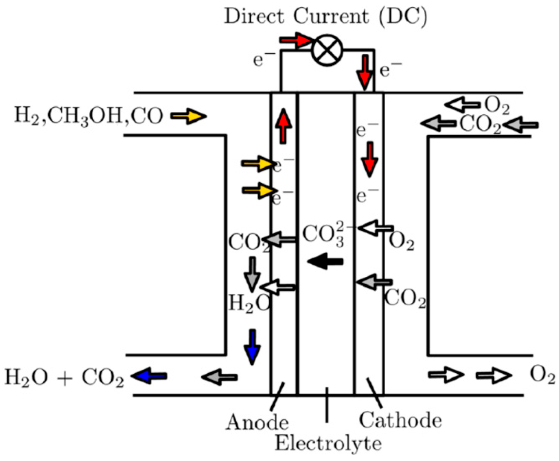
On the cathode side, air or oxygen together with carbon dioxide are supplied, reacting with the electrolyte to form carbonate ions $C{O}_2^{=}$ (cathode reaction, Equation (5)). These carbonate ions then migrate to the anode side (Figure 1), where hydrogen is supplied and reacts with carbonate ions to produce water and carbon dioxide (anode reaction, Equation (4)). The flow of electrons through the external circuit generates electricity. As a by-product of the overall reaction (Equation (6)), water and heat are produced.

$$H_2+C{O}_2^{=}\to H_{2}O+C{O}_2+2e^{-}$$

(4)

$${\displaystyle \frac{1}{2}}{O}_2+C{O}_2+2e^{-}\to C{O}_3^{=}$$

(5)

$$H_2+{\displaystyle \frac{1}{2}}{O}_2\to H_{2}O+Heat [\Delta H=-242 \mathrm{kJ}/\mathrm{mol}]$$

(6)

Overall, modeling of the MCFC can be carried out in many ways [35,36,37,38,39]. One of the most feasible and well-proven methods is described in a paper by Milewski et al. [40]. This model is a 0D mathematical model that is reliable and can be used both in simulation and optimization of MCFC and has been proven to be functional even for dynamic simulations of MCFC.

However, in this paper, the modeling will be realized based on the artificial neural networks that will be described in the next subsection.

The main parameters of the components of the tested MCFC fuel cell are presented in

Table 2. The construction parameters of the tested MCFC elements.

Element	Dimensions	Material	Porosity	Thickness
Fuel electrode	50 × 50 mm	Ni	55%	0.65 mm
Oxidant electrode	45 × 45 mm	NiO	78%	0.65 mm
Matrix	70 × 70 mm	γ-LiAlO2	40%	0.3 mm
Electrolyte	2.15 g	Li2CO3/K2CO3, 62/38	-	-

. The fuel electrode was based on nickel sinters that are characterized by 55% open porosity with thickness of 0.65 mm, while the oxide electrode was made of nickel oxide with the same thickness and structure. The electrolyte was composed of potassium carbonate and lithium carbonate with a molar ratio of 38/62 and a total mass of 2.15 g. The polymer-based slurry with ceramic powder was tape-cast to create a matrix. The foundation powder was LiAlO₂, while the slurry contained chemicals that were removed during the first fuel cell start-up procedure. The homogenization of the slurries was conducted using a THINKY ARV-930TWIN planetary centrifugal vacuum mixer to ensure uniform dispersion of the components. The slurries were cast onto a polymer substrate and dried at room temperature for 24 h to form green tapes, which were then prepared for cell assembly.

The cell was positioned between two current collectors that were manufactured from stainless steel 310SS and had an active area that was predicted to be 20.25 cm² (measured as the size of cathode, which was 4.5 cm × 4.5 cm). The current collectors were fitted with passageways that allowed fuel and oxidant flows to pass through them.

2.3. Artificial Neural Networks

Artificial neural networks emulate networks based on neurons. Neurons receive information via dendrites, process it via the nucleus and activation function, and convey output through synapses and the axon. Artificial neural networks use activation functions such as sigmoid, hyperbolic tangent (tanh), or ReLU, with nonlinear functions being predominant owing to their capacity to accommodate many input sources. The input of each node has a weight that is modified throughout training, and the output is determined by summation and activation functions (e.g., tanh). An ANN node needs an activation (or logistic) function. It evaluates node output as “yes” or “no”. Mathematically, the resultant value can be 0; 1, −1; 1, etc. Sigmoid, hyperbolic tangent, and rectified linear unit functions are the most popular activation functions. Linear and nonlinear activation functions exist. Nonlinear functions are most common because they can handle more data types. Most activation functions forecast probability using the sigmoid function (Equation (7)).

$$\sigma (x)={\displaystyle \frac{1}{1+e^x}}$$

(7)

In each node, the input variables have their own weight (w_k;i;j) adjusted in the training process. The products of input variables and weights are grouped into the summation part (s_k;i, Equation (8)). The activation function used in this article is tanh, and it cooperates with summation according to Equation (9).

$$s_{k,i}=\sum _{j=0}^{N_{k-1}} w_{k,i,j}\cdot x_{k,j}$$

(8)

$${\sigma }_{k,i}={\displaystyle \frac{1-e^{-2s_{k,i}}}{1+e^{-2s_{k,i}}}}$$

(9)

The Mean Square Error function reduces mistakes throughout the training process. Forward differentiation propagates data across layers, while backward differentiation, or backpropagation, modifies weights.

$$E_{MSE}={\displaystyle \frac{1}{2}}\sum _{p=1}^P \sum _{m=1}^M e_{p,m}^2$$

(10)

Forward and backward differentiations are employed by ANNs. In ANNs, input, hidden, and output layers exist. From the input layer to the output layer, forward differentiation is iterated. In reverse, iterations begin at the output layer and record the values of each layer. Backward differentiation, also known as automated differentiation, is the optimal method for the majority of ANNs. Backpropagation (BP), a backward differentiation-based ANN training technique, was employed to represent MCFC. Backpropagation (BP), a backward differentiation-based ANN training technique, was employed to represent MCFC.

The Levenberd–Marquardt (LM) algorithm was utilized to minimize nonlinear functions throughout the training procedure (Equation (11)) [41]. Levenberg and Marquardt developed the algorithm to solve nonlinear least-squares problems. The LM algorithm is a synthesis of the Gauss–Newton and Steepest Descent training procedures, providing a combined training procedure. It is highly stable and has a rapid calculating speed.

$$w_{k+1}=w_k-{\left(J^{T}J+\mu I\right)}^{-1}{J}_k{e}_k$$

(11)

where e—error vector, J—Jacobian matrix, w—weights of connections between neurons in an artificial neural network, μ—combination coefficient, and I—identity matrix.

The LM algorithm is based on solving the Jacobi matrix. It is introduced because calculation of the second-order derivatives of the error function in a simple way is a very costly computational process. Introducing the Jacobian matrix form (Equation (12)) strongly simplifies the process.

$$\mathit{J}=\left[\begin{array}{cccc}{\displaystyle \frac{\partial e_{\mathrm{1,1}}}{\partial w_1}}& {\displaystyle \frac{\partial e_{\mathrm{1,1}}}{\partial w_2}}& \dots & {\displaystyle \frac{\partial e_{\mathrm{1,1}}}{\partial w_N}}\\ {\displaystyle \frac{\partial e_{\mathrm{1,2}}}{\partial w_1}}& {\displaystyle \frac{\partial e_{\mathrm{1,2}}}{\partial w_2}}& \dots & {\displaystyle \frac{\partial e_{\mathrm{1,2}}}{\partial w_N}}\\ \dots & \dots & \dots & \dots \\ {\displaystyle \frac{\partial e_{1,M}}{\partial w_1}}& {\displaystyle \frac{\partial e_{1,M}}{\partial w_2}}& \dots & {\displaystyle \frac{\partial e_{1,M}}{\partial w_N}}\\ \dots & \dots & \dots & \dots \\ {\displaystyle \frac{\partial e_{P,1}}{\partial w_1}}& {\displaystyle \frac{\partial e_{p,1}}{\partial w_2}}& \dots & {\displaystyle \frac{\partial e_{P,1}}{\partial w_N}}\\ {\displaystyle \frac{\partial e_{p,2}}{\partial w_1}}& {\displaystyle \frac{\partial e_{P,2}}{\partial w_2}}& \dots & {\displaystyle \frac{\partial e_{p,2}}{\partial w_N}}\\ \dots & \dots & \dots & \dots \\ {\displaystyle \frac{\partial e_{P,M}}{\partial w_1}}& {\displaystyle \frac{\partial e_{P,M}}{\partial w_2}}& \dots & {\displaystyle \frac{\partial e_{P,M}}{\partial w_N}}\end{array}\right]$$

(12)

Backpropagation with Bayesian Regularization (also known as BR) was used as the training algorithm. The weights are adjusted accordingly, considering the LM solution. The strategy is highly effective in avoiding both overtraining and overfitting because it treats the weights as random variables and modifies them in accordance with Bayes’ rule (Equation (13)).

$$P(\mathrm{w}\mid D,\alpha ,\beta ,M)={\displaystyle \frac{P(D\mid \mathrm{w},\beta ,M)P(\mathrm{w}\mid \alpha ,M)}{P(D\mid \alpha ,\beta ,M)}}$$

(13)

In this article, the Python 3.12 programming language is used to model artificial neural networks. Based on the results from the neural network, tests were carried out on a fuel cell with the obtained optimal mixture proportions in order to verify the results obtained from the neural network.

2.4. Experimental Setup

Experimental data used for the ANN training purpose were obtained from experimental studies with various mixtures of water/methanol. The active cell area was 20.25 cm² and dimensions are 4.5 × 4.5 cm². Tests were conducted at fuel cell laboratory, which enables examination of MCFC at temperature up to 700 °C. The tests in this article were carried out at the usual operating temperature of MCFC, which is 650 °C. The temperature was maintained at a constant level (650 °C) by electric heaters that were installed in the test stand. The experiments were conducted at atmospheric pressure. The entire test procedure took 4 h in total (excluding the start-up and shutdown of the cell, which took several days).

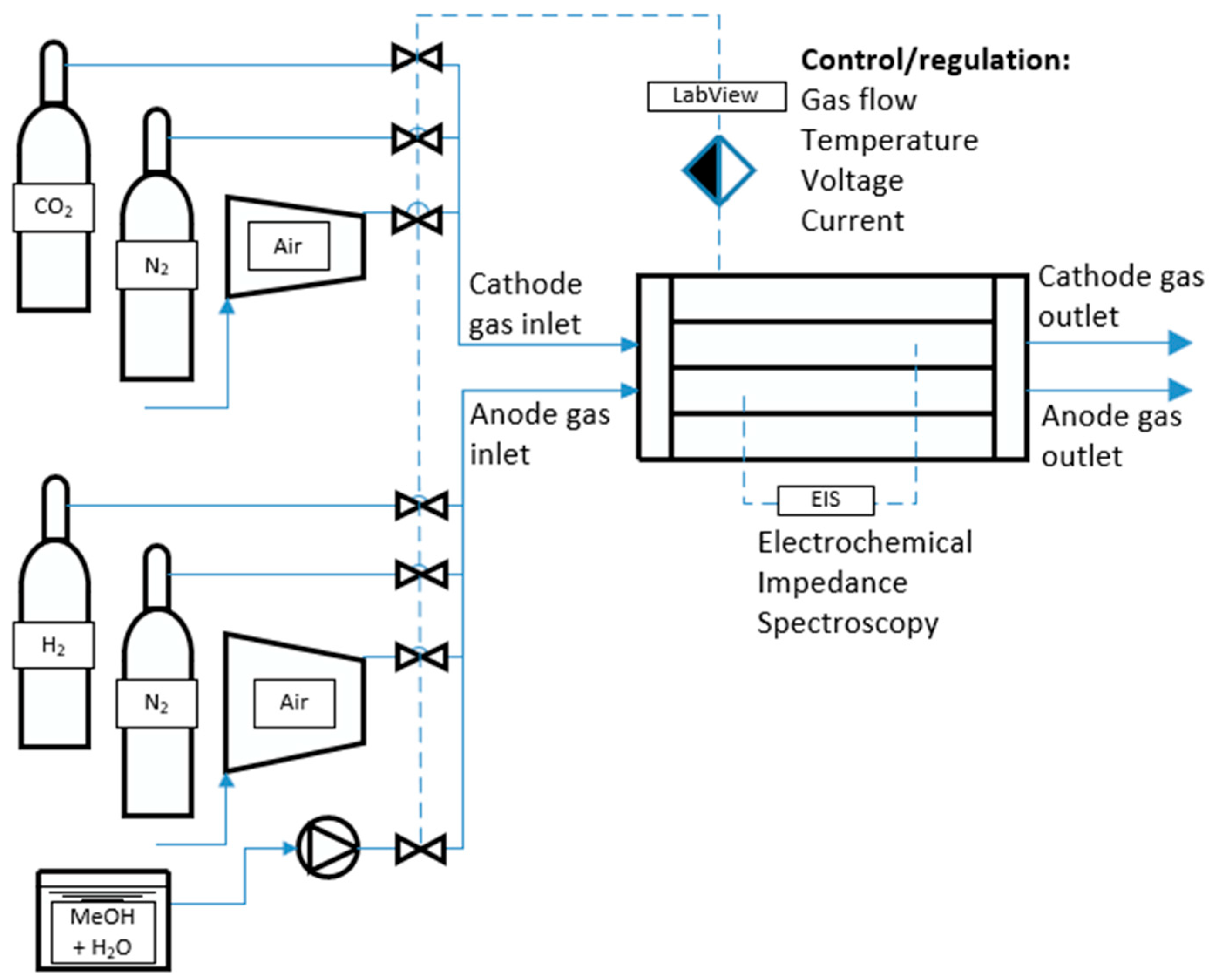
The experimental station comprises a vessel containing a cell-support structure integrated with ancillary instrumentation. It features dual-zone heating, with independent heaters positioned above and below the test cell. Temperature monitoring and regulation are achieved through multiple thermocouples strategically placed across the cell. Feedstock flow rates are precisely managed using Bronkhorst mass flow controllers in conjunction with a Lead Fluid BT100S peristaltic pump. Electrical input and load conditions are governed by a KORAD KD3005P DC linear power supply and an AIM-TTI LD400P electronic load, respectively. To enable testing liquid fuels, the test stand was additionally equipped with a peristaltic pump to deliver fuel directly to the anode channel of the fuel cell. Due to the formation of carbon monoxide as a by-product of steam reforming of alcohols, and because the vapors of the fuels selected for testing can be toxic in high concentrations, the test stand was additionally equipped with a duct fan with sleeves that exhausts the fumes directly outside the laboratory. The liquid fuel is fed directly into the anode channel by means of a peristaltic pump with adjustable flow rate. The photos below show the actual test unit after installation.

The scheme of the experimental stand for testing high-temperature fuel cells at the Institute of Heat Engineering of the Warsaw University of Technology is shown in Figure 2.

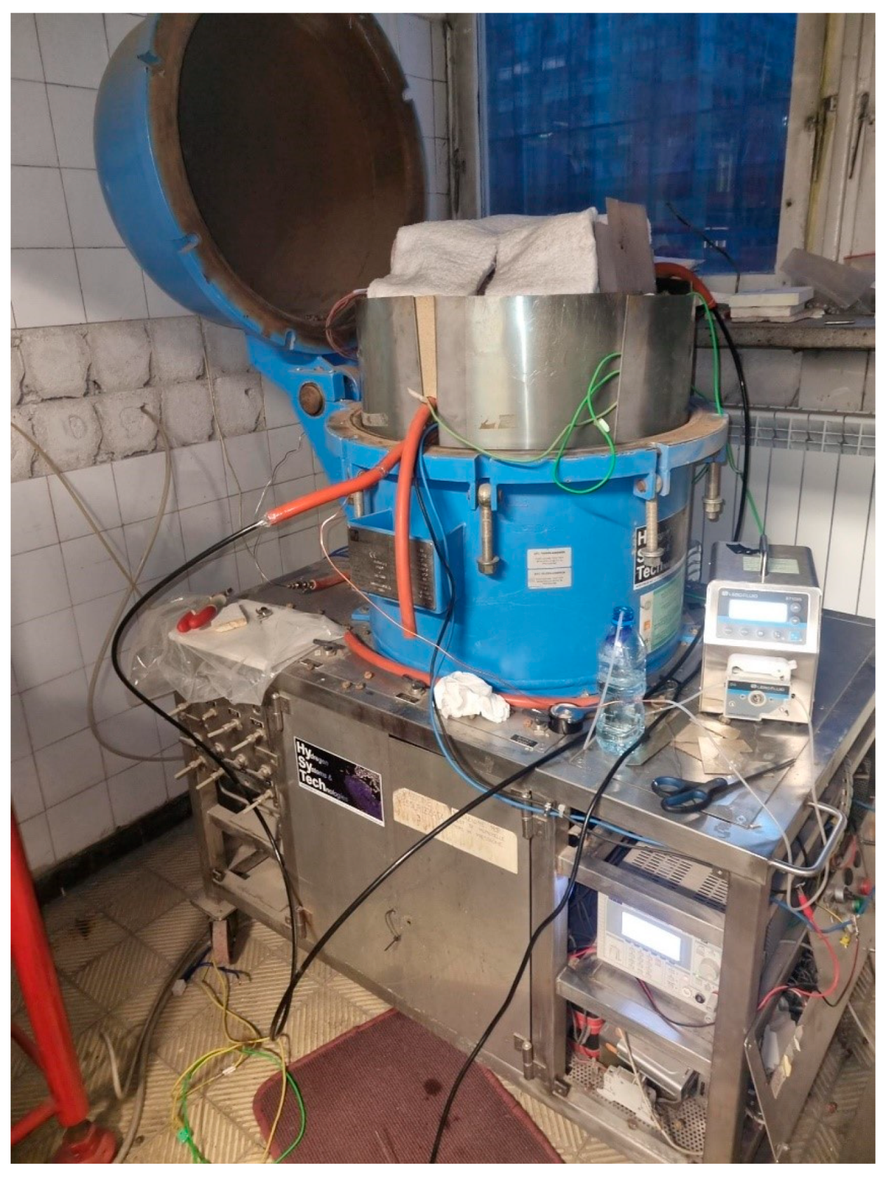
In turn, Figure 3 shows the physical implementation of this experimental stand.

To enable testing liquid fuels, the test stand was additionally equipped with a peristaltic pump to deliver fuel directly to the anode channel of the fuel cell. The liquid fuel, in the form of a ready mixture of water and the test chemical of a certain concentration, is fed directly into the anode channel by means of a peristaltic pump with adjustable flow rate.

3. Results and Discussion

The designed artificial neural network was used for prediction of steam-to-carbon ratio of methanol and water allowing for the best performance of molten carbonate fuel cell powered with liquid fuel mixture.

The input data for building the neural network is the measurement data from the test bench:

-

S/C (steam-to-carbon ratio)—mixture ratio feeding the fuel cell;

-

ICELL—current flowing through the cell;

-

VCELL—cell voltage;

-

P—power of the cell—product of ICELL and VCELL.

For the neural network input, three fuel cell tests were carried out for S/C ratios of 4:1, 3:1, and 2:1 with double cycling, resulting in two current-voltage curves for each fuel mixture, each current–voltage curve containing at least 150 measurement points, giving more than 1200 input points in total. The amount of methanol delivered to the anode side was constant; the S/C ratio was increased by increasing the amount of water (

Table 3. Composition of fuels delivered to the anode side during experiments.

	Mass Flow to the Anode Side (g/h)
Experiment	H2O	CH3OH	Expected Flow of H2 as a Reforming Product (If Steam Reforming Process Was Ideal)
S/C = 4.0	10.69	4.75	0.899
S/C = 3.0	8.02	4.75	0.899
S/C = 2.0	5.34	4.75	0.899
S/C = 2.8	7.48	4.75	0.449

).

The following graphs show the current–voltage curves for each test and plot the power versus current flowing through the cell.

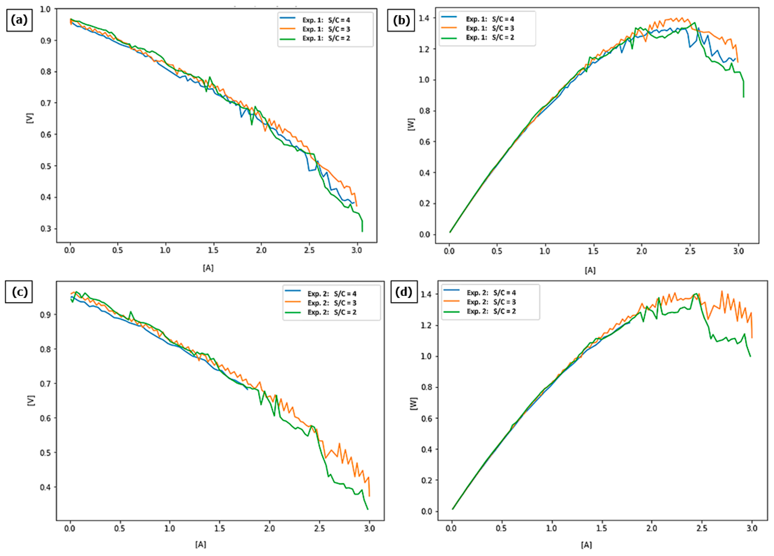
The first experiment delivered current–voltage curves (Figure 4a) in a whole spectrum ranging from 0.4 V to almost 1 V. At higher voltages (lower current), the steam-to-carbon ratio of 2:1 seems to show slightly better results, while at lower voltages and higher current, a steam-to-carbon ratio of 3 is more likely to deliver higher power.

Results observed on the power curve (Figure 4b) show that at the lower current, the difference between various s/c ratios does not impact results much; however, at higher currents, where more of the power can be delivered, an s/c of 3:1 shows the best results.

In the second experiment (Figure 4c), the results were quite similar, as again at higher voltages, an s/c ratio of 2:1 seems to show slightly better results, while at lower voltages, a higher s/c ratio of 3 delivers higher power, while an s/c of 4 did not work at all.

Again, analysis of the power curve for the experiment 2 (Figure 4d) shows that the fuel cell working on an s/c of 3 shows the best results in the area of parameters, whereby the highest power can be obtained from the fuel cell.

Table 4. Achievable maximum powers by the cell in each test.

Fuel Mixture	Experiment Name	Maximum Power Achieved [W]
S/C = 4	experiment 1	1.334
	experiment 2	1.213 *
S/C = 3	experiment 1	1.399
	experiment 2	1.418
S/C = 2	experiment 1	1.368
	experiment 2	1.402

* experiment interrupted.

shows the achievable maximum powers by the cell in each test.

The experimental setup allows us to measure, record, and set the following data: liquid fuel mixture flow (pre-mixed water with methanol, supplied by a capillary tube that terminated in a hot zone of CF allowing for evaporation of the mixture at its end) delivered with variable-speed-drive peristaltic pump, gas flows (hydrogen, CO₂, nitrogen and air) delivered with Bronkhorst gas flow controllers, temperature of anode electrode, temperature of cathode electrode, temperatures of electrodes electric heaters (for temperature stabilization), voltage measured between anode and cathode manifolds, and the current load. The different fuel mixtures were delivered to the fuel cell from outside containers (bottles of pre-mixed water and methanol). All the parameters were registered in more than 1200 points (exactly 365 measurement points for 4:1 ratio, 478 measurement points for 3:1 ratio, 490 measurement points for 2:1 ratio), which were used for ANN modelling.

The following parameters were used in the neural network model using the MLP Regressor class:

• n_layers = 2—number of hidden layers;
• hidden_layer_sizes = 50—number of neurons in hidden layers;
• activation = ‘tanh’—rectified linear unit function, returns f(x) = max(0, x);
• solver = ‘lbfgs’—the limited-memory Broyden–Fletcher–Goldfarb–Shanno (LBFGS) optimization algorithm was used as the solver.

The given structure of the neural network was selected through an optimization process aiming to achieve the smallest mean error of result prediction. The smallest mean error was achieved for the structure consisted of 2 hidden layers with 50 neurons each. More advanced structures do not give performance benefits for the given set of data and expected result but do, however, make the training and prediction processes more resource-consuming.

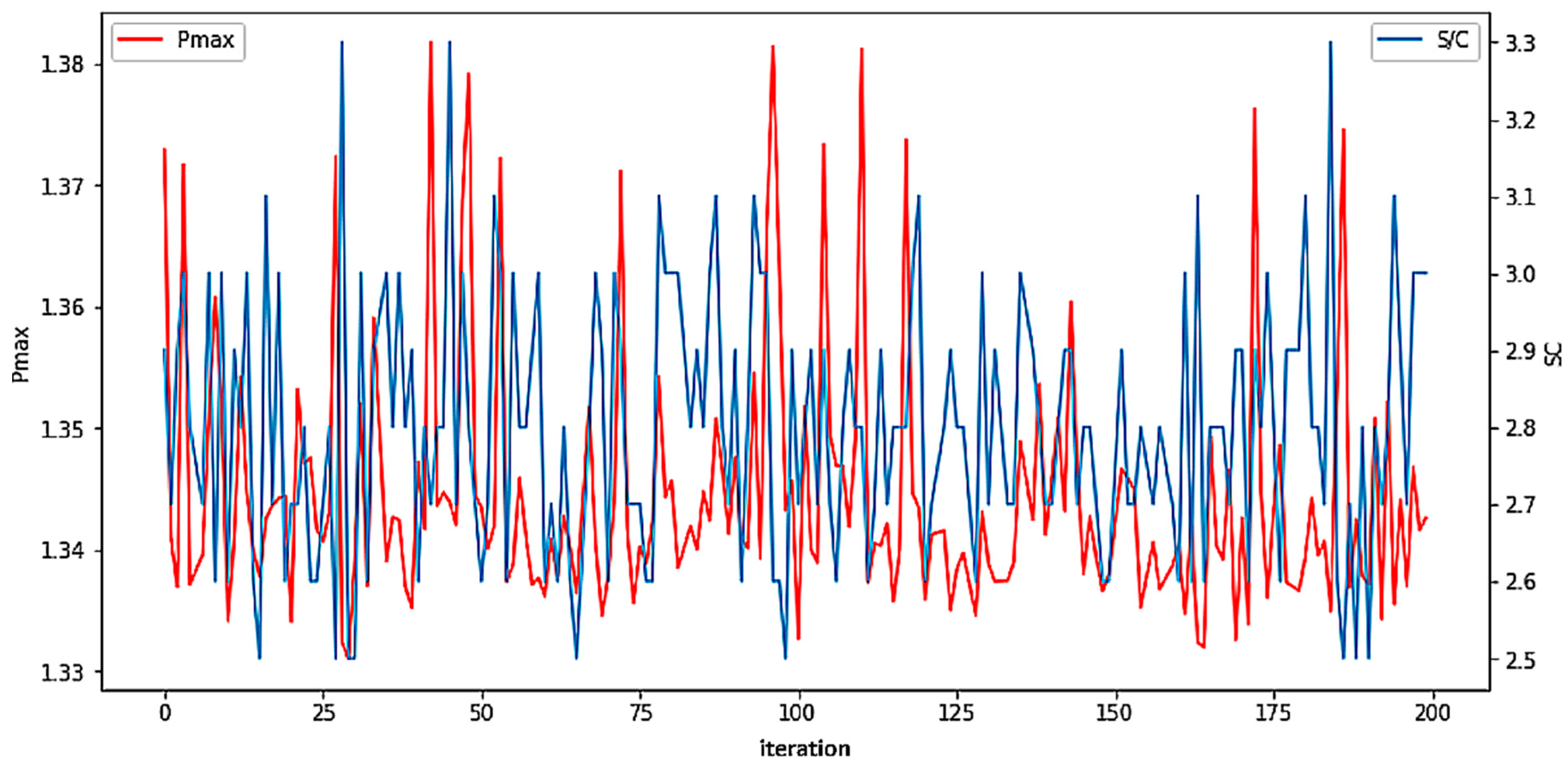
The first iterations were performed to analyze the precision of the model in reflecting the investigated steam/carbon ratios. The neural network model predicts the operating variables of the cell with high accuracy, so it can be used to make predictions for unknown S/C parameters. The diagram below shows the results of 200 iterations of initialization and computation of the neural network.

Figure 5 presents the results of S/C ratio and maximum achieved modeled Pmax within 200 iterations, which were the basis of the final optimum S/C ratio determination. The Pmax varies between 1.33 and 1.38 W, while S/C varies between ratios of 2.5 and 3.3.

The results of the neural network optimization after 200 iterations are shown in

Table 5. Neural network model results after 200 iterations.

Parameter	Result
Average S/C	2.799
Median S/C	2.8
Standard deviation S/C	0.17
Average maximum power	1.344
Median maximum power	1.342
Standard deviation of maximum power	0.01

.

The S/C parameter for which the cell should achieve maximum power is 2.8. As a check, a fuel mixture with a parameter of 2.8 was prepared, then a test was carried out on the cell with the prepared fuel.

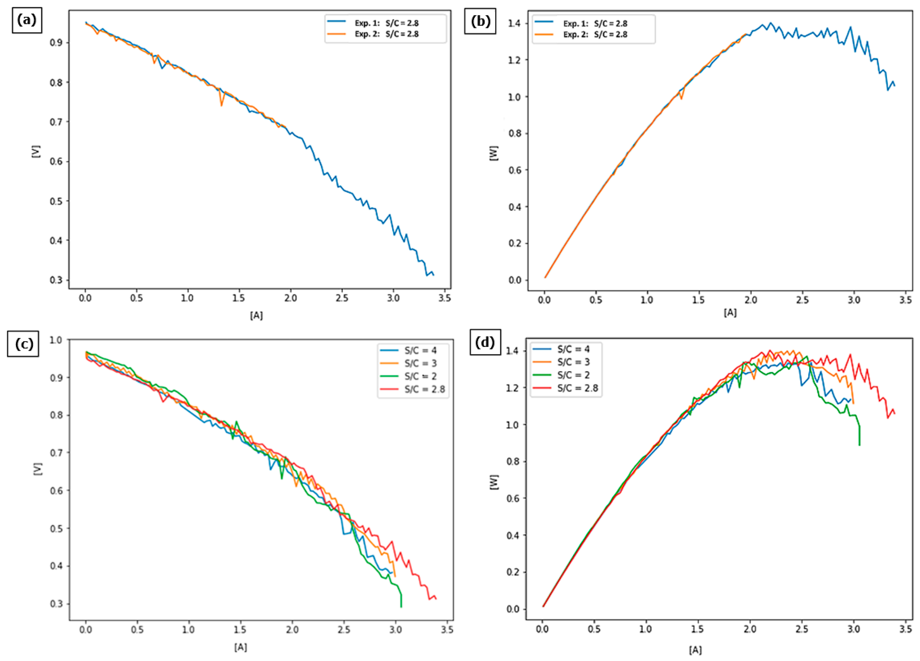
The results (Figure 6a) show that fuel cells could operate in the voltages between 0.3 and almost 1.0 V, reaching a maximum current of almost 3.5 A. The results of two experiments are almost identical in the area where both current–voltage curves could be obtained.

The obtained power curve (Figure 6b) of the optimized S/C ratio fuel shows an unexpected flattening of characteristics in the area where it is supposed to deliver the highest power.

The obtained results were compared to results obtained on three basic S/C ratios.

A comparison of current–voltage curves for all four experiments (Figure 6c) shows that their characteristics are quite similar, while the optimized S/C ratio of 2.8 seems to give the best results when it comes to the maximum current reached by the fuel cell.

The tested cell achieves similar maximum powers for the S/C parameter in the range from 2 to 4, as shown in

Table 6. Comparison of results obtained on the ANN defined S/C between standard S/C ratios.

Fuel Mixture	Maximum Power [W]	Difference Between S/C = 2.8 and Standard S/C
S/C = 4	1.334	−4.78%
S/C = 3	1.418	1.21%
S/C = 2	1.402	0.07%
S/C = 2.8	1.401	-

and Figure 6d. The greatest advantage of the S/C = 2.8 parameter over the other tests is seen in the current-–voltage curves plot, where, in the range above 2.5 A, the cell achieves higher voltage values compared to the other ratios.

From the results obtained, it can be concluded that the neural network used is sufficient to optimize the cell in terms of the S/C parameter. Although the maximum power obtained is not the highest of the tests carried out, it is possible to see an improvement in the cell parameters in the range of high current densities. Improving fuel cell operation in a higher range of current densities may improve the life expectancy of the fuel cells, as the degradation of fuel cells in this range is often much higher and usually leads to a rapid breakdown of the fuel cell unit.

With the use of more variable cell parameters for neural network learning, it is possible to optimize more parameters, which will allow even greater improvements in efficiency. In the case of more measuring points, including impact of the time passed between each experiment (allowing for definition of the degradation rate of the fuel cell), it would be possible to verify if the suggested by ANN S/C ratio improved the life expectancy of the fuel cell.

In the future, we should continue to develop applications of neural networks to optimize fuel cells or other energy devices. With neural networks, we can determine the best operating parameters without conducting a large amount of time-consuming research.

4. Conclusions

This article discusses the application of artificial neural networks (ANNs) to forecast the performance of a molten carbonate fuel cell (MCFC) powered by a methanol and steam mixture with varying steam-to-carbon ratios. The ANN, with an appropriate architecture, was trained using data collected from experiments conducted on a laboratory setup for high-temperature fuel cells at the Institute of Heat Engineering, Warsaw University of Technology. The training dataset included results from methanol steam reforming in the MCFC at steam-to-carbon ratios of 2:1, 3:1, and 4:1. The ANN then generated predictions for other ratios and indicated that the optimal power density for the MCFC fueled by methanol would be achieved at a steam-to-carbon ratio of 2.8:1.

The findings suggest that the neural network used is effective for optimizing the cell’s performance with respect to the steam-to-carbon parameter. Although the maximum power obtained was not the highest among all tests, improvements in cell performance were observed at high current ranges. The primary contribution of the study is demonstrating the use of AI to identify an unconventional steam-to-carbon ratio for methanol steam reforming at the MCFC anode, highlighting the importance of preparing methanol–water mixtures in precise proportions. By employing ANNs, fewer experimental tests were needed to reach this conclusion.

The study supports two main conclusions: first, that methanol can be directly used in MCFCs with various water-to-fuel mixtures to generate electricity, and second, that using ANNs to optimize the water-to-fuel ratio can enhance MCFC performance, leading to higher electrical output.