
A Wind Power Forecasting Method Based on Lightweight Representation Learning and Multivariate Feature Mixing

 , , ,
, , ,
Abstract
1. Introduction
- A two-stage forecasting framework based on lightweight representation learning and multivariate feature mixing is proposed, which can effectively extract potential patterns and features in wind power related time series, and at the same time can efficiently realize the dynamic fusion of multivariate features, enabling the model to better adapt to complex time series data.
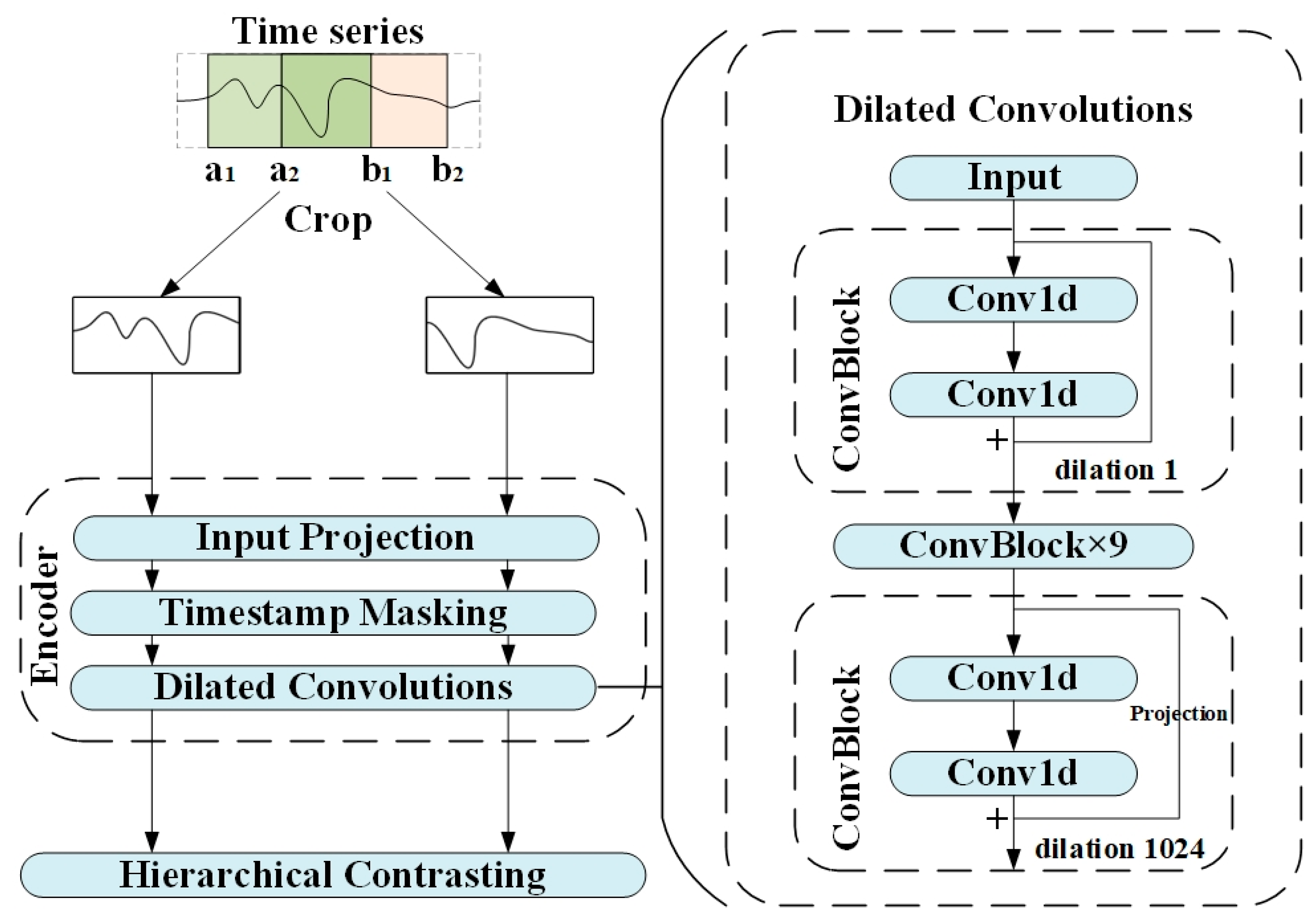
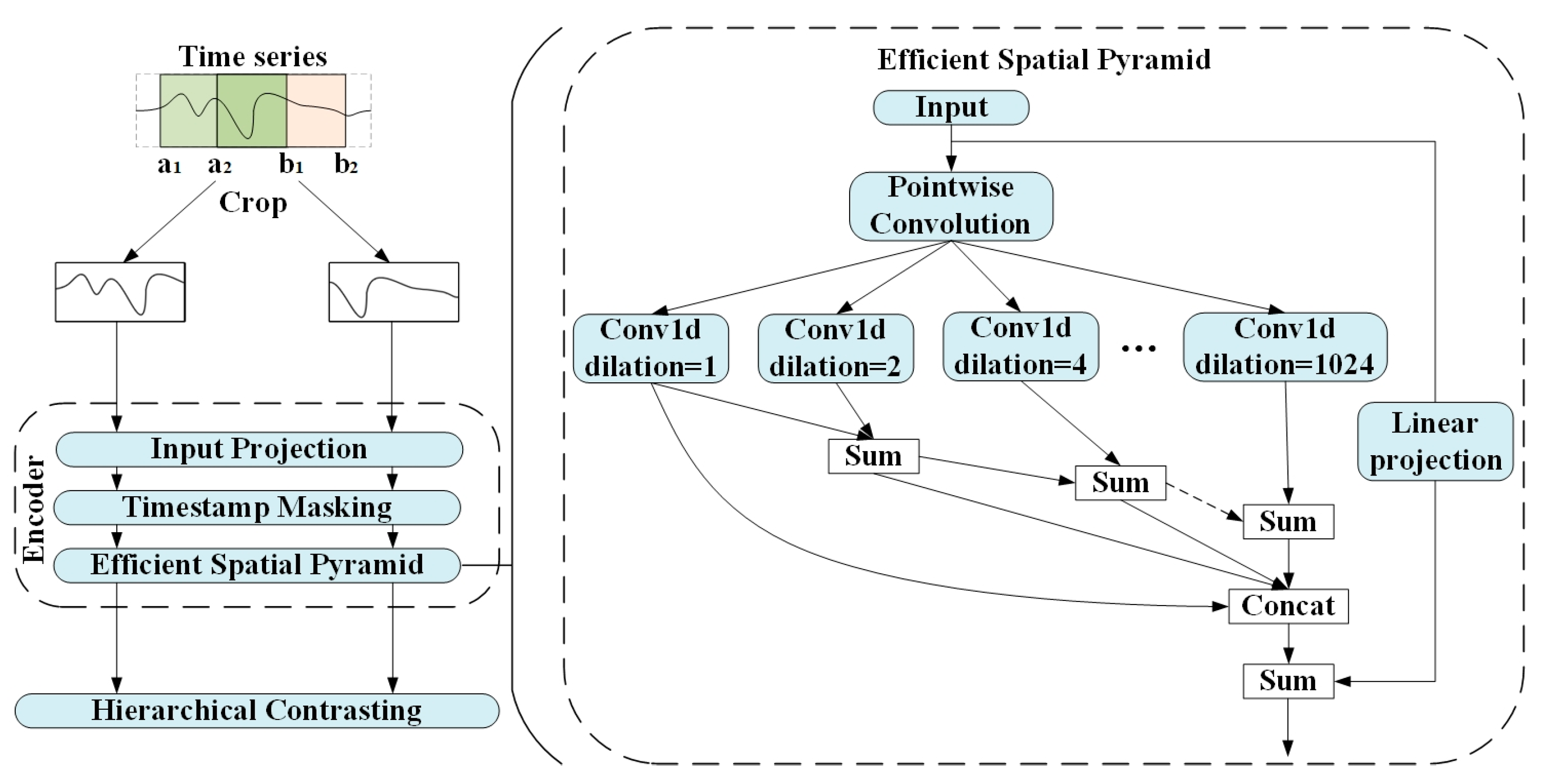
- In the lightweight representation learning stage, the dilated convolution part of the existing TS2Vec representation model is innovatively modified, and the efficient spatial pyramid structure is adopted, which better compensates for the gridding effect caused by the dilated convolution. This not only enhances the ability of the model to capture multi-scale features, but also improves the flexibility and adaptability of the model in dealing with complex time series data.
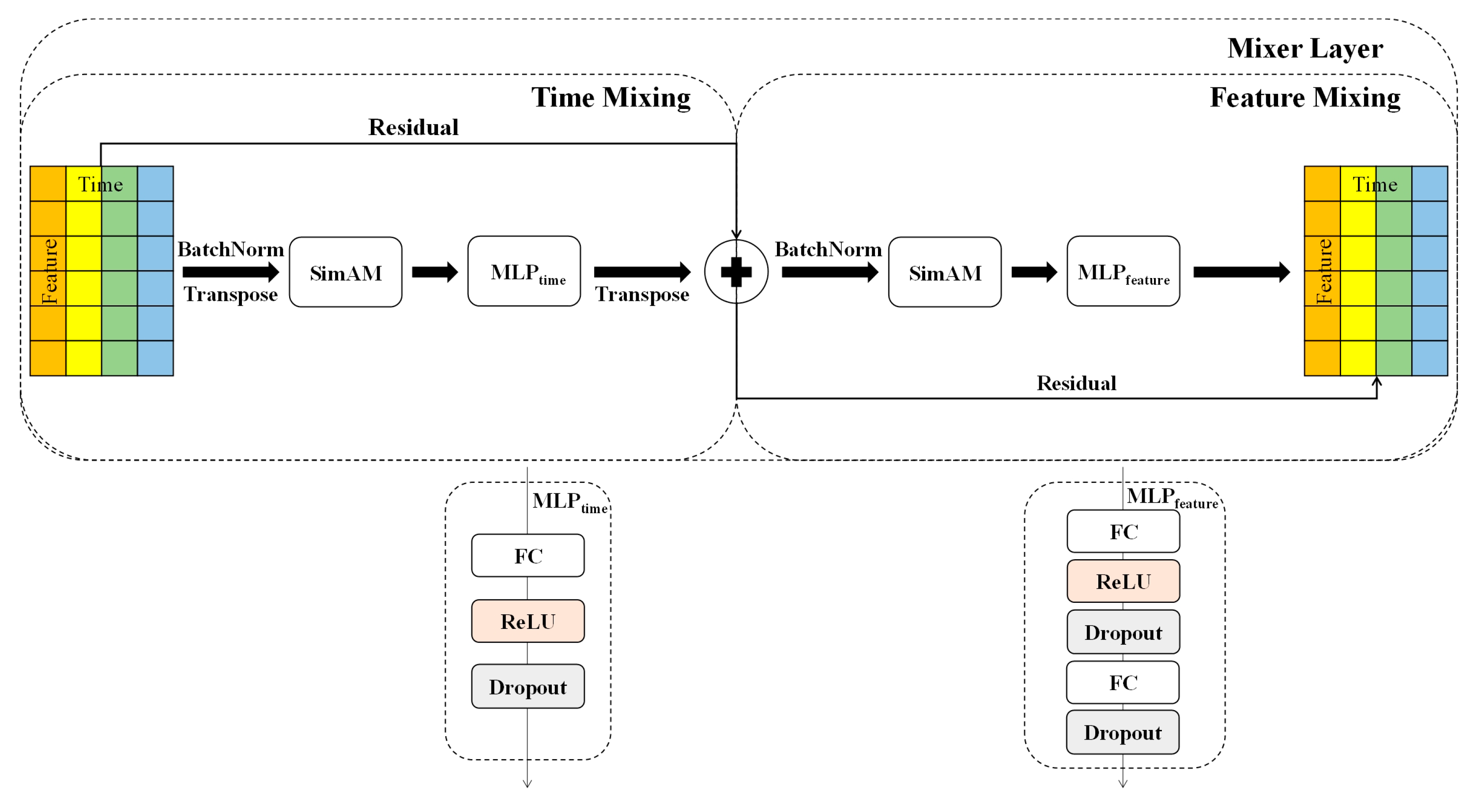
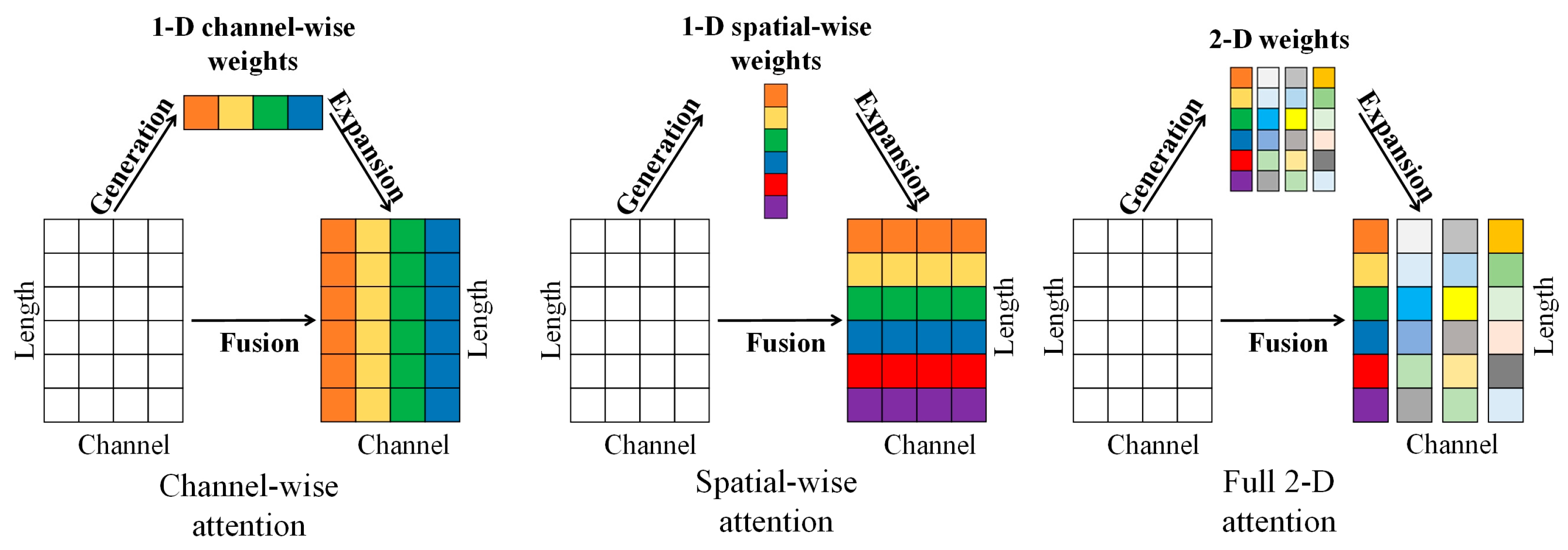
- In the multivariate feature mixing stage, a multivariate mixing layer is constructed based on the TSMixer architecture, which utilizes its cross-dimensional interaction mechanism to extract implicit associations among features, and embeds the SimAM lightweight attention mechanism, which adaptively adjusts the weights of the time steps through parameter-free computation to suppress the noise interference and enhance the contribution of key features.
2. Data
3. Methods and Results
3.1. Lightweight Representation Learning Model
3.1.1. Model Design
3.1.2. Model Testing and Result Analysis
3.2. Multivariate Feature Mixing Model
3.2.1. Model Design
3.2.2. Model Testing and Result Analysis
4. Discussion and Future Work
5. Conclusions
Author Contributions
Funding
Data Availability Statement
Conflicts of Interest
Abbreviations
| AI | Artificial Intelligence |
| SVM | Support Vector Machine |
| ANN | Artificial Neural Network |
| DNN | Deep Neural Network |
| CEEMDAN | Complete Ensemble Empirical Mode Decomposition with Adaptive Noise |
| EWT | Empirical Wavelet Transform |
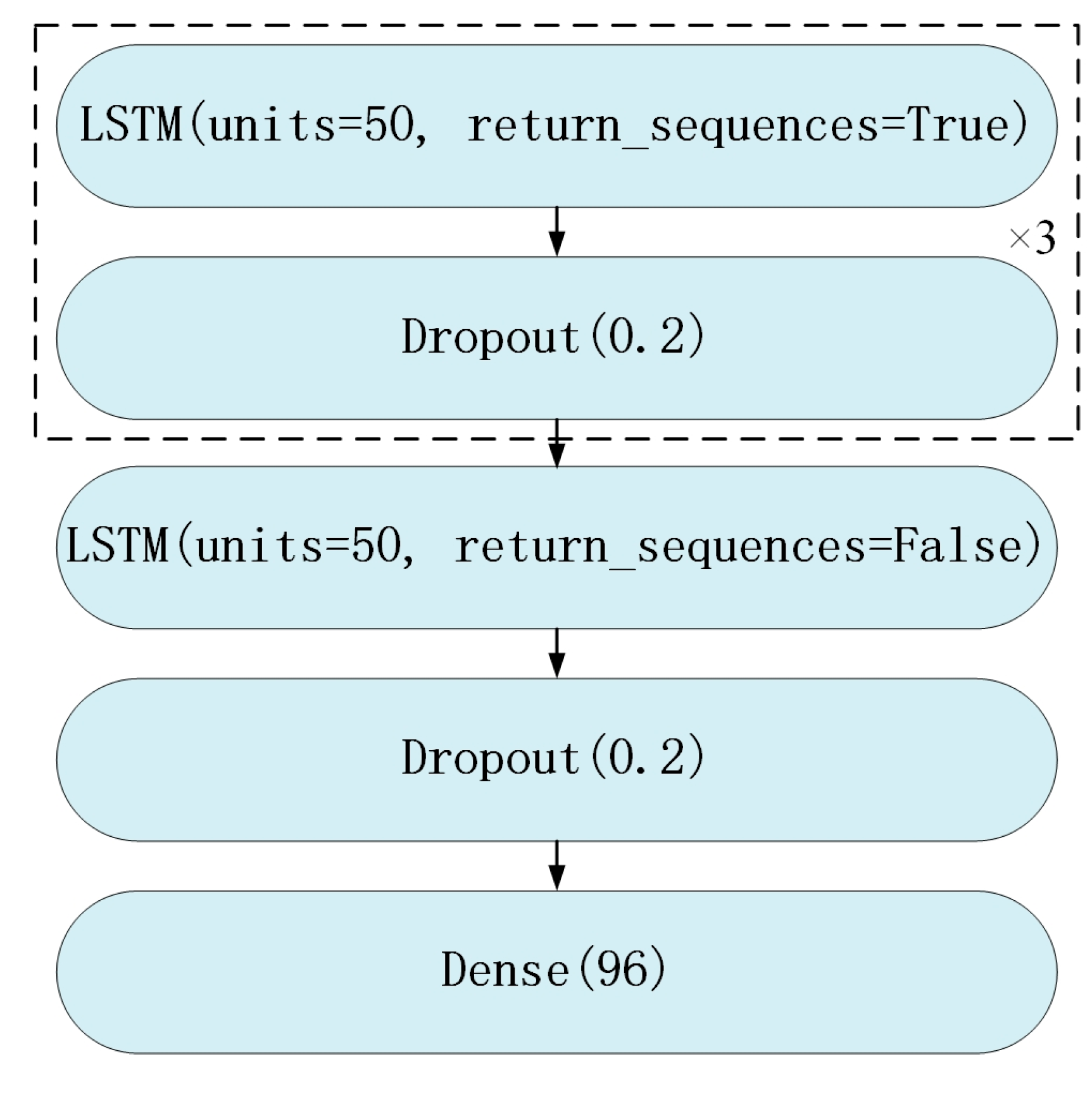
| LSTM | Long-Short Term Memory |
| ESPNet | Efficient Spatial Pyramid Net |
| PatchTST | Patch Time Series Transformer |
| SimAM | Similarity-Aware Activation Module |
| LLM4TS | Large Language Models for Time Series |
| LLM | Large Language Model |
| TSMixer | Time Series Mixer |
| MLP | Multilayer Perceptron |
| RNN | Recurrent Neural Network |
| FLOPs | Floating Point Operations |
| CPU | Central Processing Unit |
| GPU | Graphics Processing Unit |
| MAE | Mean Absolute Error |
| MSE | Mean Squared Error |
| RMSE | Root Mean Square Error |
References
- Nazir, M.S.; Wang, Y.; Bilal, M.; Abdalla, A.N. Wind energy, its application, challenges, and potential environmental impact. In Handbook of Climate Change Mitigation and Adaptation; Springer: Cham, Switzerland, 2022; pp. 899–935. [Google Scholar]
- Ahmed, S.D.; Al-Ismail, F.S.; Shafiullah, M.; Al-Sulaiman, F.A.; El-Amin, I.M. Grid integration challenges of wind energy: A review. IEEE Access 2020, 8, 10857–10878. [Google Scholar] [CrossRef]
- Tsai, W.-C.; Hong, C.-M.; Tu, C.-S.; Lin, W.-M.; Chen, C.-H. A review of modern wind power generation forecasting technologies. Sustainability 2023, 15, 10757. [Google Scholar] [CrossRef]
- Qiao, Y.; Lu, Z.; Min, Y. Research & application of raising wind power prediction accuracy. Power Syst. Technol. 2017, 41, 3261–3268. [Google Scholar]
- Zheng, Y.; Ge, Y.; Muhsen, S.; Wang, S.; Elkamchouchi, D.H.; Ali, E.; Ali, H.E. New ridge regression, artificial neural networks and support vector machine for wind speed prediction. Adv. Eng. Softw. 2023, 179, 103426. [Google Scholar] [CrossRef]
- Ateş, K.T. Estimation of short-term power of wind turbines using artificial neural network (ANN) and swarm intelligence. Sustainability 2023, 15, 13572. [Google Scholar] [CrossRef]
- Tarek, Z.; Shams, M.Y.; Elshewey, A.M.; El-kenawy, E.-S.M.; Ibrahim, A.; Abdelhamid, A.A.; El-dosuky, M.A. Wind Power Prediction Based on Machine Learning and Deep Learning Models. Comput. Mater. Contin. 2022, 74, 715–732. [Google Scholar] [CrossRef]
- Karijadi, I.; Chou, S.-Y.; Dewabharata, A. Wind power forecasting based on hybrid CEEMDAN-EWT deep learning method. Renew. Energy 2023, 218, 119357. [Google Scholar] [CrossRef]
- Chen, Y.; Zhao, H.; Zhou, R.; Xu, P.; Zhang, K.; Dai, Y.; Zhang, H.; Zhang, J.; Gao, T. CNN-BiLSTM short-term wind power forecasting method based on feature selection. IEEE J. Radio Freq. Identif. 2022, 6, 922–927. [Google Scholar] [CrossRef]
- Yousaf, S.; Bradshaw, C.R.; Kamalapurkar, R.; San, O. Investigating critical model input features for unitary air conditioning equipment. Energy Build. 2023, 284, 112823. [Google Scholar] [CrossRef]
- Yousaf, S.; Bradshaw, C.R.; Kamalapurkar, R.; San, O. A gray-box model for unitary air conditioners developed with symbolic regression. Int. J. Refrig. 2024, 168, 696–707. [Google Scholar] [CrossRef]
- Yue, Z.; Wang, Y.; Duan, J.; Yang, T.; Huang, C.; Tong, Y.; Xu, B. Ts2vec: Towards universal representation of time series. In Proceedings of the AAAI Conference on Artificial Intelligence, Online, 22 Februry–1 March 2022; pp. 8980–8987. [Google Scholar]
- Mehta, S.; Rastegari, M.; Caspi, A.; Shapiro, L.; Hajishirzi, H. Espnet: Efficient spatial pyramid of dilated convolutions for semantic segmentation. In Proceedings of the European Conference on Computer Vision (ECCV), Munich, Germany, 8–14 September 2018; pp. 552–568. [Google Scholar]
- Qiu, X.; Cheng, H.; Wu, X.; Hu, J.; Guo, C.; Yang, B. A comprehensive survey of deep learning for multivariate time series forecasting: A channel strategy perspective. arXiv 2025, arXiv:2502.10721. [Google Scholar]
- Sørensen, M.L.; Nystrup, P.; Bjerregård, M.B.; Møller, J.K.; Bacher, P.; Madsen, H. Recent developments in multivariate wind and solar power forecasting. Wiley Interdiscip. Rev. Energy Environ. 2023, 12, e465. [Google Scholar] [CrossRef]
- Nie, Y.; Nguyen, N.H.; Sinthong, P.; Kalagnanam, J. A time series is worth 64 words: Long-term forecasting with transformers. arXiv 2022, arXiv:2211.14730. [Google Scholar]
- Zeng, A.; Chen, M.; Zhang, L.; Xu, Q. Are transformers effective for time series forecasting? In Proceedings of the AAAI Conference on Artificial Intelligence, Washington, DC, USA, 7–14 February 2023; pp. 11121–11128. [Google Scholar] [CrossRef]
- Lin, S.; Lin, W.; Hu, X.; Wu, W.; Mo, R.; Zhong, H. Cyclenet: Enhancing time series forecasting through modeling periodic patterns. Adv. Neural Inf. Process. Syst. 2024, 37, 106315–106345. [Google Scholar]
- Han, L.; Ye, H.-J.; Zhan, D.-C. The capacity and robustness trade-off: Revisiting the channel independent strategy for multivariate time series forecasting. IEEE Trans. Knowl. Data Eng. 2024, 36, 7129–7142. [Google Scholar] [CrossRef]
- Chang, C.; Wang, W.-Y.; Peng, W.-C.; Chen, T.-F. Llm4ts: Aligning pre-trained llms as data-efficient time-series forecasters. ACM Trans. Intell. Syst. Technol. 2025, 16, 1–20. [Google Scholar] [CrossRef]
- Jin, M.; Wang, S.; Ma, L.; Chu, Z.; Zhang, J.Y.; Shi, X.; Chen, P.-Y.; Liang, Y.; Li, Y.-F.; Pan, S. Time-llm: Time series forecasting by reprogramming large language models. arXiv 2023, arXiv:2310.01728. [Google Scholar]
- Ansari, A.F.; Stella, L.; Turkmen, C.; Zhang, X.; Mercado, P.; Shen, H.; Shchur, O.; Rangapuram, S.S.; Arango, S.P.; Kapoor, S. Chronos: Learning the language of time series. arXiv 2024, arXiv:2403.07815. [Google Scholar]
- De Caro, F.; De Stefani, J.; Vaccaro, A.; Bontempi, G. DAFT-E: Feature-based multivariate and multi-step-ahead wind power forecasting. IEEE Trans. Sustain. Energy 2021, 13, 1199–1209. [Google Scholar] [CrossRef]
- Chen, S.-A.; Li, C.-L.; Yoder, N.; Arik, S.O.; Pfister, T. Tsmixer: An all-mlp architecture for time series forecasting. arXiv 2023, arXiv:2303.06053. [Google Scholar]
- Zheng, X.; Chen, X.; Schürch, M.; Mollaysa, A.; Allam, A.; Krauthammer, M. Simts: Rethinking contrastive representation learning for time series forecasting. arXiv 2023, arXiv:2303.18205. [Google Scholar]
- Yang, L.; Zhang, R.-Y.; Li, L.; Xie, X. Simam: A simple, parameter-free attention module for convolutional neural networks. In Proceedings of the International Conference on Machine Learning, Online, 18–24 July 2021; pp. 11863–11874. [Google Scholar]
- Shan, C.; Yuan, Z.; Qiu, Z.; He, Z.; An, P. A Dual Arrhythmia Classification Algorithm Based on Deep Learning and Attention Mechanism Incorporating Morphological-temporal Information. In Proceedings of the 2022 International Joint Conference on Neural Networks (IJCNN), Padua, Italy, 18–23 July 2022; pp. 1–8. [Google Scholar]
- Liu, F.T.; Ting, K.M.; Zhou, Z.-H. Isolation forest. In Proceedings of the 2008 Eighth IEEE International Conference on Data Mining, Pisa, Italy, 15–19 December 2008; pp. 413–422. [Google Scholar]
- Blu, T.; Thévenaz, P.; Unser, M. Linear interpolation revitalized. IEEE Trans. Image Process. 2004, 13, 710–719. [Google Scholar] [CrossRef] [PubMed]
- Ahsan, M.M.; Mahmud, M.P.; Saha, P.K.; Gupta, K.D.; Siddique, Z. Effect of data scaling methods on machine learning algorithms and model performance. Technologies 2021, 9, 52. [Google Scholar] [CrossRef]
- Greff, K.; Srivastava, R.K.; Koutník, J.; Steunebrink, B.R.; Schmidhuber, J. LSTM: A search space odyssey. IEEE Trans. Neural Netw. Learn. Syst. 2016, 28, 2222–2232. [Google Scholar] [CrossRef]
- Cerqueira, V.; Torgo, L.; Mozetič, I. Evaluating time series forecasting models: An empirical study on performance estimation methods. Mach. Learn. 2020, 109, 1997–2028. [Google Scholar] [CrossRef]
- Abnar, S.; Shah, H.; Busbridge, D.; Ali, A.M.E.; Susskind, J.; Thilak, V. Parameters vs flops: Scaling laws for optimal sparsity for mixture-of-experts language models. arXiv 2025, arXiv:2501.12370. [Google Scholar]
- Popescu, M.-C.; Balas, V.E.; Perescu-Popescu, L.; Mastorakis, N. Multilayer perceptron and neural networks. WSEAS Trans. Circuits Syst. 2009, 8, 579–588. [Google Scholar]
- Medsker, L.R.; Jain, L. Recurrent neural networks. Des. Appl. 2001, 5, 2. [Google Scholar]
- Oreshkin, B.N.; Carpov, D.; Chapados, N.; Bengio, Y. N-BEATS: Neural basis expansion analysis for interpretable time series forecasting. arXiv 2019, arXiv:1905.10437. [Google Scholar]
- Zhang, K.; Sun, M.; Han, T.X.; Yuan, X.; Guo, L.; Liu, T. Residual networks of residual networks: Multilevel residual networks. IEEE Trans. Circuits Syst. Video Technol. 2017, 28, 1303–1314. [Google Scholar] [CrossRef]
- Hollis, T.; Viscardi, A.; Yi, S.E. A comparison of LSTMs and attention mechanisms for forecasting financial time series. arXiv 2018, arXiv:1812.07699. [Google Scholar]
- Brauwers, G.; Frasincar, F. A general survey on attention mechanisms in deep learning. IEEE Trans. Knowl. Data Eng. 2021, 35, 3279–3298. [Google Scholar] [CrossRef]
- Lin, S.; Lin, W.; Wu, W.; Chen, H.; Yang, J. Sparsetsf: Modeling long-term time series forecasting with 1k parameters. arXiv 2024, arXiv:2405.00946. [Google Scholar]


| Model | MAE | MSE | RMSE |
|---|---|---|---|
| Original TS2Vec + LSTM | 0.6438 | 0.7305 | 0.8547 |
| Improved TS2Vec + LSTM | 0.6228 | 0.7268 | 0.8525 |
| Model | FLOPs | Params |
|---|---|---|
| Original TS2Vec + LSTM | 4.9659 G | 0.7110 M |
| Improved TS2Vec + LSTM | 0.4286 G | 0.0609 M |
| Model | MAE | MSE | RMSE |
|---|---|---|---|
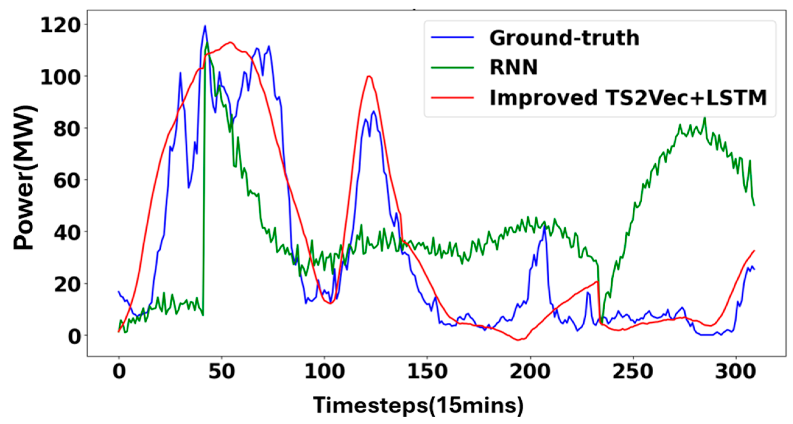
| MLP [34] | 0.7178 | 0.9589 | 0.9793 |
| RNN [35] | 0.7538 | 0.8680 | 0.9317 |
| N-BEATS [36] | 0.7001 | 0.8787 | 0.9374 |
| LSTM | 0.7380 | 0.9790 | 0.9895 |
| Original TS2Vec + LSTM | 0.6438 | 0.7305 | 0.8547 |
| Improved TS2Vec + LSTM | 0.6228 | 0.7268 | 0.8525 |
| Model | MAE | MSE | RMSE |
|---|---|---|---|
| Improved TS2Vec + LSTM | 0.6228 | 0.7268 | 0.8525 |
| Improved TS2Vec + SimAM + SparseTSF [40] | 0.6674 | 0.7202 | 0.8486 |
| TSMixer | 0.7053 | 0.8167 | 0.9037 |
| SimAM + TSmixer | 0.6673 | 0.7423 | 0.8615 |
| Original TS2Vec + TSMixer | 0.5404 | 0.4889 | 0.6992 |
| Original TS2Vec + SimAM + TSMixer | 0.5334 | 0.4721 | 0.6871 |
| Improved TS2Vec + TSMixer | 0.3780 | 0.2477 | 0.4977 |
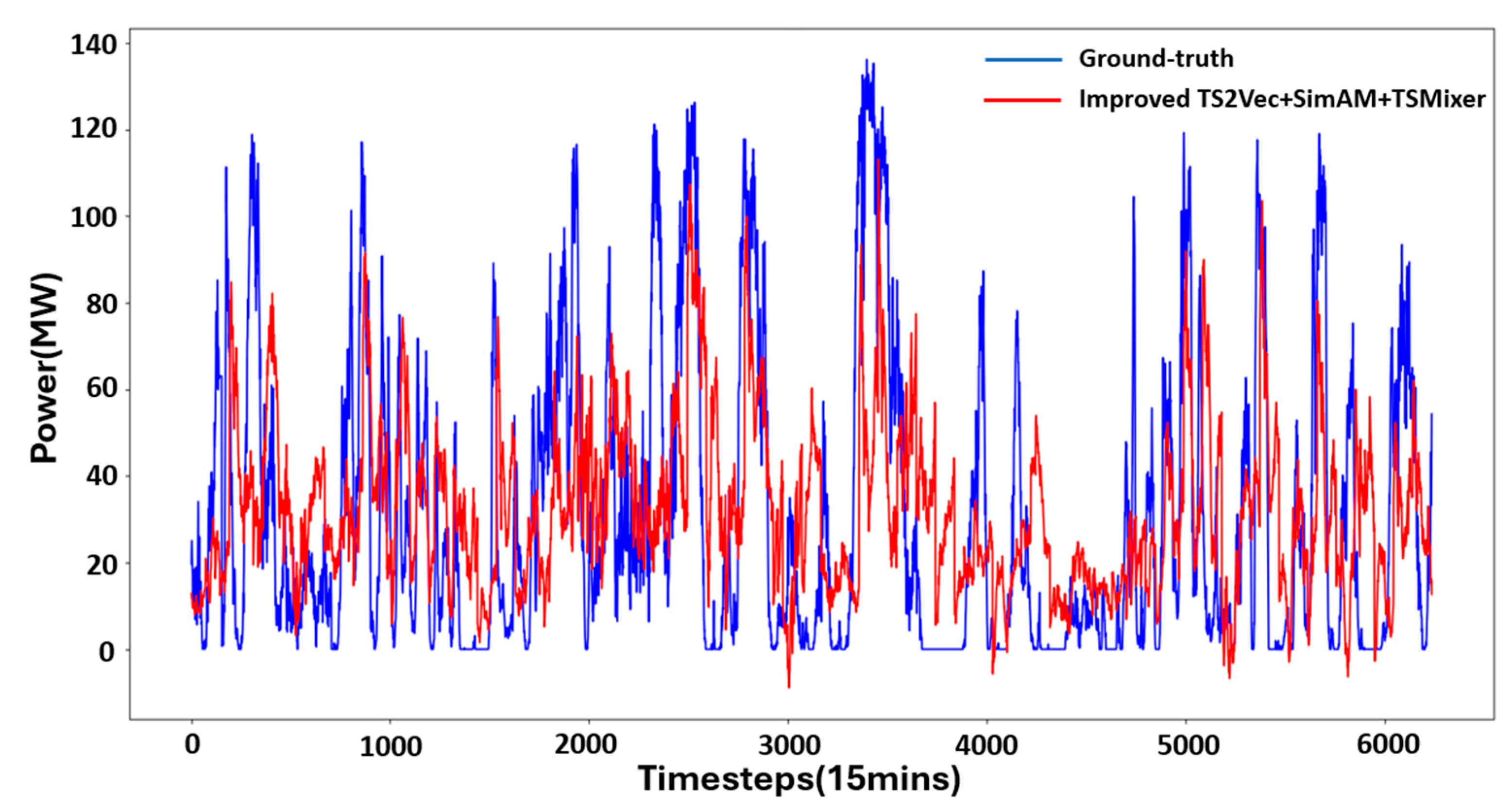
| Improved TS2Vec + SimAM + TSmixer | 0.3735 | 0.2434 | 0.4934 |
Disclaimer/Publisher’s Note: The statements, opinions and data contained in all publications are solely those of the individual author(s) and contributor(s) and not of MDPI and/or the editor(s). MDPI and/or the editor(s) disclaim responsibility for any injury to people or property resulting from any ideas, methods, instructions or products referred to in the content. |
© 2025 by the authors. Licensee MDPI, Basel, Switzerland. This article is an open access article distributed under the terms and conditions of the Creative Commons Attribution (CC BY) license (https://creativecommons.org/licenses/by/4.0/).
Share and Cite
Shan, C.; Liu, S.; Peng, S.; Huang, Z.; Zuo, Y.; Zhang, W.; Xiao, J. A Wind Power Forecasting Method Based on Lightweight Representation Learning and Multivariate Feature Mixing. Energies 2025, 18, 2902. https://doi.org/10.3390/en18112902
Shan C, Liu S, Peng S, Huang Z, Zuo Y, Zhang W, Xiao J. A Wind Power Forecasting Method Based on Lightweight Representation Learning and Multivariate Feature Mixing. Energies. 2025; 18(11):2902. https://doi.org/10.3390/en18112902
Chicago/Turabian StyleShan, Chudong, Shuai Liu, Shuangjian Peng, Zhihong Huang, Yuanjun Zuo, Wenjing Zhang, and Jian Xiao. 2025. "A Wind Power Forecasting Method Based on Lightweight Representation Learning and Multivariate Feature Mixing" Energies 18, no. 11: 2902. https://doi.org/10.3390/en18112902
APA StyleShan, C., Liu, S., Peng, S., Huang, Z., Zuo, Y., Zhang, W., & Xiao, J. (2025). A Wind Power Forecasting Method Based on Lightweight Representation Learning and Multivariate Feature Mixing. Energies, 18(11), 2902. https://doi.org/10.3390/en18112902