Optimizing Smart Grid Load Forecasting via a Hybrid Long Short-Term Memory-XGBoost Framework: Enhancing Accuracy, Robustness, and Energy Management

Abstract

As renewable energy sources and distributed generation become more integrated into modern power systems, accurate short-term electricity load forecasting is increasingly critical for effective smart grid management. Most statistical techniques used in the analysis of time series models, conventional statistical models, often fail to account for temporal dependencies and inherent non-linear patterns found in real-world energy time series. Methods: To this end, merging the power of both the ML approaches, namely Long Short-Term Memory (LSTM) networks and XGBoost, into hybrid frameworks has become a powerful solution. This work aims to develop a new compound model of LSTM for time series pattern extraction from the temporal data and XGBoost for outstanding predictive performance. To assess the performance of the proposed model, we used the Elia Grid dataset from Belgium, which includes load data recorded every 15 min throughout 2022. Results: When compared to individual models, this hybrid approach outperformed them, achieving a Root Mean Square Error (RMSE) of 106.54 MW, a Mean Absolute Percentage Error (MAPE) of 1.18%, and a coefficient of determination (R²) of 0.994. Discussion: In addition, this study implements an ensemble learning strategy by combining LSTM and XGBoost to improve prediction accuracy and robustness. An experimental attempt to integrate attention mechanisms was also conducted, but it did not enhance the performance and was therefore excluded from the final model. The results extend the literature on the development of fusion-based machine learning models for time series forecasting, and the future work of energy consumption analysis, anomaly detection, and resource allocation in SM grids.

1. Introduction

1.1. Background

The advancement in the industrial sector has accelerated the creation of data, especially time series data, which play an important role in various aspects such as finance, health care, climate forecasting, energy, and so on. Time series forecasting is the key to efficiency in resource management, organizational productivity enhancement, and the facilitating of operational decisions. Demand forecasting is critical in the energy sector for demand–supply management, the integration of renewables and managing the risk of power failures [1,2]. The improvement of computational efficiency has led to the application of machine learning (ML) and deep learning (DL) models in time series forecasting. Compared to statistical models like the ARIMA and SARIMA models, which are linear and stationary, ML models are well suited to non-linear, non-stationary, and high dimension processing [3]. In analyzing the sequential data, LSTM networks that belong to the RNN category have shown good results in expressing temporal relationships. Two major issues persist: comprehensiveness and interpretability [4,5]. In this work, an improved approach that combines the advantages of both LSTM and XGBoost has been advanced to increase accuracy as well as workability in time series data forecasting, where energy load prediction is used as a specific use case.

1.2. Research Goals and Methodology

This paper’s objective is to devise a high-performing yet balanced hybrid approach that incorporates LSTM networks and XGBoost to enable accurate, easily understandable predictions and demonstrate generalizability. The specific objectives are as follows:

• To examine the validity of other time series models in dealing with energy data as a means of understanding their strengths and weaknesses;
• To develop a new enhanced hybrid LSTM-XGBoost framework, with the ability to use temporal dependencies and feature the importance for improved prediction performance;
• For the purpose of assessing the effectiveness of the proposed model with actual energy datasets and comparing it with other standalone as well as conventional models;
• To create an understanding of how the hybrid model can be extended to practical applications and other domains.

The methodology consists of three key phases:

• Data Collection and Preprocessing: Raw energy load data is gathered for each time period in the historical database and aggregated, standardized or normalized as needed. Some variables may also be missing; therefore, the program employs state-of-the-art technology to conduct interpolation and ensure data quality [6];
• Model Development: LSTM is used to learn temporal dependencies, and predictions are refined through XGBoost. An attention mechanism was experimentally tested but not included in the final model due to the performance limitations;
• Evaluation and Comparison: Based on RMSE and MAPE, and compared with ARIMA, standalone LSTM, and XGBoost models.

The study addresses challenges such as data noise, high dimensionality, scalability [7], and computational complexity [8].

The inherent characteristics of electricity load data present significant forecasting challenges. These include sudden spikes, pronounced non-stationarity across daily, weekly, and seasonal cycles, and randomness stemming from unpredictable human consumption patterns. Given those peculiarities, LSTM was selected for its proven ability to capture both short-term fluctuations and long-term dependencies in non-stationary sequential data. Meanwhile, XGBoost complements this by efficiently correcting residual errors and modeling complex non-linear relationships, thus improving robustness to sudden anomalies. Although techniques such as ARIMA, Prophet, Random Forest, or SVM can be applied, their performance typically degrades on highly non-linear, non-stationary electricity-load datasets. Hence, the hybrid of LSTM (for sequential dependencies) and XGBoost (for residual error correction) offers a more suitable solution [9].

1.3. Proposed Solution and Relevance to Smart Grids

The hybrid LSTM-XGBoost model addresses these challenges by combining the temporal modeling capabilities of LSTM with the feature importance analysis of XGBoost. Key innovations include the following:

• Dynamic Feature Selection using XGBoost [10];
• Ensemble Learning to reduce variance and improve reliability [11].

The accurate forecasting of electricity load remains a major challenge in smart grid management. The increasing integration of solar and wind energy introduces additional complexity due to variability and intermittency. Additionally, the growing volume and variety of data generated by smart grid systems require advanced analytical techniques for effective decision-making [12].

Machine learning methods, especially deep learning and LSTM models, are promising in analyzing this data and predicting consumption trends with high accuracy [13,14]. LSTM networks can capture both short- and long-term dependencies, making them ideal for load forecasting in smart grids. This research focuses on leveraging LSTM for enhanced energy management and reliable grid operation.

2. Literature Review

2.1. Forecasting Techniques

The forecasting of data with time series has become an important aspect in the field of analytics mainly in the areas such as energy usage, finance, and health. The reconstruction of past values in an effort to forecast future occurrences is the basis of any planning or decision making. However, thanks to the machine learning (ML) and deep learning (DL) that have evolved ARIMA, it has become just another method to complement the growing list of sophisticated methods that can capture even intricate patterns in time series. In this chapter, the extensive methodologies of time series forecasting are examined, with a special emphasis on machine learning and deep learning algorithms. In more detail, it defines supervised and unsupervised learning techniques; intrinsically, the Long Short-Term Memory based Networks, the Hybrid models, the technique known as Ensemble learning, and the Attention mechanism utilized in time series forecasting.

Time series can be defined as the arrangement of values taken by a variable at a different time with a particular interval [14]. Used extensively in all sectors, including economic and financial forecasting and energy usage, this methodology employs methods that capture temporal features, trends, and seasons. However, the problem of data noise, missing data, and non-linear relationships in real-world data still remain cumbersome [15]. In responding to these challenges, there are short-term and long-term forecasting methods such as classical statistical models including autoregressive integrated moving average (ARIMA) and long short-term memory (LSTM).

In supervised learning methods, the model is trained with the help of the input datasets and the output value of the dataset is also known in advance. For instance, in regression, decision trees, neural networks, exponential smoothing, autoregressive integrated moving average (ARIMA), and others, have been used in time series problems [16]. For instance, XGBoost is an ensemble method that has a relatively high accuracy in forecast application due to the use of multiple weak models [17].

In contrast, unsupervised learning methods do not make use of training data and are used for the detection of features or artifacts that may not be recognizable to the model. Some of the approaches that can be used are: clustering algorithms such as K-means for grouping similar data points, and anomaly detection for the detection of sparse events in the data [18,19]. These techniques are great when one wants to scan the data for a suspicious pattern as is usually the case with IoT time series data or network traffic.

2.2. Deep Learning and Hybrid Models

More recently, deep learning models have emerged as popular for time series forecasting because of their capabilities to capture the features of the raw data without needing extensive feature engineering. Among these models, the LSTM networks as well as the GRU have been used most frequently to solve the problem of sequence prediction [20].

LSTM is a kind of Recurrent Neural Network that has long-term memory for the dependencies in sequence data. LSTM has been reported to be more accurate than traditional econometric models such as ARIMA in a range of application areas especially where there are intricate and non-linear linkages in the big data profiles [21]. For instance, LSTM models have been applied in energy load demand and in financial time series.

Gated Recurrent Units (GRU) is a much simpler model than the LSTM but with an equally good performance by combining the inputs and forget gates into a single gate. GRUs are less complex compared to LSTM and can still perform well in the time series forecasting tasks. They are especially successful in cases when a given set of data has long dependencies between values; for instance, in traffic or the weather prediction systems [22].

When LSTMs are combined with classical approaches such as ARIMA, they work better than when they are used individually in time series forecasting. This hybridizes the benefits of deep learning in temporal model representation and the dispensation of ARIMA in modeling trend and seasonality [23].

In the recent past, attention mechanisms and transformers have been widely used in sequential data tasks. These models can attend to parts of the input sequence, which can enhance performance during long-term predictions. Implementing transformers along with LSTM networks provide a way forward in capturing short- and long-term dependencies in time series data [24].

2.3. Hybrid Forecasting Models

More often, ensemble methods are one of the most effective groups of learning algorithms that involve the use of many models in prediction. This makes XGBoost a useful ensemble learning technique for time series forecasting as a result of its performance in dealing with large datasets and missing values [17]. Coupling LSTM networks with XGBoost incorporates the temporal feature extraction processes of the LSTM onto XGBoost’s prediction potential. The above models have been found to offer good improvements in accuracy when the data is noisy or non-linear.

Meta-learning or learning to learn has therefore proved useful in time series forecasting. In other words, it helps the models learn across several tasks, which in turns allows them to avoid complete retraining. For instance, in energy forecasting, meta-learning can learn to respond to such conditions as a one-off energy spurt or cyclical fluctuations in energy demand without requiring much extra information. Recent studies have used meta-learning to optimize for flexibility in various settings, most notably in renewable energy systems. This approach aids in solving some issues like the following: small dataset problems and different distributions [25].

The measures of performance are important in the assessment of the performance of the different forecasting models. Standard techniques involve Root Mean Squared Error (RMSE), Mean Absolute Error (MAE), and Mean Absolute Percentage Error (MAPE) [26]. These are employed to evaluate the performance of the models and to make the appropriate decisions concerning the suitability of certain mathematical models for specific uses.

Long-term forecasting capabilities are important for energy planning over days, months, or years in advance. However, long-horizon forecasting has problems including the accumulation of forecast errors and the identification of the macro signal. There are cases where the integration of the LSTM and XGBoost models works efficiently for such tasks because the LSTM has temporal aspects at its strong suit in addition to the long-term aspects of the XGBoost.

The problem of imbalance is acute in energy forecasting; thus, it provokes the occurrence of biases. For instance, events that have high demand, such as surge events, are rarely given much emphasis but are very necessary to be predicted well. Some algorithms; the Synthetic Minority Over-Sampling Technique (SMOTE) and Generative Adversarial Networks (GANs) are used to supplement the minority data by creating artificial data. These methods increase the model’s robustness and guarantee accurate forecasts across various conditions [27].

In transfer learning, one uses pre-training models from other related tasks to learn new related models faster and more accurately. In energy forecasting, what we have learnt is that an initial pre-trained model for a weather or traffic dataset can be used to train an approximate model for energy demand, thus reducing the time and computational power needed for training. It is even more applicable to areas with scarce tagged data, which includes specific areas or circumstances [28].

Hyperparameters are optimization parameters and the tuning of these parameters is very important for hybrid forecasting models. It is common knowledge that conventional approaches are either slow or involve substantial computational overheads. This task is automatically accomplished using other forms of evolutionary algorithms such as the genetic algorithms and particle swarm optimization to provide the best configurations for improved model performances. The usage of these techniques was affirmed on other similar hybrid models such as LSTM-XGBoost, where the performances of these models were enhanced and the number of ensuing attempts decreased [29].

Time series forecasting has evolved significantly with the advent of machine learning and deep learning techniques. Models like LSTMs, XGBoost, and hybrid approaches have demonstrated superior performance in various applications, from energy demand forecasting to financial prediction. The continued development of these models, particularly hybrid and ensemble learning techniques, holds promise for improving forecasting accuracy in complex and dynamic real-world systems. While attention mechanisms have been widely used in other forecasting studies, our empirical evaluation showed a limited benefit in the current hybrid setting. Therefore, they were excluded from the final model.

2.4. Large Language Models in Time Series Forecasting

Recent research has begun to examine the application of Large Language Models (LLMs) to time series forecasting. Unlike traditional numerical models, LLMs can integrate unstructured text information—like news, market reports, or policy updates—into forecast systems. One study proposed an LLM system that integrates real-time event analysis with electricity price forecasting, providing greater contextual precision through the inclusion of external indicators [30]. Another study introduced Time-LLM, a novel framework that achieved competitive results on common forecasting benchmarks by repurposing language models to handle and forecast temporal data via natural language prompts [31]. These advancements indicate promising avenues for combining LLMs with current sequence models, such as LSTM and XGBoost, especially for smart grid applications.

3. Proposed Methodology

In the interest of resolving the issues which are highlighted in the above section, this study adopts a methodology designed to develop a hybrid forecasting model for energy consumption in the Elia grid. Concerning the aim of the study, the main goal is to forecast energy load demand in the future, employing LSTM networks (implemented using TensorFlow, Google LLC., Mountain View, CA, USA) and functional XGBoost (DMLC, Seattle, WA, USA) in ways that demonstrate temporal and non-linear correlations in the data.

This hybrid approach gains the capability to explore the long-term temporal dependencies from LSTM and handle the non-linear data relationship from XGBoost. These equations and formulations are also worked out mathematically and included in this chapter for the construction of the models.

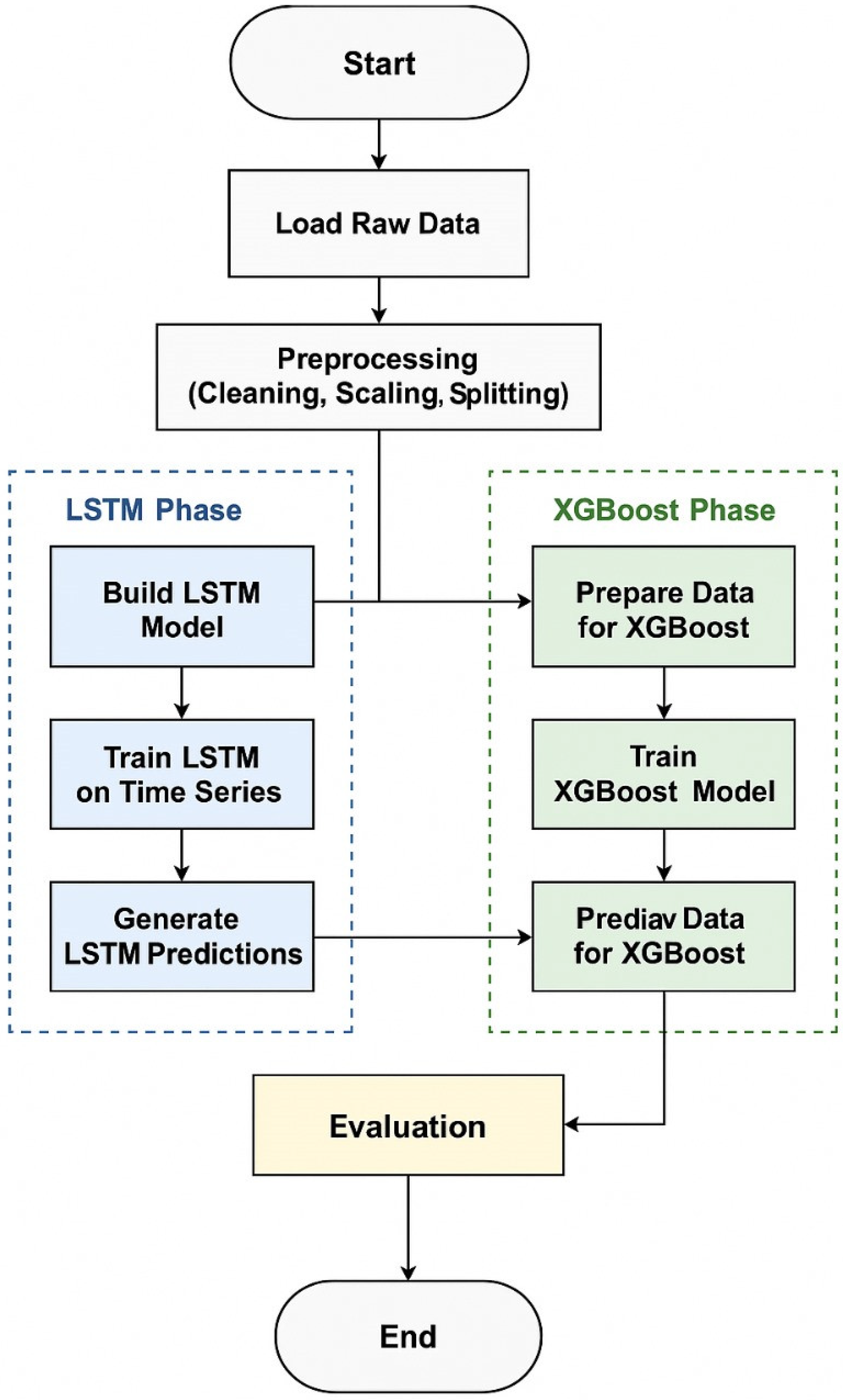
The work described is a two-fold approach of incorporating the LSTM and XGBoost models into the electric power distribution domain for improved accuracy. Every square on the diagram corresponds to a distinct phase of data processing, model training, and testing. The integration process takes advantage of a combination of two models; LSTM for sequence learning and XGBoost for a fine-tuning residual prediction model. Figure 1 provides a visual representation of the proposed hybrid forecasting methodology.

3.1. Data Preparation and Feature Engineering

The process begins with data loading, during which historical and real-time power distribution data are acquired. The common features of these datasets are the loading consumption, voltage levels, weather conditions, and operational parameters from the smart grid systems. This step makes it possible to make raw data available for the preprocessing part of the algorithm.

Preprocessing is crucial for improving the model performance:

• Scaling: There are still some procedures to be carried out prior to the normalization techniques (e.g., Min-Max scaling using scikit-learn, INRIA, Paris, France) to deal with the input features. This helps the values to remain within a certain vicinity and allow us to achieve convergence at the time of training [32].

$$X_{norm}={\displaystyle \frac{X-\min \left(X\right)}{\max \left(X\right)-\min \left(X\right)}}$$

(1)

where:

• $\mathit{X}$ is the original value;
• ${\mathit{X}}_{\mathit{n}\mathit{o}\mathit{r}\mathit{m}}$ is the normalized value;
• Splitting: The database is made up of training, validation, and implementation subsets because in this step, overfitting is avoided and it is possible to determine how good the model generalization is [33].

3.2. Model Development

3.2.1. LSTM Model

• The LSTM block involves the following:

• Model Definition: Creating LSTM to develop a pattern recognition of temporal flow of input data for the time-series data;
• Training: The model is built to maximize the probability of minimizing the Root Mean Square Error (RMSE) while extracting sequential data relationships. The initial predictions tend to contain some measure of error due to the temporal learning constraints.

3.2.2. Train and Predict with LSTM

This step involves making a prediction for the target variable; for example, load forecasting or fault detection, using the trained LSTM model. The outputs which are called LSTM Predictions are used to produce the final results and are intermediate values.

3.2.3. Prepare Data for XGBoost

As a result, residual errors in the LSTM predictions are removed before feeding the output to the XGBoost model through additional preprocessing. The first step stresses the identification of non-linear patterns and the second step enhances the prediction model’s quality.

$$e_t=y_t-{\widehat{y}}_t^{LSTM}$$

(2)

• ${\mathit{y}}_{\mathit{t}}$ is the actual observed value at time $\mathit{t}$;
• ${\widehat{\mathit{y}}}_{\mathit{t}}^{\mathit{L}\mathit{S}\mathit{T}\mathit{M}}$ is the predicted value at time $\mathit{t}$ generated by the LSTM model;
• ${\mathit{e}}_{\mathit{t}}$ is the residual error (difference) used as input to the XGBoost model.

3.2.4. Train XGBoost Model

The idea of the XGBoost component is that it learns from the residuals (the differences between the real values and the values predicted by the LSTM). While XGBoost is capable of handling high order interactions and non-linearity superimposing, the sequential learning power of the LSTM outperforms the results.

3.2.5. Make Predictions with XGBoost

In addition, unlike other classifiers, XGBoost gives better prediction results after training through the minimization of residual errors. This hybrid prediction is then combined with the output from the LSTM to complete the last step of the predictions from this step.

3.3. Model Evaluation

Finally, the hybrid model is evaluated against metrics such as the following:

• RMSE: Measures the accuracy of the prediction.

$$RMSE=\sqrt[]{{\displaystyle \frac{1}{n}}\sum _{i=1}^n{\left(y_i-\widehat{y_i}\right)}^2}$$

(3)

where:

• ${\mathit{y}}_{\mathit{i}}$ is the actual value;
• $\widehat{{\mathit{y}}_{\mathit{i}}}$ is the predicted value;
• $\mathit{n}$ is the total number of observations.
• MAPE: Indicates the percentage error, crucial for business insights.

$$\mathrm{M}\mathrm{A}\mathrm{P}\mathrm{E}={\displaystyle \frac{1}{n}}\sum _{t=1}^n \left|{\displaystyle \frac{y_t-{\widehat{y}}_t}{y_t}}\right|\times 100$$

(4)

• R² (Coefficient of Determination): Evaluates the model’s ability to explain variance in the data.

$$R^2=1-{\displaystyle \frac{{\sum }_{i=1}^N{\left(y_i-\widehat{y_i}\right)}^2}{{\sum }_{i=1}^N{\left(y_i-\overline{y}\right)}^2}}$$

(5)

The results are benchmarked against standalone models (e.g., LSTM, XGBoost) to validate the effectiveness of the hybrid approach.

3.4. Principal Benefits from the Hybrid Framework

• Improved Prediction Accuracy: This concept integrates the LSTM temporal learning with a non-linear XGBoost refinement;
• Error Reduction: able to capture the remaining errors which a single model may fail to detect;
• Scalability: suitable to be employed in different electric power distribution tasks; for instance, forecasting, outlier, or fault determination;
• Conceptual Enhancement: It is found that by adopting both LSTM and XGBoost, the proposed hybrid model acquires high accuracy and stability. This solution proves exceptionally appropriate when applied to the dynamic nature of the demands of the electric distribution systems.

3.5. Dataset and Preprocessing Overview

The dataset used in this study contains the hourly energy load data from Elia, Belgium’s transmission system operator, from January 1, 2022, to December 14, 2022. The dataset contains three key columns:

• Datetime (CET+1/CEST+2): local time in Central European Time (CET) or Central European Summer Time (CEST);
• Datetime (UTC): the corresponding Universal Time Coordinated (UTC) timestamp;
• Elia Grid Load [MW]: the measured grid load in megawatts.

A representative sample of the dataset is shown in Appendix A,

Table A1. Sample entries from Elia Grid Load dataset.

Datetime (CET/CEST)	Datetime (UTC)	Elia Grid Load\[MW]
1/1/2022 00:00	12/31/2021 23:00	7229.321
1/1/2022 00:15	12/31/2021 23:15	7141.165
1/1/2022 00:30	12/31/2021 23:30	7066.856
1/1/2022 00:45	12/31/2021 23:45	6956.022
1/1/2022 01:00	1/1/2022 00:00	6906.256

, to illustrate the structure and typical values.

Data cleaning ensures there are no missing, duplicate, or erroneous values. Missing values can be handled through interpolation or forward filling. Outliers in the grid load data are handled using the Interquartile Range (IQR) method.

Feature engineering added:

• Datetime Features: hour of the day, day of the week, month, and weekday indicator;
• Lag Features: previous grid loads (e.g., grid load at t−1t–1t−1, t−2t–2t−2);
• Rolling Window Features: mean, median, and standard deviation over the last NNN time periods.

The lag features are defined as:

$$X_{{lag}_k}(t)=y(t-k)$$

(6)

where:

• ${\mathit{X}}_{{\mathrm{lag} }_{\mathit{k}}}\left(\mathit{t}\right)$ is the lag feature at time t for lag k;
• $\mathit{y}(\mathit{t}-\mathit{k})$: the observed grid load at time $\mathit{t}-\mathit{k}$.

The rolling statistics are calculated as:

$$\begin{array}{c}\mathrm{Rolling}\mathrm{M}\mathrm{e}\mathrm{a}\mathrm{n}(t)={\displaystyle \frac{1}{N}}{\displaystyle \sum _{i=t-N+1}^t} y(i)\\ \mathrm{Rolling} \mathrm{S}\mathrm{t}\mathrm{d}(t)=\sqrt{{\displaystyle \frac{1}{N}}{\displaystyle \sum _{i=t-N+1}^t} (y(i)- \mathrm{Rolling} \mathrm{M}\mathrm{e}\mathrm{a}\mathrm{n}(t){)}^2}\end{array}$$

(7)

where $N$ is the window size.

For machine learning models, particularly deep learning models like the LSTM, the normalization of the data is crucial. The MinMaxScaler is used to scale the data to a range between 0 and 1.

To evaluate the model’s performance on unseen data, the dataset is split into training and testing sets. The training set consists of data from 1 January 2022 to 30 November 2022, while the testing set includes data from 1 December 2022 to 14 December 2022.

3.6. Model Architecture

3.6.1. LSTM Model

The LSTM model captures long-term temporal dependencies. Its architecture includes:

• LSTM Layers: memory cells for sequence learning;
• Dropout Layer: reduces overfitting;
• Dense Layer: final output prediction;
• The LSTM output at time t, denoted as h_t, is computed as the following:

$$h_t=\mathrm{L}\mathrm{S}\mathrm{T}\mathrm{M}\left(x_t,h_{t-1}\right)$$

(8)

where:

• ${\mathit{h}}_{\mathit{t}}$ is the hidden state of the LSTM at time $\mathit{t}$;
• ${\mathit{x}}_{\mathit{t}}$ is the input at time $\mathit{t}$;
• ${\mathit{h}}_{\mathit{t}-1}$ is the previous hidden state.

3.6.2. XGBoost Model

XGBoost is an ensemble learning model based on gradient boosting. It creates a committee of decision trees, where each tree tries to rectify the errors of the previous one. The prediction for an instance $\mathit{x}$ at step $\mathit{t}$ is calculated as follows:

$${\hat{y}}_t=\sum _{k=1}^T {\alpha }_k{f}_k(x)$$

(9)

where:

• ${\stackrel{\mathit{ˆ}}{\mathit{y}}}_{\mathit{t}}$ is the prediction at time $\mathit{t}$;
• ${\mathit{f}}_{\mathit{k}}\left(\mathit{x}\right)$ is the $\mathit{k}$-th tree’s prediction;
• $\mathit{T}$ is the total number of trees.

3.6.3. Hybrid Model

The hybrid model integrates LSTM and XGBoost to achieve high prediction accuracy by capturing both temporal and non-linear relationships in the data. The model is structured as follows:

• LSTM: The LSTM model is first applied and trains the energy load data to learn the temporal dependency and temporal sequence patterns;
• XGBoost: The output of the LSTM model, combined with the engineered features (e.g., lagged values, datetime features), is then fed to an XGBoost model.

The final prediction is obtained by applying the XGBoost regression model to the LSTM-generated output:

$${\hat{y}}_{\mathrm{final}}=f_{XGB}\left({\hat{y}}_{\mathrm{LSTM}}\right)$$

(10)

where ${\stackrel{\mathit{ˆ}}{\mathit{y}}}_{\mathrm{LSTM}}$ is the prediction generated by the LSTM model, and ${\mathit{f}}_{\mathit{XGB}}$ is the regression function learned by the XGBoost model. The final output ${\stackrel{\mathit{ˆ}}{\mathit{y}}}_{\mathit{final} }$ represents the improved forecast produced by applying the trained XGBoost model to the intermediate LSTM output.

4. Results and Analysis

The results of the forecasting models applied to the Elia Grid Load dataset are presented in this section. Model performance is assessed using RMSE, MAPE, and R². A comparison is also provided between individual models and the proposed hybrid approach.

4.1. Performance Metrics and Dataset Overview

The Elia Grid Load dataset contains the electricity load measurements from 1 January 2022 to 14 December 2022, with a 15 min resolution. It contains the UTC timestamps and corresponding load values in megawatts. Prior to modeling, the missing values were linearly interpolated, the load values were normalized to [0, 1], and the dataset was split into 80% training and 20% testing data.

To evaluate the model performance, the following metrics were used:

• Root Mean Square Error (RMSE);
• Mean Absolute Percentage Error (MAPE);
• Coefficient of Determination (R²).

4.2. Model Performance and Comparative Evaluation

• LSTM Model

The LSTM model was trained on the preprocessed data with a sequence length of 60 (15 min intervals for 15 h). The model’s architecture included two LSTM layers with 50 neurons each, followed by dense layers.

• XGBoostModel

The XGBoost model was trained with the same feature set as the LSTM. Key hyper parameters such as the number of estimators and learning rate were optimized using a grid search.

• Hybrid LSTM-XGBoost Model

A hybrid model combining the LSTM and XGBoost was implemented. The LSTM predicted short-term patterns, while XGBoost handled the long-term trends and residuals.

As shown in

Table 1. Comparative Results.

Model	RMSE (MW)	MAPE (%)	R2
LSTM	119.41	1.30	0.992
XGBoost	109.48	1.21	0.994
LSTM-XGBoost	106.54	1.18	0.994

, the hybrid model outperforms the individual models across all the evaluation metrics.

4.3. Visualization of Results

Visualizations of the model’s predictions against the actual consumption data provide a clear illustration of its performance. These visualizations include the time series plots, scatter plots, and heatmaps, offering different perspectives on the model’s accuracy and behavior.

4.3.1. Time Series of Actual Load

Figure 2 shows the comparison between the actual and predicted load values over a representative time period, demonstrating the close alignment between the model’s forecasts and the actual consumption patterns.

4.3.2. Scatter Plot of Actual vs. Predicted Values

Figure 3 presents a scatter plot of the actual electrical load over time. The plot exhibits a clear seasonal trend, with higher loads observed during the early and late months of the year and lower values in the middle of the year. This visualization helps identify consumption patterns and potential outliers in the dataset.

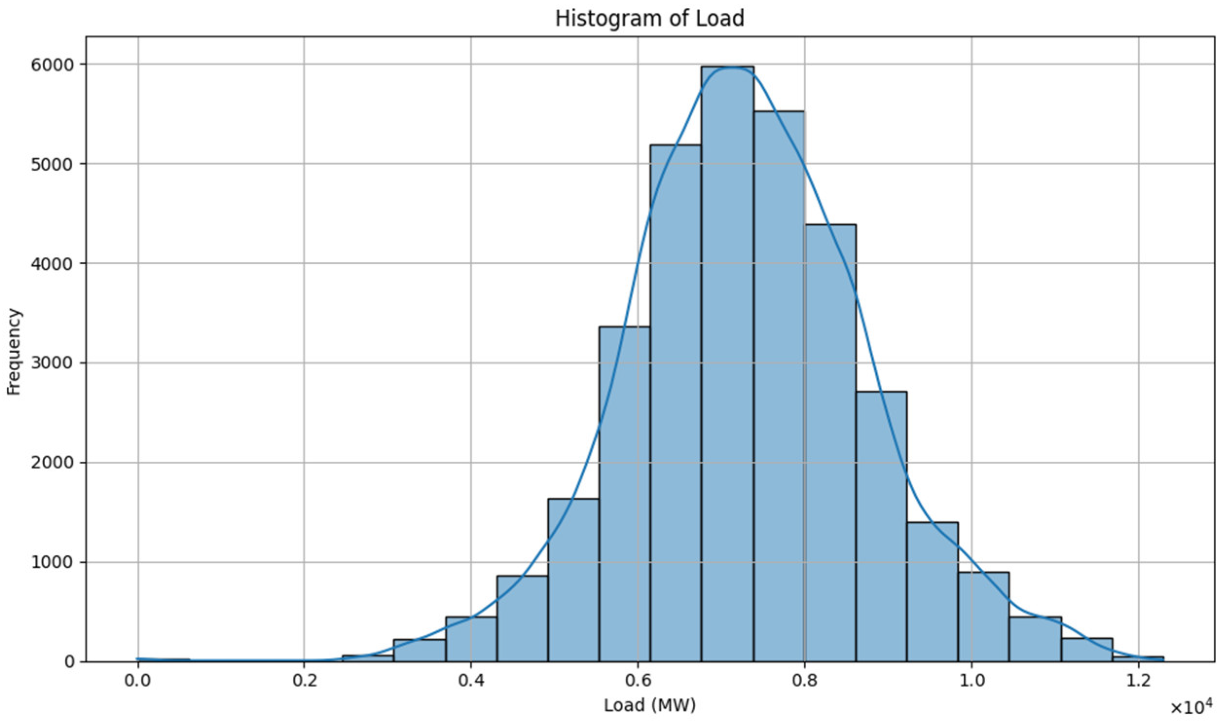
4.3.3. Histogram of Actual Load Values

Figure 4 presents a histogram of the actual electrical load values over the observation period. The distribution appears approximately normal, centered around the mean, with most load values falling within a moderate range. This pattern indicates consistent grid demand behavior, with fewer instances of extremely low or high consumption. The bell-shaped distribution also supports the assumption of stationarity and model generalization.

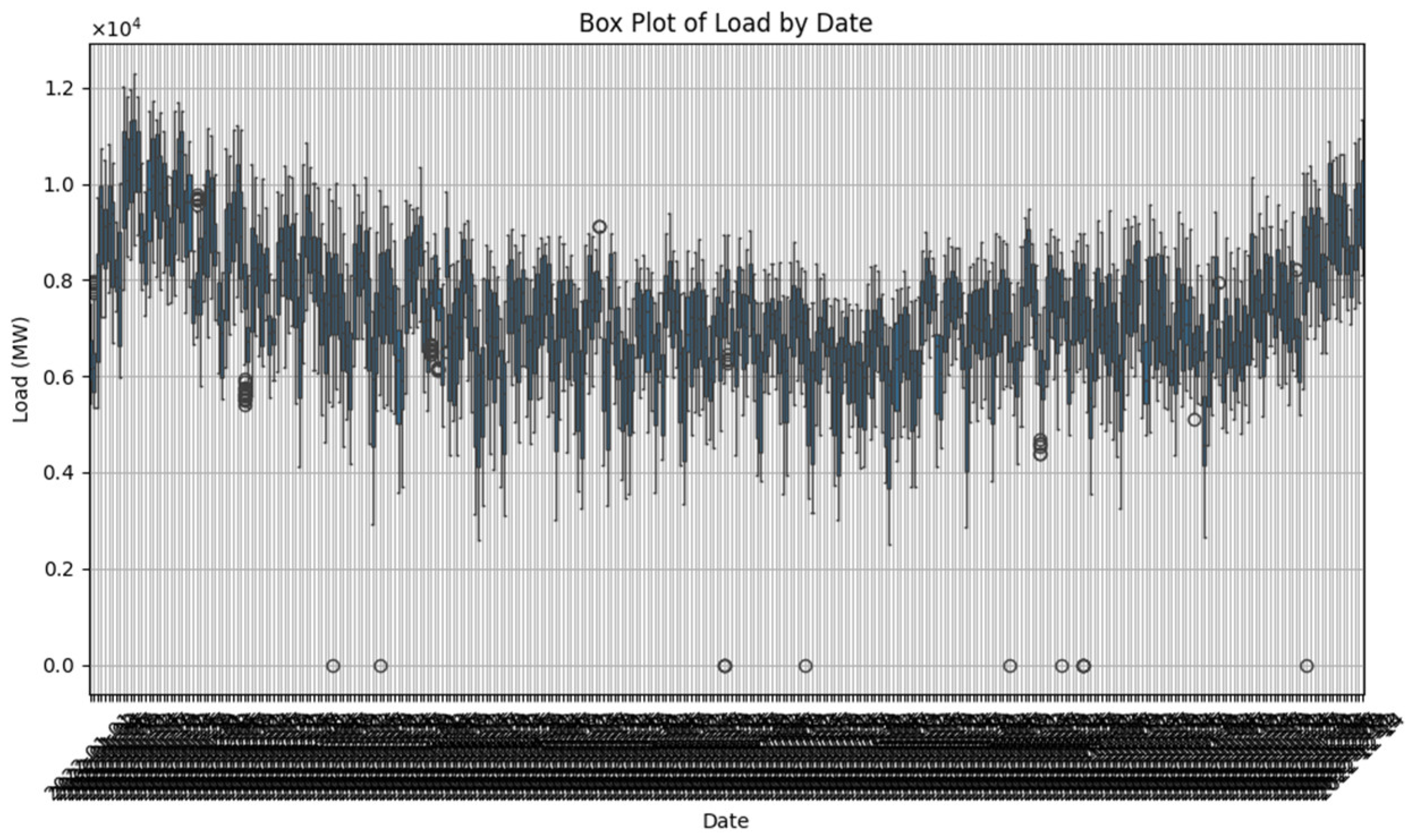
4.3.4. Box Plot Analysis

The box plot analysis (Figure 5) provides insights into the distribution of the load values across the different time periods. The analysis shows that most data points lie within the interquartile range, indicating a consistent model performance across various conditions.

The box plot also reveals the presence of outliers, which represent unusual consumption patterns that may require special attention in grid management. The model’s ability to identify and respond to these outliers is an important aspect of its utility for real-world applications.

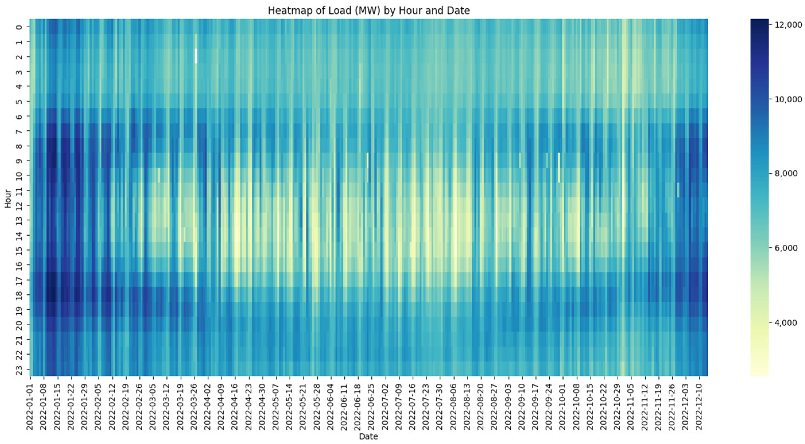
4.3.5. Heatmap of Load by Hour and Date

The heatmap of the load by hour and date (Figure 6) shows that the model captures the temporal characteristics of the load, including the day of the week. The model reflects the load changes throughout the hours and dates, hence enhancing the management and forecasting of the grid.

This visualization provides a comprehensive view of the consumption patterns across different dimensions, allowing for a deeper understanding of the factors influencing the electricity demand. Such insights are valuable for the grid operators in planning and optimizing the resource allocation.

4.3.6. Comparative Analysis

Compared to the conventional methods of forecasting and other machine learning algorithms, the LSTM has exhibited better accuracy, as well as its capability for generalization. The LSTM networks have been proven to have the capability to model the temporal patterns inherent in electricity consumption [34].

The superior performance of the LSTM networks can be attributed to their ability to maintain information over long sequences, which is particularly advantageous for capturing the long-term dependencies in time series data. This capability makes the LSTM networks well suited for load forecasting in smart grid applications, where both short-term and long-term patterns influence the electricity consumption.

4.4. Detailed Evaluation by Metric

The following discussion analyzes the results presented in Table 1 in detail, highlighting the strengths and weaknesses of each model across the three evaluation metrics.

4.4.1. Root Mean Square Error (RMSE):

• The combined LSTM-XGBoost model produces the lowest RMSE value, which is (106.54 MW), indicating its superior accuracy in minimizing prediction errors across all the evaluated models;
• The standalone XGBoost model achieved a moderate RMSE of (109.48 MW), showing a better performance than the LSTM but less accurate than the hybrid model;
• The LSTM model recorded the highest RMSE of (119.41 MW), reflecting its relative limitations in handling noise and complex patterns when used alone.

4.4.2. Mean Absolute Percentage Error (MAPE):

• The LSTM-XGBoost hybrid model records the lowest MAPE value of (1.18%), signifying its exceptional accuracy in forecasting energy demand with minimal relative errors;
• The XGBoost model records a MAPE (1.21%), showing slightly better accuracy than the LSTM model, but still not outperforming the hybrid model;
• The LSTM model achieves a MAPE of (1.30%), performing well in capturing the trends and patterns in the data.

4.4.3. Coefficient of Determination (R²):

• The LSTM-XGBoost hybrid model achieves one of the highest R² values (0.994), showcasing its superior ability to explain the variations in energy demand;
• The XGBoost model also achieves a high R² of (0.994), indicating a strong performance in capturing the overall variance despite lacking temporal modeling;
• The LSTM model follows closely with an R² of (0.992), effectively capturing temporal dependencies with a slightly lower overall explanatory power.

4.5. Visual Analysis and Benchmarking

The plot shown below compares the performance of the LSTM model with that of the ensemble model, specifically LSTM + XG Boost for the predicted target of the dataset. The chart presents actual data and the results of the models’ predictions, allowing a clear comparison. This comparison is visually presented in Figure 7, which illustrates the actual and predicted values generated by both models.

This multi-part figure presents a comparative analysis of the actual electricity load against the predictions from the various forecasting models.

• (a) Actual vs. Predicted Load (LSTM):

The performance of the LSTM model in forecasting the load over time is shown in this plot. Although some high-frequency variations are still less accurately modeled, the model generally matches the data quite well, particularly when it comes to identifying broad trends.

• (b) XGBoost-only Forecasting:

Demonstrates the output of the XGBoost model using a fixed look-back window. Despite its strong fit in many regions, the model’s efficacy in identifying the long-term patterns is limited by its inability to learn the temporal dependencies.

• (c) Comparison of LSTM and LSTM+XGBoost Predictions:

This comparison demonstrates how the ensemble model outperforms the standalone LSTM, with the hybrid model tracking the actual load more precisely, particularly during the dynamic load variations.

• (d) LSTM and Ensemble Model Predictions:

This subfigure provides a combined view of the training and test predictions from both the LSTM and the ensemble model.

• Actual Data (Blue Line):

Represent the actual values from the dataset, serving as the benchmark for evaluating the predictive accuracy;

2.

LSTM Predictions (Orange Line):

Show the accuracy of the LSTM model on the training dataset. The LSTM network seems to learn the overall trends and patterns well but is less able to easily manage the high amplitude fluctuations or noise;

3.

LSTM Test Predictions (Green Line):

Show the predicted values on the test set according to the LSTM model. These enable the evaluator to reach a conclusion on the capability of the model in estimating on unknown data;

4.

Ensemble Test Predictions (Red Line):

Illustrate the predictions of the ensemble model using the LSTM outputs with an XGBoost regressor. This method improves the prediction stability and accuracy, especially during the changes.

• Insights Derived from the Graph:

• Model Performance Comparison:
  The ensemble model (Red line) demonstrates a superior accuracy compared to the standalone LSTM model, particularly in the test phase. This is evident from the closer alignment between the ensemble predictions and the actual data.

• Error Reduction:
  The ensemble approach helps mitigate errors observed in the LSTM model, especially in periods of high volatility. This suggests that combining different models can improve the overall predictive robustness.

• Practical Implications:
  This visualization underscores the effectiveness of ensemble methods in time-series forecasting tasks, highlighting their potential to address challenges such as overfitting and underfitting, which are common in LSTM models alone.

• Error Analysis:

• The LSTM model struggles during sudden spikes in demand, as it relies on sequential dependencies and fails to capture extreme anomalies.
• The XGBoost model exhibits a lower sensitivity to spikes but underperforms for continuous patterns due to its limited temporal modeling capabilities.
• The hybrid model combines the strengths of both, demonstrating improved accuracy and robustness.

4.6. Comparative Evaluation with Existing Models

To assess the performance of the proposed hybrid LSTM-XGBoost model, a comparative analysis is conducted against recent state-of-the-art forecasting models from the literature.

Table 2. Comparison of forecasting models. Note: N.R. = Not Reported; GWh = Gigawatt-hour; MAPE = Mean Absolute Percentage Error; RMSE = Root Mean Square Error; R² = Coefficient of Determination.

Study	Model/Method	Data Source	Metrics	Key Findings
This Study	LSTM-XGBoost (Hybrid)	Elia Grid (Belgium)—15 min	RMSE: 106.54 MW MAPE: 1.18% R2: 0.994	Highest accuracy; LSTM outputs fed directly into XGBoost allowing automatic residual correction, resulting in a more effective and integrated model.
[35]	ARIMA-LSTM (Hybrid)	Southern China Grid—Hourly data	RMSE: N.R. MAPE: 2.828 R2: 0.9732	Dynamic weighting between ARIMA and LSTM based on training error. Used lower-resolution data.
[36]	TimeGAN-CNN-LSTM	Industrial/Commercial (China), 15 min	RMSE: N.R. MAPE: 4.486% R2: 0.812	TimeGAN for synthetic data; CNN + LSTM hybrid for fast short-term load forecasting
[37]	Deep Learning Regression	Panama Grid, hourly	RMSE: 50.34 MW MAPE: 2.90% R2: 0.93	Dense NN (3 layers × 95 units); best 1-h forecast result among tested ML/DL models
[38]	CNN-BiLSTM-Attention	Guangzhou Grid (China), 15 min, seasonal	RMSE: 0.77 GWh MAPE: 1.08–1.67% R2: 0.985–0.991	Seasonal models; CEEMDAN + K-Means + VMD decomposition; strong results across four seasons
[39]	CNN-LSTM (Hybrid)	NTDC (Pakistan), hourly	RMSE: 538.71 MAPE: 2.72% R2: N.R.	Review + Simulation; model tested on NTDC data

summarizes selected studies from 2022 to 2025, including their employed methodologies, datasets, forecasting intervals, and performance metrics such as RMSE, MAPE, and R².

To put the performance of our proposed LSTM-XGBoost hybrid in context, a clear comparison with recent models is necessary. The model in [35] combines the LSTM and ARIMA by dynamically weighting their outputs. Although this hybrid adds statistical insight, it was tested on hourly resolution data, which simplifies the forecasting task due to reduced temporal volatility. In contrast, our model focuses on 15 min real-world grid data, which increases the complexity of the forecasting process while also enhancing its practical relevance.

In [36], TimeGAN, CNN, and LSTM are integrated to improve the forecasting performance in commercial and industrial buildings. While using TimeGAN to generate synthetic data increases training diversity, it may raise generalization concerns in real-world operational environments. Our model maintains pattern fidelity without artificial bias, since it is trained solely on real grid data.

The DNN-based model in [37] reported lower RMSE values, but on hourly national-level data, which naturally smooths out fluctuations and short-term variations. This makes their task less sensitive to rapid demand changes, unlike our model, which handles 15 min data with higher temporal granularity.

Study [38] achieves notable accuracy using a deep CNN-BiLSTM-Attention architecture, supported by CEEMDAN, VMD, and K-means for preprocessing and decomposition. Although this approach performs well across the seasons, the additional preprocessing complexity could limit its scalability in real-time applications.

Lastly, [39] presents a thorough simulation-based evaluation of CNN-LSTM hybrids. Although insightful, the reported RMSE (538.71 MW) is significantly higher, likely due to the differences in the modeling approach and the data characteristics.

Overall, while each study brings unique strengths in the design or preprocessing, our model offers a solid balance between the accuracy, simplicity, and temporal resolution, making it well suited for realistic short-term forecasting in modern smart grid environments.

This weakness in terms of the accuracy representing the time series of the electricity load is clearly demonstrated in the results shown in the analysis, whereby the integrated models particularly the LSTM-XGBoost significantly outperform the individual models. This result concurs with the literature from previous studies that examined the impact of the integration of neural networks with other ensemble learning models on forecast accuracy. However, despite its strong performance, the hybrid model presented some challenges during the development due to the architectural complexity of combining the two learning paradigms. Although the integration of the attention mechanisms was tested, the resulting accuracy was inferior to the base hybrid model. Therefore, attention was not included in the final implementation.

The details of the model performance evaluation of the electricity load forecasting were given in this chapter. This demonstrates that our optimal approach is the approach presented by the latter LSTM-XGBoost hybrid model, and identifies the importance of combining models as they have complementary weaknesses. The results obtained are suitable for further improvements related to the depicted architectural layouts.

5. Discussion and Conclusions

When comparing the performance of the three models: LSTM, XGBoost, and the LSTM-XGBoost model, significant disparities were established, and these disparities are crucial in terms of energy demand forecasting. The comparison was conducted using three major evaluation metrics: RMSE, MAPE, and the coefficient of determination (R²). The comparative analysis showed that for all four datasets the proposed LSTM-XGBoost hybrid model has better accuracy than the individual models. Thus, the Hybrid model combining the sequencing learning power of the LSTM with the boosting potential of XGBoost gave an overall lowest RMSE of 106.54 MW and the lowest MAPE of 1.18% with the highest R² value of 0.994.

On the other hand, there is moderate accuracy in the LSTM modeling the daily generation outputs with an RMSE of 119.41 MW and a slightly higher MAPE (1.30%) than the hybrid model. However, it was able to achieve a relatively reasonable R² value of 0.992, which would indicate the model’s capability of capturing the sequential patterns and other time-dependent characteristics of the energy demand.

The XGBoost model had a relatively better performance than the LSTM with an RMSE of 109.48 MW, MAPE of 1.21%, and an R² of 0.994. Despite being effective in general ML tasks, its application to the time-series data, where sequentiality is essential, still did not outperform the hybrid model.

Therefore, it can be seen that the hybrid LSTM-XGBoost model is superior and can minimize both absolute and relative errors. This finding corresponds with the previous research into the use of hybrid models capable of capturing both chronological and non-linear associations within large datasets.

The optimization of load forecasting can be a powerful tool in smart grids to improve energy management and reduce costs, including operational expenses, to provide a higher reliability of the grid. Accurate load forecasting enables better resource allocation, enhanced integration of renewable energy sources, and improved demand response strategies. The results of this present study will help in developing smart grid systems and integrating them into practical applications. The insights gained from this research contribute to the advancement of grid management techniques, supporting the transition toward more efficient and sustainable energy systems.

Future Work

Based on the findings of this study, several recommendations for future research can be made. To further improve the model performance, it is recommended that subsequent research incorporates datasets of greater sample size and diversity over time, incorporating a range of factors that may affect dependence such as seasonality, weather, or economic events. This would make the model more generalizable and reliable. Although accuracy has been improved by using the hybrid LSTM-XGBoost model, it is worth considering further hybridization of LSTM with other ensemble models like Random Forest or LightGBM. An integration of deep learning models such as GRU or Transformer models might also be a useful study.

Additionally, the application of advanced deep learning techniques may provide improvements in real-time forecasting scenarios. The findings should direct studies examining other feature engineering and selection methods to determine the most significant predictors of energy demand, aiding in decreasing complexity and increasing model efficacy. Although this paper was based on models and controls to evaluate the accuracy, deploying them in real-time software and dynamic energy systems adds challenges. It would be suitable for future work to consider practical use of these models in systems fed with real-world data streams that adapt parameter estimations as more data becomes available. Besides, other time series forecasting approaches including SARIMA and Prophet can also be explored to compare them with deep learning models.

Furthermore, future research will explore the model’s applicability to datasets from different regional grid operators, including hourly and daily resolutions, to assess its generalizability. In particular, we plan to evaluate the model using real-world electricity consumption data from the Iraqi national grid to enhance its practical relevance for local energy management systems.

Finally, future studies should include a systematic hyperparameter sensitivity analysis to evaluate the effect of the key configuration parameters—such as the number of LSTM units, the input sequence length, epochs, and train/test splits—on the model performance and robustness.

References

- Shering, T.; Alonso, E.; Apostolopoulou, D. Investigation of Load, Solar and Wind Generation as Target Variables in LSTM Time Series Forecasting, Using Exogenous Weather Variables. Energies 2024, 17, 1827. [Google Scholar] [CrossRef]
- Fan, G.F.; Peng, L.L.; Hong, W.C. Short-term load forecasting based on empirical wavelet transform and random forest. Electr. Eng. 2022, 104, 4433–4449. [Google Scholar] [CrossRef]
- Taieb, S.B.; Hyndman, R.J. A gradient boosting approach to the Kaggle load forecasting competition. Int. J. Forecast. 2014, 30, 382–394. [Google Scholar] [CrossRef]
- Interpretable Machine Learning. Available online: https://christophm.github.io/interpretable-ml-book/ (accessed on 20 May 2025).
- Casolaro, A.; Capone, V.; Iannuzzo, G.; Camastra, F. Deep Learning for Time Series Forecasting: Advances and Open Problems. Information 2023, 14, 598. [Google Scholar] [CrossRef]
- Ahn, H.; Sun, K.; Kim, K.P. Comparison of Missing Data Imputation Methods in Time Series Forecasting. Comput. Mater. Contin. 2021, 70, 767–779. [Google Scholar] [CrossRef]
- Vaswani, A.; Shazeer, N.; Parmar, N.; Uszkoreit, J.; Jones, L.; Gomez, A.N.; Kaiser, Ł.; Polosukhin, I. Attention Is All You Need. Adv. Neural Inf. Process. Syst. 2017, 2017, 5999–6009. Available online: https://arxiv.org/pdf/1706.03762 (accessed on 25 May 2025).
- Bandara, K.; Bergmeir, C.; Smyl, S. Forecasting across time series databases using recurrent neural networks on groups of similar series: A clustering approach. Expert Syst. Appl. 2020, 140, 112896. [Google Scholar] [CrossRef]
- Semmelmann, U.; Henni, S.; Weinhardt, C. Load forecasting for energy communities: A novel LSTM-XGBoost hybrid model based on smart meter data. Energy Inform. 2022, 5, 24. [Google Scholar] [CrossRef]
- Cui, J.; Kuang, W.; Geng, K.; Bi, A.; Bi, F.; Zheng, X.; Lin, C. Advanced Short-Term Load Forecasting with XGBoost-RF Feature Selection and CNN-GRU. Processes 2024, 12, 2466. [Google Scholar] [CrossRef]
- Kong, W.; Ding, Y.; Su, Z. Electrometallurgical Load Forecasting Based on Ensemble Learning Using CEEMDAN. J. Phys. Conf. Ser. 2022, 2356, 012028. [Google Scholar] [CrossRef]
- Zhang, J.; Zheng, Y.; Qi, D. Deep Spatio-Temporal Residual Networks for Citywide Crowd Flows Prediction. In Proceedings of the Thirty-First AAAI Conference on Artificial Intelligence, San Francisco, CA, USA, 4–9 February 2017; pp. 1655–1661. [Google Scholar] [CrossRef]
- Deep Learning for Time Series Forecasting. Available online: https://machinelearningmastery.com/deep-learning-for-time-series-forecasting/ (accessed on 21 April 2025).
- Shumway, R.H.; Stoffer, D.S. Time Series Analysis and Its Applications; Springer: New York, NY, USA, 2017. [Google Scholar] [CrossRef]
- Zhou, Y.; Aryal, S.; Bouadjenek, M.R. Review for Handling Missing Data with Special Missing Mechanism. 2024. Available online: https://arxiv.org/pdf/2404.04905 (accessed on 21 April 2025).
- Hyndman, R.J.; Athanasopoulos, G. Forecasting: Principles and Practice, 3rd ed.; OTexts: Melbourne, Australia, 2021; Available online: https://otexts.com/fpp3/ (accessed on 17 April 2025).
- Chen, T.; Guestrin, C. XGBoost: A scalable tree boosting system. In Proceedings of the ACM SIGKDD International Conference on Knowledge Discovery and Data Mining, New York, NY, USA, 13–17 August 2016; pp. 785–794. [Google Scholar]
- Abdullah, A.; Qureshi, M.A. Unsupervised learning techniques for IoT time series. Sens. Actuators A Phys. 2022, 336, 112–119. [Google Scholar]
- Chandola, V.; Banerjee, A.; Kumar, V. Anomaly detection. ACM Comput. Surv. 2009, 41, 1–58. [Google Scholar] [CrossRef]
- Fawaz, H.I.; Forestier, G.; Weber, J.; Idoumghar, L.; Muller, P.A. Deep learning for time series classification: A review. Data Min. Knowl. Discov. 2019, 33, 917–963. [Google Scholar] [CrossRef]
- Siami-Namini, S.; Tavakoli, N.; Namin, A.S. A Comparison of ARIMA and LSTM in Forecasting Time Series. In Proceedings of the 17th IEEE International Conference on Machine Learning and Applications, ICMLA, Orlando, FL, USA, 17–20 December 2018; pp. 1394–1401. [Google Scholar] [CrossRef]
- Nejadettehad, A.; Mahini, H.; Bahrak, B. Short-term Demand Forecasting for Online Car-hailing Services using Recurrent Neural Networks. Appl. Artif. Intell. 2019, 34, 674–689. [Google Scholar] [CrossRef]
- Huang, X.; Zhuang, X.; Tian, F.; Niu, Z.; Chen, Y.; Zhou, Q.; Yuan, C. A Hybrid ARIMA-LSTM-XGBoost Model with Linear Regression Stacking for Transformer Oil Temperature Prediction. Energies 2025, 18, 1432. [Google Scholar] [CrossRef]
- Lim, B.; Arık, S.Ö.; Loeff, N.; Pfister, T. Temporal Fusion Transformers for interpretable multi-horizon time series forecasting. Int. J. Forecast. 2021, 37, 1748–1764. [Google Scholar] [CrossRef]
- Meng, Z.; Guo, Y.; Sun, H. An Adaptive Approach for Probabilistic Wind Power Forecasting Based on Meta-Learning. IEEE Trans. Sustain. Energy 2023, 15, 1814–1833. [Google Scholar] [CrossRef]
- Botchkarev, A. A New Typology Design of Performance Metrics to Measure Errors in Machine Learning Regression Algorithms. Interdiscip. J. Inf. Knowl. Manag. 2019, 14, 045–076. [Google Scholar] [CrossRef]
- Chereddy, N.V.; Bolla, B.K. Evaluating the Utility of GAN Generated Synthetic Tabular Data for Class Balancing an d Low Resource Settings. In Lecture Notes in Computer Science (including subseries Lecture Notes in Artificial Intelligence and Lecture Notes in Bioinformatics); Springer Nature: Cham, Switzerland, 2023; Volume 14078 LNAI, pp. 48–59. [Google Scholar] [CrossRef]
- Sarmas, E.; Dimitropoulos, N.; Marinakis, V.; Mylona, Z.; Doukas, H. Transfer learning strategies for solar power forecasting under data scarcity. Sci. Rep. 2022, 12, 14643. [Google Scholar] [CrossRef]
- Mehdary, A.; Chehri, A.; Jakimi, A.; Saadane, R. Hyperparameter Optimization with Genetic Algorithms and XGBoost: A Step Forward in Smart Grid Fraud Detection. Sensors 2024, 24, 1230. [Google Scholar] [CrossRef]
- Gafni, Y.; Gradwohl, R.; Tennenholtz, M. Prediction-sharing During Training and Inference. 2024. Available online: https://arxiv.org/pdf/2403.17515 (accessed on 19 May 2025).
- Jin, M.; Wang, S.; Ma, L.; Chu, Z.; Zhang, J.Y.; Shi, X.; Chen, P.Y.; Liang, Y.; Li, Y.F.; Pan, S.; et al. Time-LLM: Time Series Forecasting by Reprogramming Large Language Models. In Proceedings of the 12th International Conference on Learning Representations, ICLR 2024, Vienna, Austria, 7–11 May 2024; Available online: https://arxiv.org/pdf/2310.01728 (accessed on 19 May 2025).
- Brownlee, J. How to Normalize and Standardize Time Series Data in Python. 2019. Available online: https://machinelearningmastery.com/normalize-standardize-time-series-data-python/ (accessed on 3 April 2025).
- López, O.A.M.; López, A.M.; Crossa, D.J. Overfitting, Model Tuning, and Evaluation of Prediction Performance. In Multivariate Statistical Machine Learning Methods for Genomic Prediction; Springer International Publishing: Cham, Switzerland, 2022; pp. 109–139. [Google Scholar] [CrossRef]
- Wang, K.; Zhang, J.; Li, X.; Zhang, Y. Long-Term Power Load Forecasting Using LSTM-Informer with Ensemble Learning. Electronics 2023, 12, 2175. [Google Scholar] [CrossRef]
- Zhou, R.; Zhang, X. Short-term power load forecasting based on ARIMA-LSTM. J. Phys. Conf. Ser. 2024, 2803, 012002. [Google Scholar] [CrossRef]
- Liu, Y.; Liang, Z.; Li, X. Enhancing Short-Term Power Load Forecasting for Industrial and Commercial Buildings: A Hybrid Approach Using TimeGAN, CNN, and LSTM. IEEE Open J. Ind. Electron. Soc. 2023, 4, 451–462. [Google Scholar] [CrossRef]
- Ibrahim, B.; Rabelo, L.; Gutierrez-Franco, E.; Clavijo-Buritica, N. Machine Learning for Short-Term Load Forecasting in Smart Grids. Energies 2022, 15, 8079. [Google Scholar] [CrossRef]
- Liu, X.; Song, J.; Tao, H.; Wang, P.; Mo, H.; Du, W. Quarter-Hourly Power Load Forecasting Based on a Hybrid CNN-BiLSTM-Attention Model with CEEMDAN, K-Means, and VMD. Energies 2025, 18, 2675. [Google Scholar] [CrossRef]
- Ullah, K.; Ahsan, M.; Hasanat, S.M.; Haris, M.; Yousaf, H.; Raza, S.F.; Tandon, R.; Abid, S.; Ullah, Z. Short-Term Load Forecasting: A Comprehensive Review and Simulation Study With CNN-LSTM Hybrids Approach. IEEE Access 2024, 12, 111858–111881. [Google Scholar] [CrossRef]