Ensemble of Artificial Neural Networks for Seasonal Forecasting of Wind Speed in Eastern Canada

Abstract

Efficient utilization of wind energy resources, including advances in weather and seasonal forecasting and climate projections, is imperative for the sustainable progress of wind power generation. Although temperature and precipitation data receive considerable attention in interannual variability and seasonal forecasting studies, there is a notable gap in exploring correlations between climate indices and wind speeds. This paper proposes the use of an ensemble of artificial neural networks to forecast wind speeds based on climate oscillation indices and assesses its performance. An initial examination indicates a correlation signal between the climate indices and wind speeds of ERA5 for the selected case study in eastern Canada. Forecasts are made for the season April–May–June (AMJ) and are based on most correlated climate indices of preceding seasons. A pointwise forecast is conducted with a 20-member ensemble, which is verified by leave-on-out cross-validation. The results obtained are analyzed in terms of root mean squared error, bias, and skill score, and they show competitive performance with state-of-the-art numerical wind predictions from SEAS5, outperforming them in several regions. A relatively simple model with a single unit in the hidden layer and a regularization rate of ${10}^{-2}$ provides promising results, especially in areas with a higher number of indices considered. This study adds to global efforts to enable more accurate forecasting by introducing a novel approach.

1. Introduction

The effective utilization of renewable resources is essential for the sustainable advancement of renewable power generation and is a crucial component in mitigating climate change. As the world increasingly transitions toward cleaner and more environmentally friendly energy sources, the management and optimization of wind energy plays a pivotal role in meeting growing global energy demands. Reliable forecasts enable efficient energy balance, generation, and storage planning and affect dispatch and maintenance choices. In Canada, wind energy is the most economical way to generate new electricity [1]. According to [2], the eastern Canadian territories (Ontario, Quebec, New Brunswick, Nova Scotia, Prince Edward Island, and Newfoundland and Labrador) have great potential to meet the growing demand for wind energy, emphasizing the selected area for a case study.

Forecasting remains the biggest challenge in integration of wind power [3]. Seasonal climate forecasting allows decision makers to take advanced actions to minimize the risks associated with adverse climate conditions or maximize the benefits of favorable ones. It relies on the interactions of the atmosphere with slower components of the climate system, such as the ocean, which produce modes of low-frequency variability [4].

Climate oscillations are strong indicators for seasonal climate changes and have been used for practical forecasting in various areas. In fact, the field of forecasting seasonal weather fluctuations has evolved into a regular operational practice in meteorological forecasting services. Numerous operational meteorological centers around the world regularly generate seasonal climate anomaly predictions based on global circulation models [5]. In contrast to traditional weather predictions, seasonal forecasts offer projections of seasonal-average weather conditions, usually for a period of up to three months preceding the target season. Numerous studies are available investigating the correlation between climate oscillations and temperature and precipitation. However, the field lacks an analysis of correlations between climate indices and wind speeds, confirming the fact that wind speed records have been studied much less than other climate and weather measures such as temperature and precipitation data when it comes to long-term variability [6]. Recent developments in machine learning, including transformer-based models, graph neural networks, and probabilistic ensembles, are creating new opportunities for wind speed forecasting, particularly in North American applications.

2. Background

2.1. Wind Forecasting

Literature extensively discusses various wind forecasting methods, frequently classified as physical-based, data-driven, and hybrid methodologies [7]. For long-term forecasting, physical approaches, such as Numerical Weather Prediction (NWP), are standard and produce highly accurate predictions under stable weather conditions [8,9], but are expensive and require a significant amount of time [10]. In comparison, data-driven models extract functional relationships from the data themselves to construct models that illustrate the connections between wind power and other input variables [11]. Statistical approaches encompass models based on time series and (Artificial) Neural Networks (ANNs) [12,13,14].

Hybrid approaches have demonstrated improved forecasting capabilities. In particular, the incorporation of neural networks significantly improves the utility of NWPs [15]. A recent emerging approach considers the spatial relationship between wind speeds, using the correlation between speeds at various locations. Models predicting wind speed, often employing neural networks or adaptive neurofuzzy networks, leverage data from specific and nearby locations, considering temporal lags [16,17]. Another method that is gaining increasing attention is the search for transformer architectures for wind speed forecasting, which find promising results both for standalone models and for transformer-based enhancements [18,19,20].

Early studies, such as Watson et al. [21], demonstrate the potential for fossil fuel savings of 15% to 25% by incorporating different levels of wind power through a combination of NWP models, a physical flow model and a statistical model for forecasting.

The current Wind Power Forecasting (WPF) method generates deterministic spot predictions based on conditional expectations. Efforts to improve prediction accuracy have been a focal point of research [22,23]. Due to the unpredictable nature of atmospheric conditions, inherent uncertainty is associated with all forecasting methods. Recent years have seen a growing emphasis on uncertainty prediction and probabilistic forecasting in prediction theory, particularly in weather forecasting [24], providing quantitative insight into the variability associated with wind power generation and serving as an optimal input for decision-making under uncertain conditions [25,26].

While NWP remains dominant in weather forecasting, machine learning-driven weather forecasting is emerging as a viable alternative. Recent cases showcase the potential of machine learning-driven weather forecasting, particularly in areas where traditional NWP may be relatively weak [27]. ANNs have been applied in wind forecasting and spatial correlations for several decades [28,29,30]. The latest studies, such as that of Ti et al. [31], demonstrate that ANN models make a reasonable prediction of wind power and outperform analytical models due to their flexibility and capacity to capture nonlinearity in the process. Ensemble forecasting has led to significant advances in NWP models in recent years. It offers multiple equally probable scenarios of meteorological variables, as opposed to the single scenario typically provided by the traditional NWP [25]. Studies such as Wu et al. [32] examine the correlation between wind surface data and climate characteristics, such as, for example, temperature, dew point, and sea level pressure, confirming the correlation between wind speeds and climate characteristics. Modern hybrid modeling approaches, which incorporate machine learning techniques, exhibit promising potential [33]. For instance, Singh et al. [34] demonstrate succesful hybridization of autoregressive integrated moving average (ARIMA) and ANN compared to separate models for wind power forecasting in Denmark. Recent advances in machine learning have expanded the range of methods used for wind speed forecasting. Transformer-based models are a promising development, especially for capturing long-range dependencies in time series data. Models such as Autoformer and FFTransformer have shown improved performance over traditional Long Short Term Memeory (LSTM) and Convolutional Neural Network (CNN) approaches, particularly for short- to medium-term forecasting tasks [18,20]. These models are now being applied to wind datasets with increasing success.

Graph Neural Networks (GNNs) have also gained attention in the wind forecasting domain as they can represent spatial relationships between locations more effectively than standard models. GNNs trained on both reanalysis and station data have been used in studies across North America, including in the northeastern US, where they significantly reduced forecasting errors compared to interpolation or location-specific models [35].

At the same time, probabilistic forecasting frameworks are becoming more widely used. These models can better capture the uncertainty that comes with forecasting weather and climate. For example, generative models such as Graph-EFM and GenCast have shown skill in producing ensemble forecasts for wind speed that include uncertainty estimates, which can be especially useful in decision-making contexts [36,37].

While NWP models still dominate operational wind forecasting, machine learning-based approaches are increasingly being used to complement or replace traditional methods. Some of these models have been applied directly to North American regions or trained on global datasets like ERA5 that include Canada and the US. In particular, they show promise in capturing large-scale modes of variability that are important for seasonal and subseasonal forecasting [27,38].

2.2. Case

An extensive assessment of teleconnection-based ensemble learning approaches for wind prediction remains a notable gap in the current research domain. Hence, this study seeks to address this gap by thoroughly assessing the seasonal wind prediction capabilities of an ensemble of Artificial Neural Networks (EANN) model based on large-scale climate oscillations. The performance of the EANN is in contrast to that of the state-of-the-art models that compose the C3S seasonal forecasting system.

Eastern Canada was selected as a study due to its potential to expand wind power [2] and its unique energy profile which can synthesize hydropower with wind power [39]. In addition, the influence of El Niño-Southern Oscillation (ENSO) on precipitation, as well as Atlantic Multi-decadal Oscillation (AMO) on temperature [40], assist in the investigation of the correlation between climate indices and wind.

The analysis is performed for the April–May–June (AMJ) season as this season currently provides a significant share of wind power production in Canada [41]. Furthermore, the AMJ period is critical for potential integration with hydropower and is thus essential to evaluate. The purpose of this study is to evaluate the performance of an ensemble of artificial neural networks for forecasting wind speeds in eastern Canada based on teleconnection.

The rest of the document is structured as follows: In Section 3, the datasets are introduced. The methodology employed to build the EANN and the validation process are detailed in the Methods Section 3. A comparison of statistical and dynamical models is presented in the Results and Discussion Section 4, which also examines the correlation between model performance, index correlation, and seasonal dependence. Lastly, Section 5 provides a recap, an analysis of the key findings, and suggestions for future research.

3. Materials and Methods

3.1. Data

The predictant data used in this approach are the ERA5 data of the European Centre for Medium-Range Weather Forecasts (ECMWF). The reanalysis data are available in grid form with a spatial resolution of 0.25° × 0.25° and were extracted for the period 1950–2022. The selected study area extends from 55° W to 92° W in longitude and from 44° N to 65° N in eastern Canada.

To reduce computational load, the data were further sharpened to a resolution of 1° × 1°. A land–sea mask was applied to disregard grid points in large bodies of water. The dependent variable is the 10m average wind speed standardized anomalies of the AMJ computed at each point in the grid of the selected area.

The predictors are made up of correlated climate indices. The Pearson correlation coefficient has been used as an indicator of the linear relationship between predictors and predictands. The covariables are the seasonal mean values of any of the listed climate indices. At each grid point in the selected area, the correlation is computed between the predictors (lagging from the previous year’s FMA to the current year’s DJF) and the AMJ predicitant. Climate indices with statistically significant correlations based on a two-tailed t-student test at 95% [42] are included in a pool of possible predictors. Finally, the lagged season that results in the highest correlation is selected for each climate index with statistically significant correlations. All variables were linearly detrended prior to analysis. A list of the monthly climate indices considered can be found in

Table 1. List of climate indices selected for the case study and their symbols retrieved from [43].

Climate Index	Symbol
Atlantic Meridional Mode	AMM
Atlantic Multidecadal Oscillation	AMO
Arctic Oscillation	AO
Dipole Mode Index	DMI
North Atlantic Oscillation	NAO
Niño 4	Nino4
Niño 1 + 2	Nino12
Pacific Decadal Oscillation	PDO
Pacific North American Index	PNA

.

3.2. Dynamical Models Data

Since 1997, ECMWF has continuously improved its seasonal forecast systems. These models predict climate conditions up to nine months in advance, using extensive observational data and integrating various models of climate variables. The models selected for performance comparison are SEAS5, UK Met Office GloSea5 (UKMET), National Centers for Environmental Prediction (NCEP), Météo-France’s System 7 (Météo-France), and the German Weather Service (DWD). Their common validation period spans from 1993 to 2016. The fifth generation system, SEAS5, launched in November 2017, replaced SEAS4. SEAS5 incorporates significant advances in models and initial conditions, particularly in the Integrated Forecast System’s (IFS) atmosphere model. The project began with the extended range ensemble forecast for 10 to 46 days, leading to the development of SEAS5 with enhanced accuracy through various modifications [44].

The UK Met Office’s GloSea5 system, operational since 2013, integrates a high-resolution atmosphere–ocean coupled model, providing detailed seasonal forecasts that benefit from advanced data assimilation techniques and improved physical parameterizations. Similarly, NCEP’s Climate Forecast System (CFSv2), operational since 2011, leverages a model combining the atmosphere, ocean, land, and sea ice, emphasizing real-time data assimilation to enhance forecast precision. Météo-France’s System 7, operational since 2015, utilizes the CNRM-CM model, a high-resolution coupled system designed to capture detailed interactions between atmospheric and oceanic components. Lastly, the German Weather Service (DWD) employs the Seasonal Forecasting System based on the Max Planck Institute’s Earth System Model (MPI-ESM), which focuses on precise climate projections using sophisticated Earth system modeling techniques.

Each of these systems brings unique strengths and innovations to seasonal forecasting, contributing to more reliable and accurate climate predictions.

Wind speed predictions are influenced by inaccuracies caused by limitations in accurately simulating all relevant processes that contribute to climate variability [45]. Dynamical forecasts require a bias adjustment phase to statistically mirror the observational baseline, reduce prediction inaccuracies, and establish reliable predictions. The wind energy industry has recognized the need to de-bias the wind speed to ensure reliability for decision-making purposes [46]. In this study, a bias correction has been performed according to [47,48]

$${\mathrm{y}}_{\mathrm{ij}}=({\mathrm{x}}_{\mathrm{ij}}-\overline{\mathrm{x}}){\displaystyle \frac{{\sigma }_{\mathrm{ref}}}{{\sigma }_{\mathrm{e}}}}+\overline{\mathrm{o}}$$

(1)

where $y_{ij}$ denotes the new seasonal mean for each forecast year i and member j after bias correction, $x_{ij}$ represents the seasonal average of each forecast for each year i and member j, $\overline{x}$ signifies the ensemble mean of the seasonal averages, ${\sigma }_{ref}$ denotes the reference standard deviation, ${\sigma }_e$ represents the interannual standard deviation of the ensemble members, and $\overline{o}$ stands for the climatological mean of the reference dataset, which is added to the bias-corrected values to obtain the final result. Applied independently to each grid cell, this procedure refines the ensemble wind speed forecast, aligning it with the mean and standard deviation of the reference dataset [48].

3.3. Artificial Neural Network Ensembles

ANNs are models used in Machine Learning (ML) and have emerged as a viable alternative to traditional regression and other statistical models in terms of their utility [49].

This implemented model uses the method of Pinheiro and Ouarda [50], adapted for flexible selection of covariables per grid point. The model has a feedforward structure that consists of an input, a hidden, and an output layer. The input layer of this multilayer perceptron ANN has the same number of units as the predictors, potentially differing for each gridpoint. The hidden layer is run with one and three units, and the output layer is made up of one unit.

To create the ensemble, several ANNs are combined in redundant ensembles, which makes the model more stable and improves its generalizability [51,52,53]. The model is implemented in Python 3.10, with the Tensorflow and Keras libraries. The number of members of the ensemble is set to 20, as a minimum of 10 members is typically suggested (see Shu and Burn [51]). The ensemble members are created using the Bagging Algorithm [54] because of its simplicity and proven effectiveness in reducing variance and improving generalization in neural network models [50,51]. Other ensemble techniques like boosting or stacking were considered during the design phase, but Bagging was selected for its straightforward implementation and strong track record in similar applications. This algorithm works by resampling the original sample with a replacement to generate diversified subsets of the original dataset. Each model is trained using a different subset, which is then combined through regular mean to generate the final prediction. This methodology was shown to improve overall predictive performance and reduce overfitting compared to single models [51,55]. Another measure to reduce overfitting is L2 regularization, which is implemented to increase the loss function by adding the squared magnitude of coefficients, multiplied by a regularization constant of ${10}^{-2}$ or ${10}^{-5}$ as different sets of hyperparameters. Together with the different numbers of units in the hidden layer, this results in a total of four different sets of hyperparameters run. Each ANN is subject to training using the conventional backpropagation algorithm, which adjusts the weight matrix by computing the loss function gradient with a learning rate parameter fixed at ${10}^{-3}$. The network operates a hyperbolic tangent activation function for the hidden layer and linear activation for the output layer. The training process is completed when either the loss function gradient reaches below ${10}^{-2}$ or the number of epochs reaches ${10}^4$.

The training process is illustrated in Figure 1.

3.4. Forecast Verification and Evaluation

Seasonal predictions must be evaluated against a standard or reference to gauge their comprehensive performance referred to as forecast-quality assessment [45,48]. In this study, the ensemble assessment is carried out using leave-one-out cross-validation. In cross-validation, the year to be predicted is removed from the sample that generates the forecast. This was undertaken for each year between 1993 and 2016 to match hindcast and forecast periods, leaving out the years one by one while calculating the long-term mean and standard deviations of the observation based on the remaining 23 years in addition to the period 1992–1992, resulting in a training set with 70 samples. Subsequently, standardized anomalies were calculated for the 70-year training set. In addition, anomalies for the excluded year were calculated using the same long-term statistics as the training set. The models were then trained with subsets of the training set generated through Bagging and applied to predict the omitted observation. This results in 20 predictions that are aggregated by calculating their mean.

The statistical evaluation measures used include the Root Mean Squared Error (RMSE), as seen in Equation (2), which evaluates the accuracy of the forecasts, considering the magnitude of errors.

$$\mathrm{RMSE}=\sqrt{{\displaystyle \frac{1}{\mathrm{n}}}\sum _{\mathrm{i}=1}^{\mathrm{n}}{(\overline{{\mathrm{y}}_{\mathrm{i}}}-{\mathrm{o}}_{\mathrm{i}})}^2}$$

(2)

where $y_i$ and $o_1$ are the i-th of the n pairs of ensemble average and observation. Bias, which measures the mean error of the forecasts, is calculated as follows:

$$\mathrm{Bias}={\displaystyle \frac{1}{\mathrm{n}}}\sum _{\mathrm{i}=1}^{\mathrm{n}}(\overline{{\mathrm{y}}_{\mathrm{i}}}-{\mathrm{o}}_{\mathrm{i}})$$

(3)

The RMSE Skill Score (RMSESS) is a thorough metric used to evaluate the accuracy relative to climatological forecasts [42]. In order to compute it, the RMSE of the climatology ${\mathrm{RMSE}}_{\mathrm{clim}}$ is defined as

$${\mathrm{RMSE}}_{\mathrm{clim}}=\sqrt{{\displaystyle \frac{1}{\mathrm{n}}}\sum _{\mathrm{i}=1}^{\mathrm{n}}{(\overline{\mathrm{o}}-{\mathrm{o}}_{\mathrm{i}})}^2}$$

(4)

where $\overline{o}$ is the observation long-term mean and the $o_i$ is the i-th of the n observations. Finally, the comparative RMSESS in [%] can be computed as

$${\mathrm{RMSESS}}_{\mathrm{clim}}=(1-{\displaystyle \frac{{\mathrm{RMSE}}_{\mathrm{model}}}{{\mathrm{RMSE}}_{\mathrm{clim}}}})\ast 100$$

(5)

where $RMS{E}_{model}$ represents the RMSE computed for EANN or dynamical models forecasts.

To assess whether the differences in forecast skill between the EANN and each dynamical model are statistically significant, a paired t-test was applied to test if the mean difference in $RMSES{S}_{clim}$ across grid points differs from zero at the 90% confidence level.

In order to make a direct comparison between EANN and dynamical models’ performance we define $RMSES{S}_{dyn}$ as

$${\mathrm{RMSESS}}_{\mathrm{dyn}}=(1-{\displaystyle \frac{{\mathrm{RMSE}}_{\mathrm{EANN}}}{{\mathrm{RMSE}}_{\mathrm{dyn}}}})\ast 100$$

(6)

where $RMS{E}_{EANN}$ is computed with EANN forecasts and $RMS{E}_{dyn}$ is computed with a given dynamical model forecast.

4. Results

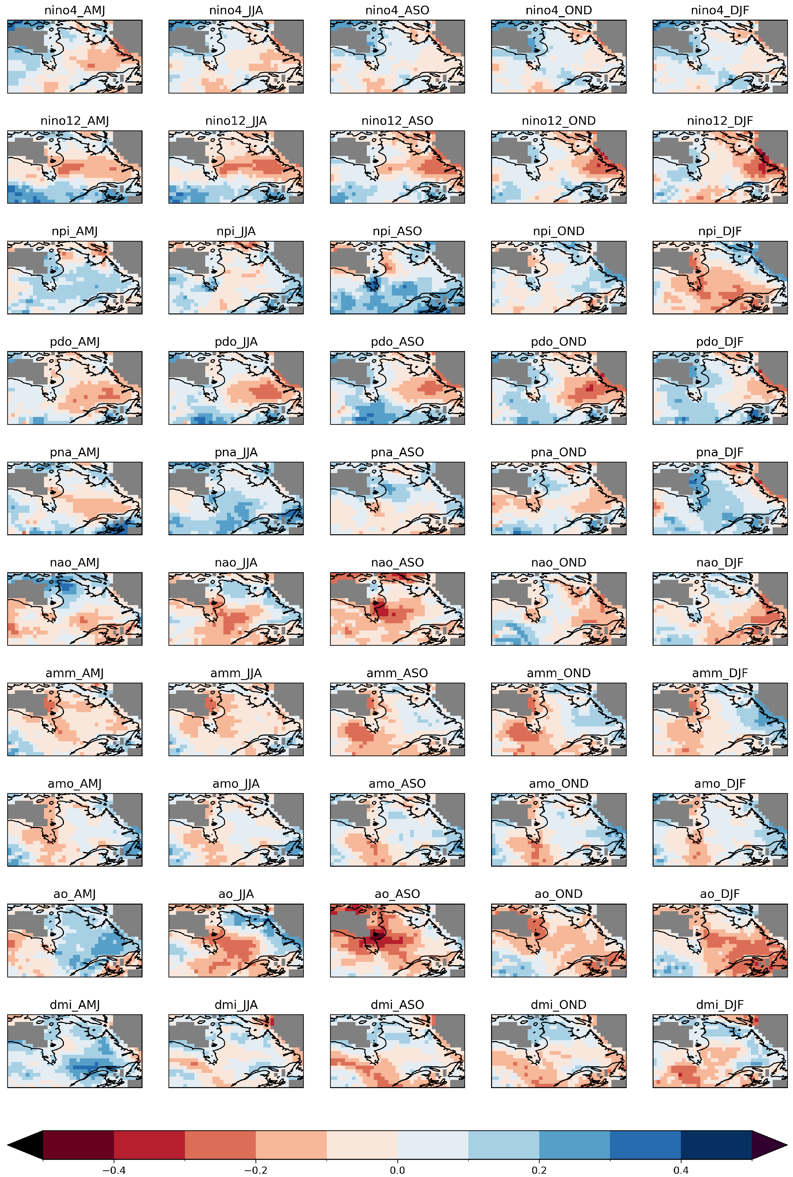
4.1. Climate Indices as Predictands

As the model concept is based on the dependency of wind speed standardized anomalies on climate indices, Figure 2 shows the correlations between each climate index considered for different seasons leading up to the forecast season AMJ. The left column shows the correlation with the AMJ season exactly one year before the season AMJ of interest. From there on, we follow the seasons JJA, ASO, OND, and DJF.

Going through the indices, different intensities of signals can be observed. Overall, the indices NINO12, PDO, NAO, and AO provide the highest values correlations, indicating high predictive power. The areas with the overall highest correlations throughout the indices are the northeastern coastal area, the central area, the eastern area, and the southwestern area. It becomes clear that a different correlation pattern can be identified for each index.

The first illustrated index, NINO4, yields a high correlation for some grid points, especially in the AMJ season for the coastal region and relatively stable prediction zones throughout the seasons. The second index, NINO12, shows an overall higher correlation than NINO4, resulting in correlations ranging lower than −0.2 and higher than 0.3 in the southwestern area for AMJ and JJA and northeastern costal area in ASO, OND, and DJF. The NPI shows highest correlations in the DJF and ASO seasons and a generally large area of consistent positive correlation for DJF, as well as negative for the ASO season. The PDO index shows a strong correlation with the northeastern coastal area in JJA and OND. It also indicates a correlation in the central southern region, most significant in the JJA and ASO seasons. PNA shows weaker overall correlations, with some stronger signals in the central and eastern regions in JJA and the coastal regions of Hudson Bay in DJF. The NAO index indicates a strong correlation for the ASO season in the northwestern area of the examined area. The same area shows a strong negative correlation in the ASO season, expanding across the northern edge of the area, also featuring a very central area. The AMM index correlation displays a comparatively high signal for a distinct area in northeastern Ontario. It also has a correlation with the eastern coast of Newfoundland and Labrador. The AO index provides strong correlation patterns for the southeastern section of the map in DJF and for the northwestern section in ASO.

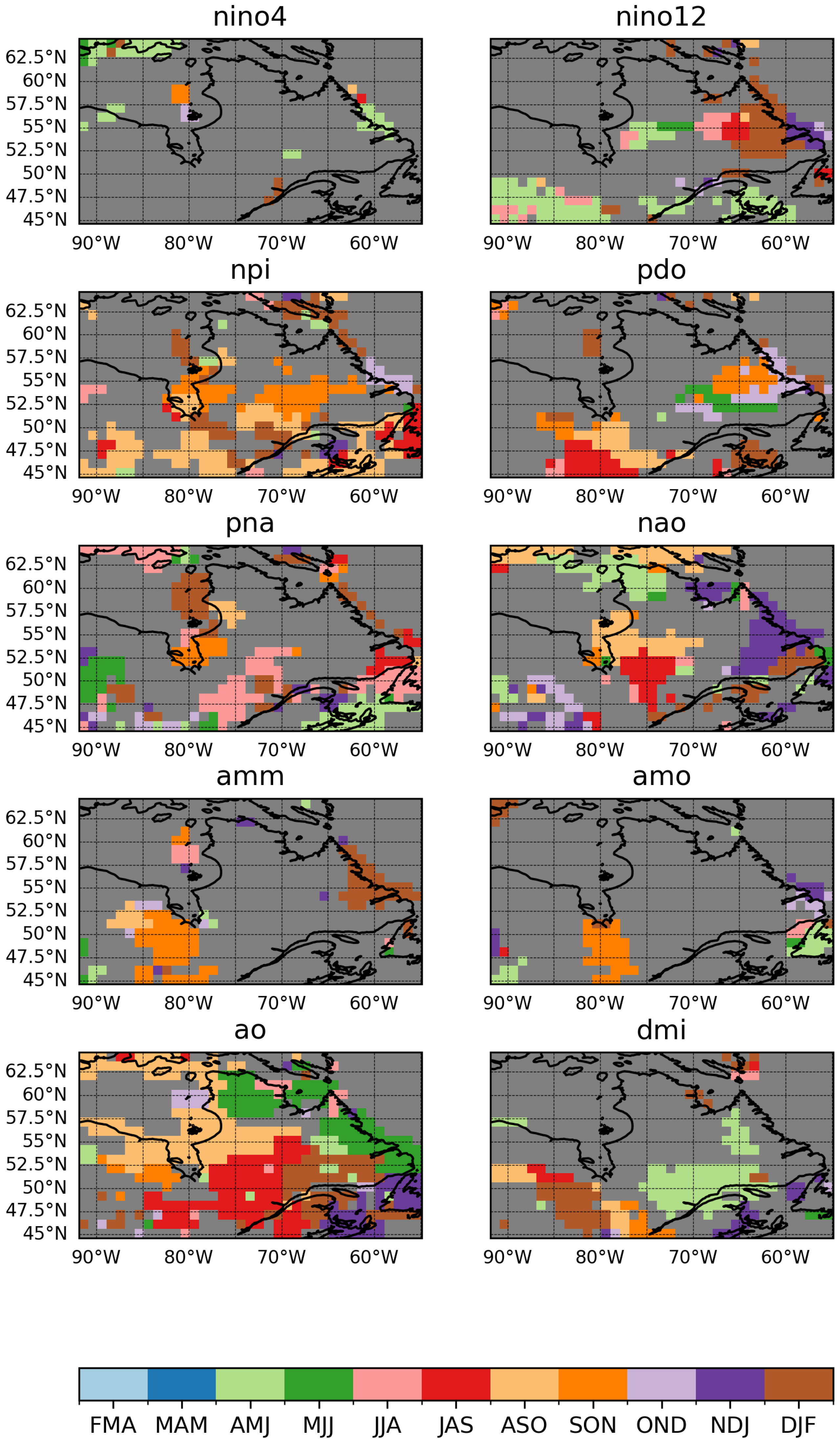
4.2. Season Selection

In order to further assess the most relevant season for the prediction process, as well as the result of selected indices, Figure 3 shows the highest correlated seasons for each of the individual indices. In this case, all correlated seasons with overlap are considered, resulting in a total of 11 seasons leading up to AMJ.

When looking at the seasons selected for the forecast, results differ vastly between indices and areas. Initially, it can be stated that NINO4, as well as AMO were the two indices with the fewest overall gridpoints selected, only covering small groups of used seasons for the northern and coastal parts in the case of NINO4 and eastern coastal parts, as well as southern central part for AMO, respectively. Both of these indices indicate a prominent selection of the ASO, as well as the AMJ season. The indices NINO12, PDO, AMM, and DMI show a greater contribution to forecasts made with a diverse selection of seasons. For NINO12 and DMI, the AMJ and DJF seasons are featured most prominently, whereas PDO shows a diverse mix of selected seasons. AMM shows the most frequent use of the SON and DJF season. Additionally, the indices NPI, NAO, PNA, and AO show the overall fullest selection coverage. The areas covered bear resemblance to each other, being aligned in the northeast coastal area, in the eastern to central southern areas, and in dispersed central coverage. NPI and AO show significant use of the ASO season, with AO’s large areas of different seasons used standing out. PNA and NAO show dispersed use of various seasons.

Overall, the Figure emphasizes the high variability of seasonal correlation in terms of spatial distribution and season selection. The complexity of correlation emphasizes the importance of a straightforward input variable selection approach.

4.3. Sets of Hyperparameters

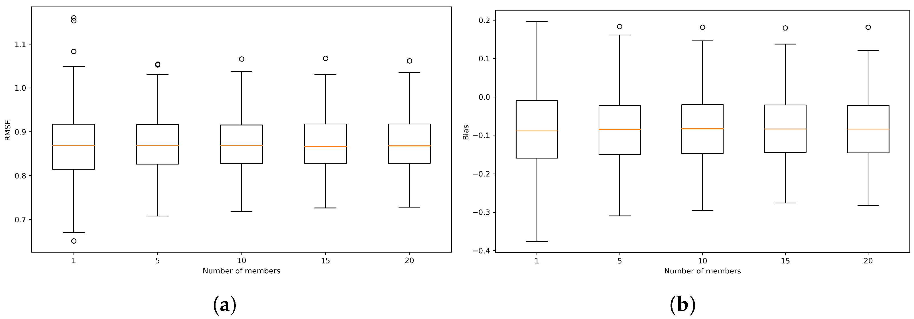
Four different sets of hyperparameters were run in the configured model. The sets differ in terms of the number of units in the hidden layer and the regularization rate. A summary of different configurations is provided in

Table 2. Overview of different sets of hyperparameters trained, showing spatial mean values of RMSE and bias.

Regularization	Units	RMSE	Bias
${10}^{-2}$	1	0.868	−0.084
${10}^{-5}$	1	0.871	−0.084
${10}^{-2}$	3	0.893	−0.087
${10}^{-5}$	3	0.924	−0.088

below, along with the overall mean spatial RMSE and bias values.

In addition, Figure 4 shows box-plots of the RMSE, as well as the bias spatial distribution of the different sets of hyperparameters.

As shown in the box-plots, the first set of hyperparameters, with a regularization rate of ${10}^{-2}$ and 1 unit in the hidden layer, performs best with an average RMSE of 0.868. Reducing regularization to ${10}^{-5}$ does not show a significant change in RMSE. The third combination, with 3 units and a regularization of ${10}^{-2}$, results in an increase in RMSE in most of the grid points. The last set—3 units and a lower regularization of ${10}^{-5}$—features a further RMSE increase, with a significantly wider spread of the 25th and 75th percentiles.

In terms of bias, it becomes clear that the four sets of hyperparameters feature a slight negative bias. The first two configurations perform very similarly, and configurations 3 and 4 show a slight negative shift of the overall distribution. However, when comparing the median bias of the configurations, it becomes clear that the value is very much consistent throughout the varying configurations.

In summary, it can be stated that a simple model consisting of just one unit in the hidden layer and a higher regularization of ${10}^{-2}$ in this case outperforms the other three. This indicates that a simple model design is a better choice than a more complex model. Thus, the first combination of hyperparameters is selected for discussion in the following sections. Running additional sets of hyperparameters could prove valuable; for instance, lower convergence tolerance values could also be tested.

4.4. Ensemble Size

As part of the analysis, the effect of ensemble size on error and bias spatial distribution was examined. The results for the first hyperparameter configuration are displayed as box-plots in Figure 5.

The figure shows the changes in the RMSE and Bias distributions depending on the use of 1, 5, 10, 15, or 20 members in the ensemble. As the box-plots indicate, the size of the ensemble had a small impact on the median values of both RMSE and bias using the selected set of hyperparameters. However, there is a clear narrowing of both metrics distributions from a single model to a five-member ensemble, indicating a decrease in the error and bias spatial variability. Moreover, there is a slight narrowing of the 25th and 75th percentiles as the number of members increases.

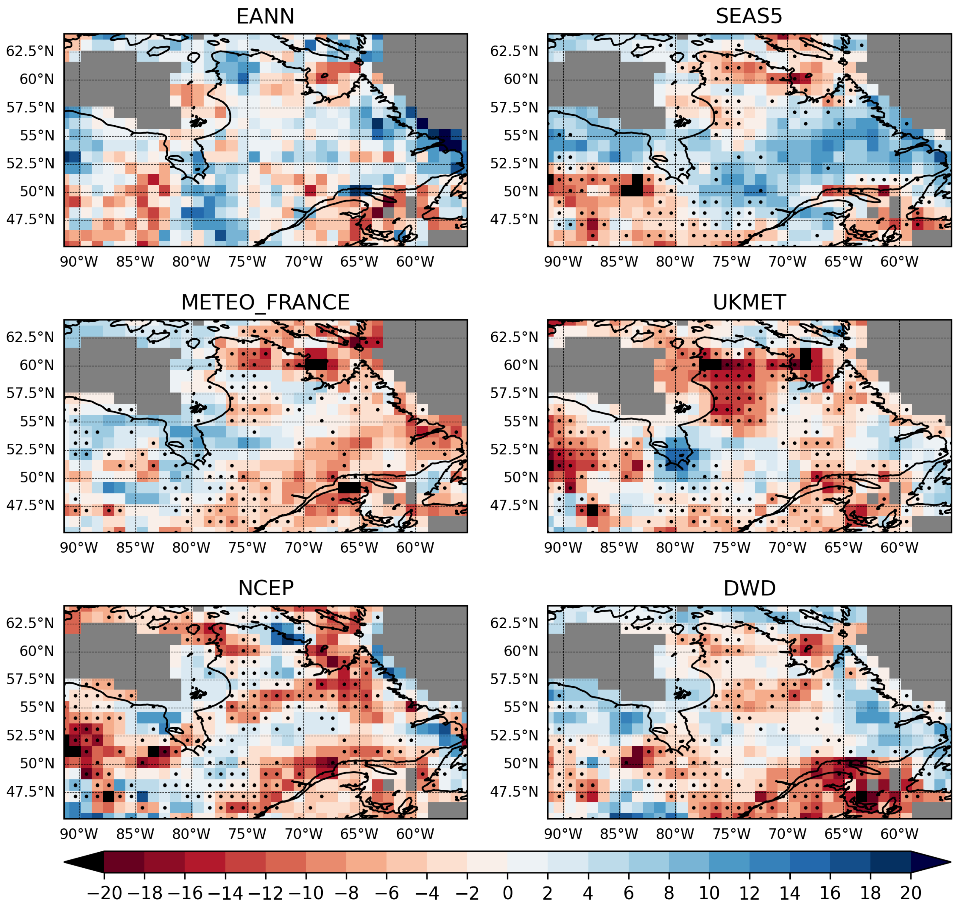
4.5. Model Comparison

In order to assess the performance of the built EANN model, a comparison was made with the state-of-the-art seasonal forecasting models SEAS5, UKMET, NCEP, METEO-France, and DWD. For comparison, the RMSESS was calculated in relation to climatology (Equation (5)) for all models and is illustrated in Figure 6.

To assess whether the observed differences in performance between the EANN and the dynamical models are statistically significant, a paired t-test was performed on the RMSESS values at each grid point. This adds robustness to the model comparison by identifying areas where EANN improvements are unlikely to be due to random variation. Especially for SEAS5, UKMET, and DWD, in the majority of squares where the EANN model outperforms the dynamical model, it does so at the 90% confidence level of the paired t-test.

Initially, it becomes clear that the comparison of the EANN model with SEAS indicates a similar range of results, varying in performance depending on the region examined. The relative accuracy of SEAS5 ranges from −10% to 12%, whereas the EANN performance ranges from −10% to 14%. SEAS5 reaches a relative accuracy greater than 10% in two points in the very northwest sub-region of the selected area. Overall, both models perform well in the central-west, central-south, and central-east regions. SEAS5 outperforms EANN in the north and south of Hudson Bay and in the very central area of the selected region. The EANN has better performance in the southernmost region, especially in southern Quebec (between 80 W and 65 W) and southeastern Newfoundland and Labrador (eastward of 60 W), beating climatology by up to 13% and outperforming all of the compared models. For this region, the majority of squares has a significantly higher RMSESS than the dynamical models at the 90% confidence level. Climatological forecasts outperform the considered models in the southwest of the examined region, east of Hudson Bay, and along the Hudson Strait. In these regions, the reduced EANN performance is due to the reduced selection of indices (Figure 3). An additional reason for the lower performance of the EANN model in the northern Quebec area could be the high variability of annual wind speeds, with an existing and projected overall increase, especially in the area of Nunavik [56]. When considering the models UKMET, NCEP, METEO-France, and DWD, it becomes clear that the models feature different zones of stronger and weaker performances. Whilst UKMET and NCEP indicate a weaker performance ranging from −8% to more than −16% compared to climatology in nothern Ontario, METEO-France and DWD perform comparitively well, outperforming climatology by up to 8%, which is also a better performance than the constructed EANN model. Overall, the performance of the last four models is notably inferior to that of the SEAS and EANN models, thereby supporting the study conducted and highlighting the potential benefits of incorporating a climate index-based forecasting method into an enhanced multi-model ensemble.

This study demonstrates a correlation between climate indices and wind speeds. In order to assess the influence of the different indices, it is of interest to determine which single index or combination of indices produces the strongest results. A well-performing area, such as that east of the twin islands in the southern Hudson Bay at 53° N 79° W, uses the indices NPI, PNA, NAO, and AO. The strongest corresponding correlations are above 0.3 for NPI and below −0.2 for NAO, indicating that those two indices are important predictors for this area. Another strong performance area (Figure 6) east of the Akami–Uapishk–KakKasuak-Mealy Mountains National Park Reserve, ranging from 54° N, 55° W to 56° N, 58° W, is forecast based on NINO12, NPI, PDO, PNA, NAO, AMM, AMO, and AO (Figure 3). When considering the level of correlation, it becomes clear that these indices also show comparably high correlation values, ranging above and below 0.2 and −0.2, respectively (Figure 2). A contributing factor to the model’s good performance is likely the use of NAO winter season indices, as Ouarda and Charron [26] found NAO to have a significant impact on wind speed distributions in eastern Canada during winter months. To assess whether the performance of the model is more dependent on the level of correlation versus the number of predictands, it is interesting to consider the weakly performing area in the very northeast of the case study. Only NINO4 and PDO have significant correlations with the wind speed ranging between 0.2 and −0.2, highlighting the influence of the number of predictands, as well as the level of correlation. Moreover, this also provides information on the predictive power of these two indices as, for instance, NINO4, overall, shows low correlation values for the entire area.

The results suggest that the indices NAO, AO, and NPI have strong predictive power. The season with the most predictive power for the area selected is SON, followed by the subsequent season ASO, indicating high predictive power throughout the August–November months.

Figure 7 shows the spatial average $RMSES{S}_{dyn}$, comparing the EANN performance with dynamical models over the study area. The EANN outperforms most dynamical models, except SEAS5. However, wide error bars indicate substantial variability across the test years.

Another aspect to consider is the varying quality of ERA5 reanalysis data across the case study region. ERA5 wind data are most accurate for flat and sea-level sites with relatively homogeneous land cover [57], whereas heterogeneous land cover and complex topography, such as those found in northeastern Canada, can reduce data reliability. These limitations likely contribute to the reduced performance of the EANN model in such areas, as the underlying input data may not fully capture local wind variability. Future work could explore incorporating higher-resolution datasets or downscaling techniques to better represent complex terrain and land cover variability, as well as testing the model across different geographic regions to evaluate its robustness.

5. Conclusions

Reliable forecasting is essential for the successful implementation of wind energy in the power system and effective scheduling. Modern approaches feature a variety of standalone data-based models, as well as hybrid models consisting of physical and data-driven models for different time horizons. Seasonal forecasting is often used to obtain a better overall idea of wind patterns and capacities. The models in place to provide seasonal forecasts are based on atmospheric and land surface conditions, as well as numerical weather prediction models. While teleconnection-based forecasts have been widely used for climate variables such as precipitation and temperature, their application to wind speed forecasting remains relatively underexplored. This study demonstrates the potential of forecasting wind speeds using correlated climate indices, achieving competitive results compared to current numerical climate prediction models backed by a paired t-test. In terms of $RMSES{S}_{dyn}$ the proposed model outperforms the compared dynamical model, with an exception of SEAS5. The results indicate that a simple ensemble ANN configuration—comprising one hidden unit, a regularization rate of ${10}^{-2}$, and 20 members—yields robust performance, with an overall mean RMSE of 0.868 and a bias of −0.084. This configuration slightly outperforms alternatives with lower regularization and shows a significant improvement over more complex settings. The proposed EANN approach offers practical advantages for operational forecasting due to its ease of implementation and lower computational cost relative to dynamical models. This study contributes to ongoing efforts toward more accurate wind speed forecasting by introducing a novel climate index-based methodology.

Looking ahead, testing this model in different geographic regions would help us to understand how well it performs under varied climate and terrain conditions. There is also potential in exploring hybrid models that combine the ensemble ANN with newer techniques like transformer architectures or probabilistic forecasting frameworks. Additionally, conducting more thorough hyperparameter tuning, including adaptive learning rates, could further boost model performance and reliability. These steps would help move seasonal wind forecasting forward and support the growing role of renewable energy.

References

1. CanREA. Canadian Renewable Energy Association: Wind Energy; CanREA: Ottawa, ON, Canada, 2023. [Google Scholar]
2. Dehghani-Sanij, A.R.; Al-Haq, A.; Bastian, J.; Luehr, G.; Nathwani, J.; Dusseault, M.B.; Leonenko, Y. Assessment of current developments and future prospects of wind energy in Canada. Sustain. Energy Technol. Assess. 2022, 50, 101819. [Google Scholar] [CrossRef]
3. Hanifi, S.; Liu, X.; Lin, Z.; Lotfian, S. A critical review of wind power forecasting methods—Past, present and future. Energies 2020, 13, 3764. [Google Scholar] [CrossRef]
4. WMO. Guidance on Operational Practices for Objective Seasonal Forecasting; WMO: Geneva, Switzerland, 2020. [Google Scholar]
5. Weisheimer, A.; Befort, D.J.; MacLeod, D.; Palmer, T.; O’Reilly, C.; Strømmen, K. Seasonal forecasts of the twentieth century. Bull. Am. Meteorol. Soc. 2020, 101, E1413–E1426. [Google Scholar] [CrossRef]
6. Pryor, S.C.; Barthelmie, R.J.; Bukovsky, M.S.; Leung, L.R.; Sakaguchi, K. Climate change impacts on wind power generation. Nat. Rev. Earth Environ. 2020, 1, 627–643. [Google Scholar] [CrossRef]
7. Ouyang, T.; Zha, X.; Qin, L.; He, Y.; Tang, Z. Prediction of wind power ramp events based on residual correction. Renew. Energy 2019, 136, 781–792. [Google Scholar] [CrossRef]
8. Potter, C.W.; Negnevitsky, M. Very short-term wind forecasting for Tasmanian power generation. IEEE Trans. Power Syst. 2006, 21, 965–972. [Google Scholar] [CrossRef]
9. Candy, B.; English, S.J.; Keogh, S.J. A Comparison of the impact of QuikScat and WindSat wind vector products on met office analyses and forecasts. IEEE Trans. Geosci. Remote Sens. 2009, 47, 1632–1640. [Google Scholar] [CrossRef]
10. Tascikaraoglu, A.; Uzunoglu, M. A review of combined approaches for prediction of short-term wind speed and power. Renew. Sustain. Energy Rev. 2014, 34, 243–254. [Google Scholar] [CrossRef]
11. Yan, J.; Ouyang, T. Advanced wind power prediction based on data-driven error correction. Energy Convers. Manag. 2019, 180, 302–311. [Google Scholar] [CrossRef]
12. Naizghi, M.S.; Ouarda, T.B. Teleconnections and analysis of long-term wind speed variability in the UAE. Int. J. Climatol. 2017, 37, 230–248. [Google Scholar] [CrossRef]
13. González-Sopeña, J.; Pakrashi, V.; Ghosh, B. An overview of performance evaluation metrics for short-term statistical wind power forecasting. Renew. Sustain. Energy Rev. 2021, 138, 110515. [Google Scholar] [CrossRef]
14. Kim, Y.; Hur, J. An ensemble forecasting model of wind power outputs based on improved statistical approaches. Energies 2020, 13, 1071. [Google Scholar] [CrossRef]
15. Soman, S.S.; Zareipour, H.; Malik, O.; Mandal, P. A review of wind power and wind speed forecasting methods with different time horizons. In Proceedings of the North American Power Symposium 2010, Arlington, TX, USA, 26–28 September 2010; IEEE: Piscataway, NJ, USA, 2010; pp. 1–8. [Google Scholar] [CrossRef]
16. Khazaei, S.; Ehsan, M.; Soleymani, S.; Mohammadnezhad-Shourkaei, H. A high-accuracy hybrid method for short-term wind power forecasting. Energy 2022, 238, 122020. [Google Scholar] [CrossRef]
17. Woldesellasse, H.; Marpu, P.R.; Ouarda, T.B. Long-term forecasting of wind speed in the UAE using nonlinear canonical correlation analysis (NLCCA). Arab. J. Geosci. 2020, 13, 962. [Google Scholar] [CrossRef]
18. Bentsen, L.Ø.; Warakagoda, N.D.; Stenbro, R.; Engelstad, P. Spatio-temporal wind speed forecasting using graph networks and novel Transformer architectures. Appl. Energy 2023, 333, 120565. [Google Scholar] [CrossRef]
19. Sarkar, M.R.; Anavatti, S.G.; Dam, T.; Pratama, M.; Al Kindhi, B. Enhancing wind power forecast precision via multi-head attention transformer: An investigation on single-step and multi-step forecasting. In Proceedings of the 2023 International Joint Conference on Neural Networks (IJCNN), Gold Coast, Australia, 18–23 June 2023; IEEE: Piscataway, NJ, USA, 2023; pp. 1–8. [Google Scholar] [CrossRef]
20. Huang, S.; Yan, C.; Qu, Y. Deep learning model-transformer based wind power forecasting approach. Front. Energy Res. 2023, 10, 1055683. [Google Scholar] [CrossRef]
21. Watson, S.; Landberg, L.; Halliday, J. Application of wind speed forecasting to the integration of wind energy into a large scale power system. IEE Proc.-Gener. Transm. Distrib. 1994, 141, 357–362. [Google Scholar] [CrossRef]
22. Costa, A.; Crespo, A.; Navarro, J.; Lizcano, G.; Madsen, H.; Feitosa, E. A review on the young history of the wind power short-term prediction. Renew. Sustain. Energy Rev. 2008, 12, 1725–1744. [Google Scholar] [CrossRef]
23. Giebel, G.; Brownsword, R.; Kariniotakis, G.; Denhard, M.; Draxl, C. The State-of-the-Art in Short-Term Prediction of Wind Power: A Literature Overview; DTU Orbit: Kongens Lyngby, Denmark, 2011. [Google Scholar] [CrossRef]
24. Palmer, T.N. The economic value of ensemble forecasts as a tool for risk assessment: From days to decades. Q. J. R. Meteorol. Soc. A J. Atmos. Sci. Appl. Meteorol. Phys. Oceanogr. 2002, 128, 747–774. [Google Scholar] [CrossRef]
25. Zhang, Y.; Wang, J.; Wang, X. Review on probabilistic forecasting of wind power generation. Renew. Sustain. Energy Rev. 2014, 32, 255–270. [Google Scholar] [CrossRef]
26. Ouarda, T.B.; Charron, C. Non-stationary statistical modelling of wind speed: A case study in eastern Canada. Energy Convers. Manag. 2021, 236, 114028. [Google Scholar] [CrossRef]
27. Lam, R.; Sanchez-Gonzalez, A.; Willson, M.; Wirnsberger, P.; Fortunato, M.; Alet, F.; Ravuri, S.; Ewalds, T.; Eaton-Rosen, Z.; Hu, W.; et al. Learning skillful medium-range global weather forecasting. Science 2023, 382, 1416–1421. [Google Scholar] [CrossRef]
28. Alexiadis, M.; Dokopoulos, P.; Sahsamanoglou, H. Wind speed and power forecasting based on spatial correlation models. IEEE Trans. Energy Convers. 1999, 14, 836–842. [Google Scholar] [CrossRef]
29. Corotis, R.B.; Sigl, A.B.; Cohen, M.P. Variance analysis of wind characteristics for energy conversion. J. Appl. Meteorol. Climatol. 1977, 16, 1149–1157. [Google Scholar] [CrossRef]
30. Giebel, G.; Landberg, L.; Badger, J.; Sattler, K. Using Ensemble Forecasting for Wind Power; OSTI: Oak Ridge, TN, USA, 2003.
31. Ti, Z.; Deng, X.W.; Zhang, M. Artificial Neural Networks based wake model for power prediction of wind farm. Renew. Energy 2021, 172, 618–631. [Google Scholar] [CrossRef]
32. Wu, H.; Meng, K.; Fan, D.; Zhang, Z.; Liu, Q. Multistep short-term wind speed forecasting using transformer. Energy 2022, 261, 125231. [Google Scholar] [CrossRef]
33. Lipu, M.H.; Miah, M.S.; Hannan, M.; Hussain, A.; Sarker, M.R.; Ayob, A.; Saad, M.H.M.; Mahmud, M.S. Artificial intelligence based hybrid forecasting approaches for wind power generation: Progress, challenges and prospects. IEEE Access 2021, 9, 102460–102489. [Google Scholar] [CrossRef]
34. Singh, P.K.; Singh, N.; Negi, R. Wind power forecasting using hybrid ARIMA-ANN technique. In Ambient Communications and Computer Systems: RACCCS-2018; Springer: Singapore, 2019; pp. 209–220. [Google Scholar] [CrossRef]
35. Yang, L.; Sun, Z.; Smith, T. Graph neural networks for multi-site wind forecasting using spatially-aware modeling. Energy AI 2024, 10, 100222. [Google Scholar]
36. Oskarsson, J.; Brown, C.; Lee, W. Graph-EFM: Probabilistic ensemble forecasting of wind using graph neural networks. Renew. Sustain. Energy Rev. 2024, 185, 113714. [Google Scholar]
37. Price, I.; Sanchez-Gonzalez, A.; Alet, F.; Andersson, T.R.; El-Kadi, A.; Masters, D.; Ewalds, T.; Stott, J.; Mohamed, S.; Battaglia, P.; et al. Probabilistic weather forecasting with machine learning. Nature 2025, 637, 84–90. [Google Scholar] [CrossRef]
38. Kent, T.; Saha, S.; MacLachlan, C. Seasonal forecast skill using large-scale climate representations in ACE2. Q. J. R. Meteorol. Soc. 2025; in press. [Google Scholar]
39. Kapica, J.; Canales, F.A.; Jurasz, J. Global atlas of solar and wind resources temporal complementarity. Energy Convers. Manag. 2021, 246, 114692. [Google Scholar] [CrossRef]
40. Zhao, C.; Brissette, F. Impacts of large-scale oscillations on climate variability over North America. Clim. Chang. 2022, 173, 4. [Google Scholar] [CrossRef]
41. Statistics Canada. Electric Power Generation, Monthly Generation by Type of Electricity; Statistics Canada: Ottawa, ON, Canada, 2024.
42. Wilks, D.S. Statistical Methods in the Atmospheric Sciences; Academic Press: Cambridge, MA, USA, 2011; Volume 100. [Google Scholar]
43. NOAA. Climate Indices: Monthly Atmospheric and Ocean Time Series; NOAA: Washington, DC, USA.
44. Johnson, S.J.; Stockdale, T.N.; Ferranti, L.; Balmaseda, M.A.; Molteni, F.; Magnusson, L.; Tietsche, S.; Decremer, D.; Weisheimer, A.; Balsamo, G.; et al. SEAS5: The new ECMWF seasonal forecast system. Geosci. Model Dev. 2019, 12, 1087–1117. [Google Scholar] [CrossRef]
45. Doblas-Reyes, F.J.; García-Serrano, J.; Lienert, F.; Biescas, A.P.; Rodrigues, L.R. Seasonal climate predictability and forecasting: Status and prospects. Wiley Interdiscip. Rev. Clim. Chang. 2013, 4, 245–268. [Google Scholar] [CrossRef]
46. Alessandrini, S.; Sperati, S.; Pinson, P. A comparison between the ECMWF and COSMO Ensemble Prediction Systems applied to short-term wind power forecasting on real data. Appl. Energy 2013, 107, 271–280. [Google Scholar] [CrossRef]
47. Leung, L.R.; Hamlet, A.F.; Lettenmaier, D.P.; Kumar, A. Simulations of the ENSO hydroclimate signals in the Pacific Northwest Columbia River basin. Bull. Am. Meteorol. Soc. 1999, 80, 2313–2330. [Google Scholar] [CrossRef]
48. Torralba, V.; Doblas-Reyes, F.J.; MacLeod, D.; Christel, I.; Davis, M. Seasonal climate prediction: A new source of information for the management of wind energy resources. J. Appl. Meteorol. Climatol. 2017, 56, 1231–1247. [Google Scholar] [CrossRef]
49. Dave, V.S.; Dutta, K. Neural network based models for software effort estimation: A review. Artif. Intell. Rev. 2014, 42, 295–307. [Google Scholar] [CrossRef]
50. Pinheiro, E.; Ouarda, T.B. Short-lead seasonal precipitation forecast in northeastern Brazil using an ensemble of artificial neural networks. Sci. Rep. 2023, 13, 20429. [Google Scholar] [CrossRef]
51. Shu, C.; Burn, D.H. Artificial neural network ensembles and their application in pooled flood frequency analysis. Water Resour. Res. 2004, 40. [Google Scholar] [CrossRef]
52. Sharkey, A.J. Combining Artificial Neural Nets: Ensemble and Modular Multi-Net Systems; Springer Science & Business Media: London, UK, 2012. [Google Scholar] [CrossRef]
53. Kai, L.; Salamon, P. Neural Network Ensembles. IEEE Trans. Pattern Anal. Mach. Intell. 1990, 12, 993–1001. [Google Scholar] [CrossRef]
54. Breiman, L. Bagging predictors. Mach. Learn. 1996, 24, 123–140. [Google Scholar] [CrossRef]
55. Shu, C.; Ouarda, T.B. Flood frequency analysis at ungauged sites using artificial neural networks in canonical correlation analysis physiographic space. Water Resour. Res. 2007, 43. [Google Scholar] [CrossRef]
56. Jeong, D.I.; Sushama, L. Projected changes to mean and extreme surface wind speeds for North America based on regional climate model simulations. Atmosphere 2019, 10, 497. [Google Scholar] [CrossRef]
57. Gualtieri, G. Reliability of ERA5 reanalysis data for wind resource assessment: A comparison against tall towers. Energies 2021, 14, 4169. [Google Scholar] [CrossRef]
Figure 1. Schematic illustration of the training process.
Energies 18 02975 g001
Figure 2. Seasonal correlation of lagged climate indices with ERA5 data for the AMJ season covering the years 1982–2021.
Energies 18 02975 g002
Figure 3. Seasonal correlation used for prediction for each of the utilized indices.
Energies 18 02975 g003
Figure 4. Comparison of different sets of hyperparameters in terms of (a) RMSE and (b) bias.
Energies 18 02975 g004
Figure 5. Comparison of different numbers of members in terms of (a) RMSE and (b) bias.
Energies 18 02975 g005
Figure 6. Comparison of RMSESS between the EANN and dynamical models. Blue areas indicate regions where the models outperform climatology, while red areas indicate a worse performance than climatology. Black dots indicate where the RMSESS of the EANN is significantly higher than that of the dynamical models at the 90% confidence level.
Energies 18 02975 g006
Figure 7. Median R M S E S S d y n [in %] scorebars computed for the test year. Positive values indicate a better performance of EANN, and negative ones indicate a better performance of the dynamical models. Error bars indicate the 90% confidence interval.
Energies 18 02975 g007