Article

Robust Optimal Power Scheduling for Fuel Cell Electric Ships Under Marine Environmental Uncertainty

1
Hyosung Corporation, 74 Simin-daero, Dongan-gu, Anyang-si 14080, Republic of Korea
2
School of Electrical Engineering, Kookmin University, 77 Jeongneung-ro, Seongbuk-gu, Seoul 02707, Republic of Korea
*
Author to whom correspondence should be addressed.
Energies 2025, 18(11), 2837; https://doi.org/10.3390/en18112837
Submission received: 15 April 2025 / Revised: 14 May 2025 / Accepted: 27 May 2025 / Published: 29 May 2025
(This article belongs to the Special Issue Advancements in Marine Renewable Energy and Hybridization Prospects)

Abstract

:
This paper presents a robust optimization-based approach for voyage and power generation scheduling to enhance the economic efficiency and reliability of electric propulsion ships powered by polymer electrolyte membrane fuel cells (PEMFCs) and battery energy storage systems (BESSs). The scheduling method is formulated considering generation cost curves of PEMFCs with mixed-integer linear programming (MILP) and is extended to a robust optimization framework that accounts for marine environmental uncertainties. The robust optimization approach, implemented via the column-and-constraint generation (C&CG) method, ensures stable operation under various uncertainty scenarios, such as wave speed and direction influenced by wind and tidal currents. To validate the proposed method, a simulation was conducted under realistic operational conditions, followed by a case study comparing the MILP and robust optimization approaches in terms of economic efficiency and reliability. Additionally, the optimization model incorporated degradation costs associated with PEMFCs and BESSs to account for long-term operational efficiency. The case study assessed the performance of both methods under load variation scenarios across different marine environmental uncertainties.

1. Introduction

Recently, the Marine Environment Protection Committee (MEPC) of the International Maritime Organization (IMO) strengthened its greenhouse gas (GHG) emission reduction targets for the global shipping industry. The updated targets aim to reduce GHG emissions by 70% by 2040 compared to 2008 levels and achieve net-zero emissions by 2050 [1]. In response to these stricter regulations, the shipping industry has adopted various eco-friendly technologies and operational strategies to mitigate emissions. Measures such as using low-sulfur fuel and installing emission reduction devices have been implemented, but while these steps contribute to incremental reductions, they remain insufficient to meet long-term targets [2]. A more fundamental solution involves improving the energy efficiency of ships through propulsion system modifications, which has emerged as a critical strategy for reducing fuel consumption.
Electric propulsion systems integrate power from onboard generators and distribute it to propulsion motors and other electrical loads, allowing for flexible and optimal generator operation based on load conditions. This improves energy efficiency while enhancing reliability and survivability by ensuring continued operation in the event of generator failure. Additionally, separating generators from propulsion motors increases design flexibility, enabling the integration of various power sources and energy storage systems (ESSs) [3,4]. To achieve net-zero emissions, transitioning from conventional fossil fuel generators to environmentally friendly power sources is essential. Hydrogen and ammonia fuel engines, fuel cells, and battery energy storage systems are key technologies driving this transition. Among them, fuel cells are considered crucial for both decarbonization and the electrification of ships. They generate electricity through a chemical reaction between hydrogen and oxygen, emitting only pure water as a byproduct, making them an environmentally friendly power source. In fuel-cell-powered ships, internal combustion engines are replaced by propulsion motors driven by electricity generated from fuel cells [5].
Polymer electrolyte membrane fuel cells (PEMFCs) are widely used in various applications, including automobiles and ships, due to their fast startup time, rapid response characteristics, high power density, and efficiency [6]. However, PEMFCs are susceptible to performance degradation under operational conditions such as frequent load fluctuations, startup and shutdown cycles, high-power operation, and low-power operation. These conditions can lead to uneven current distribution, overheating, catalyst degradation, and membrane damage, ultimately reducing reliability and efficiency over time [7]. To address these challenges, integrating battery energy storage systems (BESS) with PEMFCs has gained attention as a way to enhance system stability. BESS helps maintain optimal operating conditions by mitigating stress caused by frequent load variations and startup/shutdown cycles. During peak loads, BESS discharges to prevent excessive loading of PEMFCs, while during low loads, it charges to avoid inefficient low-power operation. The coordinated operation of PEMFCs and BESS improves both efficiency and reliability, playing a crucial role in advancing ship electrification and decarbonization [8].
Several real-world implementations have demonstrated the feasibility of PEMFC/BESS hybrid propulsion systems, with some projects progressing to actual shipbuilding and operation. The Sea Change, launched in August 2021, is the first hydrogen fuel cell-powered vessel in the United States and the world’s first commercial ferry powered by hydrogen fuel cells. It is equipped with a 360 kW PEMFC, a 100 kWh lithium-ion battery, and two 300 kW propulsion motors. When cruising at 12 knots, it can travel approximately 278 km on a single hydrogen tank refill, with a maximum speed of up to 20 knots. The vessel operates by charging the battery during idling or low-speed sailing and utilizing battery power alongside the fuel cell during high-speed operation [9]. In [10], a PEMFC–battery hybrid propulsion system was developed for a 20-m-long sightseeing vessel and demonstrated in the coastal waters of Busan. Its power system consists of a 50 kW PEMFC and a 47 kWh lithium-ion battery, with an operational strategy that varies based on load conditions. Under low loads, the PEMFC operates independently, increasing to full capacity as the load reaches its rated power. Under high load conditions, the PEMFC and ESS coordinate output control, enhancing both stability and operational efficiency.
Building on these advancements, recent studies have proposed strategies to optimize the economic and environmental performance of shipboard power systems. Kanellos et al. [11] introduced a cost- and emission-aware power management system integrating generator scheduling, ESS control, propulsion adjustment, and cold-ironing. Aziz et al. [12] proposed a coordinated control strategy for hybrid ship power systems with multiple PEMFCs and BESS units, combining master–slave and droop control to ensure stability under dynamic load conditions. Fang et al. [13] developed a two-step optimization framework for hybrid ESS operation, simultaneously minimizing fuel costs, emissions, and battery degradation.
In recent years, increasing attention has been paid to the impact of uncertainties in marine environments, such as wind, waves, and unpredictable voyage conditions. In response, various strategies have been proposed to incorporate uncertainty into the operation and scheduling of shipboard power systems. Taheri et al. developed a trip-ahead dispatch strategy for diesel generators to improve energy efficiency under uncertain forecasts [14]. Uncertainty modeling and management have been widely explored with various approaches such as stochastic programming, Bayesian methods, data-driven techniques, and distributionally robust optimization.
Based on these developments, this study adopts robust optimization as the primary method for handling uncertainty. In real-world ship operations, collecting detailed data on marine environmental conditions or fuel consumption behavior is challenging. These constraints limit the applicability of many existing methods. Stochastic programming, for example, relies on accurate probability distributions and requires extensive scenario trees, which leads to exponential model growth and reduces the flexibility for real-time re-optimization [15]. Although data-driven approaches can offer high predictive accuracy, they are effective only when large volumes of high-quality operational data are available, which is often difficult to achieve in maritime settings [16]. Distributionally robust optimization provides additional flexibility in modeling uncertainty, but its performance heavily relies on the careful design of ambiguity sets. If these sets are poorly specified, the resulting solutions may become overly conservative or unrealistically optimistic, requiring caution for practical implementation [17].
In contrast, robust optimization requires only simple uncertainty bounds to produce reliable schedules and demonstrates high computational efficiency. These characteristics make it particularly suitable for shipboard scheduling problems, where both real-time responsiveness and operational robustness are essential, as in the case of this study.
Several recent studies have also applied robust optimization to ship scheduling problems, aiming to address environmental uncertainties in practice. In [18], a two-stage robust optimization model was developed for all-electric ships equipped with diesel generators and multiple BESS units. This model separates pre-voyage generator on/off scheduling from intra-voyage load control and employs sequential battery usage to extend battery life, ensuring robust operation under navigational uncertainties such as waves and wind. In [19], a hybrid AC/DC multi-energy microgrid configuration was proposed, integrating diesel generators, a photovoltaic (PV) system, and a BESS. The authors employed the column-and-constraint generation method, which divides the problem into a master problem for voyage-ahead decisions and a slave problem for worst-case uncertainty scenarios, reducing computational complexity and improving convergence. This approach ensures robust, cost-efficient operation under diverse uncertainties, enhancing the ship’s operational reliability and adaptability.
However, these studies primarily focus on diesel-based hybrid systems or consider PEMFCs as auxiliary power sources. Therefore, when determining operational strategies, they often account only for fuel costs or simplistic degradation costs due to on/off cycles. These approaches overlook the fact that the degradation rate of PEMFCs varies significantly with dynamic load conditions, especially when PEMFCs serve as the main propulsion source in zero-emission ships. A more accurate and detailed degradation model is essential in such cases.
This paper aims to optimize the operation of PEMFC/BESS hybrid ships to improve economic efficiency and reliability while addressing challenges posed by marine environmental uncertainties. The configuration of the PEMFC/BESS hybrid ship is shown in Figure 1, where the arrows indicate the direction of power flow between components.
The key contributions of this work are as follows:
  • An optimal power and voyage scheduling method is developed for PEMFC/BESS hybrid ships operating on coastal round-trip routes. This method optimizes total operational costs by considering fuel costs, degradation costs of fuel cells and BESS, cold-ironing costs, and economically efficient operating speeds.
  • A robust optimization-based scheduling approach is proposed to address uncertainties affecting ship speed in marine environments. This method enables the system to flexibly adapt to unforeseen changes or errors, ensuring stable and reliable operation under varying conditions.
  • A strategy specifically designed for zero-emission ships powered solely by fuel cells is introduced. By leveraging the high efficiency of PEMFCs during low-load operation, this method employs a preplanned schedule covering a range of uncertainty scenarios. It allows multiple PEMFCs to operate concurrently while maintaining each cell within its optimal low-load, high-efficiency region.
The remainder of this paper is structured as follows. Section 2 describes the optimal scheduling methods based on the MILP optimization technique and the robust optimization technique using the column-and-constraint generation (C&CG) method. Section 3 explains the models for the two proposed power generation scheduling methods. Section 4 presents a comparative analysis of the simulation results for these methods. Finally, Section 5 concludes with the findings of the proposed approach.

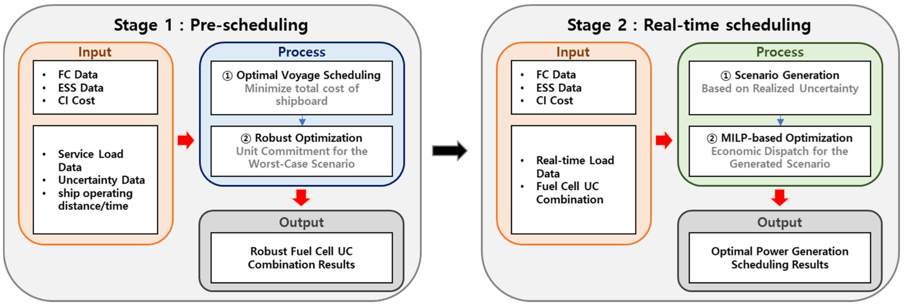
2. Problem Description

Section 2 introduces a two-stage scheduling method for PEMFC/BESS hybrid ships using the mixed-integer linear programming (MILP) optimization technique. The optimization process is divided into two stages, as follows:
  • Stage 1 (Pre-scheduling): Power generation and voyage planning are optimized over predicted load scenarios to produce a unit commitment (UC) plan. This plan defines on-off schedules for PEMFC and BESS units in advance of the voyage.
  • Stage 2 (Real-time scheduling): During ship operation, economic dispatch (ED) follows the UC plan to accommodate actual load fluctuations. Generation outputs are adjusted in real time to track the true power demand.
By combining pre-scheduling with real-time dispatch, this framework minimizes cost and maintains reliable operation for the load profiles it was designed around. However, because it relies on accurate forecasts, it cannot guarantee cost minimization or system reliability under unexpected load variations.
The primary objective of this scheduling method is to minimize operational costs under forecasted load profiles while maximizing economic efficiency. To achieve this, a quadratic fuel consumption cost function is derived from the PEMFC efficiency curve and incorporated into the optimization model. Additionally, degradation costs are included in the objective function to account for performance deterioration of PEMFCs and BESSs.

2.1. Optimal Power Generation Scheduling for PEMFC/BESS Shipboard Power System

Optimal power generation scheduling for a ship aims to minimize operational costs under a given voyage scenario. The costs considered in this study include hydrogen consumption, PEMFC degradation, BESS degradation, and cold-ironing costs [20]. The process begins with collecting input data, such as the PEMFC cost function, BESS specifications, cold-ironing electricity tariffs, and ship load data. Next, the objective function and constraints are defined: the objective function seeks to minimize operational costs, while the constraints ensure power supply–demand balance and adherence to the operational limitations of power generation units.

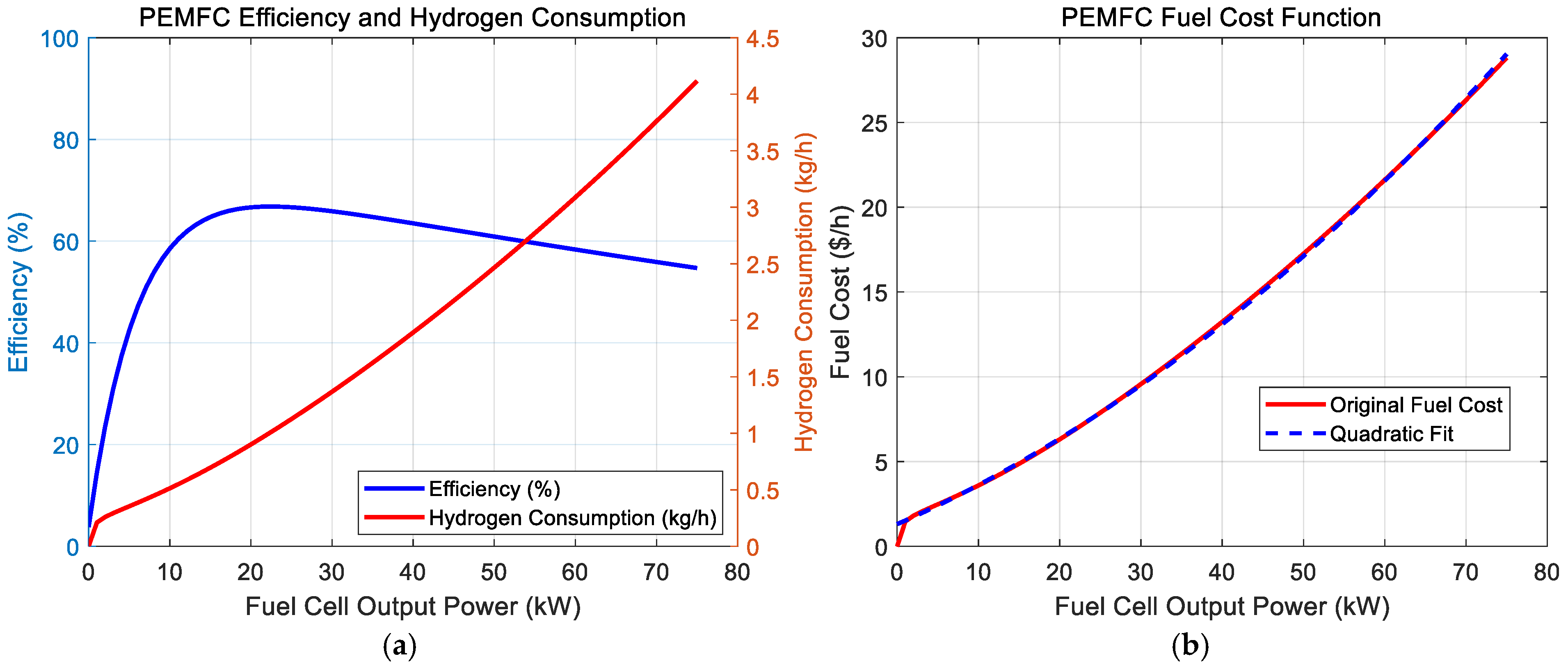
2.1.1. PEMFC Cost Function

For optimal power generation scheduling, the PEMFC fuel cost function is derived from its efficiency curve based on the lower heating value (LHV) of hydrogen. PEMFCs exhibit efficiencies between 45% and 60%, achieving their peak efficiency within a specific output range but decreasing in efficiency as output increases [21]. This differs from conventional diesel and gas turbine generators, which improve in efficiency as they approach their rated capacity.
To accurately model PEMFC fuel consumption, the cost function is formulated using efficiency curve data. The hourly fuel consumption cost, C F C , i t ($/h), is determined at each output level [22] as follows:
η F C S = P F C , i m H 2 H L H V
m H 2 = P F C , i η F C S H L H V = K E m E F C , i
E F C , i = a i P F C , i 2 + b i P F C , i + c i
C F C , i = C H 2 m H 2 = C H 2 K E m E F C , i
where C F C , i ($) represents the PEMFC fuel consumption cost, calculated as the product of the hydrogen price, C H 2 ($/kg), and the mass of consumed hydrogen, m H 2 (kg). The mass of consumed hydrogen is derived from the PEMFC efficiency in Equation (1). P F C , i denotes the PEMFC output power (kW), and H L H V is the lower heating value of hydrogen (kWh/kg). The MATLAB R2024b curve fitting toolbox was used to compute the hydrogen consumption m H 2 (kg) at different points P F C , i (kW) output points based on the efficiency curve in Figure 2a. Additionally, hydrogen consumption was calculated using energy E F C , i , expressed as a quadratic polynomial in Equation (3), along with the conversion factor K E m to convert hydrogen energy into mass. The resulting fuel cost function, depicted in Figure 2b, effectively models PEMFC nonlinear output characteristics, providing key parameters for optimizing energy efficiency while minimizing fuel costs. The fitting performance evaluation for this function is detailed in Appendix A (Table A1).

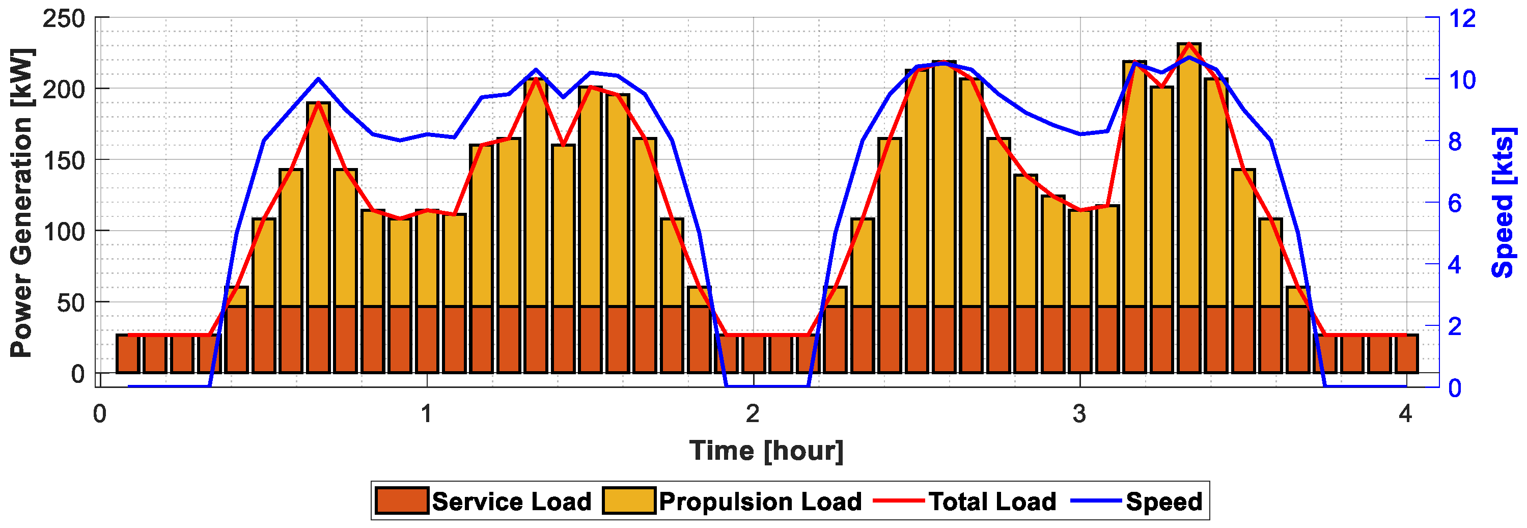
2.1.2. Propulsion Load

A ship’s propulsion load refers to the power consumed by the propulsion propeller, which constitutes a significant portion of total energy consumption. Notably, propulsion load increases proportionally to the cube of the ship’s speed, meaning even small changes in speed have a significant impact on energy consumption. At maximum speed, propulsion load accounts for approximately 90% of the total load, making it a crucial factor in scheduling [23].
To determine the propulsion load, ship speed characteristics are used to model the relationship between speed and fuel consumption. The propulsion load at different speeds is approximated using a cubic polynomial function, formulated as:
P p r o p v = i = 0 3 c i v i = c 3 v 3 + c 2 v 2 + c 1 v + c 0
where c 0 , c 1 , c 2 , and c 3 are derived from speed-specific load data using the MATLAB Curve Fitting Toolbox, as shown in Figure 3. This polynomial approximation serves as essential input data for optimizing power generation scheduling. Appendix A (Table A2) provides the fitting performance evaluation for this approximation.

2.1.3. Voyage Scheduling

A ship’s propulsion load is proportional to the cube of its speed, meaning that even small reductions in high-speed operation can significantly lower fuel costs. Therefore, the optimal voyage and power generation scheduling method for PEMFC/BESS hybrid ships aims to determine an economical operating speed through voyage scheduling, thereby minimizing fuel consumption and operational costs. Voyage scheduling is performed during the first-stage optimization, where ship speed and load data are generated and then used as input for the second-stage economic dispatch (ED) optimization.
As shown in Equation (6), the ship’s operating speed is constrained within predefined minimum and maximum speed limits for each operating mode, preventing excessive acceleration or deceleration. The voyage distance for each time interval is updated based on the previous distance traveled and the current speed, as described in Equation (7). Finally, Equation (8) ensures that the total travel distance remains within specified limits, maintaining an economical and efficient voyage [24].
v m i n t v t v m a x t
D t = D t 1 + v t × t
D m i n t D t D m a x t

2.2. Robust Optimization for PEMFC/BESS Shipboard Power System

The MILP-based optimal power generation scheduling described in Section 2.1 provides an optimized schedule based on predicted load scenarios. However, actual ship operations are influenced by uncertainties in the marine environment, such as wind and waves, which significantly impact propulsion load. These uncertainties can increase fuel consumption and reduce both the feasibility and economic efficiency of pre-determined scheduling results. In other words, optimization based solely on predicted load data may fail to ensure optimal performance in real-world conditions, compromising the reliability of ship operations [25].
To address this challenge, a two-stage optimal scheduling method utilizing robust optimization is proposed. This approach incorporates marine environmental uncertainties to enhance the flexibility and reliability of power generation scheduling. By considering various uncertainty scenarios, the method ensures system stability and minimizes operational costs, even under worst-case conditions.

2.2.1. Robust Optimization

Robust optimization ensures system stability and performance in the presence of uncertainties or external disturbances by maintaining system operation within a defined range. This approach enables flexible adaptation to unforeseen variations while ensuring that solutions remain feasible under any uncertain conditions [19]. The two-stage optimal power generation scheduling method based on robust optimization consists of pre-scheduling before the voyage and real-time scheduling during the voyage. Each phase employs the MILP optimization technique described in Section 2.1, ensuring robust and efficient scheduling throughout the operational cycle. The overall structure of this scheduling approach is illustrated in Figure 4.
In the first stage, pre-scheduling is performed based on predicted load and uncertainty data according to the planned route and voyage schedule. The optimization objective is to minimize operational costs under worst-case scenarios that may arise during operations. Uncertainties such as wind and waves are modeled as load variations caused by speed losses. The optimization determines a UC plan that ensures robust operation even under the most adverse load variations. Since the results account for worst-case scenarios, operational costs tend to be higher, and the power generation configuration is conservatively determined to ensure robustness.
In the second stage, real-time scheduling adapts to uncertainties that arise during actual ship operations. Economic dispatch is performed based on the power generation configuration determined in the first stage. As worst-case scenarios do not always occur, operational costs in this stage are typically lower than those in the first stage. Through these two scheduling stages, PEMFC and BESS outputs are optimized based on real-time load data, minimizing operational costs while ensuring system reliability and economic efficiency.

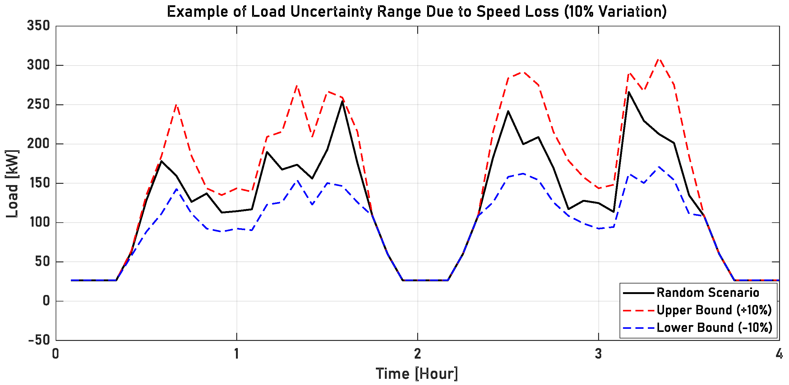
2.2.2. Uncertainty in Marine Environments

Wave height and length, wind speed, and wind direction are the four primary factors contributing to cruising speed losses during ship operations. These factors can cause speed reductions of up to 10% under normal sea conditions [18]. When speed loss occurs, additional power is required to maintain the intended speed. Since a ship’s propulsion load is proportional to the cube of its speed, the increase in load becomes significantly larger as speed increases.
Consequently, speed losses lead to higher fuel consumption and potential delays in operation. In [26], fuel consumption was analyzed under various sea conditions based on operating speed. The results confirmed that as the Beaufort wind scale (BF) increases, fuel consumption rises due to greater wave heights and wind resistance, both of which demand more power to maintain a constant speed. Since propulsion load accounts for approximately 90% of the total energy demand, it is essential to incorporate these factors when designing scheduling methods.
To account for speed losses caused by uncertainties, the propulsion load equation for speed, initially defined in Equation (5), is modified as follows:
  P p r o p v = i = 0 3 c i × v ( v c a l m + Δ v ) i
δ × v c a l m Δ v δ × v c a l m
where v c a l m represents the ship’s speed in calm sea conditions, and Δ v denotes the speed variation due to marine environmental uncertainties. The actual operating speed is the sum of these two values. If speed loss occurs, the propulsion load increases; conversely, if uncertainties result in a speed increase, the propulsion load decreases.
Equation (10) defines the range of speed uncertainty based on the maximum variation rate, δ , of the nominal speed, a critical factor in determining system robustness. A wider uncertainty range enhances the system’s ability to handle fluctuation but also results in more conservative scheduling outcomes.
As shown in Figure 5, variations in propulsion load due to uncertainties are determined by speed-dependent equations. Since propulsion load is proportional to the cube of speed, even minor speed fluctuations caused by uncertainty can lead to significant nonlinear changes in load. Therefore, accurately modeling marine environmental uncertainties and incorporating them into scheduling methods is crucial for optimizing ship performance and efficiency.

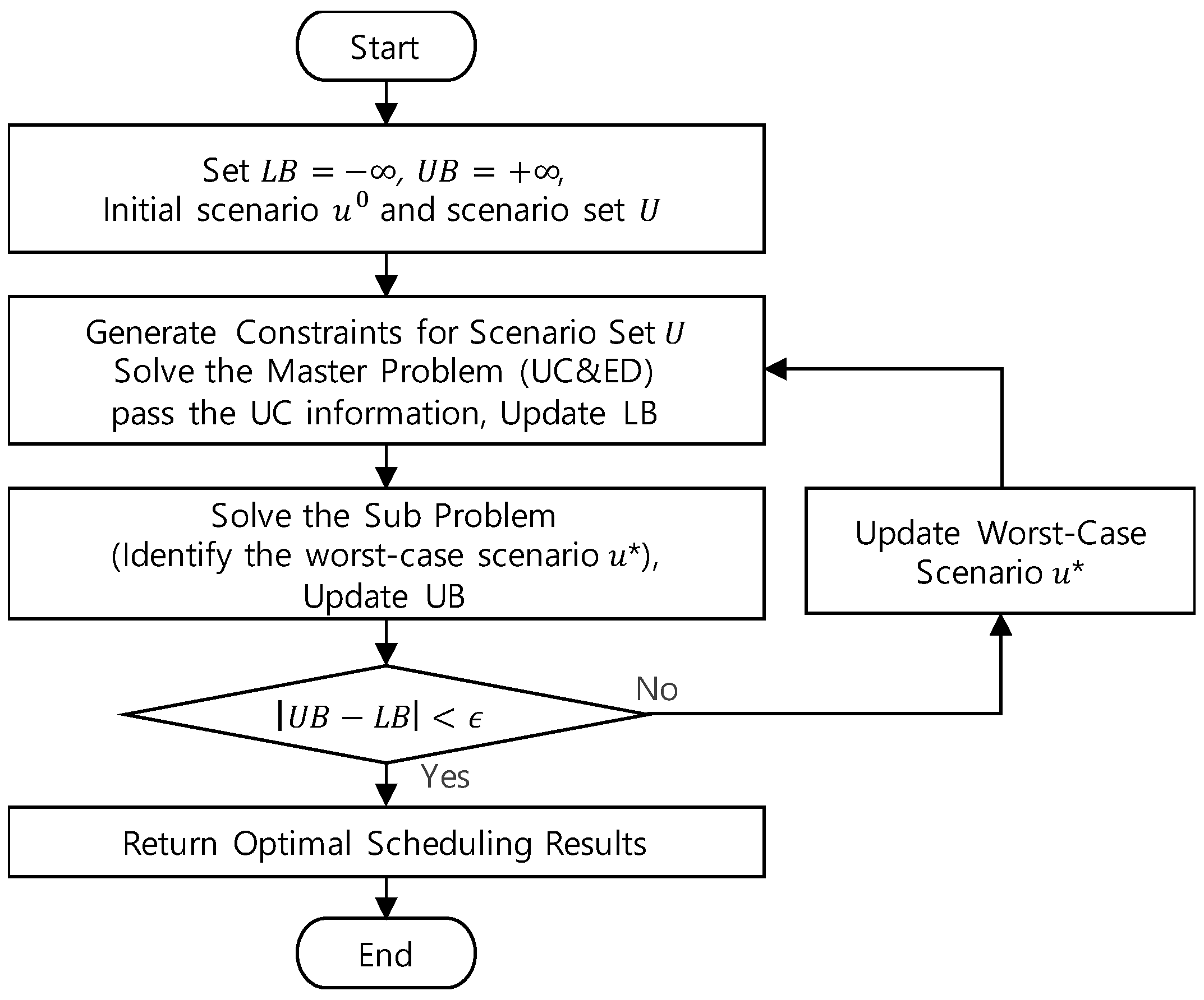
2.2.3. Column-and-Constraint Generation Method

In the two-stage optimal power generation scheduling process based on robust optimization, the first stage identifies the worst-case scenario and derives an optimal scheduling strategy to address it. The second stage adjusts the schedule based on the realization of uncertainties.
Each stage is modeled using MILP or MINLP, depending on the characteristics of the shipboard system. Two-stage robust optimization problems require decision-making that accounts for worst-case scenarios within a defined uncertainty set, enabling more realistic modeling compared to single-stage robust optimization. However, this approach also significantly increases computational complexity. In particular, when the problem includes a two-stage recourse structure, it results in a tri-level optimization formulation, which is extremely challenging to solve [27].
Previously, dual-based cutting plane methods such as Benders decomposition (Benders-dual cutting plane) were commonly used. However, these methods present challenges in implementation complexity and convergence stability due to their reliance on adding constraints to the master problem using the dual solution of the subproblem [28]. A more effective approach to overcoming these limitations is the C&CG method. Unlike dual-based methods, the C&CG method does not rely on dual solutions but instead directly generates variables and constraints in the primal space through an iterative approach, making it more intuitive and computationally efficient.
The mathematical formulation of the two-stage robust optimization problem using the C&CG method is presented in [27,28]:
m i n y Y c T y + m a x u U m i n x X y , u d T x
where y represents the first-stage decision variables, and x denotes the second-stage recourse variables determined after the uncertainty u U is revealed. This structure captures a two-stage robust optimization problem, where the outer minimization determines the first-stage decisions, and the inner max–min formulation identifies the worst-case second-stage cost under uncertainty. Since solving this min–max–min structure directly is computationally infeasible, the C&CG method approximates the solution iteratively using a Master–Subproblem framework.
m i n { y , η } { c T y + η }
η d T x i ,   i = 1 , , k
x i X y , u i ,   i = 1 , , k
Equation (12) represents the Master Problem, which optimizes the first-stage decision based on the worst-case scenarios identified so far. Here, η is an auxiliary variable that provides an upper bound on the worst-case second-stage cost. The Master Problem is constrained by Equations (13) and (14), ensuring that, for all previously identified worst-case scenarios, the system remains feasible while keeping the second-stage cost within the bound η .
u = a r g max { u U } min { x X ( y , u ) } d T x
Equation (15) represents the Subproblem, which identifies the worst-case scenario given the current first-stage decision y . The worst-case uncertainty u * identified in this step is then added to the Master Problem. By iterating between the Master and Subproblem, the algorithm ensures that the current decision y remains robust under the most adverse conditions. This iterative process continues until convergence is achieved.
Through this approach, the C&CG method efficiently solves the problem over a limited set of scenarios, progressively refining the model by identifying new worst-case scenarios. This ensures both computational efficiency and solution accuracy.
In this study, the C&CG method is applied to the power scheduling problem of a fuel cell-based electric propulsion ship. This problem involves both discrete decision variables and continuous recourse variables. Moreover, fuel consumption and operational costs are highly sensitive to prediction errors, necessitating a robust and precise optimization approach.
As illustrated in Figure 6, the C&CG method consists of:
  • A Master Problem, which optimizes scheduling based on a predefined set of uncertainty scenarios.
  • A Subproblem, which identifies and adds new worst-case scenarios to the set [29].
Initially, the scenario set is constructed based on predicted load scenarios. The C&CG algorithm then iteratively solves a master problem and a subproblem, progressively adding columns and constraints to incorporate newly identified uncertainty scenarios. Specifically, the master problem optimizes scheduling over the current scenario set, determining the lower bound (LB) of the objective function based on the scenarios considered thus far.
Next, the subproblem evaluates the master solution and identifies the worst-case scenario—i.e., the scenario that results in the highest cost (or objective value) under all possible uncertainties for the given generator configuration. This worst-case scenario is added to scenario set U, thereby defining the upper bound (UB). With each newly added scenario, the master problem is re-optimized with updated columns and constraints, ensuring that the LB increases (or remains unchanged) while the UB decreases (or remains unchanged) at each iteration.
In this process, the worst-case scenario corresponds to the condition that leads to the highest operational cost given the current generator configuration. If, after re-optimization, the generator configuration remains unchanged, the scenario set is considered complete, and the iteration terminates. However, if the configuration changes, the subproblem is solved again to determine a new worst-case scenario, which is then added to U. Through these iterative steps, the algorithm systematically explores and expands the set of uncertainty scenarios, ultimately deriving a stable and cost-effective solution that accounts for all identified uncertainties.
The C&CG method concludes once the gap between UB and LB is reduced to a predefined threshold ( ϵ ), which balances solution accuracy and computational efficiency. For instance, setting ϵ to approximately 10−2 or 10−3 enables the rapid attainment of a robust optimal solution within an acceptable margin of error. If ε is set too small, computational time may increase excessively, while setting it too large may reduce solution accuracy. Therefore, an appropriate value is selected to simultaneously satisfy both accuracy and computational efficiency. This C&CG-based two-stage robust optimization approach effectively manages highly uncertain problems, such as shipboard power scheduling.

3. Mathematical Description

3.1. Optimal Operation of PEMFC/BESS Shipboard Power System with Voyage Scheduling

3.1.1. Objective

The objective of the optimal power generation scheduling for PEMFC/BESS hybrid ships is to minimize total operational costs. These costs include PEMFC hydrogen consumption, PEMFC degradation, BESS degradation, and cold-ironing expenses. The optimization problem is formulated as the objective function in Equation (16).
Equations (17) and (18) incorporate PEMFC and BESS degradation costs, respectively, to account for performance deterioration due to operation, thereby reducing maintenance and replacement cycles and ensuring long-term reliability and cost-effectiveness. Equation (19) represents the cost incurred from using cold-ironing while docked. Here, T   is the total scheduling time interval, N F C is the number of PEMFC units, and m 1 to m 4 are weighting coefficients in the optimization function.
  min f x = t = 1 T i = 1 N F C m 1 C F C , i t + m 2 C F C , d e g , i t + m 3 C B E S S , d e g t + m 4 C C I t
C F C , d e g , i t = C h i g h , i t + C l o w , i t + C s t a r t u p , i t + C i s o n , i t
C B E S S , d e g t = P B E S S , d s c t C B E S S , d e g η d s c
C C I t = C e l e c t r i c   c h a r g e P C I t
The degradation cost of PEMFCs accounts for key deterioration factors, helping to minimize maintenance and replacement cycles and ensuring long-term system reliability. PEMFC performance degrades over time due to internal voltage drop, which must be maintained within allowable limits for stable operation. Therefore, the degradation cost is calculated based on the allowable voltage drop over the PEMFC’s lifespan [30].
Equations (20)–(23) define degradation costs associated with high-loading operation, low-loading operation, startup actions, and general operating conditions, respectively. Here, C h i g h , i t represents the degradation cost ($) from high-loading operation, C l o w , i t accounts for low-loading operation, and C s t a r t u p , i t represents degradation due to startup operations [30]. Additionally, C i s O n , i t refers to the degradation cost ($) incurred when PEMFC is operating.
C h i g h , i t = α h i g h T h i g h , i t p s t a c k u E O L , F C
C l o w , i t = α l o w T l o w , i t p s t a c k u E O L , F C
C s t a r t u p , i t = α s t a r t p s t a c k u E O L , F C × ξ F C t
C i s O n , i t = p s t a c k T E O L , F C × U F C , i t
where α h i g h and α l o w represent the voltage drop (μV/h) caused by high and low loading, respectively, while α s t a r t represents voltage drop (μV/start) due to startup actions. The parameter u E O L , F C is the maximum allowable voltage drop (μV) over the PEMFC’s lifespan, and p s t a c k is the PEMFC stack cost ($). The terms T h i g h , i t and T l o w , i t are the high and low loading operation times (h), while ξ F C t is a binary variable indicating startup actions.
Degradation due to load variations is modeled as a voltage drop from short-term fluctuations. However, since this scheduling approach considers long time intervals, short-term voltage drops are not explicitly included. Instead, degradation is modeled based on the PEMFC’s target operating time. The term T E O L , F C represents the expected PEMFC lifespan, and U F C , i t indicates whether the FC is operating during a given time interval.
The BESS degradation cost arises during discharge and is calculated based on BESS discharge power and degradation costs. Here, P B E S S , d s c t denotes the BESS discharge power (kW), C E S S , d e g represents BESS degradation cost, and η d s c is BESS discharge efficiency (%) [24].
When the ship is docked, cold-ironing can be used to charge the BESS or supply power to hotel loads. The associated cost is computed based on the electricity tariff and power usage, where C e l e c t r i c   c h a r g e represents the electricity tariff ($), and P C I t denotes the power used (kW).

3.1.2. Constraints

To achieve optimal power generation scheduling for the proposed PEMFC/BESS hybrid ship, appropriate constraints must be defined. These constraints ensure system reliability and economic efficiency while optimizing scheduling results.

Power Balance Constraints

Power balance constraints maintain equilibrium between power supply and demand throughout operation. An imbalance in supplied and consumed power can degrade system reliability and stability, affecting overall power quality. Therefore, as expressed in Equation (24), power generation scheduling must ensure that power demand matches supply at all time intervals:
  i = 1 N F C P F C , i t × U F C , i t + P B E S S , d s c t × U B E S S t + P B E S S , c h t × ( 1 U B E S S t ) + P C I t = P L o a d t
where U B E S S t is a binary variable representing the BESS charging or discharging state, and P L o a d t denotes the total power load (kW) at time t.

FC Constraints

Operational constraints for PEMFCs ensure that their output remains within the allowable range, as exceeding these limits accelerates degradation. As expressed in Equation (25), the PEMFC output must stay between the minimum and maximum limits during operation. When the ship is docked, the maximum output is set to zero since only cold-ironing is used.
P F C m i n , i t × U F C , i t P F C , i t × U F C , i t P F C m a x , i t × U F C , i t
where P F C m i n , i t and P F C m a x , i t represent the minimum and maximum feasible PEMFC output power (kW), respectively.

BESS Constraints

BESS constraints include limitations on the state of charge (SOC) and the charging/discharging power. The SOC must remain within predefined maximum and minimum limits to prevent overcharging or over-discharging, ensuring the longevity of the BESS. This requirement is expressed in Equation (26). Additionally, as stated in Equation (27), the SOC is set to 50% before and after the voyage to maintain long-term performance and ensure readiness for subsequent operations. The SOC is updated at each time interval based on charging or discharging activity, as described in Equation (28). Furthermore, the charging and discharging power of the BESS must remain within the defined maximum and minimum power limits, as specified in Equations (29) and (30) [24].
S O C m i n S O C t S O C m a x
S O C 0 = S O C f i n a l = 50 %
S O C t = S O C t 1 + P B E S S , d s c t / η d s c × U B E S S t × t E B E S S P B E S S , c h t / η c h × ( 1 U B E S S t ) × t E B E S S
| P B E S S , c h t | | P B E S S , c h , m a x t |
| P B E S S , d s c t | | P B E S S , d s c , m a x t |
where S O C t represents the SOC (%) at time interval t, while S O C m i n and S O C m a x denote the minimum and maximum SOC limits (%), respectively. η d s c and η c h are the discharge and charge efficiencies (%) of the BESS. E B E S S indicates the total capacity (kWh) of the BESS. P B E S S , c h , m a x t and P B E S S , d s c , m a x t represent the maximum charging and discharging power (kW) of the BESS, respectively.

Cold-Ironing Constraints

Cold-ironing constraints apply when the ship is docked at the port, utilizing shore power to charge the BESS or directly supply hotel loads. The power consumption during this period must not exceed the maximum available cold-ironing capacity, as expressed in Equation (31):
P C I t P C I , m a x t
where P C I , m a x t represents the maximum available cold-ironing power (kW) at time t. Efficient use of cold-ironing can significantly reduce operational costs during docking.

Voyage Scheduling Constraints

The voyage scheduling constraints are applied as described in Equations (6)–(8).

3.2. Method 2: Robust Optimal Operation of PEMFC/BESS Shipboard Power System Considering Environmental Uncertainties

The optimization constraints defined in Section 3.1.2 apply equally to both stages of the robust method.

3.2.1. Objective of First Stage

The optimization objective and constraints in the first-stage model remain fundamentally the same as those defined in Section 2. However, to implement robust optimization using the C&CG method, the original objective function is reformulated into a master problem and a subproblem. The first-stage robust optimization objective function is derived from Equation (11) and expressed as Equation (32).
This two-level structure reflects the C&CG approach.
The outer minimization function represents the master problem, which aims to minimize total operational costs, including UC.
The inner max-min function represents the subproblem, which minimizes economic dispatch costs under the worst-case scenario for a given generator configuration.
min y ( c y + max u U min x X ( y , u ) d x )
c y = t = 1 T i = 1 N F C ( m 2 , s t a r t u p C s t a r t u p , i t + m 2 , i s o n C i s o n , i t )
d x = t = 1 T ( i = 1 N F C m 1 C F C i t + m 2 , h i g h C h i g h , i t + m 2 , l o w C l o w , i t + m 3 C B E S S , d e g t + m 4 C C I t )
Equation (33) represents costs determined during the first-stage scheduling, which are carried forward as fixed variables in the second-stage scheduling. These include UC costs, which remain unchanged regardless of variations in load scenarios during real-time operations. In this equation, m 2 , s t a r t u p is the weighting factor for degradation costs due to startup events, and m 2 , i s O n is the weighting factor for degradation costs incurred while the PEMFC remains on.
In contrast, Equation (34) represents costs that vary during second-stage real-time scheduling, based on economic dispatch (ED). These costs are dynamically adjusted according to real-time load changes and operational results, such as BESS charging/discharging and PEMFC output. Here, m 2 , h i g h accounts for degradation costs under high-loading conditions, and m 2 , l o w accounts for degradation costs under low-loading conditions.
Thus, Equation (33) defines fixed costs from the first stage, while Equation (34) represents adjustable costs in response to real-time conditions in the second stage. The combination of these two equations enables the robust optimization of scheduling results.

3.2.2. Objective of Second Stage

The second-stage optimization objective function consists of the remaining terms of the original objective function, excluding variables already determined in the first stage. It is formulated as Equation (35), which is identical to Equation (34):
min t = 1 T ( i = 1 N F C m 1 C F C i t + m 2 , h i g h C h i g h , i t + m 2 , l o w C l o w , i t + m 3 C B E S S , d e g t + m 4 C C I t )

4. Simulation and Results

This chapter presents a case study conducted in a MATLAB environment to compare the economic efficiency and robustness of the MILP-based optimal scheduling method and the robust optimization-based scheduling method described earlier. The optimization model is solved using the YALMIP R20230622 interface and the commercial solver Gurobi 12.0. This case study evaluates the operational costs and system stability of each scheduling method under uncertainties in the marine environment.

4.1. Simulation Setup

Figure 7 illustrates the single-line diagram of the target ship, while Table 1 summarizes the configuration of its power generation system. The ship is equipped with four PEMFCs, two BESS units, propulsion propellers, and service loads, all symmetrically arranged within a DC power system connected to a DC bus.
Table 2 details the output and operating ranges of the ship’s power generation system. To ensure efficient operation and minimize degradation, the PEMFC’s maximum output is limited to 90% of its rated capacity, while the minimum output is restricted to 10%. Similarly, the BESS SOC range is maintained between 10% and 90% to extend its lifespan and enhance system stability. Additionally, the C-rate is limited to 0.5 to ensure safe charging and discharging.
Table 3 provides the parameters used in the simulation, including the PEMFC cost function and propulsion load function. The coefficients a i , b i , c i represent the parameters of the fuel cost function, obtained using MATLAB’s Curve Fitting Toolbox based on the PEMFC efficiency curve, as described in Section 2.2. The propulsion propeller data is modeled as a cubic polynomial using the MATLAB Curve Fitting Toolbox, derived from actual ship speed and propulsion load data, as shown in Figure 3. The service load varies depending on the operating mode, based on real-world data.
Figure 8 presents the load profile used in the case study, assuming a round-trip operation over four hours with varying speed ranges. In Section 4.2 and Section 4.3, case studies are conducted with and without voyage scheduling. To assess the effectiveness of the robust optimization method, uncertainty levels of 5%, 7%, and 10% are introduced. The simulation is performed at a time interval of 5 min.

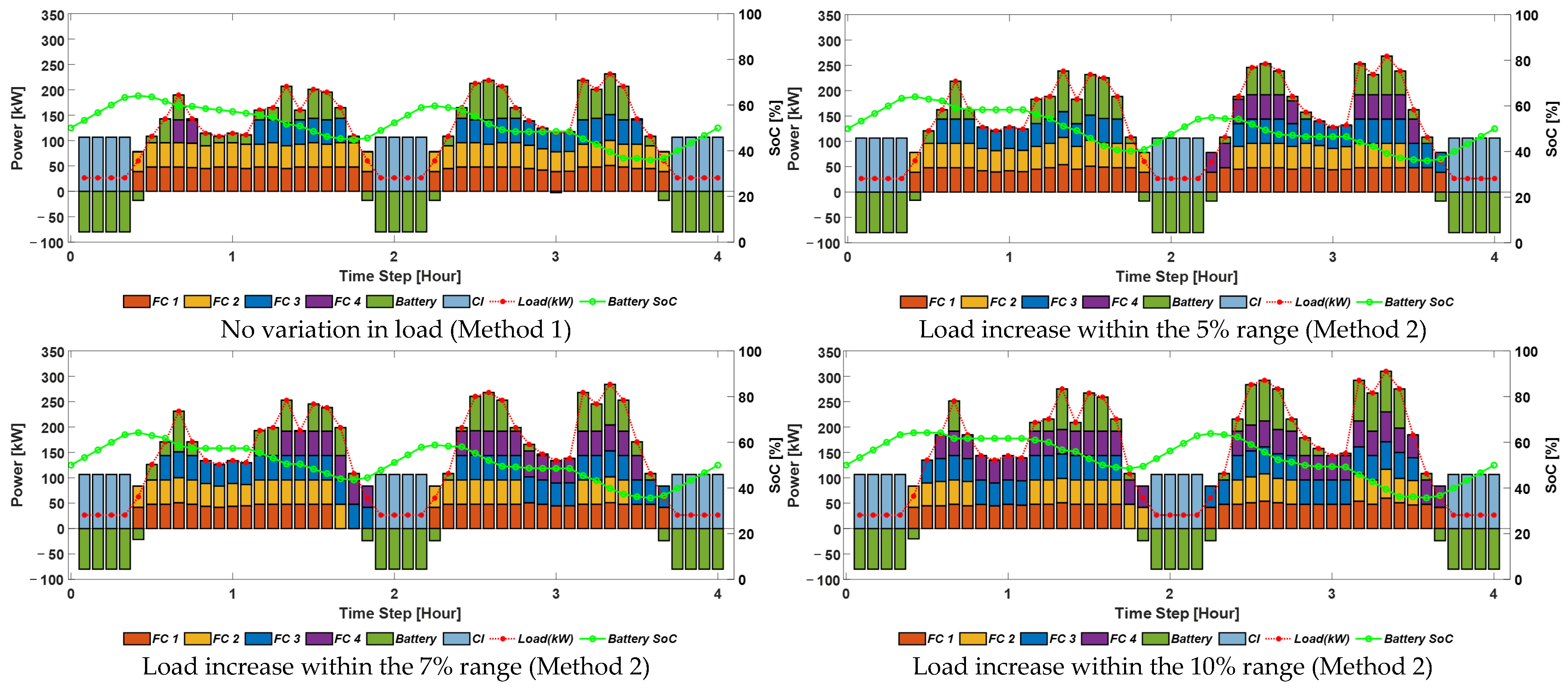
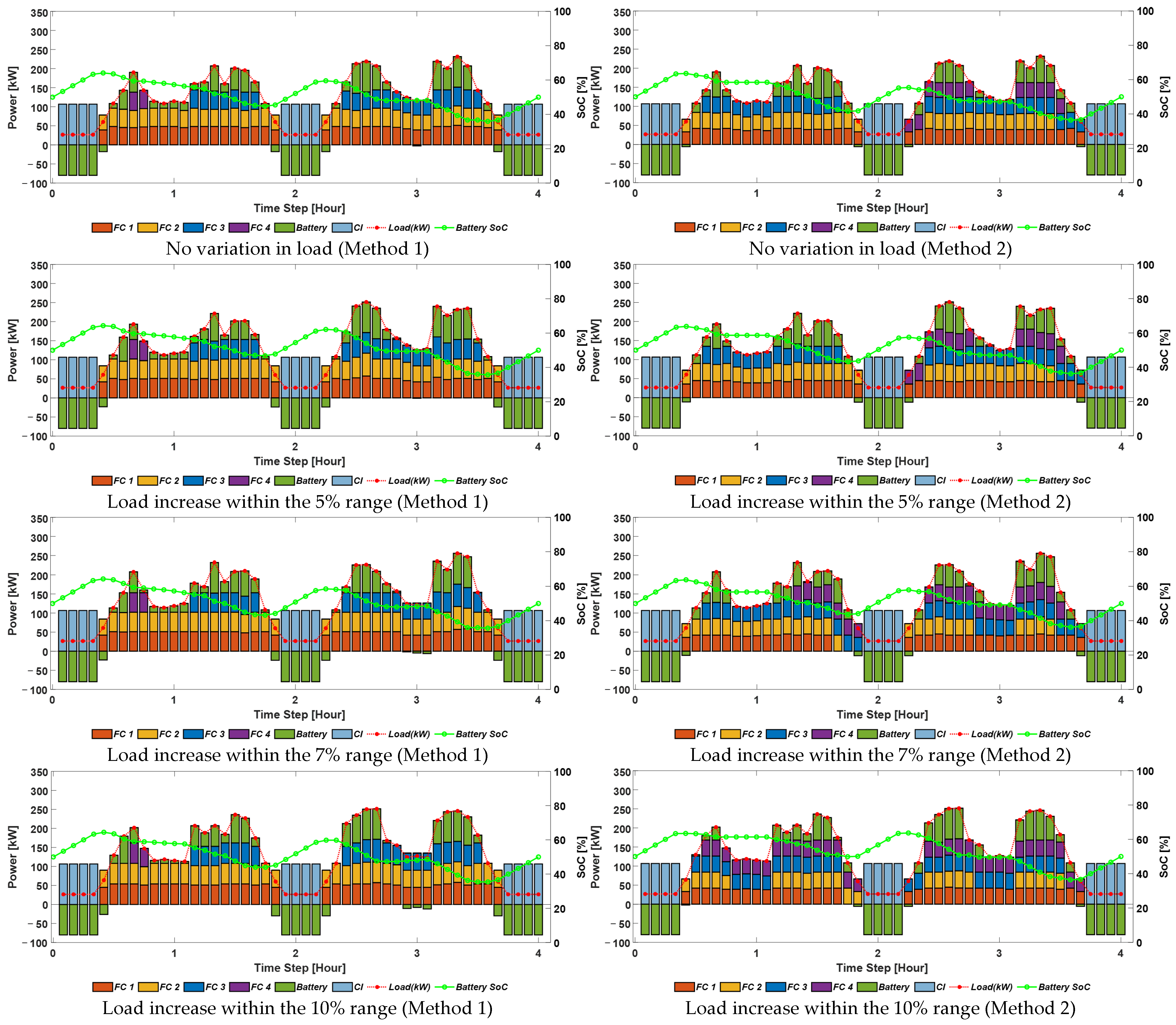
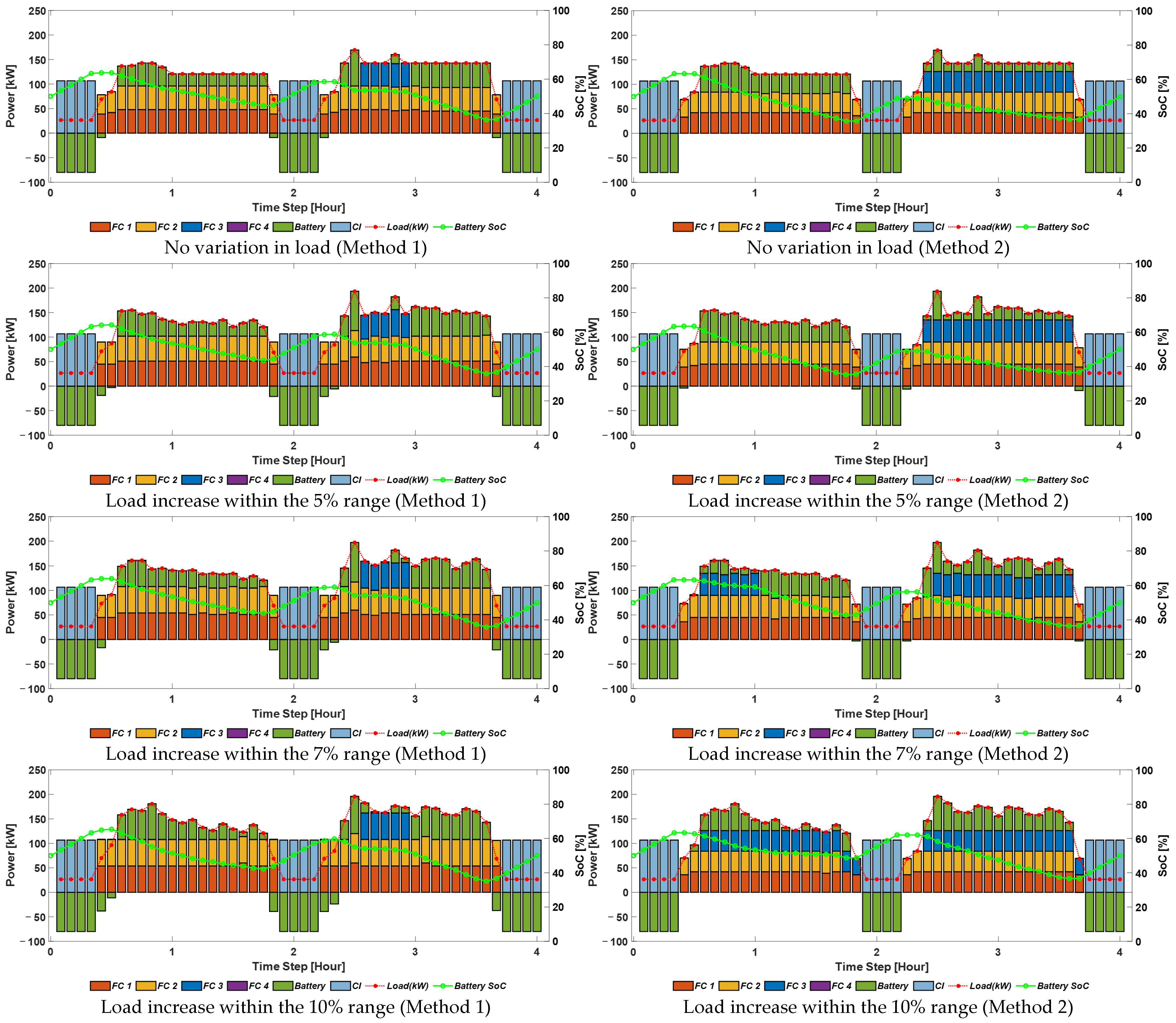
4.2. Optimal Power Generation Scheduling: Results and Analysis

This section evaluates the economic performance of two-stage scheduling methods based on MILP and robust optimization techniques through case studies. These methods involve a first-stage scheduling process for generator start-stop planning, followed by a second-stage scheduling for economic dispatch under realized uncertainties. The MILP-based method is referred to as Method 1, while the robust optimization-based method is referred to as Method 2.
In the first-stage pre-scheduling, Method 1 optimally dispatches generators based on the load profile, whereas Method 2 schedules for the worst-case scenario within the specified uncertainty range. The generator start–stop schedules determined in this stage are then applied to the second-stage real-time scheduling. Figure 9 presents the pre-scheduling results for both methods.
In the second-stage real-time scheduling, performance is analyzed based on the UC results obtained from pre-scheduling. Two scenarios are considered: one without load variation (where uncertainty is not realized) and another where load increases within uncertainty ranges of 5%, 7%, and 10%.
Figure 10 and Table 4 present the real-time scheduling results. For the no-load-variation case, real-time scheduling is based on the pre-scheduling result obtained from the 5% load increase scenario. When no uncertainty is realized, Method 1 provides the optimal solution for the given scenario, whereas Method 2 incurs a 1.35% increase in operational costs due to its conservative generator configuration, designed to handle uncertainty. This cost increase is primarily due to the higher degradation costs associated with operating multiple PEMFC units.
However, when the load increases within the 5%, 7%, and 10% uncertainty ranges, the total operational cost of Method 2 decreases. As the uncertainty range expands, the economic benefits of robust optimization become more pronounced. For instance, at 10% uncertainty, total operational costs are reduced by 7.69%, demonstrating that Method 2 offers superior fuel efficiency and cost-effectiveness under unexpected load increases. This is because in the first-stage pre-scheduling, load variations are considered, and a somewhat conservative generator operation plan is established. This strategy helps avoid high-output regions where efficiency drops significantly in the event of sudden load increases, contributing to reduced fuel consumption. Furthermore, by operating multiple PEMFC units in a distributed manner, the system is able to maintain operation within high-efficiency regions, resulting in reductions in both fuel and degradation costs. Additionally, hydrogen consumption is consistently lower in Method 2, regardless of whether uncertainty is realized.
Table 5 presents the results of a reliability analysis conducted by randomly generating 1500 scenarios with load variations within the 5%, 7%, and 10% uncertainty ranges. For Method 1, the proportion of infeasible scenarios increases significantly as uncertainty grows: 10.4% at 5% uncertainty, 33% at 7%, and 73.53% at 10%. This indicates a sharp decline in reliability under greater uncertainty. In contrast, Method 2 maintains full feasibility across all uncertainty levels, demonstrating its robustness against load variations.

4.3. Voyage Scheduling Analysis

This section integrates voyage scheduling into the optimal power generation scheduling process to achieve simultaneous optimization of both factors. In Method 1, power generation scheduling and voyage scheduling are conducted together in the first-stage scheduling. In contrast, Method 2 considers the worst-case scenario, using the optimal voyage schedule obtained in the first stage as a reference. The subsequent steps follow the same procedure as in Case Study 1. Figure 11 presents the first-stage pre-scheduling results.
In the second-stage real-time scheduling, the results are analyzed based on the UC information from the first stage, considering two cases: one without load variation, where uncertainty is not realized, and another where the load increases within the uncertainty range of 5%, 7%, and 10%.
Figure 12 and Table 6 present the real-time scheduling simulation results. The analysis of the no-load-variation case is based on the pre-scheduling result from the 5% load increase scenario.
When uncertainty is not realized, Method 1 provides the optimal solution, whereas Method 2 incurs a 1.01% increase in operational costs due to its conservative generator configuration designed for uncertainty. This cost increase is mainly attributed to the continued operation of multiple PEMFC units, which raises degradation costs.
In contrast, when the load increases within the 5%, 7%, and 10% uncertainty ranges, Method 2 demonstrates increasing economic benefits. At 10% uncertainty, total operational costs decrease by 6.13%. This indicates that robust optimization in Method 2 provides superior fuel efficiency and cost savings under unexpected load variations. Additionally, hydrogen consumption remains consistently lower in Method 2, regardless of whether uncertainty is realized.
Table 7 presents the reliability analysis results based on 1500 randomly generated scenarios under 5%, 7%, and 10% uncertainty levels, incorporating voyage scheduling. Compared to the results without voyage scheduling (Table 5), Method 1 shows a significant improvement in feasibility. At a 5% uncertainty level, all scenarios for Method 1 are feasible, indicating that voyage scheduling effectively ensures timely arrival and maintains power supply–demand balance under mild uncertainty.
However, at 7% uncertainty, 7.47% of scenarios become infeasible, and at 10%, this proportion increases to 20.47%, highlighting the limited robustness of Method 1 under severe conditions. In contrast, Method 2 maintains 100% feasibility across all uncertainty levels, confirming its superior ability to ensure operational stability even under worst-case conditions.

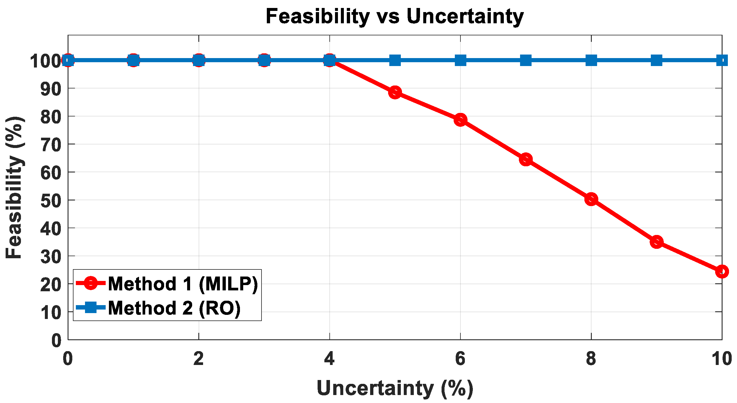
4.4. Sensitivity Analysis to Uncertainty

To quantify how increasing load uncertainty affects the total ship operational cost and feasibility in generation scheduling, we conducted a sensitivity analysis for uncertainty levels from 0% to 10% in 1% increments. At each level, we generated scenarios by randomly applying load increases or decreases within the specified uncertainty range, each scenario comprising 48 load values sampled at 5 min intervals over a 4 h period. We repeated scenario generation until 100 feasible solutions were obtained, and then calculated the total operational cost for both Method 1 (MILP) and Method 2 (robust optimization).
Figure 13 presents the cost distribution for each scenario, while the solid line shows the average cost at each uncertainty level. As uncertainty increases, Method 2 consistently achieves a lower average cost than Method 1, and the gap between the two widens. However, when uncertainty rises from 9% to 10%, a slight decrease in average cost appears due to sampling bias. At the 10% level, only 24.4% of generated scenarios were feasible, requiring 410 simulation runs to collect 100 feasible cases. Scenarios with high proportions of positive deviations across the 48 data points failed to satisfy system constraints and were discarded, leaving primarily scenarios dominated by negative deviations. Consequently, the average load of the selected scenarios was somewhat lower, reducing generator and ESS dispatch levels and biasing the average operational cost downward at the highest uncertainty level.
Figure 14 shows the operational feasibility rate, defined as the percentage of scenarios yielding a feasible solution at each uncertainty level. Method 1 achieves 100 percent feasibility for uncertainty levels up to 4%, but the feasibility rate drops significantly at 5% uncertainty and above, whereas Method 2 maintains 100% feasibility across all uncertainty levels. These results confirm that the robust optimization method reliably preserves system feasibility even as uncertainty increases.

5. Conclusions

The proposed robust optimization-based method for voyage and power generation scheduling enhances fuel efficiency and ensures a reliable power supply in PEMFC/BESS hybrid ships. Through case studies, this method was evaluated against the traditional MILP-based scheduling approach in terms of economic performance and reliability.
The MILP-based scheduling method delivers optimal results under predicted load conditions, maximizing efficiency when uncertainties are absent. However, in cases where load increases due to marine environmental variations, generator output may reach its limit, making operation infeasible. This limitation highlights the reduced reliability of the MILP-based method under uncertain conditions.
Conversely, the robust optimization-based approach incorporates marine environmental uncertainties, ensuring stable operation across various scenarios. By conservatively scheduling generator outputs, it enhances system robustness. This conservative strategy, however, results in additional generator usage, leading to higher PEMFC degradation costs and a slight increase in total operating expenses when uncertainties are not realized. Despite this drawback, when uncertainties do occur, the robust optimization method significantly improves economic efficiency and operational reliability.
For ships powered by conventional diesel or gas turbine generators, robust optimization leads to higher fuel costs than the MILP-based approach. However, in PEMFC-based ships, it reduces hydrogen consumption, as PEMFCs operate more efficiently at lower power outputs. The conservative generator scheduling in robust optimization enhances fuel efficiency, underscoring its advantages in hybrid ship applications.
In conclusion, this study compared the MILP-based and robust optimization-based scheduling methods, identifying their respective strengths and weaknesses. The findings confirm that robust optimization is a viable alternative for ensuring stability under uncertain conditions in PEMFC/BESS hybrid ships. Future research should focus on developing more advanced and practical optimization models that account for diverse environmental conditions and additional uncertainties, enabling power system scheduling methods that optimize both economic efficiency and operational reliability.

Author Contributions

Conceptualization, G.K. and I.-Y.C.; methodology, G.K.; software, G.K.; validation, G.K., M.L. and I.-Y.C.; formal analysis, G.K. and M.L.; investigation, G.K. and M.L.; data curation, M.L.; writing—original draft preparation, G.K.; writing—review and editing, G.K. and M.L.; visualization, M.L.; supervision, I.-Y.C.; project administration, I.-Y.C. All authors have read and agreed to the published version of the manuscript.

Funding

This work was supported by the Ministry of Science and ICT (MSIT), Korea through the NRF (National Research Foundation of Korea) under Grant RS-2024-00454464 and the ITRC (Information Technology Research Center) support program of the IITP (Institute for Information & Communications Technology Planning & Evaluation) under Grant RS-2023-00259004.

Data Availability Statement

The data presented in this study are available within the article.

Conflicts of Interest

The authors declare no conflicts of interest.

Nomenclature

Acronyms
BESSBattery energy storage system
CICold-ironing
C&CGColumn-and-constraint generation
DCDirect current
EDEconomic dispatch
ESSEnergy storage system
MILPMixed-integer linear programming
PEMFCPolymer electrolyte membrane fuel cell
SOCState of charge
UCUnit commitment
Variable and parameters
α h i g h Voltage drop per hour during high-power operation (μV/h)
α l o w Voltage drop per hour during low-power operation (μV/h)
α s t a r t Voltage drop per startup event (μV/start)
C B E S S , d e g t Degradation cost incurred by the BESS due to discharge at time t ($)
C F C , i t Fuel cost of the ith PEMFC at time t ($)
C F C , d e g , i t Degradation cost of the ith PEMFC at time t ($)
C H 2 Hydrogen cost (price) ($/kg)
C h i g h , i t Degradation cost due to high-power operation for the ith PEMFC at time t ($)
C i s o n , i t Degradation cost due to operating state for the ith PEMFC at time t ($)
C l o w , i t Degradation cost due to low-power operation for the ith PEMFC at time t ($)
C s t a r t u p , i t Degradation cost due to startup operations for the ith PEMFC at time t ($)
C C I t Cost of cold-ironing power at time t ($)
δ Speed uncertainty factor (dimensionless)
E B E S S Total energy capacity of the BESS (kWh)
E F C , i Energy output of the ith PEMFC (kWh)
H L H V Lower heating value of hydrogen (kWh/kg)
K E m Energy-to-hydrogen conversion factor (kg/kWh)
m H 2 Mass of hydrogen consumed (kg)
N F C Number of PEMFC units (dimensionless)
P B E S S , c h t BESS charge power at time t (kW)
P B E S S , d s c t BESS discharge power at time t (kW)
P C I t Cold-ironing power usage at time t (kW)
P F C , i t Output power of the ith PEMFC at time t (kW)
P L o a d t Total load demand at time t (kW)
P p r o p v Propulsion load as a function of ship speed v (kW)
p s t a c k Cost of the PEMFC stack ($)
S O C t State of charge of the BESS at time t (%)
S O C m i n Minimum allowable BESS state of charge (%)
S O C m a x Maximum allowable BESS state of charge (%)
S O C 0 Initial BESS state of charge at voyage start (%)
S O C f i n a l Final BESS state of charge at voyage end (%)
T E O L , F C Expected lifespan of the PEMFC (h)
T h i g h , i t High-power operation time for the ith PEMFC at time t (h)
T l o w , i t Low-power operation time for the ith PEMFC at time t (h)
U F C , i t Binary variable indicating whether the ith PEMFC is on at time t
U B E S S t Binary variable representing the charging/discharging state of the BESS
ξ F C t Binary variable indicating a startup event for the PEMFC at time t
η c h Charging efficiency of the BESS (%)
η d s c Discharge efficiency of the BESS (%)

Appendix A

Polynomial Fitting Evaluation

This appendix presents the quantitative evaluation results of the polynomial fittings performed for the PEMFC fuel cost function and the propulsion load curve data. All fittings were carried out using MATLAB’s polyfit and polyval functions. Fitting quality was assessed by Root Mean Square Error (RMSE) and coefficient of determination (R2). Optimal polynomial orders were chosen to balance model simplicity and avoid overfitting.
Table A1. Polynomial fitting results for PEMFC fuel cost function.
Polynomial OrderRMSE ($/h)R2
Linear (1st)1.25310.9843
Quadratic (2nd)0.14990.9997
Cubic (3rd)0.14990.9997
Quartic (4th)0.14730.9997
For the PEMFC fuel cost function, the quadratic fit was selected as most suitable. Although the quartic model marginally reduced RMSE, it introduced unnecessary complexity and risked overfitting.
Table A2. Polynomial fitting results for propulsion load curve.
Polynomial OrderRMSE (kW)R2
Linear (1st)27.4460.9376
Quadratic (2nd)1.23250.9999
Cubic (3rd)6.33 × 10−141.0000
For the propulsion load curve, the cubic fit perfectly interpolated the four data points, delivering the highest accuracy without over-parameterization. Higher-order fits were not evaluated due to the limited number of points.
These results justify the chosen polynomial approximations in the main text and clarify the criteria used to select the final models.

References

  1. International Maritime Organization. 2023 IMO Strategy on Reduction of GHG Emissions from Ships (MEPC 80/WP.12, Annex 1); International Maritime Organization: London, UK, 2023. [Google Scholar]
  2. Korea Maritime Cooperation Center. International Trend for Maritime Decarbonization; Korea Maritime Cooperation Center: Sejong-si, Republic of Korea, 2023; Volume 7. [Google Scholar]
  3. Kim, S.N.; Park, Y.H. DC Electric propulsion ship technology trend. Korean Inst. Electr. Eng. 2018, 67, 25–31. [Google Scholar]
  4. Jeong, D.W. Optimal Operation Strategy for Power Generation System of Electric Propulsion Ships Based on Lagrangian Relaxation Method for Fuel Cost Reduction. Master’s Thesis, Kookmin University, Seoul, Republic of Korea, 2022. [Google Scholar]
  5. Lee, J.M.; Kim, J.H.; Kim, S.G.; Kim, T.W.; Kim, M.S. Overview and technology development trends of hydrogen fuel cell ships. Bull. Soc. Nav. Archit. Korea 2019, 56, 3–9. [Google Scholar]
  6. Seo, Y.S.; Cho, J.H.; Lee, J.M.; Kim, B.S. Development Trends and Directions of Hydrogen Fuel Cell Technology for Ships; KEIT PD Issue Report; Korea Institute for Advancement of Technology: Seoul, Republic of Korea, 2019. [Google Scholar]
  7. Chandran, M.; Palaniswamy, K.; Karthik Babu, N.B.; Das, O. A study of the influence of current ramp rate on the performance of polymer electrolyte membrane fuel cell. Sci. Rep. 2022, 12, 21888. [Google Scholar] [CrossRef] [PubMed]
  8. Pivetta, D.; Dall’Armi, C.; Taccani, R. Multi-objective optimization of hybrid PEMFC/Li-ion battery propulsion systems for small and medium size ferries. Int. J. Hydrogen Energy 2021, 46, 35949–35960. [Google Scholar] [CrossRef]
  9. Switch Maritime. Available online: https://www.switchmaritime.com/ (accessed on 1 January 2025).
  10. Choi, C.H.; Yu, S.; Han, I.S.; Kho, B.K.; Kang, D.G.; Lee, H.Y.; Seo, M.S.; Kong, J.W.; Kim, G.; Ahn, J.W.; et al. Development and demonstration of PEM fuel-cell-battery hybrid system for propulsion of tourist boat. Int. J. Hydrogen Energy 2016, 41, 3591–3599. [Google Scholar] [CrossRef]
  11. Kanellos, F.D.; Anvari-Moghaddam, A.; Guerrero, J.M. A cost-effective and emission-aware power management system for ships with integrated full Electric propulsion. Electr. Power Syst. Res. 2017, 150, 63–75. [Google Scholar] [CrossRef]
  12. Aziz, M.; Trinh, P.-H.; Hudaya, C.; Chung, I.-Y. Coordinated control strategy for hybrid multi-PEMFC/BESS in a shipboard power system. Electr. Power Syst. Res. 2025, 243, 111495. [Google Scholar] [CrossRef]
  13. Fang, S.; Xu, Y.; Li, Z.; Zhao, T.; Wang, H. Two-step multi-objective management of hybrid energy storage system in all-Electric ship microgrids. IEEE Trans. Veh. Technol. 2019, 68, 3361–3373. [Google Scholar] [CrossRef]
  14. Taheri, S.I.; Vieira, G.G.T.; Salles, M.B.C.; Avila, S.L. A trip-ahead strategy for optimal energy dispatch in ship power systems. Electr. Power Syst. Res. 2021, 192, 106917. [Google Scholar] [CrossRef]
  15. Shapiro, A. Topics in Stochastic Programming; CORE Lecture Series; Universite Catholique de Louvain: Ottignies-Louvain-la-Neuve, Belgium, 2011. [Google Scholar]
  16. Jin, Y.; Wang, H.; Chugh, T.; Guo, D.; Miettinen, K. Data-Driven Evolutionary Optimization: An Overview and Case Studies. IEEE Trans. Evol. Comput. 2019, 23, 442–458. [Google Scholar] [CrossRef]
  17. Ksciuk, J.; Kuhlemann, S.; Tierney, K.; Koberstein, A. Uncertainty in maritime ship routing and scheduling: A literature review. Eur. J. Oper. Res. 2023, 308, 499–524. [Google Scholar] [CrossRef]
  18. Fang, S.; Xu, Y.; Wang, H.; Shang, C.; Feng, X. Robust operation of shipboard microgrids with multiple-battery energy storage system under navigation uncertainties. IEEE Trans. Veh. Technol. 2020, 69, 10531–10544. [Google Scholar] [CrossRef]
  19. Li, Z.; Xu, Y.; Fang, S.; Zheng, X.; Feng, X. Robust coordination of a hybrid AC/DC multi-energy ship microgrid with flexible voyage and thermal loads. IEEE Trans. Smart Grid 2020, 11, 2782–2793. [Google Scholar] [CrossRef]
  20. Kim, G.B.; Aziz, M.; Trinh, P.H.; Chung, I.Y. Optimal design and scheduling methods for fuel cell and battery energy storage systems in Electric ships. In Proceedings of the ICEE Conference, Kitakyushu, Japan, 30 June–4 July 2024. [Google Scholar]
  21. Sery, J.; Leduc, P. Fuel cell behavior and energy balance on board a Hyundai Nexø. Int. J. Engine Res. 2022, 23, 709–720. [Google Scholar] [CrossRef]
  22. Banaei, M.; Rafiei, M. A comparative analysis of optimal operation scenarios in hybrid emission-free ferry ships. IEEE Trans. Transp. Electrif. 2020, 6, 318–333. [Google Scholar] [CrossRef]
  23. Jeong, B.H. Generator Scheduling Methods for Fuel Cost Reduction in Electrical Shipboard Power Systems Using Load Forecasting. Master’s Thesis, Kookmin University, Seoul, Republic of Korea, 2023. [Google Scholar]
  24. Angkasa, F.F. Optimal Power Generation and Voyage Scheduling with Operating Reserve Management for Electric Ship. Master’s Thesis, Kookmin University, Seoul, Republic of Korea, 2022. [Google Scholar]
  25. Fan, F.; Aditya, V.; Xu, Y.; Cheong, B.; Gupta, A.K. Robustly coordinated operation of a ship microgrid with hybrid propulsion systems and hydrogen fuel cells. Appl. Energy 2022, 312, 118738. [Google Scholar] [CrossRef]
  26. Bialystocki, N.; Konovessis, D. On the estimation of ship’s fuel consumption and speed curve: A statistical approach. J. Ocean Eng. Sci. 2016, 1, 157–166. [Google Scholar] [CrossRef]
  27. Zhao, L.; Zeng, B. An Exact Algorithm for Two-Stage Robust Optimization with Mixed Integer Recourse Problems. 2012. Available online: https://optimization-online.org/2012/ (accessed on 1 January 2025).
  28. Zeng, B.; Zhao, L. Solving two-stage robust optimization problems using a column-and-constraint generation method. Oper. Res. Lett. 2013, 41, 457–461. [Google Scholar] [CrossRef]
  29. Liu, R.S.; Hsu, Y.F. A scalable and robust approach to demand side management for smart grids with uncertain renewable power generation and bi-directional energy trading. Int. J. Electr. Power Energy Syst. 2018, 97, 396–407. [Google Scholar] [CrossRef]
  30. Li, M.; Liu, H.; Yan, M.; Xu, H.; He, H. A novel multi-objective energy management strategy for fuel cell buses quantifying fuel cell degradation as operating cost. Sustainability 2022, 14, 16190. [Google Scholar] [CrossRef]
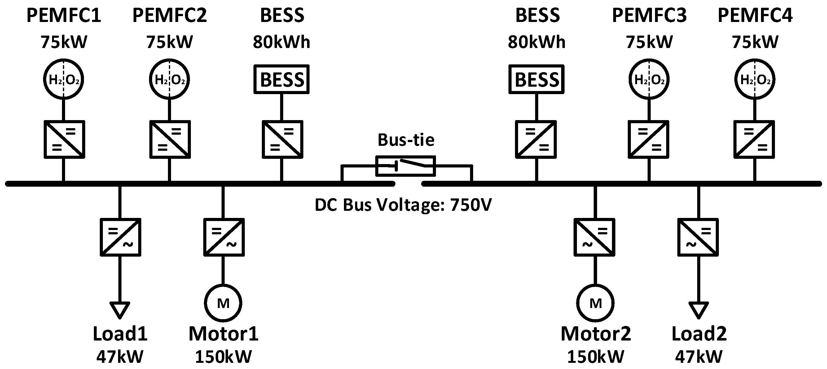
Figure 1. Configuration of the PEMFC/BESS hybrid ship.
Energies 18 02837 g001
Figure 2. Fuel efficiency and cost of the PEMFC (75 kW rated). (a) PEMFC efficiency and hydrogen consumption curves; (b) PEMFC fuel cost function.
Energies 18 02837 g002
Figure 3. Propulsion load curve corresponding to the ship’s speed.
Energies 18 02837 g003
Figure 4. Two-stage power generation scheduling with robust coordination strategy.
Energies 18 02837 g004
Figure 5. Example of load uncertainty range due to speed loss (10% variation).
Energies 18 02837 g005
Figure 6. Flowchart of the robust optimal power scheduling with the C&CG methodology.
Energies 18 02837 g006
Figure 7. Configuration of the integrated power system for the target ship.
Energies 18 02837 g007
Figure 8. Load profile.
Energies 18 02837 g008
Figure 9. Optimal pre-scheduling results.
Energies 18 02837 g009
Figure 10. Optimal power generation scheduling results (5%, 7%, and 10% load variations).
Energies 18 02837 g010
Figure 11. Optimal pre-scheduling results with voyage scheduling.
Energies 18 02837 g011
Figure 12. Optimal voyage and power generation scheduling results (5%, 7%, and 10% load variations).
Energies 18 02837 g012
Figure 13. The total operational cost under different uncertainty levels for MILP and robust optimization.
Energies 18 02837 g013
Figure 14. Feasibility rate under uncertainty for MILP and robust optimization.
Energies 18 02837 g014
Table 1. Rated capacity of the integrated power system.
ComponentsCapacity
PEMFC75 kW
BESS80 kWh
Propulsion Motor150 kW
Main Bus750 V
Table 2. Output range of the power generation system.
PEMFC Output and Operating Range
TypeRated Capacity (kW)Minimum Output (kW)Maximum Output (kW)
PEMFC757.567.5
BESS Output and Operating Range
TypeRated Capacity (kWh)Min, Max SOC (%)C-rateConverter Efficiency (%)
BESS8010, 900.595
Table 3. Parameters for the case study.
PEMFC Cost Function
a i b i c i
0.0010190.99596.244
Propulsion motor
c 3 c 2 c 1 c 0
0.3274−2.5857.4260.0131
Parameters
Hydrogen Cost ($)7 C B E S S , d e g ($/kWh)0.38
K E m (kg/kWh)0.03 C e l e c t r i c   c h a r g e ($/kWh)0.01
α h i g h ,     α l o w ,     α s t a r t (μV)10, 8.662, 23.91 u E o L , F C (μV)6000
p s t a c k ($)28,000 T E o L , F C (h)5000
m 1 ,   m 2 , s t a r t ,   m 3 ,   m 4 1 m 2 , h i g h ,   m 2 , i s o n ,   m 2 ,   l o w ,10
Table 4. Comparison of optimal power generation scheduling results (5%, 7%, and 10% load variations).
No Variation in LoadLoad Increase Within the 5% RangeLoad Increase Within the 7% RangeLoad Increase Within the 10% Range
MethodMethod 1Method 2Method 1Method 2Method 1Method 2Method 1Method 2
H2 consumption Cost ($)121.98118.90133.65129.82134.73129.87142.02134.98
FC degradation Cost ($)37.7143.2744.2043.2750.6844.9357.1648.16
BESS degradation cost ($)2.732.602.792.662.822.662.922.59
Cold-ironing cost ($)10.6610.6610.6610.6610.6610.6610.6610.66
Total cost ($)173.09175.43191.29186.40198.88188.13212.76196.39
Total cost change ($)-2.34
(+1.35%)
-−3.27
(−1.89%)
-−10.76
(−5.41%)
-−16.37
(−7.69%)
H2 cost change ($)-−3.08
(−2.53%)
-−3.81
(−3.13%)
-−4.85
(−3.60%)
-−7.03
(−4.95%)
Table 5. Results of reliability analysis of optimal power generation scheduling.
Uncertainty Range5%7%10%
MethodMethod 1Method 2Method 1Method 2Method 1Method 2
Feasible scenarios13441500100515003971500
Infeasible scenarios156 (10.4%)0495 (33%)01103 (73.53%)0
Table 6. Comparison of optimal voyage and power generation scheduling results (5%, 7%, and 10% load variations).
No Variation in LoadLoad Increase Within the 5% RangeLoad Increase Within the 7% RangeLoad Increase Within the 10% Range
MethodMethod 1Method 2Method 1Method 2Method 1Method 2Method 1Method 2
H2 consumption Cost ($)100.3698.02109.90107.03115.00110.58121.76114.81
FC degradation Cost ($)30.4934.3833.7434.3836.9836.4443.4639.94
BESS degradation cost ($)2.632.532.772.602.762.563.032.53
Cold-ironing cost ($)10.6610.6610.6610.6610.6610.6610.6610.66
Total cost ($)144.14145.59157.07154.67165.39160.24178.91167.95
Total cost change ($)-1.45
(+1.01%)
-−2.40
(−1.53%)
-−5.16
(−3.12%)
-−10.96
(−6.13%)
H2 cost change ($)-−2.34
(−2.33%)
-−2.87
(−2.61%)
-−4.42
(−3.84%)
-−6.94
(−5.70%)
Table 7. Results of reliability analysis of optimal voyage and power generation scheduling.
Uncertainty Range5%7%10%
MethodMethod 1Method 2Method 1Method 2Method 1Method 2
Feasible scenarios150015001388150011931500
Infeasible scenarios0 (0%)0112 (7.47%)0307 (20.47%)0
Disclaimer/Publisher’s Note: The statements, opinions and data contained in all publications are solely those of the individual author(s) and contributor(s) and not of MDPI and/or the editor(s). MDPI and/or the editor(s) disclaim responsibility for any injury to people or property resulting from any ideas, methods, instructions or products referred to in the content.

