Enhanced Oil Production Forecasting in CCUS-EOR Systems via KAN-LSTM Neural Network

Abstract

The accurate forecasting of crude oil production in CCUS-EOR (carbon capture, utilization, and storage–enhanced oil recovery) operations is essential for the economic evaluation and production optimization of oilfield blocks. Although numerous deep learning models have been widely applied for this purpose, existing methods still face challenges in extracting complex features from multidimensional time series datasets, limiting the accuracy of oil production forecasts. In this study, we propose a novel KAN-LSTM model that integrates a KAN (knowledge-aware network) layer with a long short-term memory (LSTM) neural network to enhance the accuracy of oil production forecasting in CCUS-EOR applications. The KAN layer effectively extracts relevant features from multivariate data, while the LSTM layer models temporal information based on the extracted features to generate accurate predictions. To evaluate the performance of the proposed model, we conducted two case studies using both mechanistic model data and real project production data. The prediction performance of our method was compared with that of typical deep learning approaches. Experimental results demonstrate that the KAN-LSTM model outperforms other forecasting methods. By providing reliable estimates of future oil production, the KAN-LSTM model enables engineers to make informed decisions in reservoir development planning.

1. Introduction

In the petroleum industry, achieving rapid, reliable, and cost-effective predictions is a crucial task. It can significantly enhance the efficiency of future development planning and boost recovery rates [1]. Daily production generates vast amounts of data. However, these data are often constrained by regional economic conditions and production costs (such as CO₂ pricing), which impede the timely intelligent upgrading of production equipment. Production dynamics are largely reliant on manual statistics, frequently leading to production halts or data gaps. These issues compromise the accuracy of the data and make it challenging for managers to access sufficient and reliable information to accurately predict production dynamics.

To address these requirements, mechanism-based and data-driven prediction methods have emerged as mainstream research directions. Most mechanism-based methods, such as reservoir numerical simulation [2,3], typically employ a bottom-up modeling approach to construct models. Establishing a model to simulate reservoir behavior requires obtaining extensive underground data. This process demands a significant amount of data and can take hours to approximate a solution. It also has high data quality requirements, making it difficult to detect occasional data recording errors. Moreover, it struggles to quickly adapt to sudden changes in production dynamics, such as weekly shutdowns.

In numerical simulation, the reservoir is discretized into a grid, necessitating comprehensive data collection for accurate simulation. However, subtle changes in the formation during production may occur, requiring meticulous and expensive formation testing [4]. This is particularly problematic for cost-sensitive oil reservoirs that are already in production, as the process then becomes economically unfeasible.

Over the past few decades, various mechanism-based methods have been developed for production prediction. Early approaches typically employed simple statistical methods to analyze and organize the relationships between dynamic indicators generated in oil fields (such as blocks or individual wells), thereby deriving corresponding mathematical models. These methods gained widespread use in practical applications—such as A-, B-, C-, and D-type water–drive characteristic curves [5,6]—due to their convenient and accurate data sources, straightforward relationships between relevant indicators, and simple data processing procedures. However, because of their fixed model types, it is essential to assess the applicability of these characteristic curves during use. Significant deviations may occur if there are changes in injection and production methods or injection materials.

With the advancement of deep learning, this method has outperformed traditional ones by automatically extracting temporal and robust features from training data. As a result, deep learning has achieved remarkable success in the field of time series prediction [7,8,9,10]. Currently, numerous classical deep learning methods have been successfully applied to the time series prediction of reservoir production, yielding promising results. For instance, various architectures based on multilayer perceptron (MLP), such as fully connected neural networks (FCNNs), recurrent neural networks (RNNs), and long short-term memory networks (LSTM), have been developed. These models effectively capture both the temporal dynamics of time series data and the complex underlying geological patterns [11,12,13,14,15]. Among them, LSTMs have emerged as the most widely used tools for characterizing reservoir production. By leveraging deep learning-based time series network models, they overcome the limitations of traditional statistical models and address the inherent complexities of reservoir engineering predictions [4]. However, these models also face several challenges during the training process. They are susceptible to issues such as gradient vanishing and exploding, which can impede the learning process and increase training time. Moreover, their ability to capture the intrinsic relationships within multidimensional data needs to be further enhanced. Additionally, they often struggle to provide accurate and sustained long-term predictions, and they all face challenges in adapting to continuous learning scenarios. To solve these problems, hybrid models combining different types of neural networks or machine learning models have also received widespread attention in recent years to improve prediction accuracy [16,17,18,19]. They have good accuracy, but their training speed is relatively slow, and it is hard to combine geological information itself. To address the aforementioned issues, Liu et al. [20] proposed the Kolmogorov–Arnold network (KAN) [21] to fit mathematical and natural science problems. An increasing number of studies [22,23,24] demonstrate that the KAN excels in fitting special functions in mathematics and physics. When the number of parameters is the same, the KAN can achieve lower training and testing losses compared to MLP. The KAN also shows strong capabilities in fitting high-dimensional functions. Moreover, the KAN can represent the learned physical models in the form of symbolic formulas, making the physical meanings of the models more intuitive and understandable. The KAN allows users to strike a balance between simplicity and accuracy. By adding more inductive biases or manually setting the forms of certain activation functions, one can obtain simpler or more accurate symbolic formulas, thereby better adapting to different physical problems. In terms of continual learning, the KAN, leveraging the locality of spline functions, can retain learned information and adapt to new data without catastrophic forgetting, giving it an edge in dealing with dynamically changing physical systems.

In this study, the KAN is employed to replace the conventional multilayer perceptron (MLP), and a deep learning model named KAN-LSTM is proposed. For the first time, this model is introduced to the field of oil prediction. This substitution significantly enhances the model’s ability to perceive time series and geological fuzzy information. Moreover, it enables the model to automatically and rapidly learn injection and production patterns without requiring additional inputs. In addition, we compared the predictive performance and speed of the KAN-LSTM model on the CCUS-EOR dataset with two other hybrid KAN models, namely TCN-KAN and GRU-KAN [25]. The results show that KAN-LSTM exhibits slightly superior predictive ability on the CCUS-EOR data compared to GRU-KAN and TCN-KAN. Moreover, KAN-LSTM achieves this enhanced performance with faster training and testing speeds than the other two hybrid KAN models.

2. Methodologies

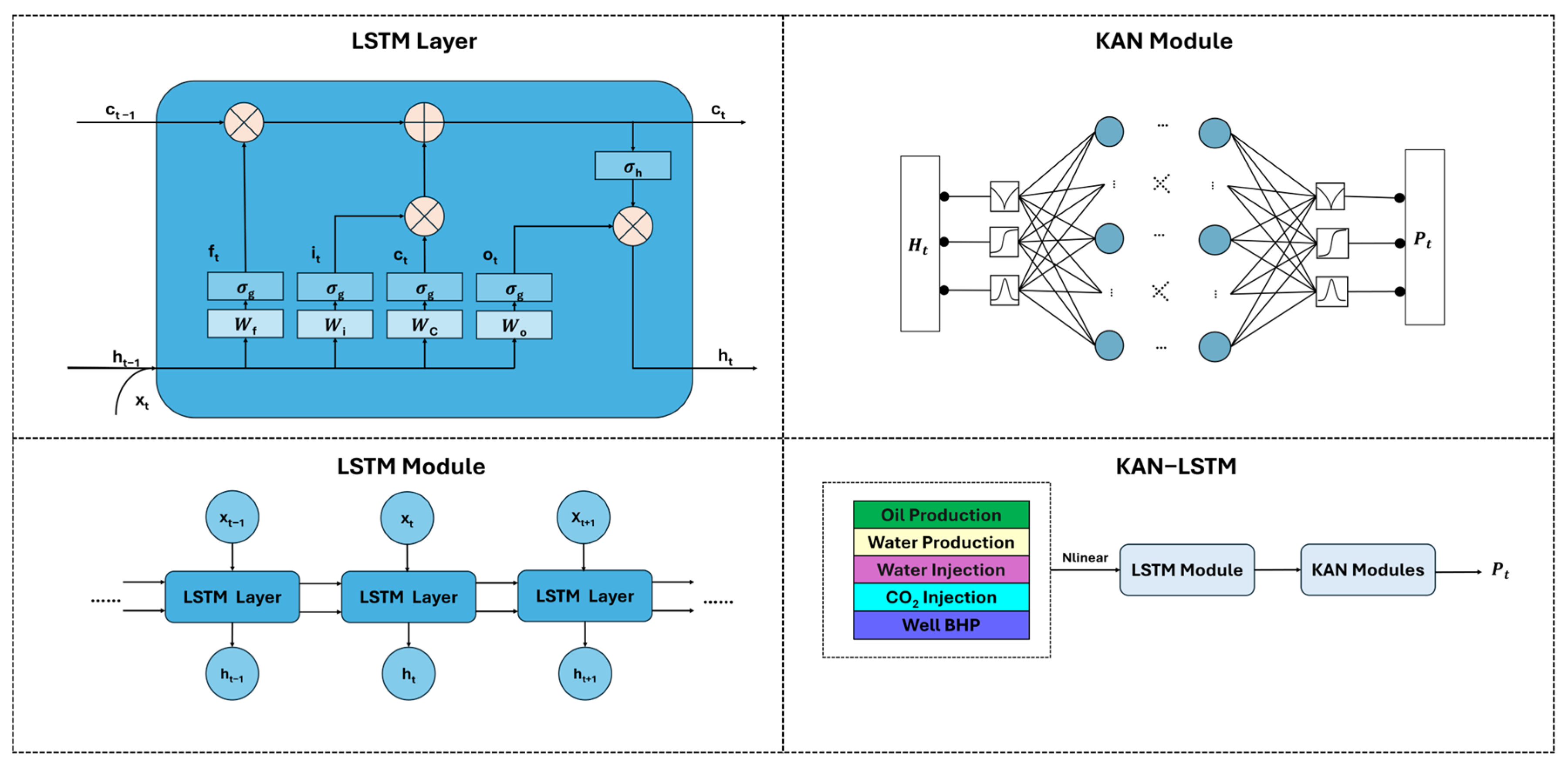
The overall architecture of the proposed KAN-LSTM is shown in Figure 1. Initially, the input variables undergo the NLinear operation, which performs linear filtering and blends temporal data features. Subsequently, these variables are mapped into a time series network module and then transmitted to the subsequent KAN. The construction and optimization of the model are detailed in the subsequent sections.

2.1. Model Predicting Workflow

The overall architecture of the proposed KAN-LSTM is illustrated in Figure 1. Initially, the input variables (production, injection, pressure, average porosity, etc.) are processed through NLinear modules, which perform linear filtering and blend temporal data features. Subsequently, these variables are mapped into a time series network module and then transmitted to the subsequent KAN. The construction and optimization of the model are detailed in the next sections.

The oil production forecasting issue is formulated as a time series prediction problem. The production at each time point $t$ is denoted by $p_{t_0}^1$, $p_{t_0}^2$…$p_{t_0}^k$. Among them, k represents the number of parameters, and its feature matrix is represented by $Y_{t_0}$. The assignment of the task is to predict the future values of the series

$$Y=\left[Y_{t_0},\cdots ,Y_{t_0+T}\right]=\left[\begin{array}{l}{P}^1\\ ⋮\\ P^k\end{array}\right]=\left[\begin{array}{l}{p}_{t_0}^1,p_{t_0+1}^1,\cdots ,p_{t_0+T}^1\\ ⋮\\ p_{t_0}^k,p_{t_0+1}^k,\cdots ,p_{t_0+T}^k\end{array}\right]$$

based on its historical values and feature matrix

$$Y=\left[Y_1,Y_2,\cdots ,Y_{t_0-1}\right]$$

where $t$ denotes the starting point from which future data $p_t^1$, $t=t_0\dots t_0+T$ are to be predicted. The model distinguishes between the historical period, denoted as $[1,t_0-1]$, which represents the context length, and the forecast period, denoted as $[t_0,t_0+T]$, which represents the prediction length.

2.2. KAN-LSTM Model

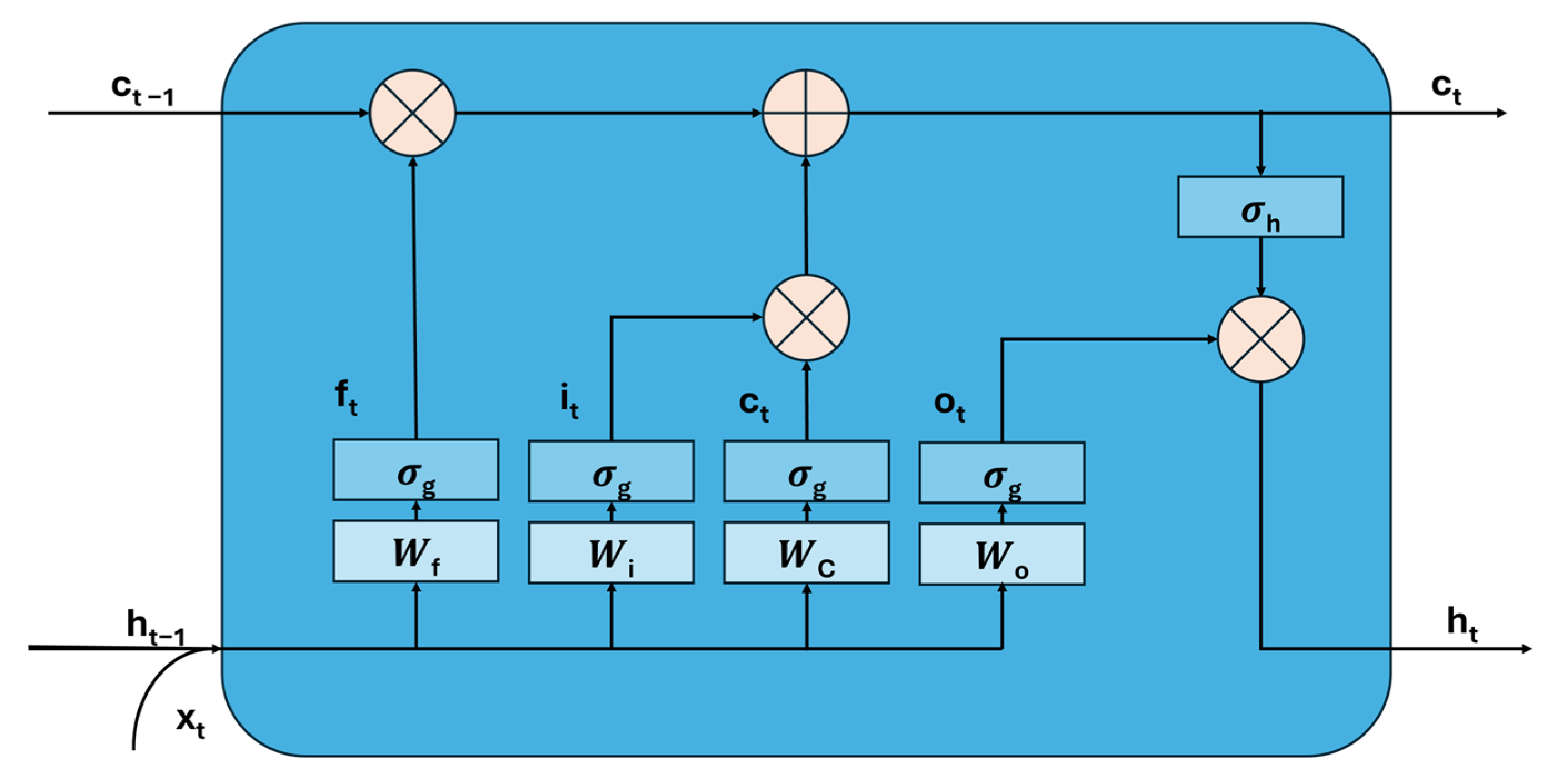
2.2.1. LSTM Module

LSTM (long short-term memory network) is a popular recurrent neural network (RNN) architecture that includes feedback connections. This unique structure makes LSTM perform well in processing time series data. Compared to other RNN-based variants such as bidirectional LSTM and BiLSTM, traditional LSTM is more concise and efficient in terms of computational complexity [26]. Lindemann et al.’s research [27] also indicates that LSTM networks have significant advantages in detecting anomalies and learning temporal relationships in time-dependent backgrounds. A standard LSTM unit consists of an input gate ($i$), a forget gate ($f$), and an output gate ($o$) [28], as shown in Figure 2. The LSTM unit dynamically adjusts the required estimation parameters based on the model input through input gates, forget gates, and output gates.

2.2.2. Kolmogorov–Arnold Network (KAN) Module

The Kolmogorov–Arnold representation theorem is a cornerstone of dynamic systems theory and traversal theory, independently proposed by Andrei Kolmogorov and Vladimir Arnold in the mid-20th century [21]. This theorem states that within a finite interval, any multivariate continuous function $f$, dependent on the variable $x=[x_1,x_2,\cdots ,x_n]$, can be represented by a finite combination of simpler continuous functions involving only a single variable. Specifically, a real valued, smooth, and continuous multivariate function $f(x)$ defined on $[0,1]$ can be approximated by the superposition of a finite number of univariate functions, as shown in Equation(1):

$$f(x)={\displaystyle \sum _{i=1}^{2n+1}{\mathsf{\Phi }}_i\left({\displaystyle \sum _{j=1}^n{\varphi }_{i,j}(x_j)}\right)}$$

(1)

where ${\mathsf{\Phi }}_i$ and ${\varphi }_{i,j}$ represent the external and internal real functions, respectively.

In a multi-layer perceptron (MLP) [29], the learning process involves optimizing the weights, while the activation functions on each node remain fixed. In contrast, the KAN (Kolmogorov–Arnold network) learns the activation function of each node individually. Instead of linear weights, the KAN employs univariate spliced functions. When a neural network aims to learn a high-precision function, it must approximate both the univariate functions and the compositional structure of the problem. The KAN, proposed by Liu et al. [21], integrates splines with the MLP architecture to achieve a high degree of robustness, accuracy, and adaptability.

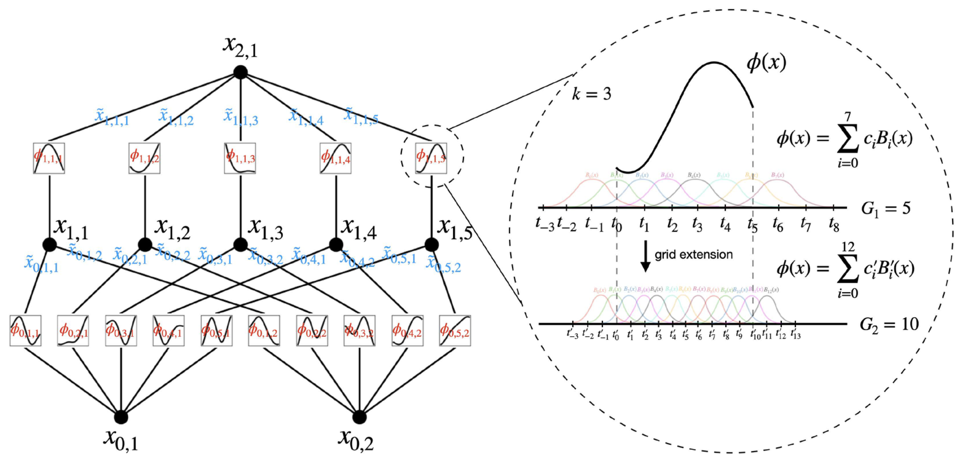
The multivariate function $f(x)$ has two layers of nonlinearity, with 2n + 1 terms (n is the number of input variables) in the middle layer. Therefore, a suitable function in the univariate function only needs to be found, that is, a univariate function (${\varphi }_{i,j}$, and ${\mathsf{\Phi }}_i$) that approximates the function. The one-dimensional functions ${\varphi }_{i,j}$ can be approximated by B-splines [30]. When using the spline, it should be characterized by its order $k$—commonly set to 3 for cubic splines—determines the degree of the polynomials that define the curve segments between control points. The intervals, represented by $G$, signify the count of segments dividing the space between each pair of consecutive control points. During spline interpolation, these segments seamlessly link the data points, creating a smooth curve that comprises $G+1$ grid points. B-spline functions [31] are employed because of their exceptional stability and accuracy in numerical computations. They are particularly effective for approximating low-dimensional functions and enable transformations across various resolutions, making them an ideal choice for approximation tasks. Additionally, wider and deeper KANs have been proposed for deep learning applications to capture more complex nonlinear features.

In the Kolmogorov–Arnold network (KAN), each KAN layer is defined by a matrix $\mathsf{\Phi }$ consisting of a series of univariate functions $\left\{{\varphi }_{i,j}\left(.\right)\right\}$. The range of $i$ here is from 1 to n, representing the number of input variables, while the range of j is from 1 to N, representing the number of output variables. Each ${\varphi }_{i,j}$ is a trainable spline function, as mentioned earlier.

The architecture of a KAN layer can be characterized with the notation $[n_1,\cdots ,n_{L+1}]$, where $L$ represents the total number of layers within the KAN. It is important to note that the Kolmogorov–Arnold theorem corresponds to a specific KAN configuration with the structure $[n,2n+1,1]$. A more complex, multi-layered KAN can be represented as Equation (2), with $L$ layers:

$$\mathrm{y}=\mathrm{KAN}\left(\mathrm{x}\right)=({\mathsf{\Phi }}_L\circ {\mathsf{\Phi }}_{L-1}\circ \cdots \circ {\mathsf{\Phi }}_1)•\mathrm{x}$$

(2)

This is because all of its operations are differentiable. So, the KAN can be trained through backpropagation. As the KAN has an elegant mathematical foundation, it effectively utilizes the advantages of B-spline functions and MLP on the basis of simple modifications to MLP while mitigating their respective weaknesses. Each connection in the network is equipped with weight parameters and trainable activation functions, giving the network the ability to automatically find the best nonlinear transformation. This design greatly enhances the flexibility in handling nonlinear problems, especially suitable for scenarios with complex data distributions or highly nonlinear relationships. Enhancing the number of layers $L$ in a KAN or the dimensionality of the grid $G$ effectively increases the quantity of parameters and the complexity of the network. The structure of the KAN module is illustrated in Figure 3.

This method provides a new optimization solution for traditional deep learning (DL) models that mainly utilize the multilayer perceptron (MLP) architecture for prediction and provides us with a way to further explore and expand new methods for time series analysis.

3. Case Studies

The performance of the proposed KAN-LSTM model is evaluated using both reservoir numerical simulation data and real-world reservoir operation data. We compare our method with three state-of-the-art production prediction techniques, namely the temporal convolutional network (TCN), long short-term memory (LSTM), gated recurrent units (GRUs), and two hybrid models, namely GRU-KAN and TCN-KAN. The baseline methods are implemented with the hyperparameters recommended in their original papers.

Three evaluation indicators are employed, including the mean square error (MSE), root mean square error (RMSE), and the coefficient of determination (R²) [9]; these indicators are employed to assess the model’s performance across training, testing, and validation datasets. Such evaluations are crucial for diagnosing potential overfitting or underfitting issues within the model’s interaction with the dataset.

A. Configuration for Hyperparameters

The KAN-LSTM model is constructed by integrating the time series network with the KAN model. The specific configurations, including the number of layers and the grid dimensionality of the KANs, as well as other relevant model parameters, are detailed in

Table 1. Hyperparameters of models in Case 1.

Hyperparameters	TCN	GRU	LSTM	KAN-LSTM	TCN-KAN	GRU-KAN
Batch Size	32	32	32	32	32	32
Window Size	5	10	10	10	10	10
Hidden KAN Layers	\	\	\	2	3	5
Kernel Numbers	3	\	\	\	3	\
Number of Residual Layers	2	\	\	\	2	\
Keneral Size	4	\	\	\	4	\
KAN Neuron Numbers	\	\	\	20	25	25

. In the KAN-LSTM, all activation functions employed are hyperbolic tangent functions. For training the KAN-LSTM network, we utilized the Adam optimizer with a learning rate set to 0.001. The training process consisted of 500 iterations. The implementation was carried out using Python 3.8 and PyTorch 2.4.0.

B. Case dataset

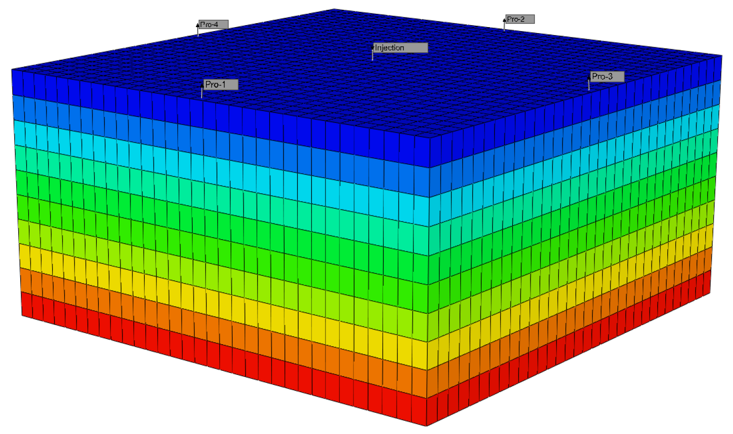
To verify the overall predictive ability of the model, this article uses two cases, including simulated data and on-site production data. The reservoir numerical simulation model data (Figure 4) are based on CMG simulation software (2021.10). The parameters of the numerical model (Case 1) are shown in

Table 2. Parameters of mechanism numerical model (Case 1).

Parameter	Value	Unit
Grid Size	320 × 320 × 10	m
Permeability	0.2 (P50)	mD
Porosity	0.08 (P50)	/
Oil Saturation	0.6	/
Simulation Years	10	/
Grid Layers	10	/
Depth	[2111, 2120]	m
Formation Pressure	23	MPa
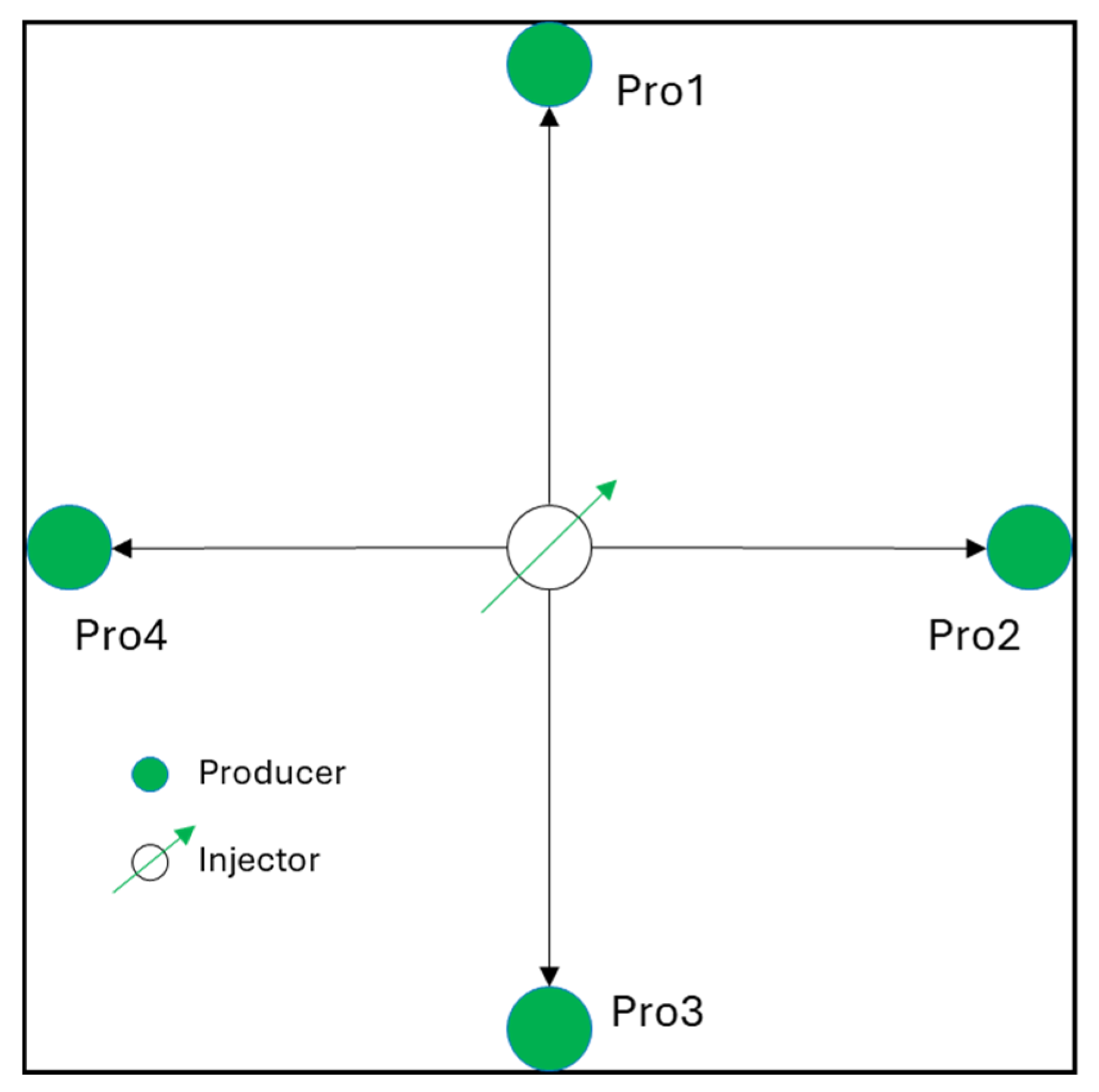
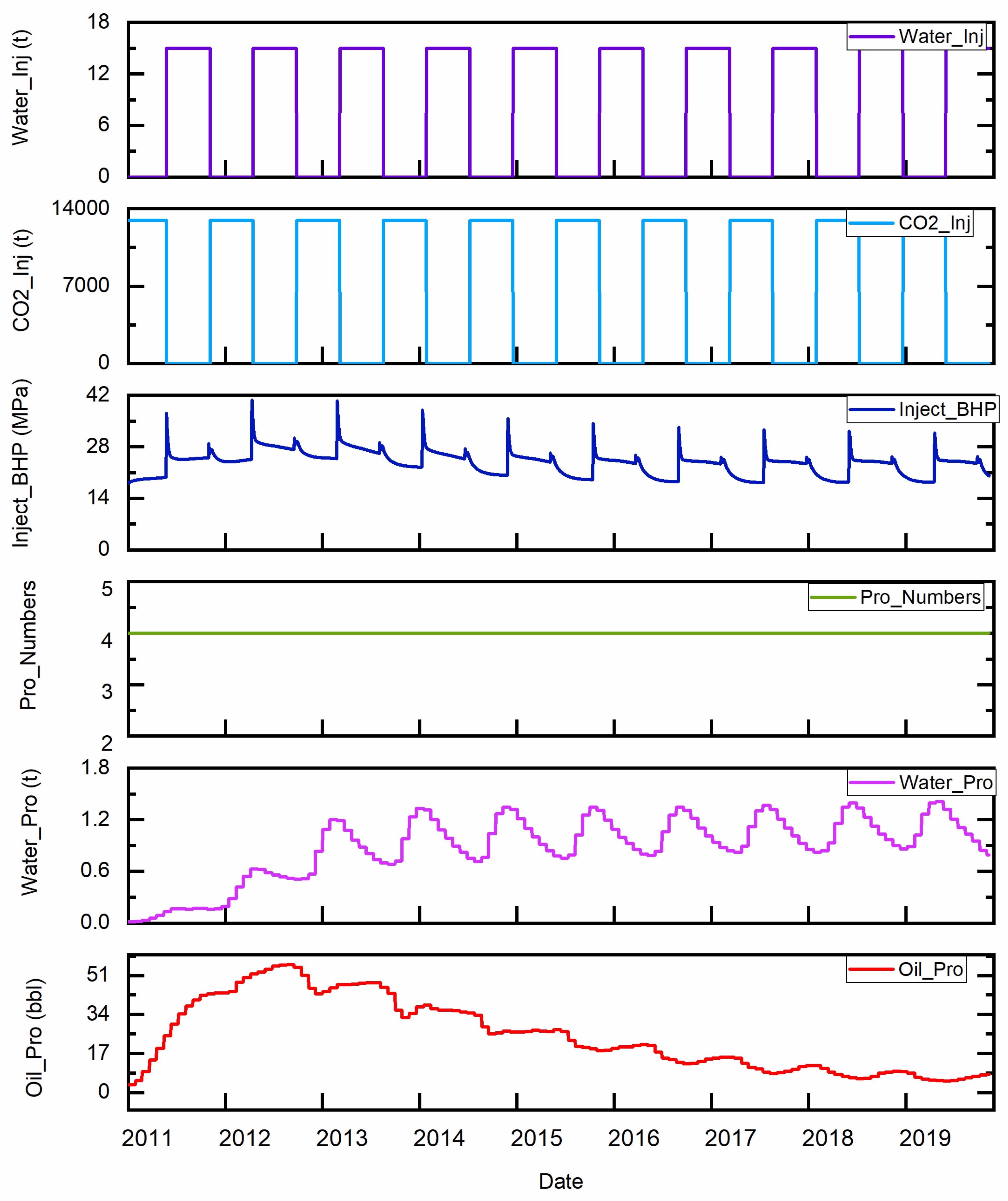
CO2 MMP	29	MPa

. It consists of five wells, with the central one being the injection well and the other four being production wells. The distance between the production well and the injection well is fixed at 160 m (Figure 5). It also includes 10 years of simulation results, encompassing oil production in the block, water injection and production, CO₂ injection, the normalization of well locations, the number of wells opened, and bottomhole pressure at injection locations (Figure 6).

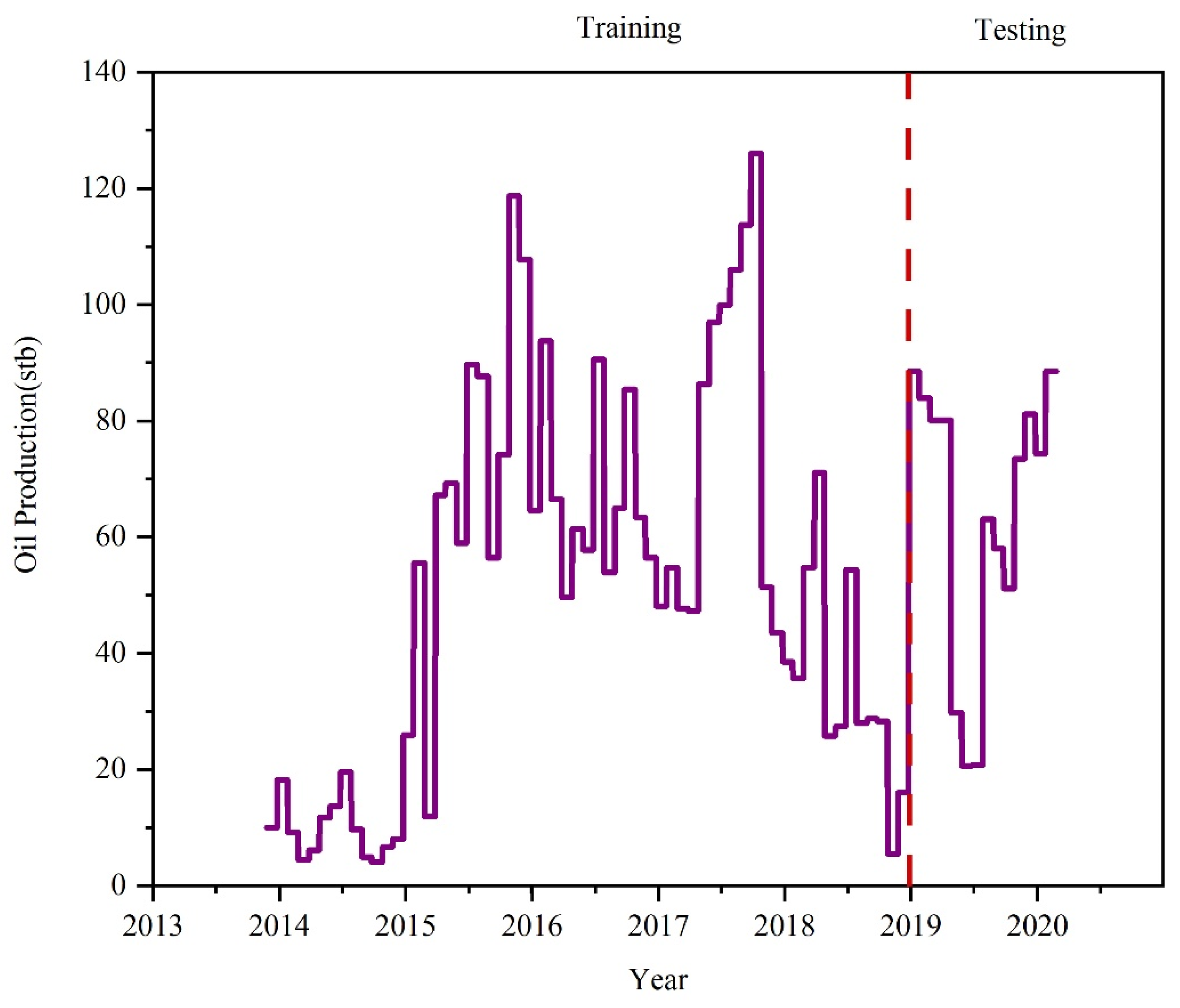
To ascertain the precision of predictive models concerning the production dynamics of individual oil wells under real-world conditions, another case is the Farnsworth Unit in Texas [4] dataset for validation purposes. It is based on a real-world oilfield, and the parameters of the oilfield data (Case 2) are shown in

Table 3. Parameters of real-world reservoir block model (Case 2).

Parameter	Value	Unit
Start Date	1 February 2005	/
End Date	1 February 2015	/
Average Porosity	0.1	/
Average Oil Saturation	0.55	/
Depth	[7550, 7950]	ft
Formation Pressure	25.1	MPa
CO2 MMP	31.9	MPa
Production Well Number	4	/
Injection Well Number	1	/

. It also has 10 years worth of results for training and testing, containing the oil production, the water injection and production, the CO₂ injection, the normalization of the well location, and the well-bottom pressure at the injection location.

In Case 2, to optimize the performance of the models, we adjusted the hyperparameters of each model, as shown in

Table 4. Hyperparameters of models in Case 2.

Hyperparameters	TCN	GRU	LSTM	KAN-LSTM	TCN-KAN	GRU-KAN
Batch Size	2	2	2	2	2	2
Window Size	3	2	2	2	3	2
Hidden KAN Layers	\	\	\	2	2	3
Kernel Numbers	3	\	\	\	2	\
Number of Residual Layers	2	\	\	\	1	\
Keneral Size	2	\	\	\	2	\
KAN Neuron Numbers	\	\	\	20	25	25

. By carefully tuning the learning rate, batch size, number of hidden units, and other key hyperparameters, we aimed to explore model configurations that are more suitable for the current dataset and task requirements.

C. Training and testing of the model

The selected input parameters (oil production, cumulative water and gas injection, and the well-bottom pressure at the injection location) are used for the model building.

D. Evaluation Criteria

In the field of prediction and forecasting, especially in production forecasting, the effectiveness of various forecasting methods is typically evaluated using a set of error-based metrics. These metrics offer a quantitative assessment of the accuracy and reliability of forecasts generated by different models. The most commonly used metrics include the root mean square error (RMSE), root mean square percentage error (RMSPE), and mean absolute percentage error (MAPE).

$$\begin{array}{c}RMSE=\sqrt{{\displaystyle \frac{1}{n}}{\displaystyle \sum _{i=1}^n{(y_i-{\widehat{y}}_i)}^2}}\\ RMSPE=\sqrt{{\displaystyle \frac{1}{n}}{\displaystyle \sum _{i=1}^n{(\frac{y_i-{\widehat{y}}_i}{y_i})}^2}}\\ \begin{array}{c}RMAE={\displaystyle \frac{1}{n}}{\displaystyle \sum _{i=1}^n\left|\frac{y_i-{\widehat{y}}_i}{y_i}\right|}\\ \mathrm{\Delta }={\displaystyle \sum _{i=1}^n(y_i-{\widehat{y}}_i)}\end{array}\end{array}$$

(3)

Additionally, the cumulative bias (Δ) is introduced as a metric to assess the systematic error or bias present in the model’s predictions. This metric is a pivotal indicator for evaluating the systematic errors or biases inherent in model predictions, especially in the context of yield forecasting. It quantifies the long-term cumulative bias by calculating the ratio of the deviation between the cumulative predicted value over many years and the true value. The calculation method for this metric is represented in Equation (3).

4. Results and Discussion

The test results of the reservoir numerical simulation mechanism model are in Figure 5. In the analysis of the plot, it is observed that the KAN-LSTM model exhibits superior performance. This observation suggests that within the context of the task at hand, the KAN-LSTM model demonstrates a more robust predictive capability in comparison to other models under consideration. In the comparative analysis of predictive models, it has been noted that the temporal convolutional network (TCN), when tasked with forecasting daily data, tends to produce more irregular predictions accompanied by higher error rates, which subsequently impacts the overall accuracy of the predictions. Meanwhile, long short-term memory (LSTM) and traditional gated recurrent unit (GRU) networks are capable of completing the prediction task, yet they exhibit certain biases in their forecasting.

Table 5. Summary of results in Case 1.

	KAN-LSTM	TCN	LSTM	GRU	TCN-KAN	GRU-KAN
RMSE	0.150	0.380	0.264	0.212	0.168	0.173
RMSPE (%)	2.466	22.66	12.239	8.102	3.051	3.987
MAPE (%)	2.021	15.80	8.936	5.213	2.964	3.103
Δ	11.51	1001.60	382.52	551.24	46.33	74.27

provides a comparative analysis of four common methods used in engineering neural network models—KAN-LSTM, GRU (gated recurrent unit), LSTM (long short-term memory), and TCN (temporal convolutional network)—based on their performance metrics for a specific prediction task. The metrics evaluated include the root mean square error (RMSE), root mean square percentage error (RMSPE), mean absolute percentage error (MAPE), and cumulative bias (Δ). Where applicable, each value is accompanied by a measure of variability to assess the consistency and reliability of the models’ predictions. 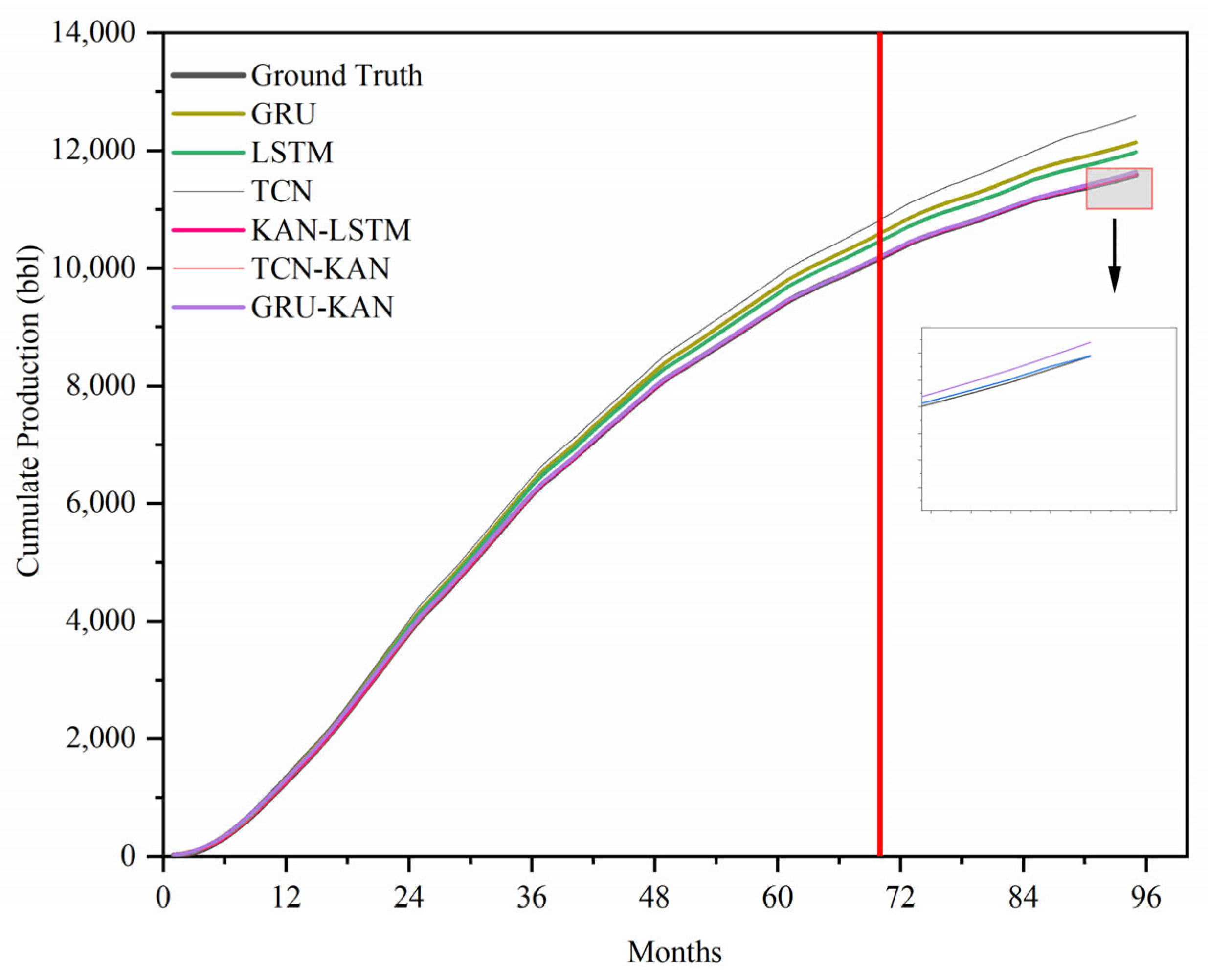Also, Figure 7 shows the cumulative yield prediction of these models.

The KAN-LSTM model achieves the lowest RMSE value of 0.150, indicating the most tightly distributed errors around the mean prediction. In contrast, the TCN model has the highest RMSE at 0.380, suggesting a larger spread of errors.

In terms of the RMSPE and MAPE, the KAN-LSTM model again demonstrates the lowest error values, at 2.466 and 2.021, respectively. Conversely, the TCN model exhibits the highest RMSPE and MAPE values, at 22.66 and 15.80, respectively. This indicates that the TCN model’s predictions, on average, deviate the most from the actual data points.

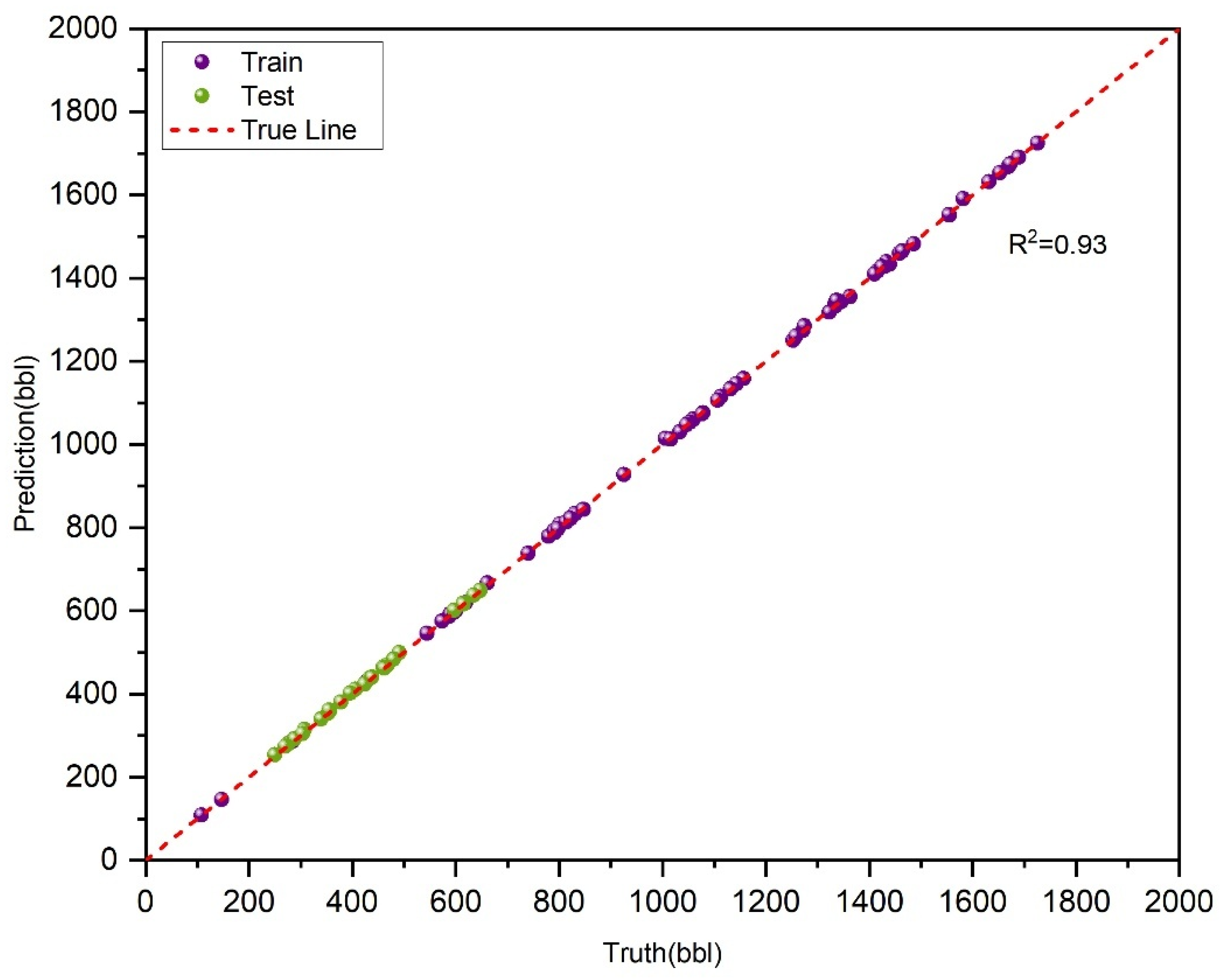
Additionally, the KAN-LSTM model shows the lowest cumulative bias (Δ) at 11.51, while the TCN model has the highest Δ value of 1001.60, highlighting a significant and variable bias in its predictions. Figure 8 shows the prediction and observation data of the KAN-LSTM model in the training and testing sections of Case 1.

In this case, the KAN-LSTM model outperforms all other models across every evaluation metric, demonstrating superior prediction accuracy and reliability for the task. Conversely, the TCN model shows the weakest performance, with higher errors and significant biases. This suggests that the TCN may not be well-suited for daily data prediction in this specific context.

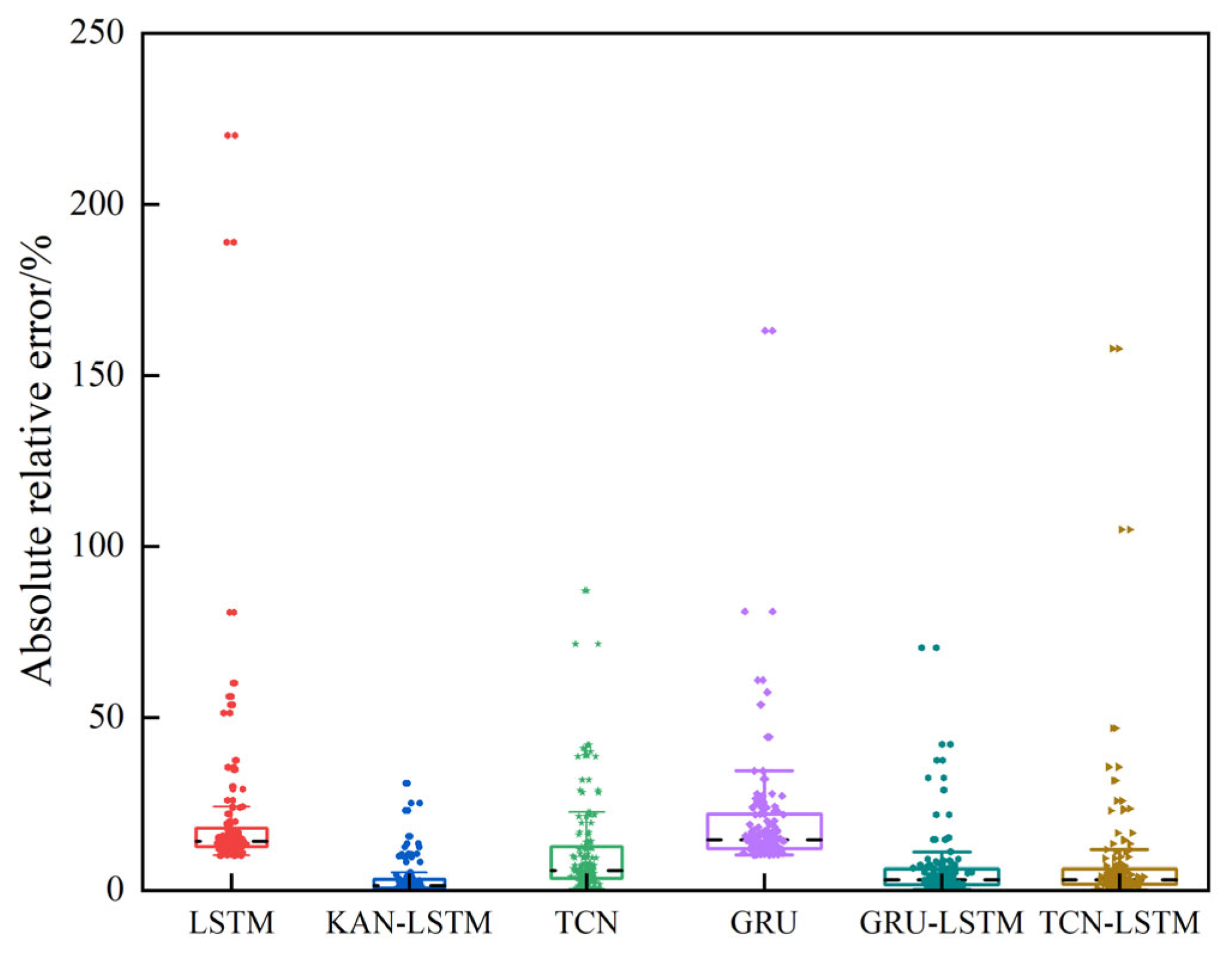
To verify its effectiveness in real-world scenarios, experiments are conducted on real-world oilfield data (Case 2). The real-world reservoir operation data are shown in Figure 9. Compared with other methods, KAN-LSTM also has the best predictive ability, which shows its robustness and effectiveness. The relative error distribution box plot of the test (Figure 10) set intuitively reflects the stability of the model prediction. Among them, the interquartile range (IQR) [33] clearly demonstrates the degree of dispersion of error data; the smaller the IQR, the more concentrated the error distribution predicted by the model and the higher the stability. On the contrary, the larger the IQR, the more dispersed the error distribution, and the stability of the model prediction is relatively weaker.

The indicators for Case 2 are shown in

Table 6. Summary of results in Case 2.

	KAN-LSTM	LSTM	GRU	TCN	TCN-KAN	GRU-KAN
RMSE	1.873	4.433	9.541	4.997	3.082	2.765
RMSPE (%)	6.822	22.724	48.518	19.064	8.032	10.242
MAPE (%)	3.700	10.188	16.416	11.678	6.789	8.786
Δ	2.11	9.417	−17.149	−8.705	4.75	5.357

. In Case 2, the median of the KAN-LSTM model is 0.150 and the remaining three non-hybrid network models are 0.441, 0.589, and 0.456, while the other two hybrid network models are 0.193 and 0.216. This indicates that 50% of the relative errors predicted by the KAN-LSTM model are less than 0.15%, which is the smallest value among the four models. In addition, the IQR of the KAN-LSTM model is 2.74, while the remaining three non-hybrid networks are 8.11, 8.77, and 10.09 and the two hybrid network models are 3.63 and 4.19, respectively.

Also, the KAN-LSTM model exhibits the lowest RMSE value of 1.873, indicating the tightest distribution of errors around the mean prediction. Conversely, the GRU model has the highest RMSE at 9.541, suggesting a larger spread of errors. In terms of the RMSPE and MAPE, the KAN-LSTM model again demonstrates the lowest error values of 6.822 and 3.700, respectively, while the LSTM model has the highest RMSPE and MAPE values at 48.518 and 16.416. This indicates that, on average, the TCN model’s predictions deviate the most from the actual data points. Additionally, the KAN-LSTM model shows the lowest cumulative bias (Δ) at 2.11, whereas the GRU model has the highest Δ value of −17.149, highlighting a significant and variable bias in its predictions.

5. Conclusions

In this study, a novel deep learning model KAN-LSTM was proposed for CCUS-EOR to accurately predict oil production. The KAN-LSTM model was applied to predict oil production in two cases, and the predicted results were compared with other common deep learning methods. The model assumes that the data used for training and testing are complete and accurate and that the geological conditions of the reservoir remain relatively stable during the study period. These assumptions may limit the model’s applicability in scenarios with data gaps or significant geological changes. There are conclusions to be drawn from the study.

(1) Model Development and Validation: By integrating the KAN with the time series network, we propose a KAN-LSTM model capable of extracting features from variables to accurately predict oil production. The model’s effectiveness has been verified using production data from numerical simulations of CO₂-EOR processes and the Farnsworth Unit dataset in Texas.

(2) Performance Comparison: Compared with other methods, the results highlighted several benefits of the proposed model, including the superior perception of multiple types of variables, forecasting performance and greater parameter efficiency. In analysis, it is shown that KANs consistently outperformed other methods in terms of lower error metrics and are able to achieve better results with lower computational resources.

(3) Practical Implications: Compared with the simulation result in Case 1, the proposed model eliminates the need for prior assumptions regarding reservoir type and properties. It enables faster forecasting by leveraging historical production data, thereby reducing the subjectivity associated with numerical simulations.

Given their effectiveness and efficiency, KANs not only appear to be a reasonable alternative to traditional artificial networks in oil production but also in traffic forecasting, weather forecasting, and some predictions based on environmental variable assistance. Owing to the scarcity of empirical data pertaining to shale oil and gas reservoirs, there exists an absence of research endeavors focused on the development of predictive models for these reservoirs, which are anticipated to possess significant value for future development.

However, the proposed model in this study has the following limitations and requires further research to enhance its future performance:

(1) Although the KAN-LSTM model demonstrates superior predictive performance, it requires a longer runtime compared to traditional time series models.

(2) This study did not account for the properties of different strata. Future work should incorporate diverse geological data to test the model and apply it across various oil fields, thereby improving its robustness.

(3) The KAN-LSTM model demonstrates superior predictive performance compared to other methods. However, it is important to note that the model’s performance is highly dependent on the completeness of the data. Additionally, the model assumes that the geological conditions of the reservoir remain relatively stable during the study period. Future work will focus on addressing these limitations by incorporating more advanced data preprocessing techniques and dynamic geological data to enhance the model’s robustness and adaptability.