An Improved SLAM Algorithm for Substation Inspection Robots Based on 3D Lidar and Visual Information Fusion

Abstract

Current substation inspection robots mainly use Lidar as a sensor for localization and map building. However, laser SLAM has the problem of localization error in scenes with similar and missing environmental structural features, and environmental maps built by laser SLAM provide more single-road information for inspection robot navigation, which is not conducive to the judgment of the road scene. For this reason, in this paper, 3D Lidar information and visual information are fused to create a SLAM algorithm applicable to substation inspection robots to solve the above laser SLAM localization error problem and improve the algorithm’s localization accuracy. First, in order to recover the scalability of monocular visual localization, the algorithm in this paper utilizes 3D Lidar information and visual information to calculate the true position of image feature points in space. Second, the laser position and visual position are utilized with interpolation to correct the point cloud distortion caused by the motion of the Lidar. Then, a position-adaptive selection algorithm is designed to use visual position instead of laser inter-frame position in some special regions to improve the robustness of the algorithm. Finally, a color laser point cloud map of the substation is constructed to provide more road environment information for the navigation of the inspection robot. The experimental results show that the localization accuracy and map-building effect of the VO-Lidar SLAM algorithm designed in this paper are better than the current laser SLAM algorithm and verify the applicability of the color laser point cloud map constructed by this algorithm in substation environments.

1. Introduction

Substation inspection [1,2] is carried out to ensure the normal operation of substation equipment. As one of the effective measures of smart grids, in recent years, intelligent inspection robots have begun to enter substations and other electric power places. Traditional manual inspection has been gradually replaced by robotic inspection methods. As is known to all, for an inspection robot, the primary task of substation inspection is to realize autonomous navigation. The current inspection robot navigation method mainly involves magnetic navigation, but a method exists that involves a magnetic track-laying workload. The path is fixed and is not easy to change, among other shortcomings. With the development of artificial intelligence, as one of the key technologies in the field of autonomous driving and augmented reality, simultaneous localization and mapping (SLAM) [3,4] technology has been widely used in the field of intelligent robotics.

SLAM technology can be divided into three categories according to the type of sensor used, namely, laser SLAM, vision SLAM, and multi-sensor fusion SLAM. Current substation inspection robot SLAM technology research is mainly focused on laser SLAM technology [5,6] because laser SLAM information acquisition is accurate, has a simple error model, indoor and outdoor work are stable, the theory is relatively mature, and there are more abundant landing products and engineering applications. However, current laser SLAM technology has the disadvantages of single sensor information, not rich enough information to build the environment map, and poor localization in the environment, such as the degradation of structural features and other regions, which is not conducive to the inspection robot’s judgment of the road and environment. Visual sensors can obtain rich environmental information. They are small in size, low in price, and easy to install and integrate but are easily affected by environmental conditions, and their stability and real-time are poor. So, it is difficult to obtain the application of single visual SLAM in engineering. Therefore, it is of great significance to study a SLAM algorithm that is applicable to substation inspection robots [7,8] to improve the positioning and map building accuracy of inspection robots, to build a more information-rich substation environment map, to provide more effective road environment information for the navigation of inspection robots, and to improve the safety and intelligence of substation inspection robots.

In order to solve the problems of current laser SLAM technology being relatively single in obtaining sensor information, the information of the constructed environment map not being rich enough, the localization not being good, and so on, in this paper, a SLAM algorithm is proposed for substation inspection robots that fuses 3D Lidar information with visual information. The algorithm uses image feature points combined with laser point 3D information to calculate the true position of the image feature points in space, restore the scale of monocular visual localization, and use the laser position and visual position with interpolation to correct the point cloud aberration of the Lidar due to motion. At the same time, a position-adaptive selection algorithm is designed to replace the laser inter-frame position with the visual position in the area where the environmental structural features are not obvious or similar to improve the robustness of the algorithm. The robustness of the algorithm is improved by replacing the laser inter-frame position with the visual position in areas where environmental structure features are not obvious or similar. Considering the demand for substation environment maps for inspection robot navigation, this paper fuses the image pixel information and the position information of laser points to construct a color laser point cloud map of a substation, which provides more useful environment information for inspection robot navigation. The experimental results show that the positioning accuracy and map building effect of the VO-Lidar SLAM algorithm designed in this paper are better than the current laser SLAM algorithm and verify the applicability of the color laser point cloud map constructed by this algorithm in a substation environment.

The contributions of this paper are summarized below.

(1)

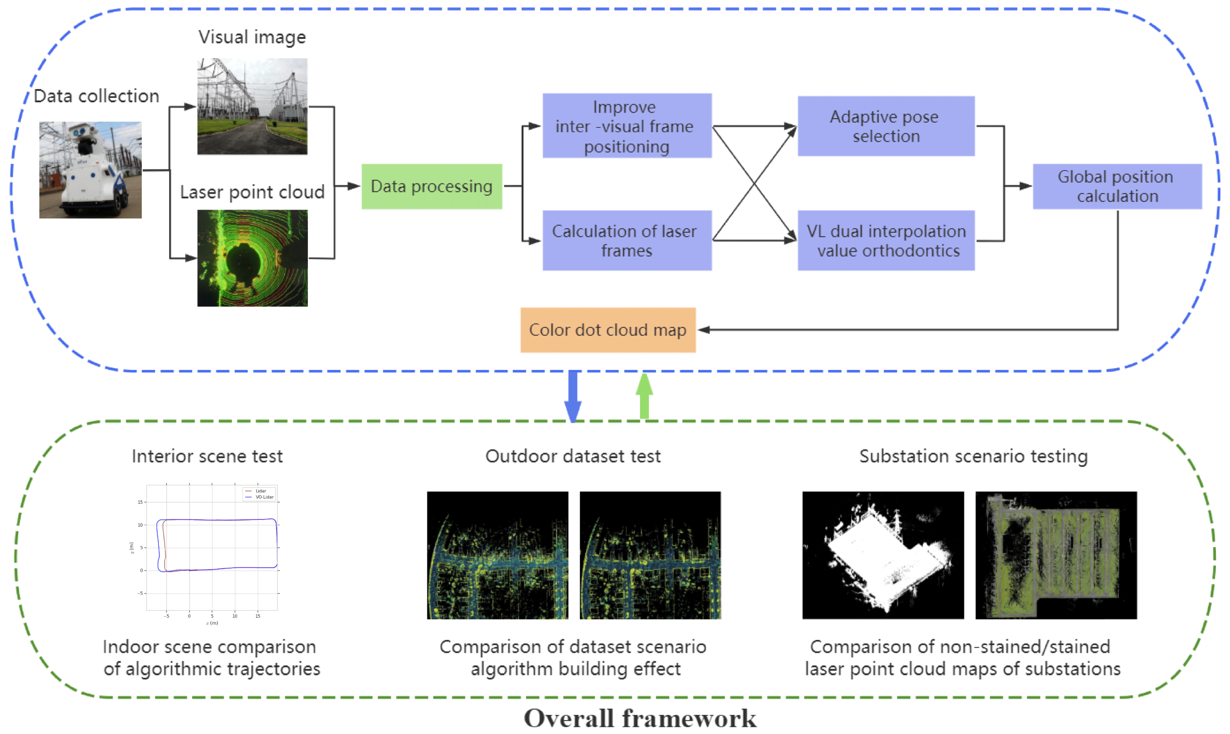
In this paper, a 3D laser and vision fusion SLAM algorithm for inspection robots is proposed. The algorithm combines image feature points and 3D laser point position information, uses the laser position and visual position with interpolation, applies the position-adaptive selection method to improve the positioning accuracy and robustness of the algorithm, and finally, constructs a color laser point cloud map of the substation.

(2)

The algorithm in this paper was combined with a substation inspection robot and tested in real sites to verify its applicability in real environments. A substation inspection robot equipped with 3D Lidar and vision sensors was used to experimentally test the inspection robot VO-Lidar SLAM algorithm proposed in this paper through three different environments, namely, an indoor scene, an outdoor dataset, and a substation.

The rest of this paper is organized as follows. Section 2 presents the work related to this paper. Section 3 describes the methodology proposed in this paper in detail. Section 4 provides an experimental validation of the methodology proposed in this paper. Finally, Section 5 presents the conclusions of this paper and future work.

2. Related Works

Substation inspection is an effective measure used to ensure the normal operation of substation equipment. In recent years, with the rapid development of artificial intelligence, a large number of intelligent inspection robots have appeared in substations. As one of the key technologies in the field of autonomous driving and augmented reality, SLAM technology has been widely used in the field of intelligent robots [9]. At present, the SLAM technology used in inspection robots can be mainly divided into two classes: laser SLAM and vision SLAM.

On the one hand, early laser SLAM was solved by Kalman filtering or particle filtering. Montemerlo et al. [10,11] combined the two methods for localization and extended Kalman filtering to update the map, which improved the efficiency of the SLAM process. In 2014, Zhang et al. [12,13] proposed a real-time localization and 3D laser point cloud building algorithm, which improves both localization accuracy and real-time performance. In October 2016, Google released an open-source laser SLAM algorithm called Cartographer [14], which uses graph optimization and closed-loop detection to improve the accuracy of the algorithm’s positioning and map construction. However, there are still some shortcomings in laser SLAM. Firstly, the color of spatial objects cannot be obtained by laser radar. Secondly, it is difficult for laser radar to receive reflection data in an open environment. The structural characteristics of the data received in a structurally similar environment are basically the same, which can cause laser frame-to-frame matching errors. In particular, ice or snow on roads will lead to changes in the characteristics of the laser reflections, affecting the localization accuracy. Therefore, in terms of substation environments, single-laser SLAM can experience localization errors in scenes with similar or missing environmental structural features. In addition, the established substation map contains less environmental information, which is not conducive to the recognition of the road environment by the inspection robot.

On the other hand, as early visual SLAM was limited by computational performance, its localization accuracy and real-time performance were poor. Nowadays, with the improvements in graphical processing units, the cost of sensors is becoming lower and lower, which is beneficial for obtaining rich visual information. Current mainstream visual SLAM algorithms are based on the graph optimization framework. Among them, the most representative one is the Parallel Tracking and Mapping (PTAM) algorithm [15], which divides localization and mapping into two independent tasks. The tasks are parallelly processed in two threads: one thread is used to process the motion of the sensors, and the other is used to generate the 3D mapping of the feature points. In Spain, Raulmur et al. [16,17] proposed ORB-SLAM (Oriented Brief SLAM) based on the PTAM algorithm. The algorithm adopts ORB feature points and closed-loop detection, which achieves better results in terms of processing efficiency, localization, and map building accuracy. The above two algorithms build sparse maps, which cannot restore the real environment and are not very helpful for mobile robot navigation. Therefore, RGB-D SLAM [17,18] uses a depth camera to obtain depth of color pixels and calculates the camera’s position according to the iterative closest point (ICP) algorithm, which realizes dense 3D reconstruction in small indoor scenes. In addition, Kinect-Fusion [19] uses only depth information for localization and map construction, representing the first algorithm to realize the real-time construction of dense 3D point cloud maps by a Kinect camera. In addition, LSD-SLAM [20], a binocular SLAM algorithm proposed by Engel et al. in 2014, adopts a direct method to process the image pixels, which can not only calculate the camera’s bit position but also construct semi-dense maps for large-scale environments [21]. However, the large amount data processed directly on the image pixels leads to the algorithm demonstrating low real-time performance. As a result, neither single-laser SLAM nor single-vision SLAM are conducive to the judgment of the environment by inspection robots. Thus, in terms of the characteristics of inspection robots, a 3D Lidar and vision fusion SLAM algorithm (VO-Lidar SLAM) is developed for the environmental mapping of substation environments by inspection robots in this paper.

3. Framework of the Study

In this section, in terms of a substation environment and the characteristics of inspection robots, a 3D Lidar and VO-Lidar SLAM algorithm is developed. The algorithm fuses two mainstream sensors, Lidar and a visual camera. To address the problem of localization errors in laser SLAM, it integrates vision localization with Lidar localization technology. Moreover, it fuses image pixel information and laser point cloud information to construct a color laser point cloud map of the substation, which provides more road scene information for inspection robot navigation. The general framework of the SLAM algorithm for 3D Lidar and vision fusion for use by inspection robots in substations is shown in Figure 1.

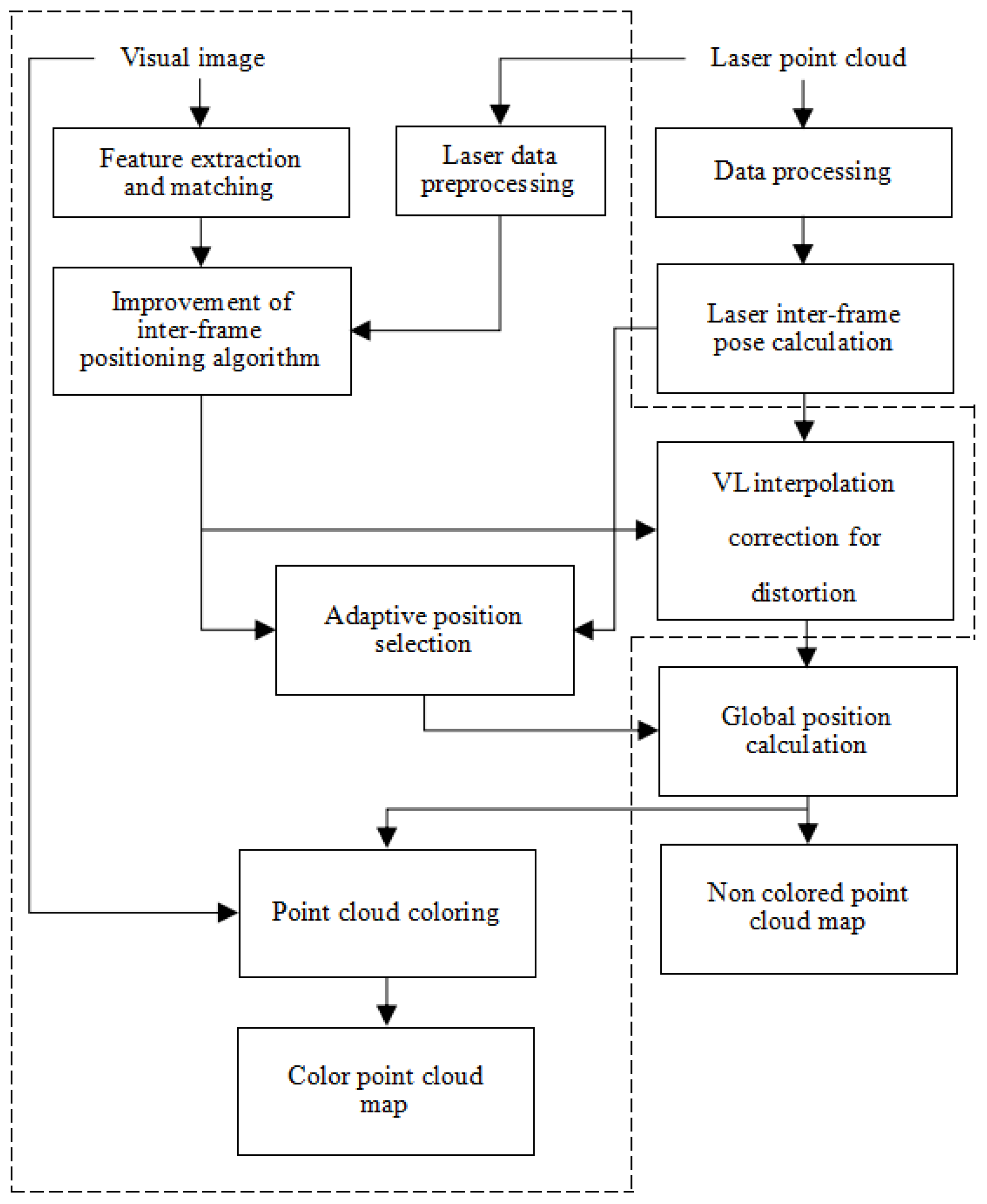
3.1. Algorithm Fusion Framework

The general framework of the VO-Lidar SLAM algorithm for inspection robots in this section is shown in Figure 2. On the one hand, considering an inspection robot’s all-weather inspection characteristics, the front-end of the VO-Lidar SLAM algorithm consists of a vision localization algorithm and a laser localization algorithm, which are processed in parallel to compute inter-frame positional transformations. Thus, when there are laser localization errors or a lack of light, the algorithm can achieve more accurate localization of the inspection robot. The visual localization of the proposed algorithm mainly consists of three parts: image feature extraction and matching [22,23], laser data preprocessing, and an improved inter-frame localization algorithm. Meanwhile, the laser inter-frame localization algorithm also consists of three parts: laser data processing, laser interframe position computation, and laser visual bi-interpolation for correcting point cloud aberrations. On the other hand, the main functions of the back-end of the VO-Lidar SLAM algorithm mainly include laser vision position adaptive selection, global position calculation, and the construction of both color and non-color laser point cloud maps.

3.2. Improved Visual Interframe Localization

In this section, to address the scalability issue of monocular cameras, the depth information of the image feature points is first calculated by combining the spatial position information of the laser points. Then, the position information of the robot is calculated by 3D-3D feature point matching.

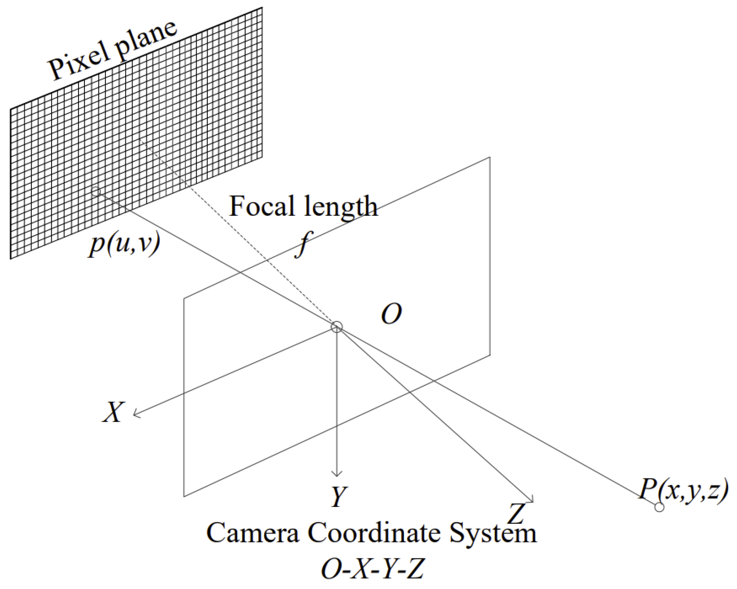
3.2.1. Depth Calculation of Feature Points Based on the Laser Projection Method

As is known to all, image feature points and Lidar point clouds belong to different coordinate systems. This algorithm sets the monocular camera’s coordinate system as the robot’s coordinate system (ignoring the error between the robot’s coordinate system and the sensor’s coordinate system).

The horizontal scanning range of the 3D Lidar is 360 degrees, but the horizontal field of view of the camera is less than 180 degrees, which means that it can only observe the environmental information in front of the robot. As a result, it is necessary to preprocess the Lidar point cloud data before feature point depth calculation. The pre-processing process is as follows:

(1)

Select the laser points within 180 degrees in front of the robot.

(2)

Convert these laser points from the Lidar coordinate system to the camera’s coordinate system.

The conversion formula is shown in Equation (1).

$$P=\left[\begin{array}{c}X\\ Y\\ Z\end{array}\right]=\left[\begin{array}{ccc}{r}_{S1}& r_{S2}& r_{S3}\\ r_{S4}& r_{S5}& r_{S6}\\ r_{S7}& r_{S8}& r_{S9}\end{array}\right]\ast \left[\begin{array}{c}{X}_L\\ Y_L\\ Z_L\end{array}\right]+\left[\begin{array}{c}{t}_{Sx}\\ t_{Sy}\\ t_{Sz}\end{array}\right]$$

(1)

where $P_L(X_L,Y_L,Z_L)$ are the laser point coordinates under the Lidar coordinate system, $P$ is the laser point coordinates converted to the camera’s coordinate system, and $R_S$ and $t_S$ are the rotation and translation matrices from the Lidar coordinate system to the camera’s coordinate system, which are obtained by sensor calibration. The change in the laser point position before and after the conversion is shown in Figure 3, where the colored point cloud is the laser points under the laser’s coordinate system, and the white point cloud is the laser points converted to the camera’s coordinate system.

After the laser points are converted, the laser projection method [24] is used to combine the image feature points with the 3D laser point position information to calculate the true depth of the feature points. The core idea of the laser projection method is to project the 3D laser points and 2D image feature points onto the same plane. Then, the method deduces the position of the image feature points relative to the laser points according to the positional relationship between the laser projection points and the image projection points on the plane.

The specific calculation method of the laser projection method refers to Figure 4. The image feature point $\left(u,v\right)$ on the pixel plane is back-projected to the normalization plane (z = 1) to obtain the point $q\left(x,y,1\right)$ through the camera’s internal reference $(f_x,c_x,f_y,c_y)$, and the conversion formula is shown in Equation (2).

$$x={\displaystyle \frac{u-c_x}{f_x}}, y={\displaystyle \frac{v-c_y}{f_y}}$$

(2)

Then, the laser point P is projected onto the normalized plane of the camera coordinate system to obtain the point $p\left(X/Z,Y/Z,1\right)$; for the image feature point q on the normalized plane, the three closest laser projection points $p_1$, $p_2$, and $p_3$ are looked for, where their actual positions in space are $P_1$, $P_2$, and $P_3$; from the optical center O of the camera, a ray is drawn out through the image feature point q, and the plane composed of the three laser points in space $P_1{P}_2{P}_3$ intersects the point $Q(X,Y,Z)$, where the intersection point Q is the actual position of the image feature point q in space. The actual position of the image feature point q in space and the Q point coordinates of the three points, $P_1{P}_2{P}_3$, constitute the plane Equation $f(X,Y,Z)=0$, where $X=xZ$, $Y=yZ$ and where x and y are the q point coordinates; the Equation can be solved using the Z coordinates of Q, i.e., the depth value.

3.2.2. Visual Inter-Frame Position Calculation

Visual inter-frame position calculation is carried out to match the feature points on two consecutive frames, and the change in the position of the camera between the two frames is calculated by the matched feature point pairs. After calculating the depth information of the feature points by the laser projection method described above, two sets of matched 3D point sets are obtained, and the change in the camera’s position is then calculated by ICP.

For two consecutive visual images A and B, the corresponding sets of 3D matching points in the two images are $A(a_i)$ and $B(b_i)$, and the inter-frame bitmap is calculated by 3D-3D as follows:

First, the error of a single point pair is defined, as shown in Equation (3):

$$\forall i,e_i=b_i-(R{a}_i+t)$$

(3)

where R and t are the translation and rotation matrices from A to B, and $a_i$ and $b_i$ are the matched point pairs.

The least squares problem is constructed, as shown in Equation (4), solving for R and t, such that the sum of the squares of the transformation errors is minimized for all pairs of points:

$$\underset{R,t}{\min }E={\displaystyle \frac{1}{2}}{\displaystyle \sum _{i=1}^n}{||b_i-(R{a}_i+t)||}^2$$

(4)

The coordinates of the centers of the two point sets $A(a_i)$ and $B(b_i)$ are calculated according to Equation (5):

$$a={\displaystyle \frac{1}{n}}{\displaystyle \sum _{i=1}^n{a}_i,b=}{\displaystyle \frac{1}{n}}{\displaystyle \sum _{i=1}^n{b}_i}$$

(5)

Equation (5) is brought into Equation (4) and expanded to obtain Equation (6):

$$\begin{array}{ll}{\displaystyle \frac{1}{2}}{\displaystyle \sum _{i=1}^n||b_i-(R{a}_i+t)|{|}^2}& ={\displaystyle \frac{1}{2}}{\displaystyle \sum _{i=1}^n||(b_i-b-R(a_i-a)})+(b-Ra-t)|{|}^2\\ & ={\displaystyle \frac{1}{2}}{\displaystyle \sum _{i=1}^n(||b_i-b-R(a_i-a)|{|}^2+||b-Ra-t}|{|}^2\\ & +2(b_i-b-R(a_i-a))(b-Ra-t)\end{array}$$

(6)

As:

$${\displaystyle \sum _{i=1}^n(}{b}_i-b-R(a_i-a))=0$$

(7)

So, the simplified result of Equation (4) is shown in Equation (8):

$$\underset{R,t}{\min }E={\displaystyle \frac{1}{2}}{\displaystyle \sum _{i=1}^n||(b_i-b-R(a_i-a)|{|}^2}+||b-Ra-t|{|}^2$$

(8)

In Equation (8), the right side of the equals sign are the two square terms, the left side of the square term is only related to the rotation matrix R, the two point sets of the center point coordinates b and a are fixed. The equation is solved for the left side of the square term value for the smallest R, and then, based on the value of R, the value of t is obtained to minimize the error; the calculation process is as follows:

The difference between the coordinates of each point and the center point is calculated according to Equation (9):

$$a_i^{\prime }{=\mathrm{a}}_i-a,b_i^{\prime }{=\mathrm{b}}_i-b$$

(9)

Based on the above analysis, solving Equation (8) can be preceded by solving Equation (10):

$$R^{*}=\arg \underset{R}{\min }{\displaystyle \frac{1}{2}}{\displaystyle \sum _{i=1}^n||b_i^{\prime }-R{a}_i^{\prime }|{|}^2}$$

(10)

Expanding the error term about the rotation matrix R yields Equation (11):

$${\displaystyle \frac{1}{2}}{\displaystyle \sum _{i=1}^n||b_i^{\prime }-R{a}_i^{\prime }|{|}^2}={\displaystyle \frac{1}{2}}{\displaystyle \sum _{i=1}^n(b_i^{\prime T}{b}_i^{\prime }+a_i^{\prime T}{R}^{T}R{a}_i^{\prime }-2b_i^{\prime T}R{a}_i^{\prime })}$$

(11)

The first term of the above equation is independent of R. The rotation matrix satisfies $R^{T}R=I$ [25], such that $M={\displaystyle \sum _{i=1}^n{a}_i^{\prime }}{b}_i^{\prime T}$, which reduces the solution function with respect to R to Equation (12):

$${\displaystyle \sum _{i=1}^n-(b_i^{\prime T}R{a}_i^{\prime })}=-tr(RM)$$

(12)

Here, the singular value decomposition [26,27] is used to solve the above equation, where M is a 3 × 3 matrix, i.e., the singular-value decomposition of M, and the expression is shown in Equation (13):

$$M=U{\displaystyle \sum V^T}$$

(13)

The rotation matrix R is shown in Equation (14):

$$R=U{V}^T$$

(14)

The translation matrix t is solved for using Equation (15):

$$t=b-Ra$$

(15)

After obtaining the rotation and translation matrices between the two frames, the successive inter-frame transformation matrices are accumulated according to Equation (16) to obtain the camera’s, i.e., the robot’s moving trajectory and the positional information at any moment:

$$T=T_n\cdot T_{n-1}\dots T_2\cdot T_1$$

(16)

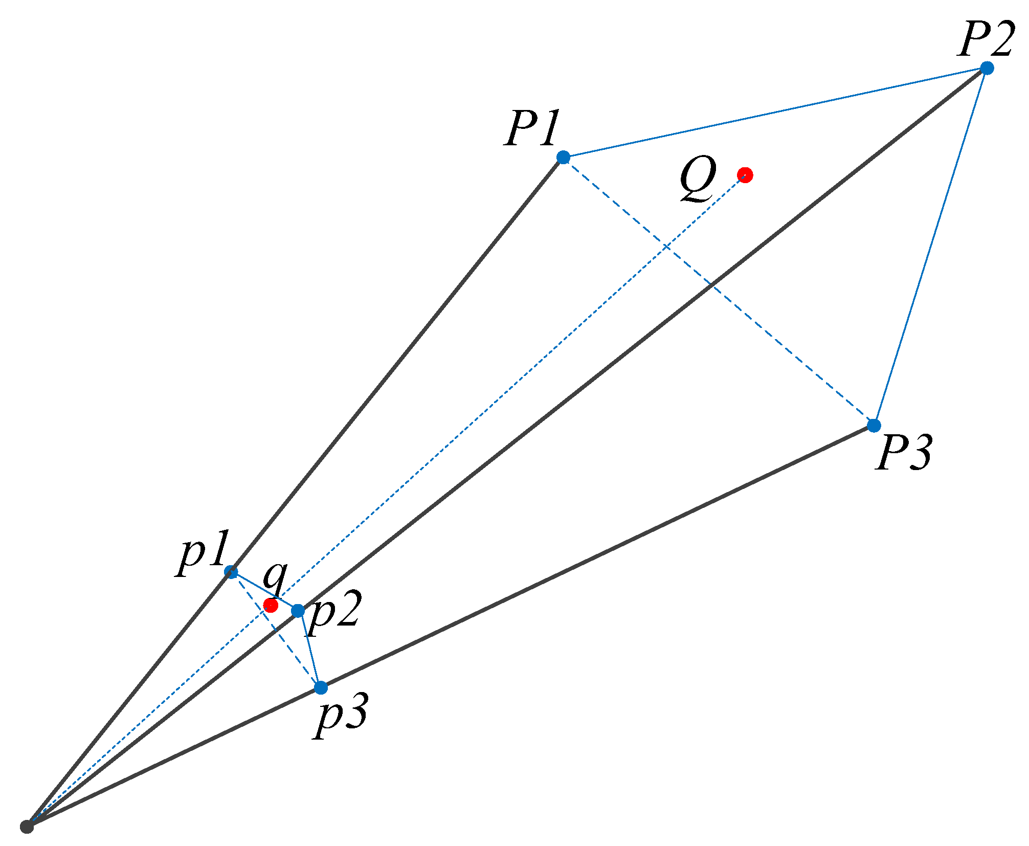
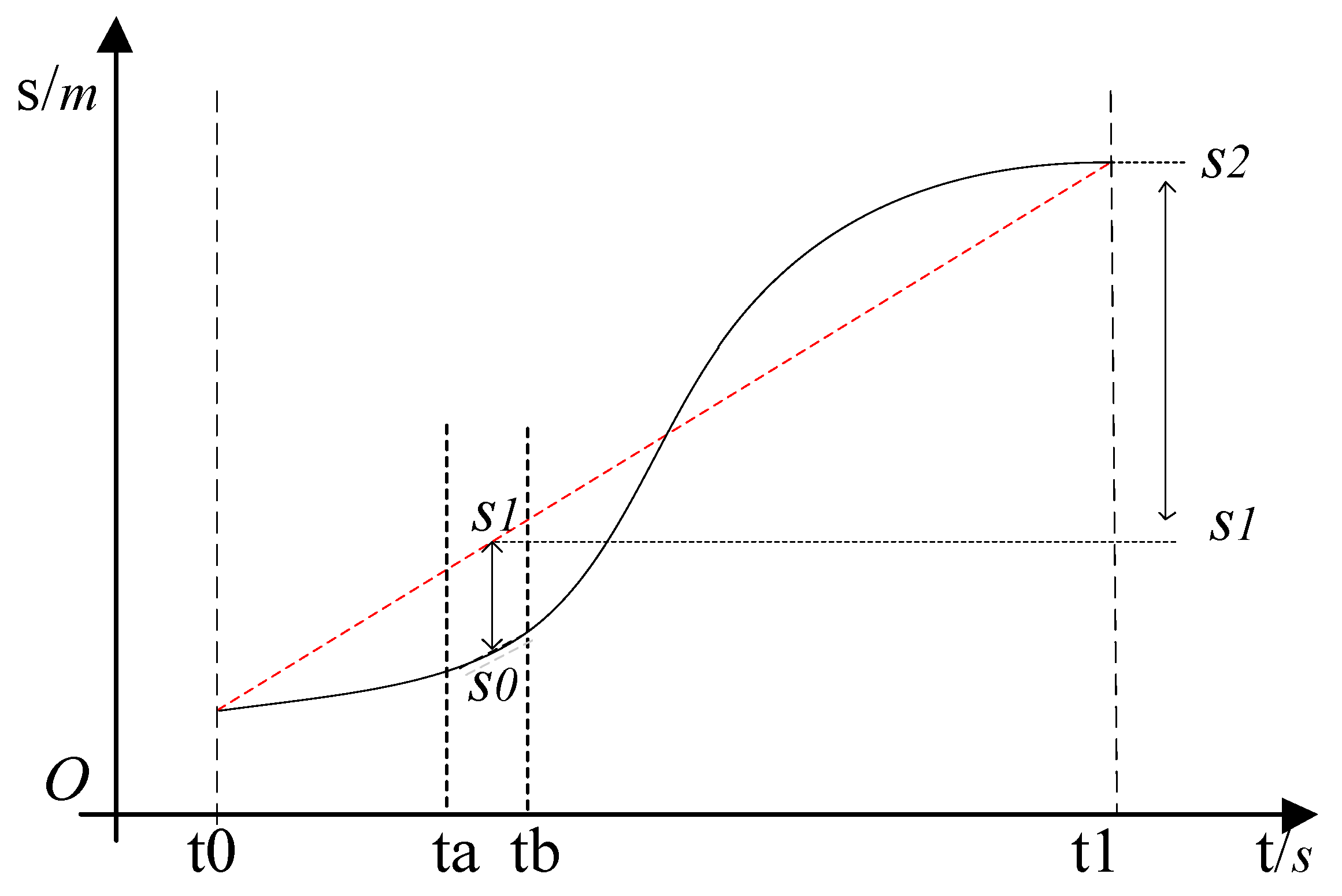
3.3. Laser Vision Double Interpolation to Correct Point Cloud Distortion

Lidar disregards the scan period when recording data, and it treats the timestamps of all laser points within the same frame of data as a unified point in time. Ignoring the scanning period causes distortion in the collected laser point positions, which affects the accuracy of the point cloud matching between laser frames as well as the accuracy of the laser point cloud and map matching.

To solve the problem of point cloud aberration, this section combines Lidar inter-frame position information with vision inter-frame position information to correct the laser point cloud aberration by means of cooperative interpolation.

Figure 5 shows the motion curve of the Lidar displacement S with time t. The detailed calculation process of the laser point cloud distortion correction is as follows.

1. Visual position interpolation for handling non-uniform motion.

For any laser point P obtained during the (ta, tb) time period, θ is the horizontal scanning angle of point P. The scanning time of point P is calculated according to Equation (17) (the scanning period is 0.1):

$$t=(\theta /2\pi )\ast 0.1+t0$$

(17)

Approximating the motion of the Lidar in the time period of (ta, tb) as a uniform motion, the Lidar obtains the point $P(x,y,z)$ at S₀, the visual position at the time period of (ta, tb) is linearly interpolated, as shown in Equation (18), the corresponding position transformation matrix is calculated for the time period of t, and $\overline{T}$ is the vector form corresponding to the transformation matrix T:

$$T_t^V~{\overline{T}}_t^V={\overline{T}}_{(tb,ta)}^V{\displaystyle \frac{(t-ta)}{(tb-ta)}}$$

(18)

The coordinates of point P relative to the laser scanning start position are calculated according to Equation (19):

$$P_{t0}={(T_t^V{T}_{(ta,t0)}^V)}^{-1}\oplus P$$

(19)

Linear interpolation of the visual position according to uniform motion during the (t0, t1) time period is performed to calculate the position transformation matrix corresponding to moment t. The calculation formula is shown in Equation (20):

$$T_t^V\prime ~{\overline{T}}_t^V\prime ={\overline{T}}_{(t1,t0)}^V{\displaystyle \frac{(t-t0)}{(t1-t0)}}$$

(20)

The coordinates of point P are calculated with respect to S₁ according to Equation (21):

$$P\prime =T_p^{\prime V}\oplus P_{t0}$$

(21)

where T’_p^V is the position transformation matrix corresponding to point P at moment t, and P_t0 are the coordinates of point P relative to the laser scanning start position.

Through the above process, the coordinates of point $P^{\prime }$ are equivalent to the actual coordinates of point P at S₁ when the Lidar is moving at a constant speed.

2. Laser position interpolation to handle uniform motion.

After compensating the Lidar motion to uniform motion by visual position interpolation, the laser point cloud aberration is corrected according to a uniform motion model. Due to the large amount of aberration and the poor stability of visual sensors, considering the robustness of the algorithm, a more stable laser position is interpolated here. The position transformation matrix corresponding to each laser point is calculated to obtain the coordinates of the laser point relative to the end position of the scan.

A linear interpolation of the laser position is performed within (t0, t1) according to Equation (22) to compute the corresponding position transformation matrix at time t. The position transformation matrix is then computed as follows:

$$T_t^L~{\overline{T}}_t^L={\overline{T}}_{(t1,t0)}^L{\displaystyle \frac{(t-t0)}{(t1-t0)}}$$

(22)

The coordinates of point P relative to the end position of the scan are calculated by Equation (23):

$$P_{t1}=T_{(t1,t0)}^L{(T_t^L)}^{-1}\oplus P\prime$$

(23)

$P_{t1}$, obtained by laser vision bi-interpolation to correct the aberration, is the position of point P relative to the Lidar at the end of scanning, the above aberration correction is carried out for all the laser points in the frame, and each frame of the corrected laser point cloud corresponds to the results obtained by the Lidar scanning after remaining stationary for one week at the end position.

In order to verify the enhancement effect of the laser SLAM algorithm localization accuracy after processing the laser point cloud distortion, the algorithm localization accuracy before and after the distortion correction was tested by using loopback experiments. The error calculation formula is shown in Equation (24):

$$error=100\times {\displaystyle \frac{\left|A_{(x,y,z)}-B_{(x,y,z)}\right|}{d}}$$

(24)

where $A_{(x,y,z)}$ are the coordinates of the starting point of the inspection robot, $B_{(x,y,z)}$ are the position of the inspection robot estimated by the algorithm when the inspection robot returns to the starting point, and d is the length of the motion trajectory of the inspection robot calculated by the algorithm. The results of the localization error before and after the aberration correction of the laser SLAM algorithm measured by the loopback experiments are shown in

Table 1. Laser SLAM localization error before and after aberration correction.

Arithmetic	Length d(M)	Starting Point Coordinates A (x, y, z)	End Point Coordinates B (x, y, z)	Positioning Error %
Lidar	72.477	(0, 0, 0)	(1.064, 0.199, 0.085)	1.498
After distortion correction	72.563	(0, 0, 0)	(0.957, 0.171, 0.076)	1.344

, from which it can be seen that the localization accuracy of the laser SLAM algorithm after point cloud aberration correction was better than that of the original laser SLAM algorithm, which verifies the validity of the aberration correction method.

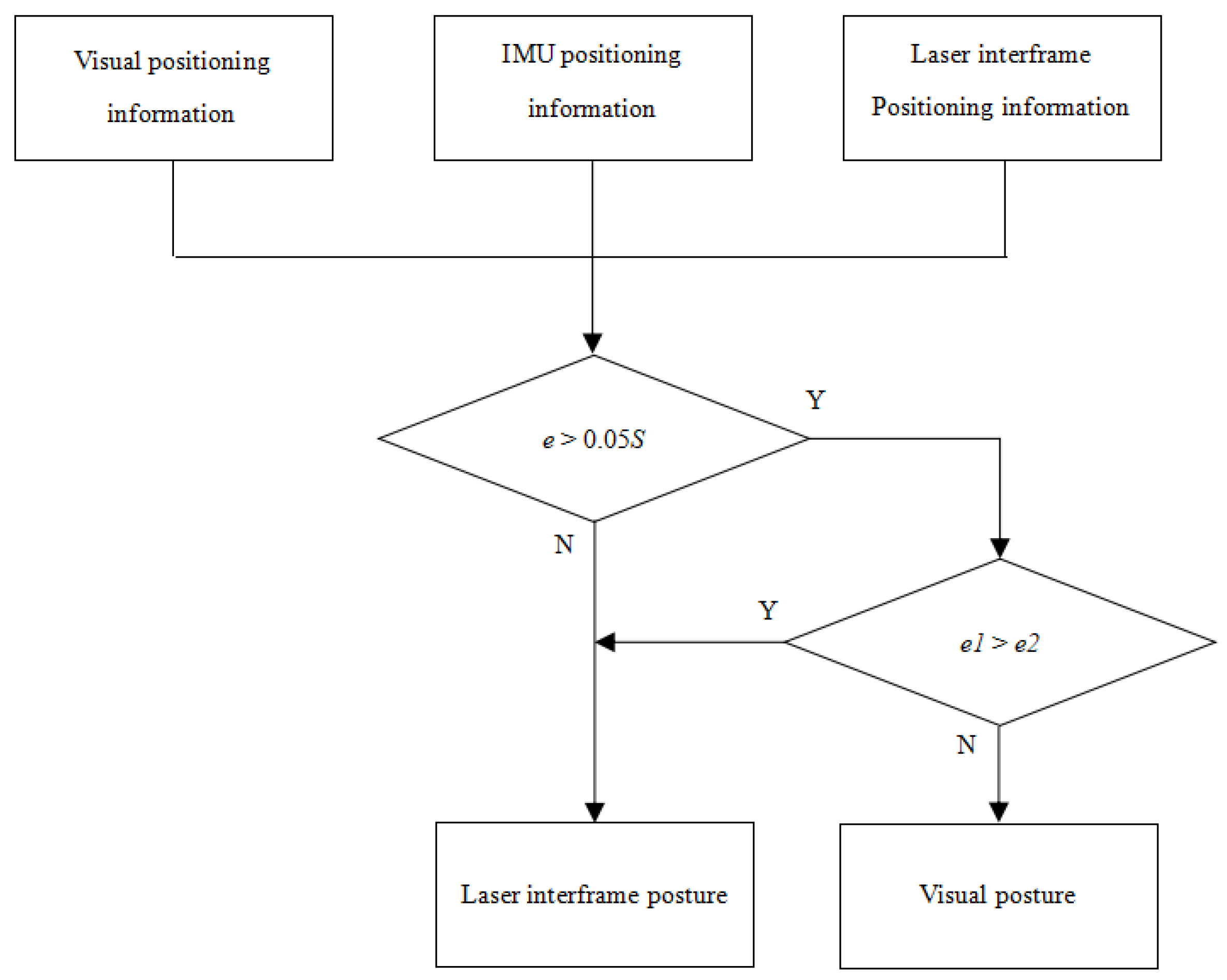
3.4. Laser Vision Position Adaptive Selection Methods

When the robot moves in areas with similar or missing environmental structural features, such as long corridors, aisles, and squares, several issues can arise. Firstly, due to the similarity of structural features in the data collected by Lidar, laser SLAM encounters difficulties in laser inter-frame matching. This, in turn, leads to localization errors. These errors provide incorrect initial values for the back-end position optimization process. Consequently, the back-end localization and mapping errors increase, and in severe cases, they may even result in mapping failures.

In order to solve the above problems, a laser visual position adaptive selection method is designed to add visual positional information to the back-end of the SLAM algorithm. Therefore, when the robot encounters areas where laser SLAM localization errors occur, or when the laser inter-frame localization error exceeds a certain threshold, the algorithm takes specific actions. It automatically adopts the visual position as the iterative initial value for the back-end localization process instead of relying on laser inter-frame positions. This approach significantly enhances the robustness of the SLAM algorithm.

IMU data are used as the reference value for the selection of the laser inter-frame position and vision position. In order to facilitate the calculation of the positional error, the laser inter-frame position and vision position are unified under a global coordinate system, the robot’s positional gap obtained from the laser, vision, and IMU are calculated separately, and the appropriate position is then selected as the initial value of the back-end iteration according to the size of the difference.

The displacement of the robot during the current cycle is calculated based on the laser’s inter-frame position, and the displacement expression is shown in Equation (25) (here, T is the matrix transpose):

$${(x_l,y_l,z_l)}^T=t_n^{Lw}-t_{n-1}^{Lw}$$

(25)

The displacement of the robot during the current cycle is calculated based on the visual position, and the displacement expression is shown in Equation (26):

$${(x_v,y_v,z_v)}^T=t_n^{Vw}-t_{n-1}^{Vw}$$

(26)

In the above equation, t is the translation matrix, and the superscript w denotes the global coordinate system. The robot’s displacement calculated by IMU $(x_i,y_i,z_i)$ is obtained by integrating Equation (27) over the acceleration:

$$S={\displaystyle \sum _{k=1}^{n}v(t_k)}{\displaystyle \frac{1}{f}}={\displaystyle \frac{1}{f}}{\displaystyle \sum _{k=1}^n(v_0+{\displaystyle \sum _{i=1}^{k}a(t_i)}}{\displaystyle \frac{1}{f}})$$

(27)

The formulas for calculating the robot’s positional difference e, the robot’s positional difference e₁ obtained from the laser inter-frame position and the visual position, the robot’s positional difference e₂ obtained from the visual position and the IMU data, and the positional difference obtained from the laser inter-frame position and the IMU data during the current cycle are shown in Equation (28):

$$\begin{array}{l}e=\sqrt{(x_v-x_l{)}^2{+(\mathrm{y}}_v-y_l{)}^2+{(z_v-z_l)}^2}\\ e_1=\sqrt{(x_v-x_i{)}^2{+(\mathrm{y}}_v-y_i{)}^2+{(z_v-z_i)}^2}\\ e_2=\sqrt{(x_i-x_l{)}^2{+(\mathrm{y}}_i-y_l{)}^2+{(z_i-z_l)}^2}\end{array}$$

(28)

A schematic diagram of the laser and vision position adaptive selection method is shown in Figure 6. The localization information of the three sensors, i.e., the laser, camera, and IMU, are input, and then the position error is calculated, respectively. If the positional error e calculated by the camera and laser is less than 0.1S (where S is the moving distance in the current cycle predicted according to the speed), then both the Lidar and camera are working correctly. Taking into account the stability of Lidar, if the position error e is greater than 0.1S, then the size of the positional error $e_1$ calculated by the camera and IMU and the error $e_2$ calculated by the laser and IMU are compared, if $e_1>e_2$, the laser matching and localization are normal. Then, the laser inter-frame position is adopted as the initial value of the back-end position. If $e_1<e_2$, it is considered that the current laser inter-frame matching is wrong, and the vision position is then adopted as the initial value of the back-end position.

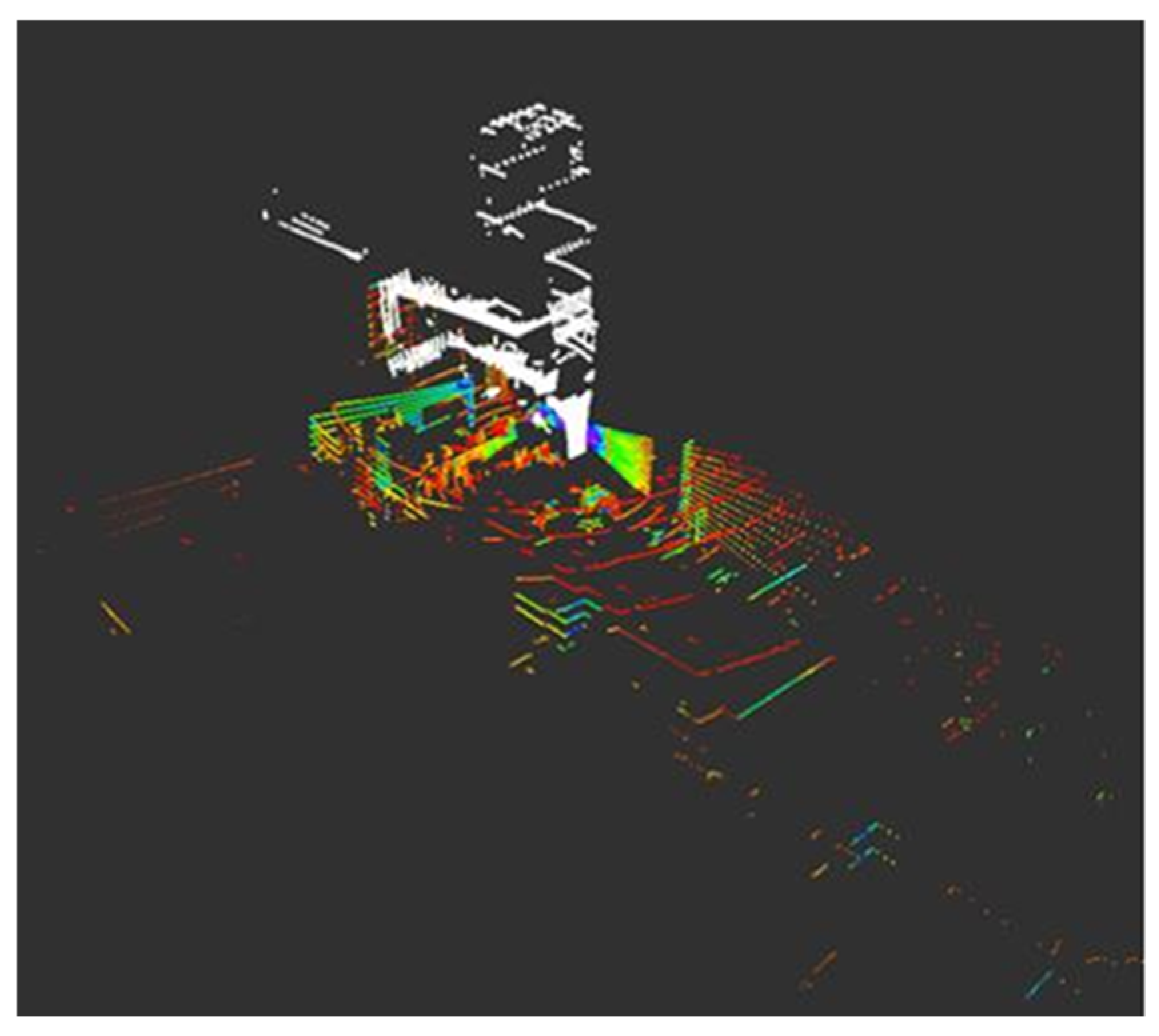
3.5. Color Laser Point Cloud Map Construction

In order to provide more effective road information for inspection robot navigation, this section proposes constructing a color laser point cloud map of the substation by first fusing the image pixel values and the positional information of the laser points to endow them with real color information and then employing the colored laser points to build a color laser point cloud map that is consistent with the color of the environment.

The fusion of a single-frame laser point and the corresponding image pixel is shown in Figure 7, where point P is the next laser point in the camera coordinate system, and laser point P is projected to the image pixel plane by reprojection. The reprojection method is shown in Equation (29):

$$p=\left[\begin{array}{l}u\\ v\\ 1\end{array}\right]={\displaystyle \frac{1}{Z}}\left[\begin{array}{ccc}{f}_x& 0& c_x\\ 0& f_y& c_y\\ 0& 0& 1\end{array}\right]\left[\begin{array}{l}X\\ Y\\ Z\end{array}\right]={\displaystyle \frac{1}{Z}}KP$$

(29)

where $(X,Y,Z)$ are the spatial coordinates of laser point P, matrix K is the internal reference matrix of the camera, which is obtained through the camera calibration, and $p(u,v)$ are the pixel coordinates of the image corresponding to laser point P. If p satisfies $0<=u<=imagewidth$ and $0<=v<=imageheight$, then the laser point is located within the field of view of the camera, and the RGB value of the point can be obtained; if the above conditions are not satisfied, the RGB value cannot be obtained, indicating that the laser point cannot be used for the construction of the color maps.

The RGB pixel value corresponding to laser point P is obtained using Equation (30):

$$P(R,G,B)=f(u,v)$$

(30)

The function $f(u,v)$ indicates the RGB value of the pixel point when the laser point with color is $P(X,Y,Z,R,G,B)$.

A comparison between the stained single-frame laser dots and the image of the environment is shown in Figure 8, from which it can be seen that the color information of the stained laser dots is basically the same as that in the image, and from the laser dots, objects such as walls, tables, people, and calibration boards can be seen.

After fusing the laser points with the corresponding image pixel values in a single frame, the laser points with RGB values are used to build a color laser point cloud map of the surrounding environment. As shown in Figure 9, the laser points acquired by Lidar are in the sensor’s coordinate system, and when building the environment map, the laser points in the sensor’s coordinate system are converted to the global coordinate system by rotating the translation matrix, and they are then accumulated frame by frame to obtain the global color laser point cloud map in the global coordinate system.

The mathematical expression for constructing the color laser point cloud map is shown in Equation (31):

$$P_w=\left[\begin{array}{c}{X}_w\\ Y_w\\ Z_w\end{array}\right]=\left[\begin{array}{ccc}{r}_1(n)& r_2(n)& r_3(n)\\ r_4(n)& r_5(n)& r_6(n)\\ r_7(n)& r_8(n)& r_9(n)\end{array}\right]\ast \left[\begin{array}{c}{X}_s\\ Y_s\\ Z_s\end{array}\right]+\left[\begin{array}{c}{t}_x(n)\\ t_y(n)\\ t_z(n)\end{array}\right]$$

(31)

In the above Equation, $R(n)$ and $t(n)$ are the rotation and translation matrices from the corresponding sensor’s coordinate system (robot’s coordinate system) to the global coordinate system at the current moment, $P(X_s,Y_s,Z_s)$ is the laser point with fused pixel information under the sensor’s coordinate system, and $P_w(X_w,Y_w,Z_w)$ is the laser point with pixel information converted to the global coordinate system. All the laser points are added to the global coordinate system according to Equation (31), and they are then accumulated frame by frame, and finally, a global colored point cloud map of the working environment is constructed. Meanwhile, to ensure the versatility of the algorithm, this algorithm also uses uncolored Lidar data to construct a non-colored laser point cloud map, which is used when the robot works at night or when the colored laser point cloud map is not needed.

4. Experimentation and Analysis

In this section, the proposed VO-Lidar SLAM algorithm for inspection robots described above was experimentally tested through three different environments, namely, indoor scenes, outdoor datasets, and substations, using an substation inspection robot equipped with 3D Lidar and a visual sensor.

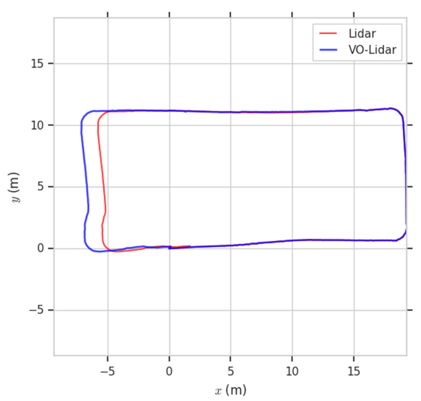
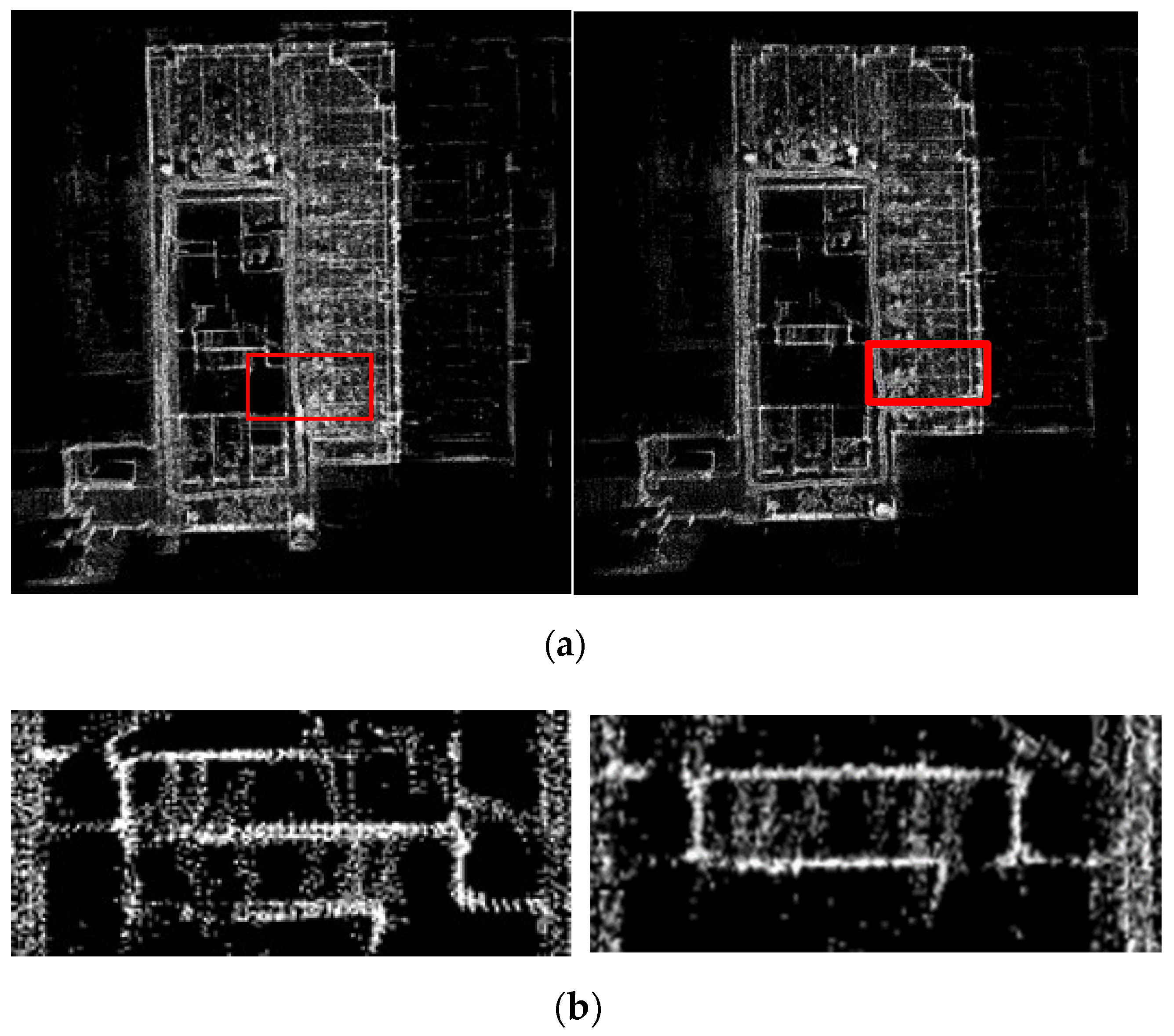
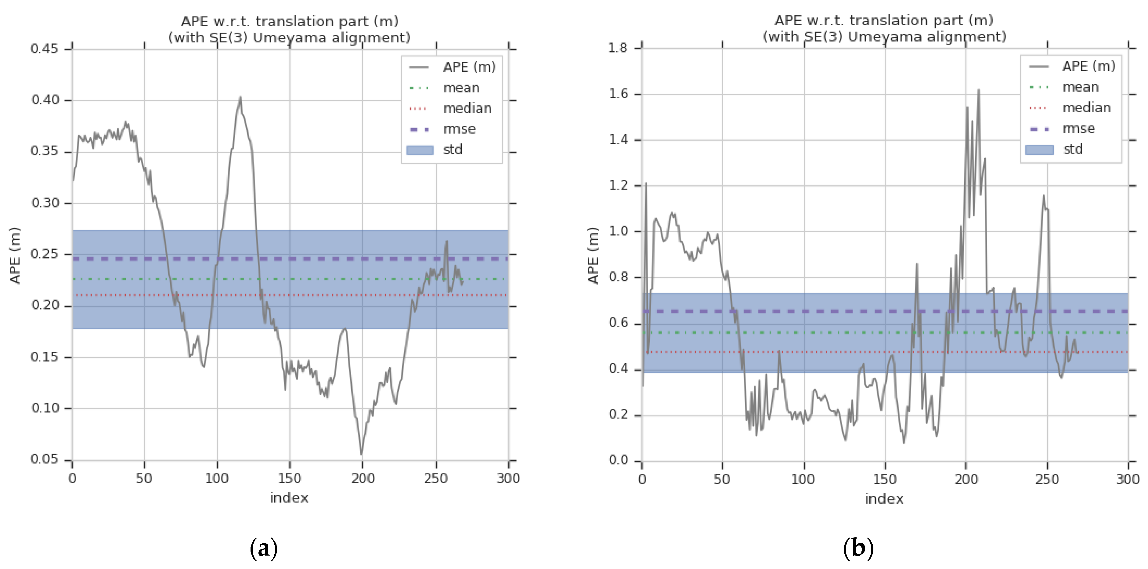
4.1. Indoor Scene Test Results and Analysis

The algorithm underwent its initial testing in a compact indoor setting, specifically a space characterized by a lengthy corridor with uniform environmental contour features. This testing served several purposes: firstly, it was used to ascertain the precision of the VO-Lidar SLAM algorithm; secondly, it was used to scrutinize the influence of the lighting conditions on the algorithm’s localization capabilities by examining trajectory comparisons; and lastly, it was used to evaluate and contrast the impact of color maps against non-color maps within indoor environments. Adopting the loopback error test method in Section 3.4, the inspection robot was set to start from the starting position (0,0), from which it proceeded through the indoor corridor and returned to the starting point again. The deviation in the end position calculated by the algorithm from the start position was regarded as the localization error of the algorithm, and the localization error was calculated according to Equation (24). Figure 10 shows a comparison of the robot’s movement trajectory obtained by the laser SLAM algorithm used in the current inspection robot and the VO-Lidar SLAM algorithm designed in this project with the fusion of the laser and camera; the direction of movement of the inspection robot was in the counterclockwise direction.

Table 2. Comparison of algorithmic localization errors.

Arithmetic	Trajectory Length d(M)	Starting Point Coordinates A (x, y, z)	End Point Coordinates B (x, y, z)	Positioning Error %
Lidar	72.477	(0, 0, 0)	(1.064, 0.199, 0.085)	1.498
VO-Lidar	73.891	(0, 0, 0)	(0.098, 0.128, 0.023)	0.220

shows the coordinates of the end position of the robot motion computed by the two algorithms, Laser SLAM and VO-Lidar SLAM, as well as the localization errors of the two algorithms.

From Table 2, it can be seen that the localization error of the VO-Lidar SLAM algorithm for the inspection robot designed in this paper was much lower than that of the laser SLAM algorithm, which was reduced by 1.278%, and the length of the computed trajectory was also longer than that of the laser SLAM trajectory. The reason is that the inspection robot passed through a long corridor with similar structural features during operation, which caused the laser SLAM algorithm to generate inter-frame matching and localization errors in the environment with similar structural features due to thinking that the robot was at a standstill or in a slow-moving state, whereas the VO-Lidar SLAM algorithm integrates visual position information, and at this time, the laser inter-frame positioning was replaced by the visual position through the position adaptive selection algorithm, reducing the algorithm’s inter-position error by 1.27%, which reduced the localization error of the algorithm. It can also be seen from the trajectories in Figure 10 that the laser SLAM algorithm trajectory traveled less distance than the VO-Lidar SLAM algorithm trajectory, which led to a large error in the computed end position.

The results of the non-stained 3D laser point cloud maps constructed by the laser SLAM algorithm (left) and the VO-Lidar algorithm (right) in an indoor environment are shown in Figure 11. The long corridor with similar structural features in the actual scene was located on the left side of the map, while on the right side of the map was a wide aisle, and the corridor and the aisle were connected in the middle by a passageway, as shown in the location of the red box in the figure. From the left figure, it can be seen that the left and right sides of this connecting channel in the map constructed by laser SLAM were misaligned, and two channels were built, while the connecting channel in the middle of the map constructed by the VO-Lidar algorithm designed in this paper was not misaligned and was consistent with the actual environment. From the comparison of the map construction effects, it can be seen that the environment map constructed by the VO-Lidar SLAM algorithm was better than the original laser SLAM algorithm, which verifies that the laser vision position adaptive selection method can reduce the localization and map construction error of the laser SLAM algorithm in an area of insufficient environmental contour features.

A comparison of the effect of the non-colored laser point cloud map and the colored laser point cloud map in the indoor environment is shown in Figure 12. Figure 12a shows the comparison between the non-colored global laser point cloud map and the colored global laser point cloud map, from which it can be seen that the range of the environment displayed by the colored laser point cloud map was smaller than that of the non-colored laser point cloud map, which was because the scanning range of the Lidar was larger than the range of the field of view of the camera; however, compared with the non-colored map, the colored laser point cloud map could more clearly display the road that required attention for the inspection robot to navigate and avoid obstacles. Since the global map was too large, the map was locally enlarged for comparison, as shown in Figure 12b, and the comparison with the environment image shows that objects such as tables, chairs, floors, walls, columns, doors, etc., in the color laser point cloud map had real color information, which made it easier to distinguish the object categories in the map compared to the non-colored map.

From the indoor environment test results, it can be seen that the VO-Lidar SLAM algorithm designed in this paper is better than the current laser SLAM algorithm used by the inspection robot, both in terms of localization accuracy and map building.

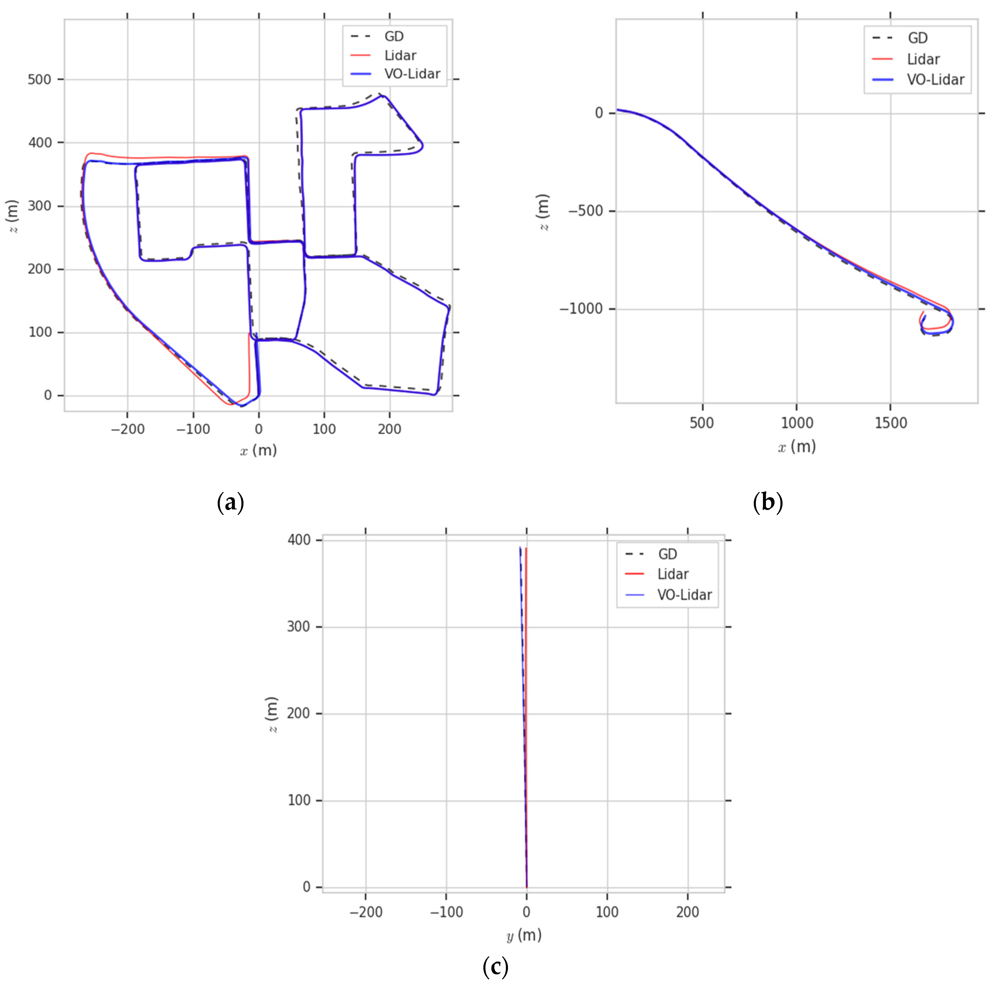
4.2. Outdoor Dataset Test Results and Analysis

In order to more accurately calculate the localization accuracy of the algorithm designed in this paper in various environments, the algorithm’s accuracy was further tested in this section using the KITTI standard dataset. The VO-Lidar SLAM algorithm was tested in KITTI using three large outdoor environment scenes: an urban area, a highway, and a countryside scene. The algorithm’s positioning error was calculated using the comparison tool provided by the KITTI official website, which first took the first frame data position as the starting point of the trajectory, calculated the error between the actual position of the trajectory at 100, 200, and up to 800 m and the baseline position provided by the dataset, and then repeated the above operation with the second frame as the starting point of the trajectory up to the last frame, and it then averaged all the calculated position errors.

The results of the localization errors of the two inspection robot SLAM algorithms in different environments calculated using the KITTI accuracy evaluation tool are shown in

Table 3. Comparison of relative positioning errors of algorithms.

Data Set	Length (m)	Lidar SLAM Relative Positioning Error (%)	VO-Lidar SLAM Relative Positioning Error (%)	Change in Error (%)
Data0 (urban area)	3723	1.37	1.19	$\downarrow$0.18
Data1 (highway)	2451	2.29	1.87	$\downarrow$0.42
Data2 (countryside)	397	1.15	0.85	$\downarrow$0.30

. From the results in the table, it can be seen that in three different outdoor environments, the average length of the moving trajectory of this paper’s algorithm was 2190 m, and the average localization error was 1.30%, which was 0.3% lower than that of the laser SLAM, for which the highway environment’s length was reduced by 0.42%. From the test results, it can be seen that the sensor moving distance had a large impact on the positioning accuracy of the algorithm. The highway was not conducive to feature point extraction and matching due to the long movement distance and the similar and open environment, such that the positioning error was the largest, while the moving distance in the countryside environment was only 397 m, so the positioning error was the lowest.

The inspection robot needs to realize the accurate positioning of each working point. In order to compare the accuracy of the two algorithms in the positioning of the working point, it was necessary to calculate the absolute positioning error of the two algorithms for each point of the trajectory. Here, the rural scene was used to simulate the substation scene, and the absolute positioning error of the two algorithms was analyzed in detail. In this section, the EVO algorithm accuracy evaluation software was used to calculate the absolute positioning error of the two algorithms in the xz plane, in which the RMSE value (root mean square error) of the laser SLAM algorithm’s absolute positioning error was 0.654 m, while the RMSE value of the VO-Lidar SLAM algorithm was 0.245 m, which is a reduction of 0.409 m. The RMSE value of the VO-Lidar SLAM algorithm was 0.245 m, which is a decrease in error. A comparison of the two error curves is shown in Figure 13, from which it can be seen that the maximum and average values of the absolute error of the VO-Lidar SLAM algorithm were lower than those of the laser SLAM algorithm, which shows better qualitative positioning accuracy and stability.

The motion trajectories obtained by the two algorithms in the three different environments are shown in Figure 14. The environments corresponding to (a), (b), and (c) in the figure are the urban area, highway, and countryside, respectively. From the comparison of the trajectory, it can be seen that the VO-Lidar SLAM algorithm’s trajectories (blue) in the urban and rural environments were significantly closer to the baseline trajectories (black dashed lines) than the laser SLAM algorithm’s trajectories (red).

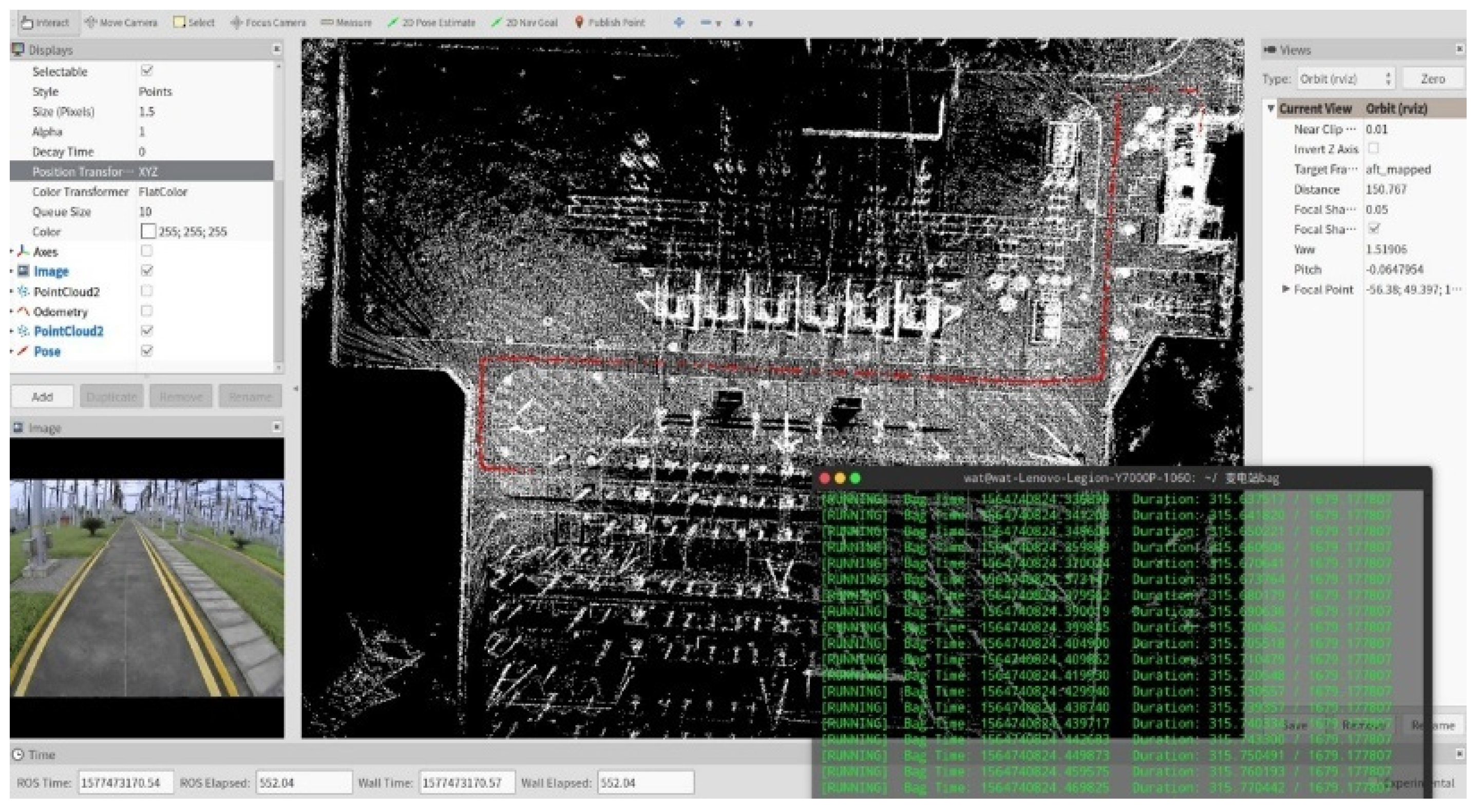
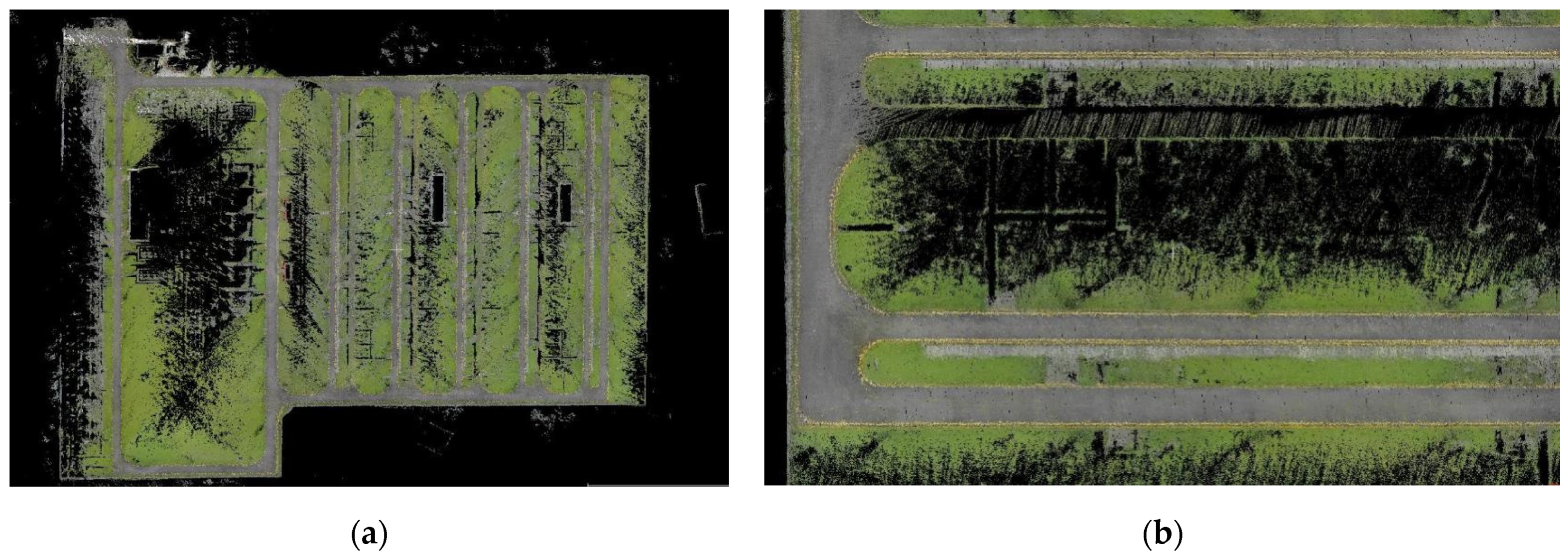
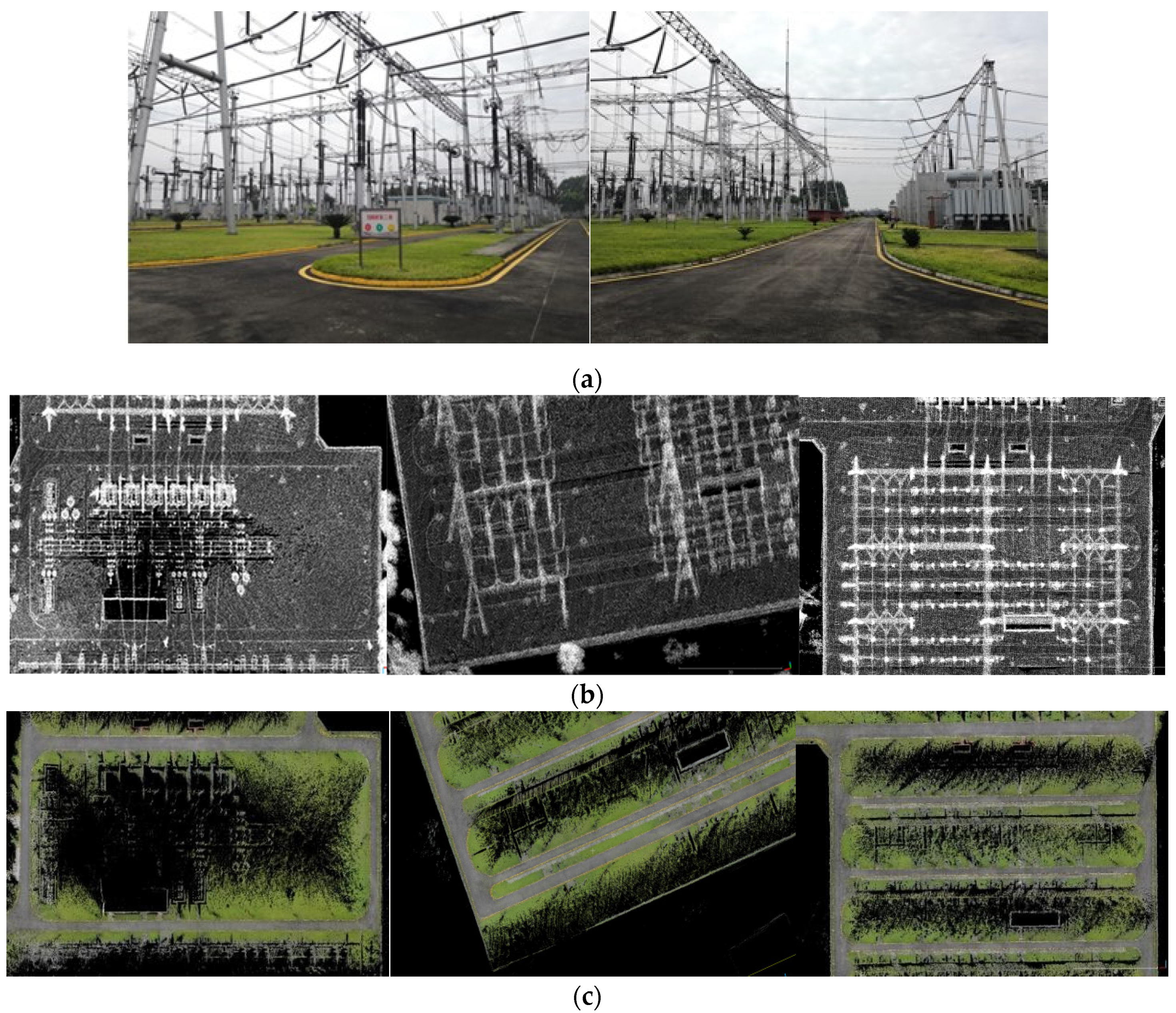
4.3. Substation Scenario Test Results and Analysis

In order to verify the map building effect of the VO-Lidar SLAM algorithm in real scenarios, the algorithm was tested in a real environment of a substation in this section. The test location was a 500 KV substation in Sichuan, and an inspection robot equipped with 3D Lidar and cameras and other sensors was used to move inside the substation to build a map of the substation environment.

The interface of the running process of the VO-Lidar SLAM algorithm is shown in Figure 15. The map in the figure is the non-stained point cloud map constructed by the algorithm up to the current moment, the red line segment is the moving trajectory of the inspection robot estimated by the algorithm, the bottom left corner of the figure is the image of the road environment in front of the inspection robot taken by the camera at the current moment, and the bottom right corner of the figure is the current running time of the algorithm.

The non-colored laser point cloud map constructed by the VO-Lidar SLAM algorithm in the 500 KV substation environment is shown in Figure 16. Figure 16a shows the global non-stained 3D laser point cloud map of the whole substation, where the non-stained laser points are shown in pure white, and it is difficult to see the objects in the global map due to the large area of the substation and the mutual occlusion between the 3D laser points. The transformer part of the global map of the substation was enlarged, as shown in Figure 16b, and the 3D scene information of the transformer and other equipment can be roughly seen from the local map, but it is difficult to distinguish the road situation in this map, which has an impact on the inspection robot’s path planning, autonomous navigation, and other concerns.

The color laser point cloud map constructed by the VO-Lidar SLAM algorithm in the 500 KV substation environment is shown in Figure 17. As can be seen from the figure, the color laser point cloud map clearly shows the road conditions of the inspection route of the inspection robot. The results of enlarging the road environment in the map are shown in (b), in which the gray road surface, the green lawn on both sides of the road, and the yellow boundary line between the road and the lawn are clearly visible.

In order to facilitate the analysis of the two map types constructed by the VO-Lidar algorithm, two different types of local maps corresponding to the same location of the substation were compared with the substation scene image as a reference, as shown in Figure 18. From the substation scene image, it can be seen that there was a height difference between the two sides of the inspection robot caused by the inspection road and the road surface, such that the non-stained laser point cloud map shows the general outline of the road from the structural information, but the description of the road environment is very unclear, and when the road surface was in the same plane as the two sides of the boundary or the height difference was not obvious, the non-stained laser point cloud map could not differentiate between the road boundaries and could not provide the inspection robot navigation with clear road information. From the comparison between the color laser point cloud map and the non-colored laser point cloud map, it can be seen that the color laser point cloud map could clearly describe the road scene that the inspection robot needed to pay attention to for path planning and autonomous navigation, and the road environment color was basically the same as the actual scene color.

5. Conclusions

Aiming at the solving problems of current laser SLAM technology, this paper proposes a SLAM algorithm suitable for substation inspection robots by fusing 3D Lidar information and visual information. The algorithm uses image feature points combined with laser point 3D information to calculate the real position of the image feature points in space, and it restores the scale of monocular visual localization, uses laser positioning and visual positioning with interpolation to correct the point cloud aberration caused by Lidar due to motion, and verifies the aberration correction effect through the localization accuracy testing experiments. For the characteristics of the inter-frame localization error of the laser SLAM algorithm in regions where the environmental structural features are not obvious or are similar, visual localization information is added to the back-end of SLAM, and a position adaptive selection algorithm is designed to replace the laser inter-frame position with the visual position in the above region to improve the robustness of the algorithm. Considering the demand for substation environment maps suitable for inspection robot navigation, this paper integrates the pixel information of the image and the position information of the laser points and constructs color laser point cloud map of the substation, which provides more useful information for inspection robot navigation. As shown through experimental verification, the VO-Lidar SLAM algorithm designed in this paper demonstrated better localization and map building performance than the current laser SLAM algorithm used by inspection robots. Finally, the applicability of the color laser point cloud map of the substation constructed by this algorithm was verified in an actual substation scene.

In future work, this paper considers that multiple cameras could be added to observe environmental images from different angles separately to construct a larger range of color laser point cloud maps. At the same time, the algorithm could be combined with deep learning to construct a semantic map of the substation environment on the basis of the color point cloud map, which would be convenient for inspection robots in terms of recognizing the substation environment scene.

References

1. Pearson, E.; Mirisola, B.; Murphy, C.; Huang, C.; O’Leary, C.; Wong, F.; Meyerson, J.; Bonfim, L.; Zecca, M.; Spina, N.; et al. Robust Autonomous Mobile Manipulation for Substation Inspection. J. Mech. Robot. 2024, 16, 1–17. [Google Scholar] [CrossRef]
2. Wang, D.; Zhang, C.; Li, J.; Zhu, L.; Zhou, B.; Zhou, Q.; Cheng, L.; Shuai, Z. A Novel Interval Power Flow Method Based on Hybrid Box-Ellipsoid Uncertain Sets. IEEE Trans. Power Syst. 2024, 39, 6111–6114. [Google Scholar] [CrossRef]
3. Zhao, S.; Gao, Y.; Wu, T.; Singh, D.; Jiang, R.; Sun, H.; Sarawata, M.; Qiu, Y.; Whittaker, W.; Higgins, I.; et al. SubT-MRS Dataset: Pushing SLAM Towards All-weather Environments. In Proceedings of the IEEE/CVF Conference on Computer Vision and Pattern Recognition, Seattle, WA, USA, 17–21 June 2024; pp. 22647–22657. [Google Scholar]
4. Cai, D.; Li, R.; Hu, Z.; Lu, J.; Li, S.; Zhao, Y. A comprehensive overview of core modules in visual SLAM framework. Neurocomputing 2024, 590, 127760. [Google Scholar] [CrossRef]
5. Zhao, X.; Ren, X.; Li, L.; Wu, J.; Zhao, X. PA-SLAM: Fast and Robust Ground Segmentation and Optimized Loop Detection Laser SLAM System. IEEE Trans. Aerosp. Electron. Syst. 2024, 60, 5812–5822. [Google Scholar] [CrossRef]
6. Zhou, T.; Zhao, C.; Wingren, C.P.; Fei, S.; Habib, A. Forest feature LiDAR SLAM (F2-LSLAM) for backpack systems. ISPRS J. Photogramm. Remote Sens. 2024, 212, 96–121. [Google Scholar] [CrossRef]
7. Wan, Q.; Lv, R.; Xiao, Y.; Li, Z.; Zhu, X.; Wang, Y.; Liu, H.; Zeng, Z. Multi-Target Occlusion Tracking with 3D Spatio-Temporal Context Graph Model. IEEE Sens. J. 2023, 18, 21631–21639. [Google Scholar] [CrossRef]
8. Wan, Q.; Zhu, X.; Xiao, Y.; Yan, J.; Chen, G.; Sun, M. An Improved Non-Parametric Method for Multiple Moving Objects Detection in the Markov Random Field. Comput. Model. Eng. Sci. 2020, 124, 129–149. [Google Scholar] [CrossRef]
9. Ying, Z. Research on Visual SLAM for Sewage Pipe Robot. Master’s Thesis, Southwest Jiaotong University, Chongqing, China, 2018. [Google Scholar]
10. Montemerlo, M.; Thrun, S. Simultaneous localization and mapping with unknown data association using FastSLAM. In Proceedings of the IEEE International Conference on Robotics and Automation, Taipei, China, 14–19 September 2003; Volume 2, pp. 1985–1991. [Google Scholar]
11. Kuang, C.; Chen, W. FastSLAM 2.0: An improved particle filtering algorithm for simultaneous localization and mapping that provably converges. Proc. Int. conf. Artif. Intell. 2003, 133, 1151–1156. [Google Scholar]
12. Zhang, J.; Singh, S. LOAM: Lidar Odometry and Mapping in Real-time. In Proceedings of the Robotics: Science and Systems, Berkeley, CA, USA, 12–16 July 2014; pp. 109–111. [Google Scholar]
13. Zhang, J.; Singh, S. Low-drift and real-time lidar odometry and mapping. Auton. Robot. 2017, 41, 401–416. [Google Scholar] [CrossRef]
14. Hess, W.; Kohler, D.; Rapp, H.; Andor, D. Real-time loop closure in 2D LIDAR SLAM. In Proceedings of the IEEE International Conference on Robotics and Automation, Stockholm, Sweden, 16–21 May 2016; pp. 1271–1278. [Google Scholar]
15. Klein, G.; Murray, D. Parallel tracking and mapping for small AR workspaces. In Proceedings of the IEEE and ACM International Symposium on Mixed and Augmented Reality, Nara, Japan, 13–16 November 2007; pp. 225–234. [Google Scholar]
16. Mur-Artal, R.; Montiel, J.M.M.; Tardos, J.D. ORB-SLAM: A versatile and accurate monocular SLAM system. IEEE Trans. Robot. 2015, 31, 1147–1163. [Google Scholar] [CrossRef]
17. Mur-Artal, R.; Tardós, J.D. Orb-slam2: An open-source slam system for monocular, stereo, and rgb-d cameras. IEEE Trans. Robot. 2017, 33, 1255–1262. [Google Scholar] [CrossRef]
18. Endres, F.; Hess, J.; Sturm, J.; Cremers, D.; Burgard, W. 3-D Mapping With an RGB-D Camera. IEEE Trans. Robot. 2013, 30, 177–187. [Google Scholar] [CrossRef]
19. Henry, P.; Krainin, M.; Herbst, E.; Ren, X.; Fox, D. RGB-D Mapping: Using Depth Cameras for Dense 3D Modeling of Indoor Environments. In Experimental Robotics, Springer Tracts in Advanced Robotics; Springer: Berlin/Heidelberg, Germany, 2014; Volume 79, pp. 477–491. [Google Scholar]
20. Newcombe, R.A.; Izadi, S.; Hilliges, O.; Molyneaux, D.; Kim, D.; Davison, A.J.; Kohi, P.; Shotton, J.; Hodges, S.; Fitzgibbon, A. KinectFusion: Real-time dense surface mapping and tracking. In Proceedings of the IEEE International Symposium on Mixed and Augmented Reality, Basel, Switzerland, 26–29 October 2011; pp. 127–136. [Google Scholar]
21. Engel, J.; Stückler, J.; Cremers, D. Large-scale direct SLAM with stereo cameras. In Proceedings of the IEEE/RSJ International Conference on Intelligent Robots and Systems, Hamburg, Germany, 28 September–2 October 2015; pp. 1935–1942. [Google Scholar]
22. Li, J.; Zheng, K.; Gao, L.; Ni, L.; Huang, M.; Chanussot, J. Model-informed Multi-stage Unsupervised Network for Hyperspectral Image Super-resolution. IEEE Trans. Geosci. Remote Sens. 2024, 62, 5516117. [Google Scholar] [CrossRef]
23. Li, J.; Zheng, K.; Li, Z.; Gao, L.; Jia, X. X-shaped interactive autoencoders with cross-modality mutual learning for unsupervised hyperspectral image super-resolution. IEEE Trans. Geosci. Remote Sens. 2023, 61, 5518317. [Google Scholar] [CrossRef]
24. Zhang, J.; Kaess, M.; Singh, S. Real-time depth enhanced monocular odometry. In Proceedings of the IEEE/RSJ International Conference on Intelligent Robots and Systems, Chicago, IL, USA, 14–18 September 2014; pp. 4973–4980. [Google Scholar]
25. Gao, X. Fourteen Lectures on Vision SLAM: From Theory to Practice; Electronic Industry Press: Beijing, China, 2017. [Google Scholar]
26. Arun, K.S.; Huang, T.S.; Blostein, S.D. Least-squares fitting of two 3-D point sets. IEEE Trans. Pattern Anal. Mach. Intell. 1987, 5, 698–700. [Google Scholar] [CrossRef] [PubMed]
27. Pomerleau, F.; Colas, F.; Siegwart, R. A review of point cloud registration algorithms for mobile robotics. Found. Trends Robot. 2015, 4, 1–104. [Google Scholar] [CrossRef]
Figure 1. Overall framework of the SLAM algorithm for 3D Lidar and vision fusion for use by inspection robots.
Energies 18 02797 g001
Figure 2. VO-Lidar SLAM algorithm framework.
Energies 18 02797 g002
Figure 3. Before and after laser point cloud conversion.
Energies 18 02797 g003
Figure 4. Schematic diagram of the laser projection method.
Energies 18 02797 g004
Figure 5. Schematic diagram of point cloud distortion correction.
Energies 18 02797 g005
Figure 6. Laser and vision position adaptive selection method.
Energies 18 02797 g006
Figure 7. Laser point and pixel value fusion method.
Energies 18 02797 g007
Figure 8. Schematic diagram of single-frame laser spot coloring effect: (a) real images of the environment; (b) image of the environment after single-frame laser point staining.
Energies 18 02797 g008
Figure 9. Sensor coordinate system: global coordinate system.
Energies 18 02797 g009
Figure 10. Comparison of algorithmic trajectories for indoor scenes.
Energies 18 02797 g010
Figure 11. Comparison of map building results of indoor scene algorithms: (a) global map comparison; (b) local map comparison.
Energies 18 02797 g011
Figure 12. Comparison of point cloud map effect before and after coloring: (a) global map comparison; (b) local map comparison.
Energies 18 02797 g012
Figure 13. Algorithm absolute positioning error curve: (a) laser SLAM absolute error profile; (b) VO-Lidar SLAM absolute error profile.
Energies 18 02797 g013
Figure 14. Comparison of algorithmic trajectories for dataset scenarios: (a) urban area; (b) highway; (c) countryside.
Energies 18 02797 g014
Figure 15. VO-Lidar SLAM runtime interface.
Energies 18 02797 g015
Figure 16. Non-stained laser point cloud map of the substation: (a) substation global non-colored maps; (b) substation localized non-colored maps.
Energies 18 02797 g016
Figure 17. Color laser point cloud map of the substation: (a) global color point cloud map of substations; (b) localized color point cloud map of the substation.
Energies 18 02797 g017
Figure 18. Comparison of the effects of the two map types: (a) substation scene images; (b) non-stained laser point cloud map of substations; (c) color laser point cloud maps of substations.
Energies 18 02797 g018