Quasi-Static Tractor Implement Model for Assessing Energy Savings in Partial Electrification

Abstract

This paper presents a quasi-static model for assessing potential energy savings through partial electrification of a land leveler implement. The quasi-static model simulates the behavior of the hydraulic circuit components, including the pump and a spool-type flow divider, for a commercial land leveler used in agricultural applications. Two electrification schemes are presented. In the first scheme, the pump, originally driven at fixed speed by the PTO, is driven at variable speed by an electric drive, with no changes in the hydraulic circuit. In the second electrification scheme, the decentralization of the hydraulic system is implemented by using separate variable-speed pumps for each actuator. Results show significant potential energy savings of 9–22% with the first electrification scheme and 45–53% with the second scheme, compared to the traditional non-electrified setup. Our findings demonstrate that electrification could be a strategic choice to improve the efficiency of tractor implements and agricultural machinery.

1. Introduction

Among the great global challenges, the greenhouse effect and global warming certainly represent one of the greatest threats for present and future generations. Politics and industry are working together to reduce emissions in many industrial applications, and the technical regulations are becoming increasingly stringent and ambitious. The agricultural sector is also addressing the environmental issue, with much research underway on the electrification of tractors and agricultural machinery [1,2,3,4]. Converting tractors to electric power presents significant challenges, owing to their complex systems and high energy consumption needs. The state of the art for the traction of NRMM and agricultural machinery is the diesel engine, but recently, fully electric off-road vehicles, equipped with battery or fuel cells and driven by electric motors, have been investigated and developed [5,6,7]. There also exist several examples of hybrid (diesel–electric) powertrain designs [8,9,10,11].

In the case of tractors, the prime mover also delivers power to the connected tools through the power take off (PTO). There are four possible types of connection between the tractor and the implements, outlined as follows [12]: mechanical connection via the PTO shaft, hydraulic connection via fluid power, pneumatic connection via pressurized air, and electrical connection via a high- or low-power interface. Matching three powertrain topologies (diesel, hybrid, and electric) with four implement types (mechanical, hydraulic, pneumatic, and electric) leads to a significant number of combinations.

Each combination offers its own advantages and disadvantages in terms of economical costs and savings, fuel efficiency, emissions, and practicality [13]. It is expected that agriculture will become increasingly more autonomous [14,15,16] and focused on precision farming in the future [17,18,19]. Electrified implements will play a key role in the near future in the agricultural sector because they combine very well with automatic and digital processes [20,21,22,23]. Moreover, electrified implements prove to be more energy efficient than the traditional non-electric models. Several tractor and implement manufacturers studied and built different electrified implements in the last 20 years, investigating and proving the improvements in efficiency and fuel consumption [24,25,26,27,28,29,30,31]. All these works highlight the interest of electrification in both industry and research sectors. Very often, the complete electrification of the implement, i.e., a complete substitution of hydraulic actuators, is not feasible or possible due to the space constraints or technological capability. Therefore, partial electrification has to be considered in order to increase the implement efficiency, exploiting the additional degrees of freedom that electrification allows during operation. In partially electrified implements, an electric motor is used to drive the implement instead of the mechanical PTO, but the implement keeps its hydraulic circuit. By implementing partial electrification, manufacturers and farmers can benefit from the electric technology enhancing the conventional hydraulic circuits, which are still effective for high-force applications common in agricultural implements.

Load sensing, introduced in agricultural machinery in 1974 [32], is a hydraulic system technology that adjusts the pump output to match the exact flow and pressure demands of the system plus a given margin, improving efficiency in machinery and equipment. Nowadays, load sensing systems are the state of the art in agricultural machinery, but they no longer offer the most efficient solution. In fact, load sensing is usually adopted with a fixed-speed pump, which is not really efficient in cases of fast-changing loads and at no load or partial load. Adopting variable-speed operation for the pump would instead allow, thanks to proper control, noticeable energy savings.

In this paper, a land leveler is modeled and analyzed to assess potential energy savings through partial electrification. A quasi-static model, which effectively simulates the hydraulic circuit of the implement is proposed, enabling the assessment of the power consumption in the traditional configuration (fixed-speed pump) and in the case of electrification (variable-speed pump). This paper is structured as follows: Section 2 presents and describes the land leveler, the experimental tests, the quasi-static model, and the proposed electrification schemes; Section 3 reports the simulation results, while a discussion is provided in Section 4; and Section 5 summarizes the conclusions.

2. Methodology

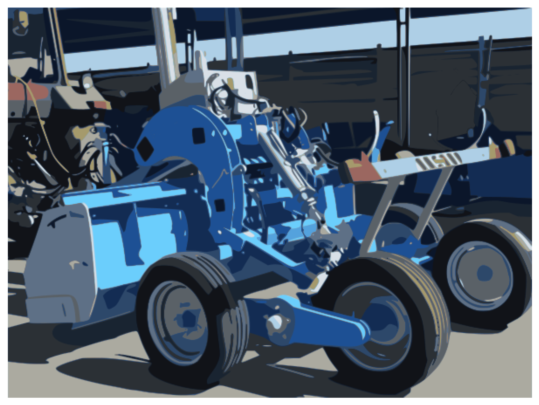
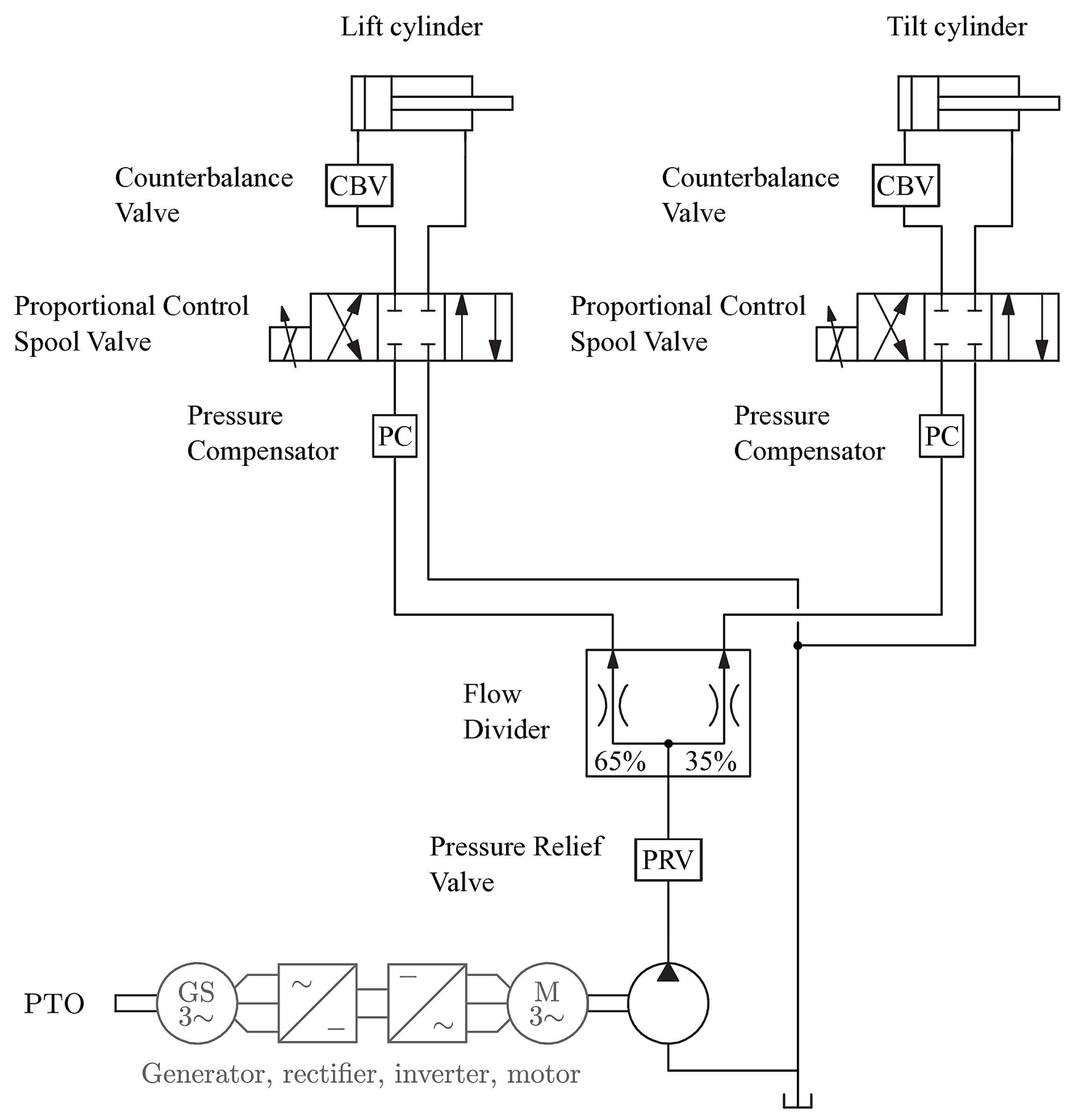
2.1. Tractor Implement Under Study

A land leveler is an agricultural implement used to smooth and level the surface of a field. By eliminating high spots and filling in low areas, this implement can improve water management, reduce soil erosion, and enhance overall crop growth. The land leveler is typically attached to the tractor’s rear and it is dragged during operation. Land levelers available on the market can vary greatly in size. Basic land levelers feature a lift cylinder for height adjustment, controlled by laser guidance. More advanced land levelers also feature a tilt cylinder and a GPS guidance to improve leveling precision throughout the field. Land levelers can be used in both agricultural fields and sports fields.

Figure 1 shows the land leveler studied in this paper. It is a laser-controlled leveler machine with a lift and tilt cylinder. It is a commercial product to which measurement sensors have been added to conduct experimental tests. The scheme of the hydraulic circuit of the implement is shown in Figure 2. A fixed displacement pump (10.8 cm³/rev) provides flow to the hydraulic circuit consisting of two actuators. Both the lift and tilt cylinders are double-acting cylinders. The cap and annular areas of the lift cylinder are 55.31 cm² and 38.44 cm², while the cap and annular areas of the tilt cylinder are 33.72 cm² and 27.81 cm². A Counterbalance Valve (CBV) is connected to each cylinder to allow for proper control with overrunning loads. Both CBVs have a pilot ratio of 4.25, a spring pressure stiffness of 100 MPa/m, and a max opening of 1 mm. The CBV connected to the lift cylinder has a pressure setting of 210 bar, while the CBV connected to the lift cylinder has a pressure setting of 350 bar. The cylinders are controlled by proportional directional control spool valves. Pressure compensators (PCs) are used to maintain a constant pressure drop across the proportional control valves, regardless of the load pressure. The load sensing system adjusts the supply pressure to match the highest load pressure in the system, plus a margin that is calibrated to 12 bar in this application. The pump flow is divided on the lift and tilt cylinders by a flow divider with a ratio of 60:40. The pump operates at a fixed speed of 2052 rpm, driven by the PTO (540 rpm) through a gearbox with a ratio of 1:3.8. Finally, the pressure relief valve (PRV) is set to a pressure of 180 bar.

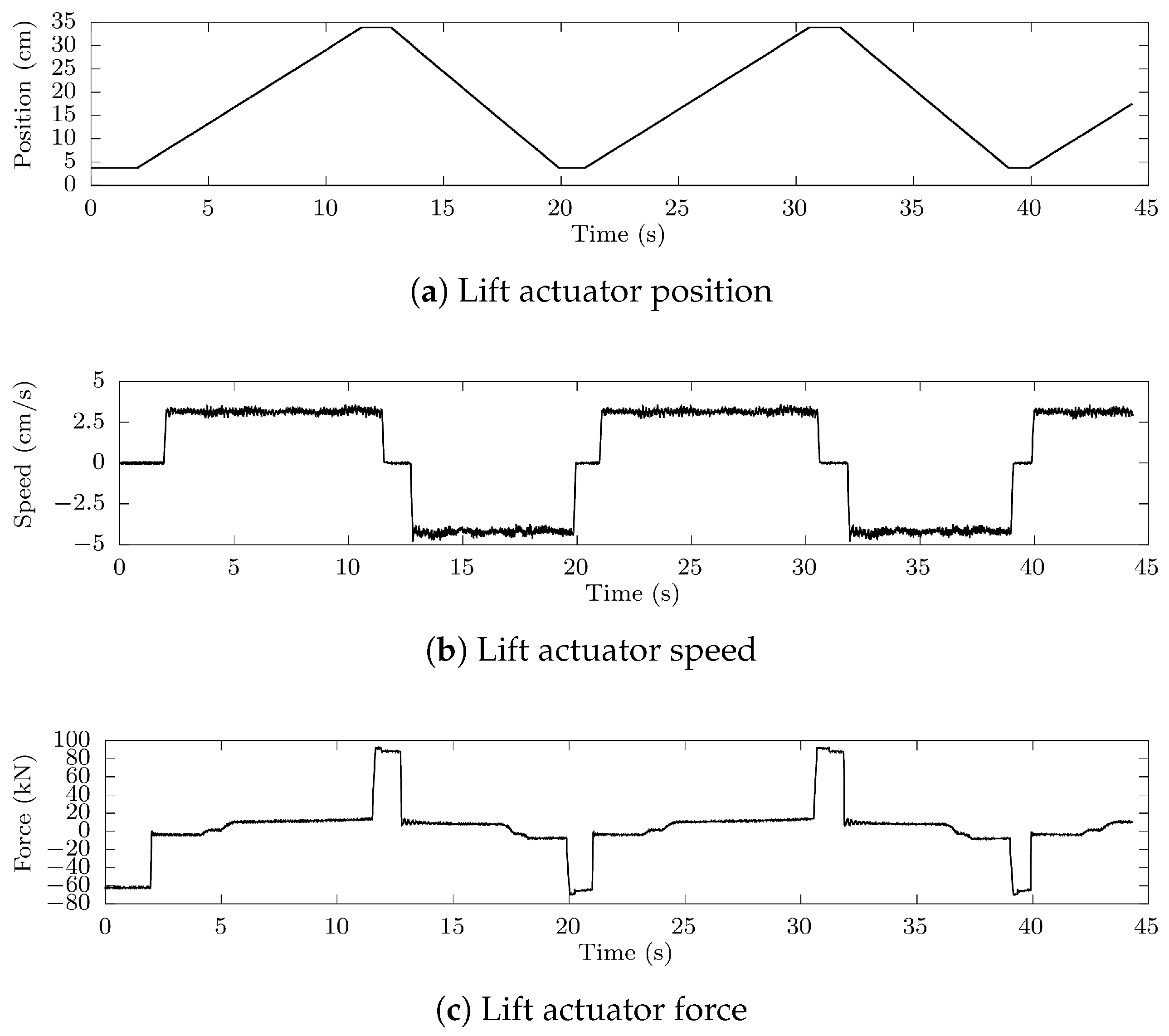
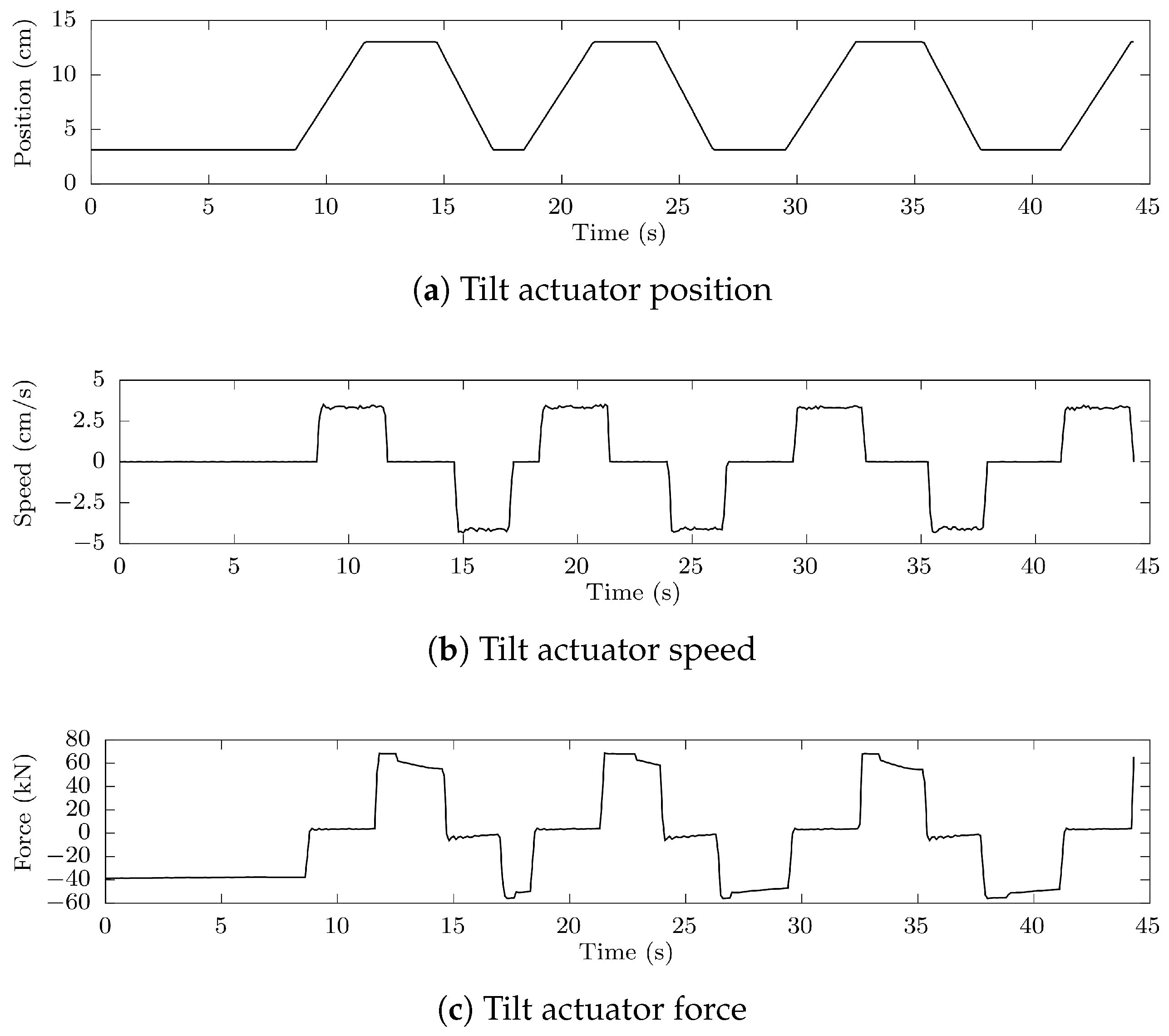
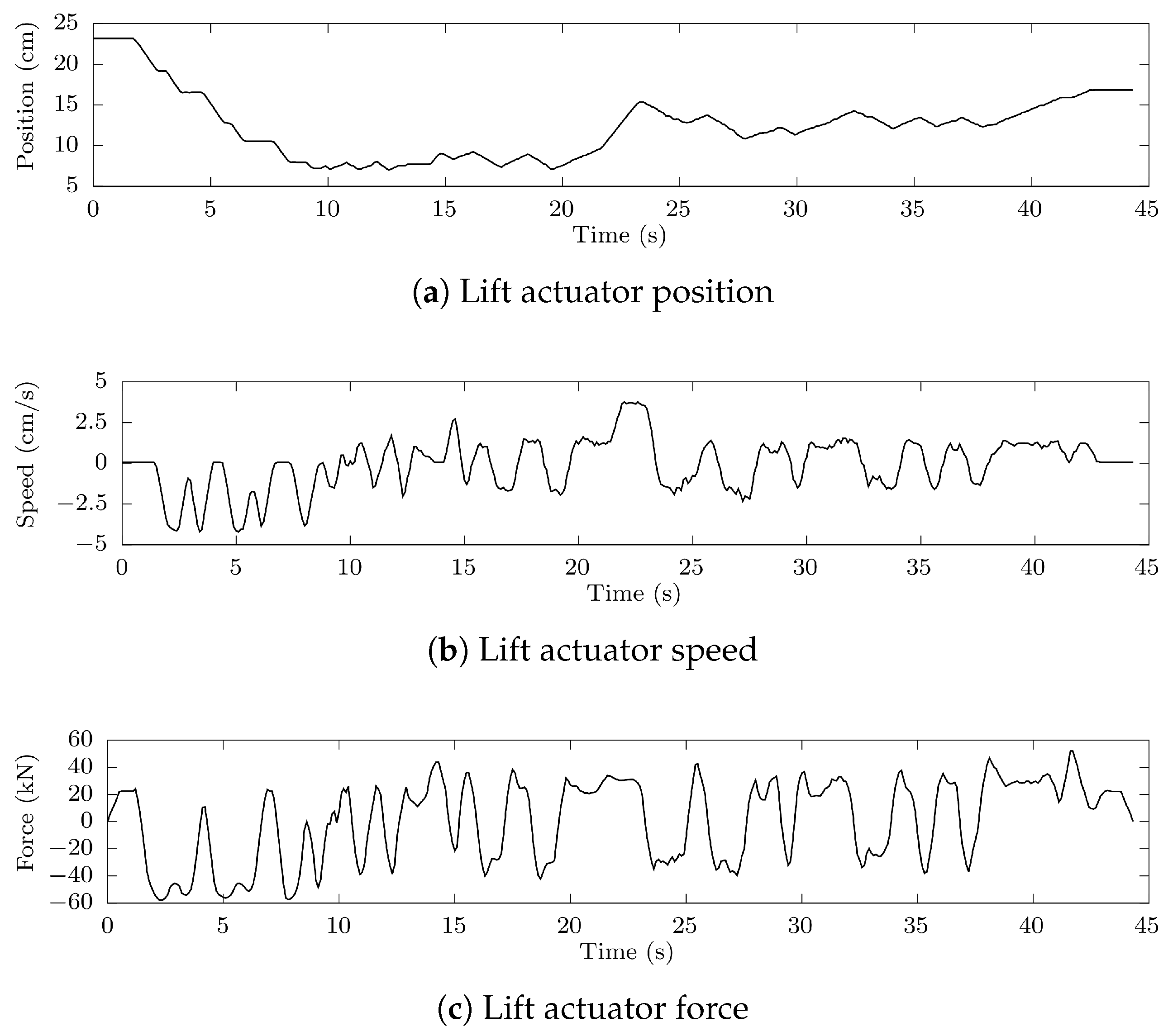
2.2. Experimental Tests Performed on the Implement

The land leveler under study is a commercial implement to which the following measurement sensors have been added: torque and speed sensors at the PTO, and hydraulic pressure and position sensors at the cylinders. Specifically, the torque and speed sensors measure the PTO torque and speed in Nm and rpm, respectively. The hydraulic pressure sensors, installed on both the cap and annulus sides of the lift and tilt cylinders, measure the hydraulic pressure in bar. With the cap and annulus areas of cylinders being known, the fluid force exerted on the piston can be calculated by applying (5). The force is expressed in kN. Finally, the position sensors installed on the cylinders measure the position and speed, in cm and cm/s, respectively, of the lift and tilt pistons during extension and retraction.

Experimental tests have been performed on the implement, both indoor and outdoor. In all tests, the implement was connected to the tractor with the PTO operating at a fixed speed. During the tests, the operator commanded a series of openings and closings of the hydraulic valves using the controllers.

Figure 3 and Figure 4 show the results of the indoor tests for the lift and tilt actuators, respectively. In the indoor tests, the tractor and the land leveler were in a fixed position with the engine running. In fact, the actuators operated at no load during the indoor tests.

The first data log, shown in Figure 3, relates to the lift cylinder. During the 44.3 s test, the actuator extends and retracts twice at maximum flow rate. The lift actuator’s motion is in the range from 3.8 to 33.9 cm, with extension and retraction speeds of 3.2 cm/s and −4.2 cm/s, respectively. The measured force ranges from −69.4 to 92 kN.

The second data log, related to the tilt cylinder, is presented in Figure 4. Over the same duration, it extends four times and retracts three times at maximum flow rate. Its motion ranges from 3 to 13 cm, with an extension speed of 3.95 cm/s and a retraction speed of −4.8 cm/s. The measured force ranges from −56.8 to 71 kN.

The third data log, related to the lift cylinder, is shown in Figure 5. The data were collected during a field test, with the land leveler being dragged by the tractor and the height of the implement being adjusted by the lift actuator action. The duration of the log is 44.3 s. The lift actuator position varies from 7 to 23 cm during the test, with the speed ranging from −4.3 to 4 cm/s. The minimum value of the measured actuator force is −58 kN, while the maximum is 54.4 kN.

2.3. Quasi-Static Model of the Hydraulic Circuit

The hydraulic circuit of the considered land leveler, based on load sensing, has been modeled through a quasi-static model implemented on Simulink. The quasi-static model developed in this paper is based on the model presented in [33], with a major update consisting of the implementation of the flow divider and the simultaneous operation of two actuators. Quasi-static models have the advantage of requiring few parameters to simulate a hydraulic system, with the drawback of not being highly accurate in all simulation conditions. Nevertheless, the dynamic inaccuracies are almost negligible when the focus of the simulation is the energy assessment of the system and the approach demonstrates good accuracy, which is also in agreement with experimental tests. The following assumptions were made in the model:

• Each valve’s metering orifice is modeled as a turbulent flow orifice, as commonly carried out in the literature [34].
• Identical parameters ($C_d$ and $A\left(x\right)$ in (1)) are used for both the flow paths of the control valve during extension (P-A and B-T) and retraction (P-B and A-T).
• Pressure drop through check valves is negligible when flow is permitted.
• Leakage, mechanical friction, and compressibility effects are considered negligible.
• Tank pressure is assumed to be zero.
• Actuator force and speed are known.
• A constant pressure drop is maintained across the inlet orifice (load sensing): during extension—$p_s$−$p_A$ = $\Delta p_{LS}$; during retraction—$p_s$−$p_B$ = $\Delta p_{LS}$, where $\Delta p_{LS}$ is the desired pressure margin, kept constant to ensure a unique correlation between valve spool displacement and flow rate.
• No regeneration occurs; all fluid leaving the cylinder goes to the tank.
• No energy recovery is considered.

Consistently with the assumptions made for the quasi-static model, each actuator in the hydraulic circuit can be represented with the scheme in Figure 6, where the CBV is used to allow for a proper control with overrunning loads. The equations underlying the quasi-static model are described below. The turbulent flow through an orifice can be expressed by the following orifice equation [34]:

$$Q=C_D·A\left(x\right)·\sqrt{{\displaystyle \frac{2\Delta p}{\rho }}}$$

(1)

where Q is the flow rate in L/min, $C_D$ is the flow discharge coefficient (adimensional), $A\left(x\right)$ is the orifice passage area in mm², x is the spool displacement in m, $\rho$ is the fluid density in kg/m³, and $\Delta p$ is the pressure drop across the orifice in bar. Applying the orifice equation to the flow paths of the control valve, the following holds:

$$Q_{PA}=C_D·A\left(x\right)·\sqrt{{\displaystyle \frac{2\Delta p_{PA}}{\rho }}}$$

(2)

$$Q_{BT}=C_D·A\left(x\right)·\sqrt{{\displaystyle \frac{2\Delta p_{BT}}{\rho }}}$$

(3)

With the introduced hypotheses on $C_D$ and $A\left(x\right)$, the pressure drops across the two flow paths of the proportional control valve ($\Delta p_{BT}$ and $\Delta p_{PA}$) are proportional to the square of the respective flow rate as follows:

$${\displaystyle \frac{\Delta p_{BT}}{\Delta p_{PA}}}={\left({\displaystyle \frac{Q_{BT}}{Q_{PA}}}\right)}^2$$

(4)

The fluid exerts a force, denoted as F, on the piston. This force in N can be expressed mathematically using the following equation:

$$F=p_1{A}_1-p_2{A}_2$$

(5)

where $A_1$ and $A_2$ are the cap and annulus area in m², respectively. Thus, the pressure $p_1$ at the cylinder chamber $A_1$ (cap) expressed in pascal (Pa) can be be obtained as follows:

$$p_1={\displaystyle \frac{F+p_2·A_2}{A_1}}$$

(6)

and, knowing the pressure margin $\Delta p_{LS}$ in Pa introduced by the load sensing system, it turns out that the supply pressure (downstream of the flow divider) can be computed as follows:

$$p_s=p_1+\Delta p_{LS}$$

(7)

or equivalently, as follows:

$$p_s={\displaystyle \frac{F+p_2·A_2}{A_1}}+\Delta p_{LS}$$

(8)

where the pascal-to-bar conversion is given by 1 bar = 10⁵ Pa. Equation (8) can be used to evaluate the pressure required at the pump based on the load demand. In particular, (8) is valid during cylinder extension, since CBV is not acting. Conversely, during cylinder retraction, the CBV action needs to be taken into account and (8) is not valid and needs to be adjusted. The force balance of the CBVs during retraction can be expressed by the following:

$$F_0+c·x_{CBV}=p_1·A_{pilot}+p_2·A_{load}-p_B·A_{back}$$

(9)

where $A_{pilot}$, $A_{load}$, and $A_{back}$ are the effective areas of the spool that create a force when a pressure is applied in m², $F_0$ is the spring setting in N, c is the spring rate in N/m, and $x_{CBV}$ is the CBV spool displacement in m. The pressure drop through the CBV during retraction is as follows:

$$p_1-p_A={\displaystyle \frac{\rho }{2}}{\left({\displaystyle \frac{Q_B}{C_D·A\left(x_{CBV}\right)}}\right)}^2$$

(10)

where the orifice passage area is assumed to be proportional to the CBV spool displacement $x_{CBV}$ ($A=b·x_{CBV}$, with b being a constant).

A cubic equation of the spool displacement $x_{CBV}$, omitted here, can be obtained combining Equations (5), (9) and (10), and $p_s-p_B=\Delta p_{LS}$. By solving the equation, $x_{CBV}$, and consequently $p_s$, can be computed. Regarding the flow rate, for linear actuators, it is computed multiplying the speed by the piston area at the inlet side ($A_1$ during extension and $A_2$ during retraction). The block diagram of the quasi-static model for a single cylinder is depicted in Figure 7. Given the data logs of actuator force and speed as input, the model computes and delivers the pump pressure and flow rate as output. The model needs to be properly calibrated as follows: the cap and annular areas of the cylinder ($A_1$ and $A_2$), CBV pilot ratio, CBV spring rate, CBV pressure setting, and $\Delta p_{LS}$ are required as model parameters. The accurate tuning of the model parameters can be performed comparing the simulation results with the experimental measurements.

Figure 8 evaluates the accuracy of the quasi-static model for the considered implement, using the lift cylinder as an example. The first data log (indoor test—Figure 3) was used for comparison. The simulated pressures $p_1$ and $p_2$ (outputs of the quasi-static model in Figure 7) are compared with the hydraulic pressures $p_1$ and $p_2$, which were previously measured on the cylinder with the pressure sensor. Some deviations can be observed at the beginning and end of the cylinder extension and retraction. However, overall, there is a very good match between experimental data logs and simulation results, confirming that the quasi static model is reliable and accurate both in extension and retraction operations. The same quasi-static model has also proven to be suitable in another application—the modeling of the hydraulic circuit of a mobile crane [33].

The extended quasi-static model, which will be explained in the next subsection, facilitates the computation of the pressure and flow rate for both the lift and tilt actuators simultaneously ($p_{s\_\mathrm{lift}}$ and $Q_{\mathrm{lift}}$ and $p_{s\_\mathrm{tilt}}$ and $Q_{\mathrm{tilt}}$, respectively).

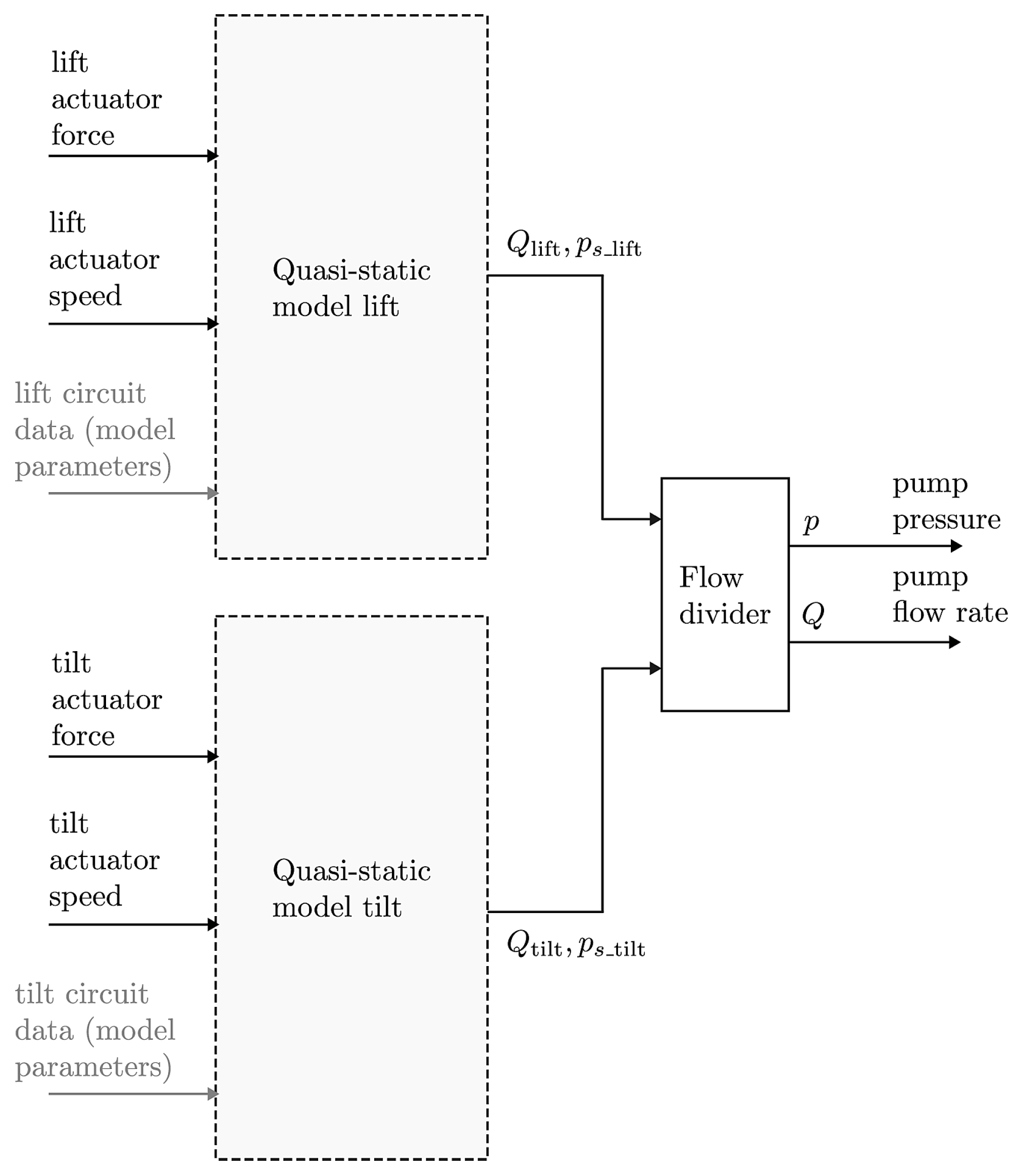
2.4. Extension of the Quasi-Static Model for Two Cylinders

A major update introduced in this paper with respect to the quasi-static model in [33] is the implementation of the flow divider. The flow divider is a device that divides a single input flow into multiple output flows, often in predetermined ratios. For the considered hydraulic circuit, as shown in Figure 2, the flow divider divides the pump flow in lift and tilt flows with a ratio of 60:40. Consistent with the design rules, the pump displacement has been chosen to satisfy the flow rate requirements of this application. The flow divider can be modeled with two fixed orifices and an infinite position 4/3 spool valve, as shown in Figure 9a. The spool position is determined by the two pressures downstream of the two orifices ($p_{s\_\mathrm{lift}}$ and $p_{s\_\mathrm{tilt}}$ in Figure 9b). Depending on the pressures downstream of the two orifices, the lighter load gets compensated by the movement of the spool valve that applies a restriction to the least loaded branch [34]. The pressure drop curve for the considered flow divider is shown in Figure 9c, and it is implemented as a lookup table in the quasi-static model. This curve applies when both lift and tilt loads are identical, specifically when $p_{s\_\mathrm{lift}}=p_{s\_\mathrm{tilt}}$. In this scenario, the spool remains in its neutral position, enabling unrestricted flow through both pathways at an equal 50:50 ratio. When $p_{s\_\mathrm{lift}}>p_{s\_\mathrm{tilt}}$, the load on the lift cylinder is higher than the load on the tilt cylinder, and the flow divider applies a restriction on the tilt branch. In this scenario, the pressure drop through the flow divider $\Delta p_{FD}$ can be computed as the pressure drop on the most loaded branch (the lift branch), which corresponds to multiplying the output of the lookup table for the scaling factor ${\left({\displaystyle \frac{0.60}{0.5}}\right)}^2$. In the other scenario, $p_{s\_\mathrm{tilt}}>p_{s\_\mathrm{lift}}$, the flow divider applies a restriction on the lift branch, and the pressure drop $\Delta p_{FD}$ can be computed on the tilt branch by multiplying the output of the lookup table for the scaling factor ${\left({\displaystyle \frac{0.40}{0.5}}\right)}^2$. In all scenarios, when we know the pressure drop across the flow divider, the pump pressure p can be computed as the sum of $\Delta p_{FD}$ with the highest $p_{s\_\mathrm{lift}}$ and $p_{s\_\mathrm{tilt}}$.

Finally, the pump hydraulic power in watt (W) can be assessed as follows:

$$P=p·Q$$

(11)

The pump flow rate Q is constant and equal to 22.1 L/min during fixed-speed operation. The calculation is performed by taking into account that the pump has a displacement of 10.8 cm³/rev and runs at a speed of 2052 rpm (that is, the PTO speed of 540 rpm increased by the 1:3.8 gearbox ratio). In the case of variable-speed operation, the pump flow rate Q can be easily evaluated in the quasi-static model by taking the max of $Q_{\mathrm{lift}}$ and $Q_{\mathrm{tilt}}$ scaled by the flow divider ratio. The block diagram of the proposed quasi-static model is depicted in Figure 10.

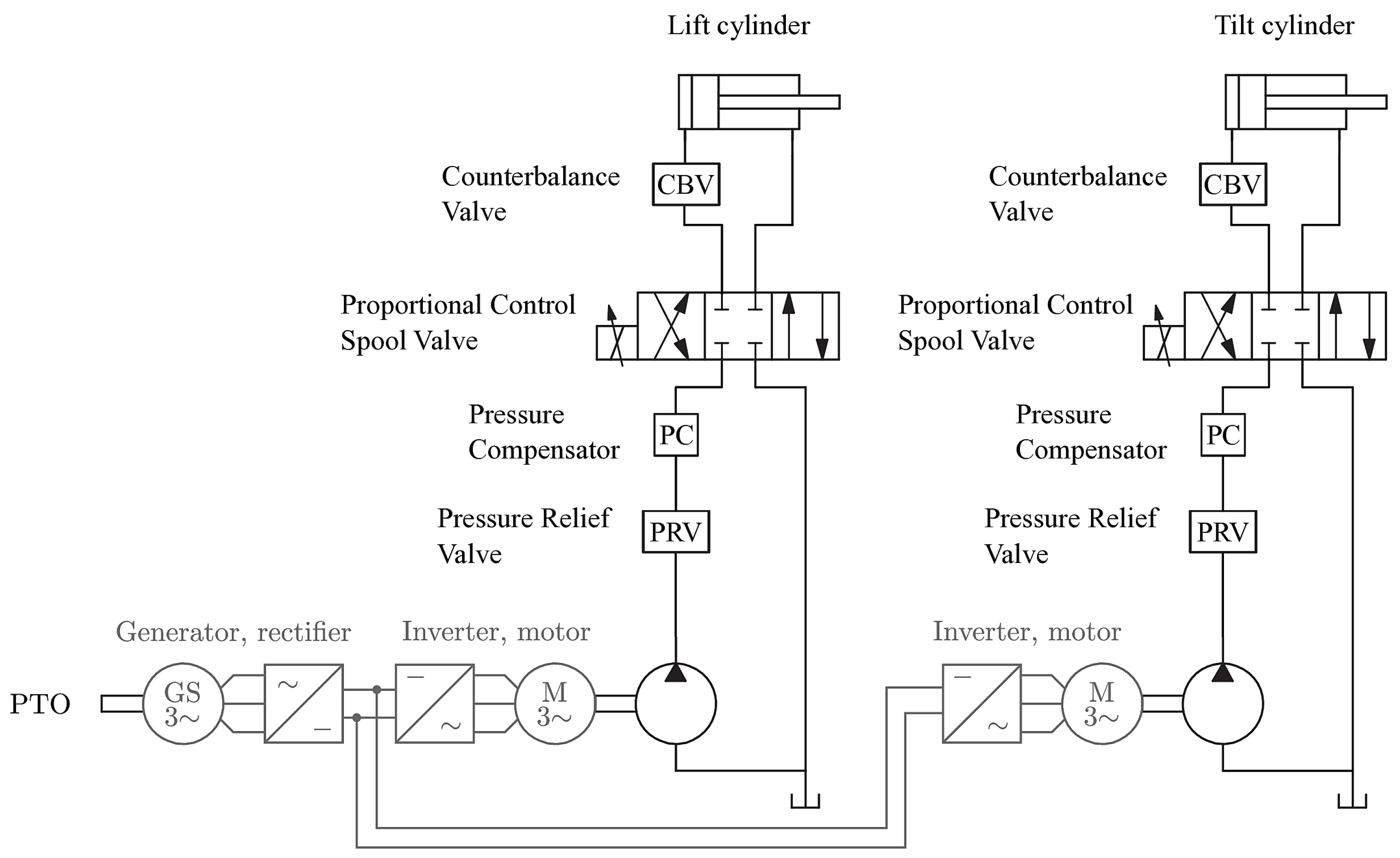
2.5. Proposed Electrification Schemes

The quasi-static model developed and proposed in this article will be simulated in three configurations, as follows:

• At fixed speed.
• At variable speed (first electrification scheme).
• At variable speed (second electrification scheme).

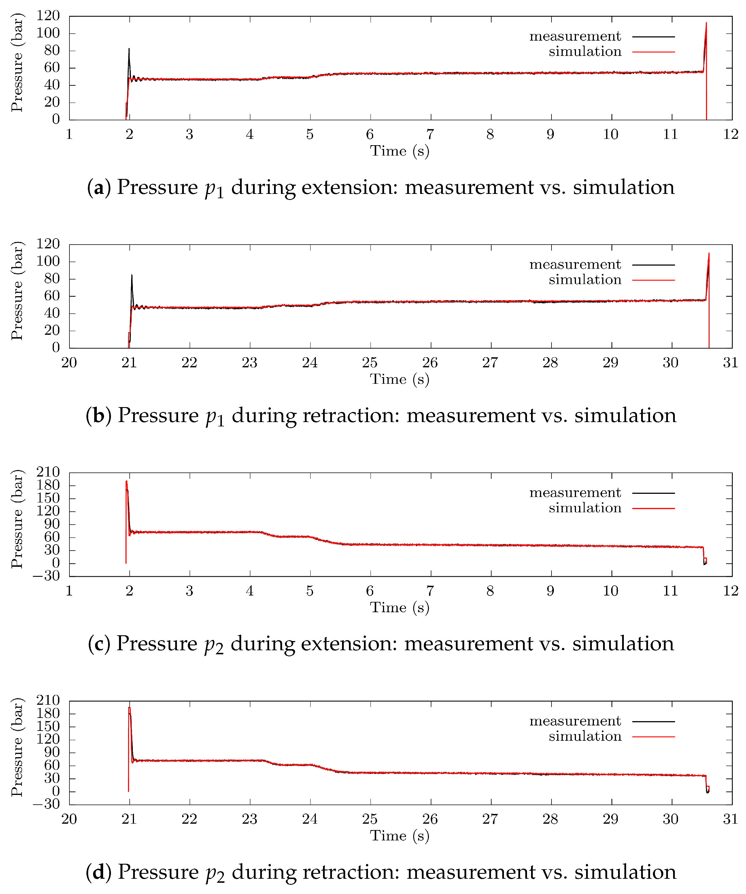
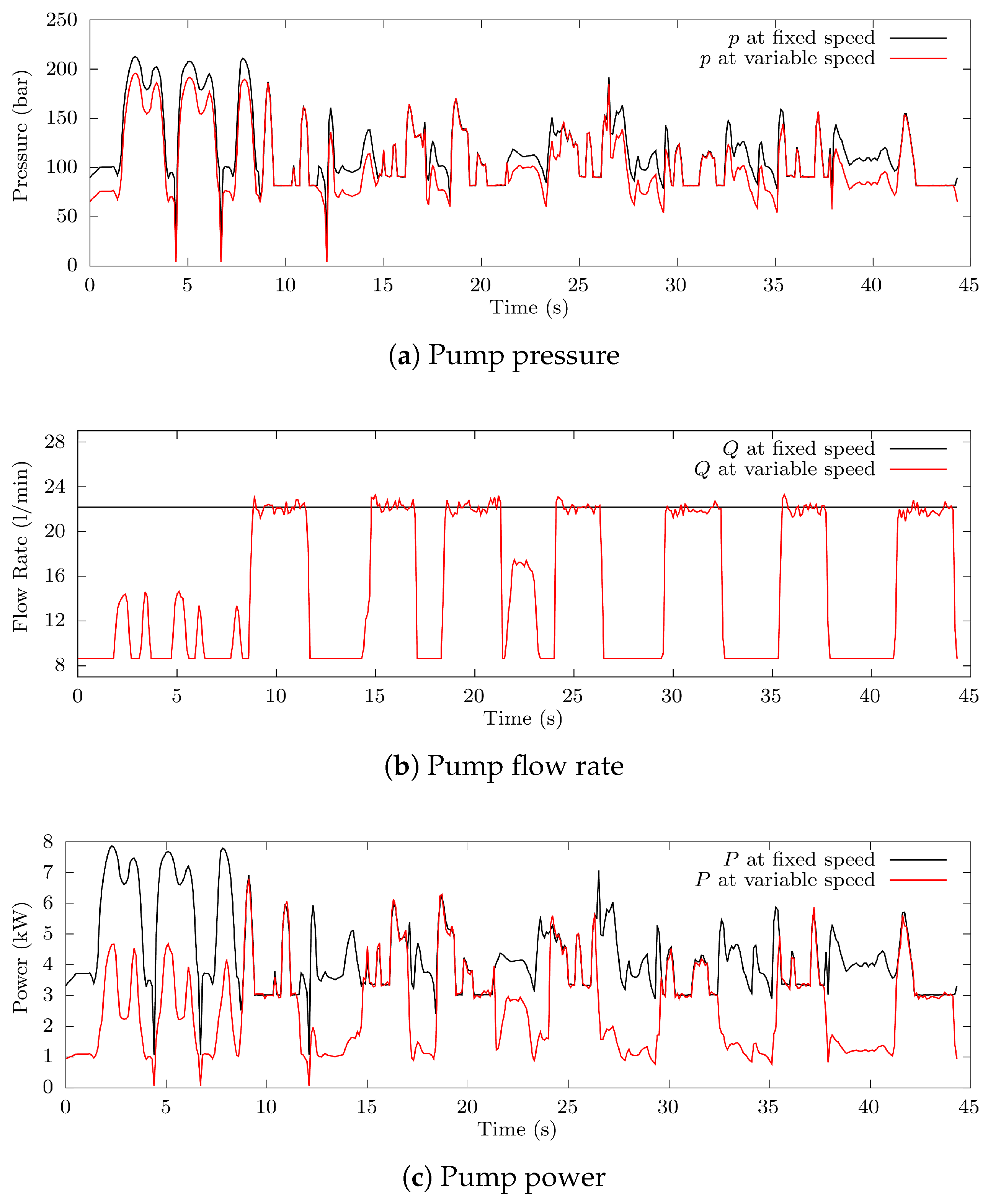
The three configurations are easily achievable in Simulink, with small changes to the model.

The fixed-speed scheme is shown in Figure 2 and represents the conventional configuration of the implement.

The first electrification scheme is shown in Figure 11 and presents design changes with respect to the original configuration. First, the pump is decoupled from the PTO to enable the application of variable speed. Then, the PTO is connected to a series of an electric generator, rectifier, inverter, and electric motor to drive the pump. It is expected that 48 V and 10 kW are the voltage and the power level of the electrical devices required to achieve variable-speed operation in the considered application. In this first electrification scheme, the hydraulic circuit would remain untouched.

The second electrification scheme is shown in Figure 12 and consists of eliminating the flow divider to decouple the lift and tilt circuits and further improve the system efficiency. This scheme, known as decentralization [33], requires an electric drive (inverter and motor) and a pump for each circuit. The original pump is replaced with two smaller pumps, one for each actuator.

Hydraulic pumps should not be run slower than their designated minimum operating speed. In particular, for fixed displacement pumps, it is advised to operate always at a higher speed than the minimum one to avoid lubrication issues and potential damage.

The original 10.8 cm³/rev fixed displacement pump in Figure 2 and Figure 11 has a minimum operating speed of 800 rpm. In the fixed-speed scheme, the pump speed will be 1950 rpm, and the pump flow rate will be 22.1 L/min, as explained in Section 2.4. In the first electrification speed, the variable-speed operation enables us to decrease the pump speed to 800 rpm when idle, reducing the flow rate to 8.8 L/min accordingly. In the second electrification scheme, the original 10.8 cm³/rev fixed displacement pump is replaced with two identical 6.0 cm³/rev fixed displacement pumps, with a minimum operating speed of 1200 rpm and a minimum flow rate of 7.2 L/min.

The following efficiency values have been assumed for the system components: 94% for the gearbox, 92% for the generator, 95% for the rectifier, 95% for the inverter, and 94% for the motor. It follows that, at fixed speed, only the efficiency of the gearbox (94%) should be considered in the energy assessment computations. At variable speed, the efficiency of the series of gearbox, generator, rectifier, inverter, and motor is 73% ($0.94·0.92·0.95·0.95·0.94=0.73$).

3. Results

This section shows the results obtained with the proposed quasi-static model for both fixed- and variable-speed operations. The model, re-adjusted for the circuit updates in the first and the second electrification schemes, is used to assess energy savings across all three configurations. The parameters of the model have been set to match with the tractor implement under study. Regarding the model inputs, the actuators cycles (force and speed) have been selected from the measurement campaign done on the implement. The data logs presented in Section 2.2 have been combined as follows:

• Outdoor test for lift (Figure 5) + indoor test for tilt (Figure 4).
• Indoor test for lift (Figure 3) + indoor test for tilt (Figure 4).

Figure 13 shows the results of the quasi-static model for the land leveler application combining the outdoor (field) test for the lift cylinder and the indoor test for the tilt cylinder.

First, the pump pressure and pump flow rate are calculated in the case of fixed-speed operation (depicted in black). Then, they are computed as though the pump were able to operate at variable speed (depicted in red), adopting the first electrification scheme. Comparing the pump flow rate p at fixed and variable speed, it is possible to notice an offset up to 24.4 bar between the two, with the pressure required at variable speed being lower, on average, than the pressure required at fixed speed. The results regarding the flow rate Q accentuate the distinction between the two modes of operation as follows: the flow rate at fixed speed is constantly equal to 22.1 L/min, while the flow rate at variable speed is in between 8.8 and 23.35 L/min, with the average value being equal to 14.87 L/min. It turns out that the variable-speed operation is able to satisfy the same load requests defined in Figure 4 and Figure 5, with lower pressure and flow rate at the pump side compared to the fixed-speed operation. In terms of hydraulic power, the last subplot of Figure 13 shows the noticeable difference of power required by the pump switching from a fixed-speed to a variable-speed operation mode as follows: the maximum value decreases from 7.86 to 6.79 kW, and the average value decreases from 4.3 to 2.6 kW. The average mechanical power at the PTO can be computed by dividing 4.3 kW by 0.94 (i.e., the gearbox efficiency), leading to 4.57 kW at fixed-speed operation. In case of variable speed, achievable with the electrification scheme in Figure 11, the power computation needs to take into account the additional electrical components. Assuming that the series of gearbox, generator, rectifier, inverter, and motor has an overall efficiency of 73%, it follows that the average mechanical power at the PTO is equal to 2.6/0.73 = 3.54 kW at variable-speed operation. The energy consumption can be assessed by multiplying the average power for the test time which is 44.3 s, leading to 202.65 kJ at fixed speed and 157 kJ at variable speed. The energy savings through partial electrification are equal to 45.65 kJ, which correspond to an efficiency improvement of 22.5%. The results of this example are stored in

Table 1. Assessment of energy savings with the first electrification scheme.

Lift	Tilt	PTO Total Energy at Fixed Speed (Original Circuit)	PTO Total Energy at Variable Speed (First Electrification Scheme)	Energy Savings
Field test	Indoor test	202.65 kJ	157 kJ	22.5%
Indoor test	Indoor test	146.09 kJ	132.76 kJ	9.1%

as the first entry. The second entry of the table represents the second combination based on the available recorded data, where both lift and tilt actuators were tested indoor. In this scenario, the quasi-static model with the two actuators operating simultaneously in the presence of the flow divider assessed energy savings of 9.1%.

The results of the second electrification scheme are presented in

Table 2. Assessment of energy savings with the second electrification scheme.

Lift	Tilt	PTO Total Energy at Fixed Speed Centralized (Original Circuit)	PTO Total Energy at Variable Speed Decentralized (Second Electrification Scheme)	Energy Savings
Field test	Indoor test	202.65 kJ	94.36 kJ	53.4%
Indoor test	Indoor test	146.09 kJ	80.31 kJ	45%

. The first entry refers to the first test case (outdoor test for lift + indoor test for tilt). The pump for the lift circuit absorbs an average mechanical power of 1.11 kW, while the pump for the tilt circuit absorbs an average mechanical power of 0.45 kW. Assuming that the inverters and the e-motors have an efficiency of 95% and 94%, it can be computed that the average power consumption of the two electric drives is in total (1.11 + 0.45)/(0.95 · 0.94) = 1.75 kW. Furthermore, considering the assumed efficiencies of the gearbox, generator, and rectifier, it follows that the total average power at the PTO is 2.13 kW, which, multiplied by the 44.3 s of the test, leads to a total energy consumption of 94.36 kJ. The difference between the total energy with the original configuration is 108.29 kJ, corresponding to energy savings of 53.4%. The second entry of Table 2 relates to the test case in which both the lift and tilt actuator cycles were recorded indoor. The pump for the lift circuit absorbs an average power of 0.88 kW, while the pump for the tilt circuit absorbs an average power of 0.45 kW, with a total energy consumption at the PTO of 80.31 kJ. The difference between the total energy with the original configuration is 65.78 kJ, corresponding to energy savings of 45%.

4. Discussion

The obtained results are discussed in the following. The first key consideration is the reduction in flow rate, which represents a substantial improvement in energy efficiency compared to the state-of-the-art load sensing system at fixed speed. Accordingly, there is a reduction in pump pressure and hydraulic power. In the first electrification scheme, the variable-speed operation decreases the pump speed to 800 rpm at idle, accordingly reducing the flow rate to 8.8 L/min, as shown in Figure 13. In the second electrification scheme, the minimum operating speed of 6.0 cm³/rev fixed displacement pumps is 1200 rpm, while their minimum flow rate is 7.2 L/min.

The second key consideration is that a further improvement in the energy savings could be achieved with the second electrification scheme. As explained in Section 2.4, a noticeable pressure drop occurs across the flow divider. Consequently, eliminating the flow divider to decouple the lift and tilt circuits could yield significant benefits in terms of energy efficiency. Moreover, hydraulic circuits with decentralized pumps (one pump per actuator) are more efficient than load-sensing systems with a single large pump because they allow each actuator to operate at its optimal pressure, eliminating energy waste from maintaining unnecessarily high pressure for the entire system.

Comparing the results of Table 1 with Table 2, it turns out that the second electrification scheme enables higher energy savings. The efficiency of the electrical devices (generator, rectifier, inverters, and motors) has been considered in this work to yield a consistent energy assessment of the system in comparison with the traditional circuit configuration. A comprehensive analysis performed by implement manufacturers should take into account the higher expenses related to the additional electrical hardware, but it should also consider the energy prices and the potential long-term cost savings. A feasibility evaluation of hybrid electric agricultural tractors based on life cycle cost analysis is performed in [9]. In summary, electrified implements have the benefit of enabling higher efficiency than traditional non-electrified configurations, reducing emissions. Furthermore, they are projected to play a key role in the future by facilitating more autonomous and precise agricultural practices.

5. Conclusions

This study has presented a quasi-static model for assessing potential energy savings through the partial electrification of a land leveler implement. The results demonstrate that the proposed electrification schemes lead to substantial improvements in system efficiency. In particular, the first electrification scheme (pump driven by a variable-speed e-motor, with no changes in the hydraulic circuit) guarantees energy savings of 9.1–22.5% with the considered test cases. The second electrification scheme (decentralization of the hydraulic system and removal of the flow divider) enables energy savings of 45–53.4% compared to the original setup. These findings highlight the significant potential of partial electrification in improving the energy efficiency of agricultural implements. Future work should involve field testing of land leveler prototypes implementing one or both proposed electrification schemes to validate the model’s predictions and assess real-world energy savings.

References

1. Moreda, G.P.; noz García, M.A.M.; Barreiro, P. High voltage electrification of tractor and agricultural machinery—A review. Energy Convers. Manag. 2016, 115, 117–131. [Google Scholar] [CrossRef]
2. Scolaro, E.; Beligoj, M.; Estevez, M.P.; Alberti, L.; Renzi, M.; Mattetti, M. Electrification of Agricultural Machinery: A Review. IEEE Access 2021, 9, 164520–164541. [Google Scholar] [CrossRef]
3. Un-Noor, F.; Wu, G.; Perugu, H.; Collier, S.; Yoon, S.; Barth, M.; Boriboonsomsin, K. Off-Road Construction and Agricultural Equipment Electrification: Review, Challenges, and Opportunities. Vehicles 2022, 4, 780–807. [Google Scholar] [CrossRef]
4. Mocera, F.; Somà, A.; Martelli, S.; Martini, V. Trends and Future Perspective of Electrification in Agricultural Tractor-Implement Applications. Energies 2023, 16, 6601. [Google Scholar] [CrossRef]
5. Buning, E.A. Electric drives in agricultural machinery—Approach from the tractor side. J. Agric. Eng. 2010, 47, 30–35. [Google Scholar]
6. Tritschler, P.J.; Bacha, S.; Rullière, E.; Husson, G. Energy management strategies for an embedded fuel cell system on agricultural vehicles. In Proceedings of the The XIX International Conference on Electrical Machines—(ICEM 2010), Rome, Italy, 6–8 September 2010; pp. 1–6. [Google Scholar]
7. Stempfer, G.; Bebeti, M.; Himmelsbach, R.; Volpert, B. Electrification in agricultural engineering technologies and synergies. Atzoffhighway Worldw. 2017, 10, 66–69. [Google Scholar] [CrossRef]
8. Minav, T.; Lehmuspelto, T.; Sainio, P.; Pietola, M. Series Hybrid Mining Loader with Zonal Hydraulics. In Proceedings of the 10th International Fluid Power Conference, Dresden, Germany, 8–10 March 2016; pp. 211–224. [Google Scholar]
9. Beligoj, M.; Scolaro, E.; Alberti, L.; Renzi, M.; Mattetti, M. Feasibility Evaluation of Hybrid Electric Agricultural Tractors Based on Life Cycle Cost Analysis. IEEE Access 2022, 10, 28853–28867. [Google Scholar] [CrossRef]
10. Perez Estevez, M.A.; Melendez Frigola, J.; Armengol Llobet, J.; Alberti, L.; Renzi, M. Optimal design of a series hybrid powertrain for an agricultural tractor. Energy Convers. Manag. X 2024, 24, 100789. [Google Scholar] [CrossRef]
11. Mattetti, M.; Annesi, G.; Intrevado, F.P.; Alberti, L. Investigating the efficiency of hybrid architectures for agricultural tractors using real-world farming data. Appl. Energy 2025, 377, 124499. [Google Scholar] [CrossRef]
12. Renius, K.T. Fundamentals of Tractor Design; Springer Charm: Berlin/Heidelberg, Germany, 2020. [Google Scholar]
13. Stoss, K.J.; Sobotzik, J.; Shi, B.; Kreis, E.R. Tractor Power for Implement Operation-Mechanical, Hydraulic, and Electrical: An Overview. In Proceedings of the 2013 Agricultural Equipment Technology Conference, Kansas City, MO, USA, 28–30 January 2013; American Society of Agricultural and Biological Engineers (ASABE): St. Joseph, MI, USA, 2013. [Google Scholar]
14. Gonzalez de-Soto, M.; Emmi, L.; Benavides, C.; Garcia, I.; Gonzalez de-Santos, P. Reducing air pollution with hybrid-powered robotic tractors for precision agriculture. Biosyst. Eng. 2016, 143, 79–94. [Google Scholar] [CrossRef]
15. Engström, J.; Lagnelöv, O. An Autonomous Electric Powered Tractor–Simulation of All Operations on a Swedish Dairy Farm. J. Agric. Sci. Technol. 2018, 8, 182–187. [Google Scholar] [CrossRef]
16. Lajunen, A.; Sainio, P.; Laurila, L.; Pippuri-Mäkeläinen, J.; Tammi, K. Overview of Powertrain Electrification and Future Scenarios for Non-Road Mobile Machinery. Energies 2018, 11, 1184. [Google Scholar] [CrossRef]
17. Pickel, P. Electricity for tractors and tractor-implement systems. In Proceedings of the 29th Members Meeting, Hannover, Germany, 10–11 November 2019. [Google Scholar]
18. Cisternas, I.; Velásquez, I.; Caro, A.; Rodríguez, A. Systematic literature review of implementations of precision agriculture. Comput. Electron. Agric. 2020, 176, 105626. [Google Scholar] [CrossRef]
19. Prabhakaran, A.; Chithra Lekshmi, K.S.; Janarthanan, G. Advancement of data mining methods for improvement of agricultural methods and productivity. In Artificial Intelligence in Data Mining; Binu, D., Rajakumar, B.R., Eds.; Academic Press: Cambridge, MA, USA, 2021; pp. 199–221. [Google Scholar]
20. Belforte, G.; Deboli, R.; Gay, P.; Piccarolo, P.; Ricauda Aimonino, D. Robot Design and Testing for Greenhouse Applications. Biosyst. Eng. 2006, 95, 309–321. [Google Scholar] [CrossRef]
21. Escolà, A.; Rosell-Polo, J.R.; Planas, S.; Gil, E.; Pomar, J.; Camp, F.; Llorens, J.; Solanelles, F. Variable rate sprayer. Part 1—Orchard prototype: Design, implementation and validation. Comput. Electron. Agric. 2013, 95, 122–135. [Google Scholar] [CrossRef]
22. Bechar, A.; Vigneault, C. Agricultural robots for field operations: Concepts and components. Biosyst. Eng. 2016, 149, 94–111. [Google Scholar] [CrossRef]
23. Comba, L.; Biglia, A.; Sopegno, A.; Grella, M.; Dicembrini, E.; Ricauda Aimonino, D.; Gay, P. Convolutional Neural Network Based Detection of Chestnut Burrs in UAV Aerial Imagery. In Proceedings of the AIIA 2022: Biosystems Engineering Towards the Green Deal, Palermo, Italy, 19–22 September 2022; Ferro, V., Giordano, G., Orlando, S., Vallone, M., Cascone, G., Porto, S.M.C., Eds.; Springer International Publishing: Cham, Switzerland, 2023; pp. 501–508. [Google Scholar]
24. Hahn, K. High Voltage Electric Tractor-Implement Interface. SAE Int. J. Commer. Veh. 2008, 1, 383–391. [Google Scholar] [CrossRef]
25. Rauch, N. Experiences and visions of an implement manufacturer. Agric. Eng. Today 2010, 35, 3–9. [Google Scholar]
26. Rahe, F.; Resch, R. Electrification of Agricultural Machinery From the Perspective of an Implement Manufacturer. In Proceedings of the 9th AVL International Commercial Powertrain Conference 2017, Messe Congress Graz, Austria, 10–11 May 2017. [Google Scholar]
27. Bals, R.; Jünemann, D.; Berghaus, A. Partial Electrification of an Agricultural Implement. Atzheavy Duty Worldw. 2019, 12, 38–41. [Google Scholar] [CrossRef]
28. Varani, M.; Mattetti, M.; Molari, G. Performance Evaluation of Electrically Driven Agricultural Implements Powered by an External Generator. Agronomy 2021, 11, 1447. [Google Scholar] [CrossRef]
29. Magnusson, J.; Eric, P. Electrifying Agricultural Implements: A Study of Design Implications of Electrification. Master’s Thesis, Jönköping University, Jönköping, Sweden, 2023. [Google Scholar]
30. Tian, X.; Jenkins, R.; Lengacher, J.; Vacca, A.; Fiorati, S.; Pintore, F.; Cristofori, D. An Analysis of Mixed Hydraulic and Electric Configurations for the Actuation of Tractor Auxiliary and Implement Functions to Reduce Power Consumption. In Proceedings of the LAND.TECHNIK AgEng 2023, Hannover, Germany, 10 November 2023; pp. 1–14. [Google Scholar]
31. Grossi, F.; Cittadella, M.; Biagiotti, L.; Mariniello, C. Improving Efficiency of Farming Tractor Implement by Electrification. In Proceedings of the 2024 IEEE Vehicle Power and Propulsion Conference (VPPC), Washington, DC, USA, 7–10 October 2024; pp. 1–6. [Google Scholar]
32. Khatti, R.; Plate, J. Allis-Chalmers Load-Sensitive Hydraulic System for Tractor-Implement Control. Trans. ASABE 1974, 17, 851–855. [Google Scholar] [CrossRef]
33. Beligoj, M.; Zava, M.; Alberti, L.; Termini, A. Hydraulics Decentralization on a Mobile Crane. In Proceedings of the 2022 Second International Conference on Sustainable Mobility Applications, Renewables and Technology (SMART), Cassino, Italy, 23–25 November 2022; pp. 1–9. [Google Scholar]
34. Vacca, A.; Franzoni, G. Hydraulic Fluid Power: Fundamentals, Applications, and Circuit Design; Wiley: Hoboken, NJ, USA, 2021. [Google Scholar]
Figure 1. Land leveler under study.
Energies 18 02766 g001
Figure 2. Hydraulic circuit of the land leveler.
Energies 18 02766 g002
Figure 3. Lift actuator cycle (indoor test measurements).
Energies 18 02766 g003
Figure 4. Tilt actuator cycle (indoor test measurements).
Energies 18 02766 g004
Figure 5. Lift actuator cycle (outdoor test measurements).
Energies 18 02766 g005
Figure 6. Scheme of a linear actuator with CBV.
Energies 18 02766 g006
Figure 7. Block diagram of the quasi-static model in the case of one cylinder.
Energies 18 02766 g007
Figure 8. Lift actuator pressures for model accuracy evaluation.
Energies 18 02766 g008
Figure 9. Flow divider (FD) basic schematic, operation, and pressure drop.
Energies 18 02766 g009
Figure 10. Block diagram of the extended quasi-static model including the flow divider.
Energies 18 02766 g010
Figure 11. Hydraulic circuit of the land leveler—first electrification scheme.
Energies 18 02766 g011
Figure 12. Hydraulic circuit of the land leveler—second electrification scheme.
Energies 18 02766 g012
Figure 13. Simulation results: pump pressure, flow rate, and power (outdoor test for lift + indoor test for tilt).
Energies 18 02766 g013