Steady-State Model Enabled Dynamic PEMFC Performance Degradation Prediction via Recurrent Neural Network

Abstract

Proton exchange membrane fuel cells (PEMFC), distinguished by rapid refueling capability and zero tailpipe emissions, have emerged as a transformative energy conversion technology for automotive applications. Nevertheless, their widespread commercialization remains constrained by technical limitations mainly in operational longevity. Precise prognostics of performance degradation could enable real-time optimization of operation, thereby extending service life. This investigation proposes a hybrid prognostic framework integrating steady-state modeling with dynamic condition. First, a refined semi-empirical steady-state model was developed. Model parameters’ identification was achieved using grey wolf optimizer. Subsequently, dynamic durability testing data underwent systematic preprocessing through a correlation-based screening protocol. The processed dataset, comprising model-calculated reference outputs under dynamic conditions synchronized with filtered operational parameters, served as inputs for a recurrent neural network (RNN). Comparative analysis of multiple RNN variants revealed that the hybrid methodology achieved superior prediction fidelity, demonstrating a root mean square error of 0.6228%. Notably, the integration of steady-state physics could reduce the RNN structural complexity while maintaining equivalent prediction accuracy. This model-informed data fusion approach establishes a novel paradigm for PEMFC lifetime assessment. The proposed methodology provides automakers with a computationally efficient framework for durability prediction and control optimization in vehicular fuel cell systems.

1. Introduction

As global energy systems transition toward carbon neutrality, hydrogen integration with renewable power generation has been recognized as a strategic enabler for sustainable energy infrastructure [1]. Proton exchange membrane fuel cells (PEMFC), which electrochemically convert hydrogen into electricity with water as the sole byproduct, represent a critical energy conversion technology. Their superior energy density, exceptional conversion efficiency, rapid refueling capability, and emission-free operation position PEMFC as particularly advantageous for heavy-duty transportation applications requiring extended operational range [2]. Nevertheless, persistent degradation mechanisms during operational cycling substantially limit service lifetimes, elevating maintenance costs and total ownership expenditures [3,4]. Current research focuses on two complementary longevity enhancement pathways: fundamental material-structural innovations and operational optimization. At the component level, advances in membrane electrode assembly design, corrosion-resistant bipolar plates, and durable balance-of-plant subsystems have demonstrated potential for intrinsic durability improvements [5]. At the system level, empirical studies reveal strong correlations between PEMFC degradation rates and transient load profiles characteristic of vehicular duty cycles [6,7]. This has motivated the implementation of hybridized powertrain architectures in fuel cell electric vehicles (FCEV), where intelligent energy management strategies (EMS) coordinate power allocation between PEMFC stacks and secondary energy storage devices. Such strategies enable load-leveling operations that simultaneously enhance energy efficiency and mitigate electrochemical degradation [8]. However, developing health-aware EMS necessitates high-fidelity degradation models that capture complex interplay between operational parameters and failure modes.

The degradation of PEMFC manifests through interdependent mechanical and electrochemical degradation mechanisms. This complexity necessitates a multidisciplinary analytical framework integrating continuum mechanics, electrochemical kinetics, and nonequilibrium thermodynamics to comprehensively characterize degradation trajectories [9,10,11]. However, the quantitative deconvolution of individual degradation contributors—including asymmetric interfacial stress distribution between electrodes, catalyst layer Ostwald ripening, carbon support oxidation, and membrane chemical decomposition—presents formidable technical challenges. Consequently, the operational voltage signature has emerged as the principal diagnostic metric due to its noninvasive monitoring capability and direct correlation with performance loss. Industry-standard durability assessments typically define a 10% voltage decay at rated operating conditions as the failure threshold for automotive PEMFC stacks [12]. Current prognostic methodologies leverage both accelerated stress testing protocols under laboratory-controlled environments and field-monitored vehicular operational datasets to establish degradation prediction frameworks.

Chen et al. [7] systematically captured operational profiles from a fuel cell electric bus fleet, classifying four distinct duty-cycle archetypes through clustering analysis. Their empirical statistical framework quantified voltage degradation rates for each operational pattern, establishing a computationally tractable methodology for automotive PEMFC performance prognosis. Bressel et al. [13] advanced a dynamic polarization curve model parameterized by four degradation-sensitive variables: open-circuit voltage, ohmic resistance, exchange current density, and oxygen mass transport limitation. A state-space formulation coupled with an adaptive extended Kalman filtering framework enabled robust state-of-health (SOH) estimation under transient operating conditions. Jouin et al. [14] enhanced polarization modeling fidelity through mechanistic decomposition of aging phenomena, employing multiphysics-informed temporal functions (linear, exponential, and bi-exponential) to characterize degradation trajectories of membrane hydration and catalyst activity. Li et al. [15] focused on quasi-stationary PEMFC operation in urban bus applications, leveraging electrochemical surface area (ECSA) attenuation as the principal degradation proxy. Their exponential decay model correlated ECSA reduction with cumulative operational time under constrained power demand profiles. Hu et al. [16] extended this paradigm by integrating voltage recovery phenomena during idling phases, though both approaches exhibited practical constraints tied to their narrow operational envelopes—specifically, PEMFC operation restricted to certified reliability zones with minimized load fluctuations [15,16].

To overcome scenario-specific limitations, Zhang et al. [17] pioneered a frequency-domain degradation analysis framework. By applying discrete Fourier transforms to time-series voltage/current profiles, they derived spectral energy distribution metrics that were subsequently incorporated into modified polarization equations. This signal processing-enhanced methodology demonstrated improved generalization capability across diverse load cycles while maintaining prognostic accuracy.

Besides the model-based approach, data-driven methods have emerged recently for their ability to model the high-order nonlinearity of degradation [17]. Cheng et al. [18] proposed a method of combining the least square support vector machine (LSSVM) and regularized particle filter (RPF). The RPF method received the preliminary prediction results of LSSVM and output the performance degradation results in the format of probability distribution considering the uncertainty characterization. Ma et al. [19] developed a two-dimensional grid long short-term memory (LSTM) recurrent neural network (RNN) to predict performance degradation. The 58% aging data of Ballard NEXA and 69% aging data of PM200 fuel cell were used to train the RNN. Both datasets achieved a good prediction performance. Liu et al. [20] proposed a sequence hybrid method to predict performance degradation. In the first phase of the sequence method, an adaptive neuro-fuzzy inference system was trained to predict the long-term degradation trend. The model-based method coupled with the Kalman filter predicted the single-step output. Zuo et al. [21] proposed and compared four RNN-based methods, i.e., LSTM, attention-based LSTM, gate-recurrent unit (GRU) recurrent neural network, and attention-based GRU, to predict performance degradation. The prediction criteria of four methods, measured by root mean square error (RMSE), ranged from 0.003831 to 0.017637 on two datasets. Other neural-network-based methods, for instance, echo state network (ESN) [22,23], GRU [24,25], bi-direction GRU [26,27], bi-direction LSTM [28,29,30], organic grey neural network [31], and Bayesian RNN [32], were deployed. Yue et al. [22] introduced the optimization of sliding window length to the ESN-based method. The ESN-based method achieved an excellent prediction performance (0.017, measured by RMSE), only consuming 13.8% of computation loads compared to the stacked LSTM [33]. Tao et al. [25] combined the two-dimensional convolutional neural network (CNN) and GRU to predict performance degradation. Using the dataset provided by [34], the best RSME of the proposed method achieved 0.0103516. Wilberforce et al. [35] explored the combination of CNN and bi-direction RNN. Wang et al. [36] combined the semi-empirical model and the semi-recurrent sliding window method developed by [37] to predict the performance degradation. The weighted average of the two models’ outputs calculated the prediction result. Furthermore, the evolving paradigm of physics-informed neural networks (PINNs) has been progressively adapted for PEMFC degradation prognostics. Liu et al. [38] employed equivalent circuit models as the embedded physical constraints, developing physics-constrained composite loss functions that explicitly penalize deviations from electrochemical impedance spectroscopy-derived aging patterns. Concurrently, Ko et al. [39] implemented a hybrid architecture where simplified semi-empirical voltage models govern the regularization terms within the loss function space. The fundamental mechanism of PINNs resides in this strategic incorporation of physical model residuals as differentiable regularizers during the optimization process: the data-driven predictions dynamically compensate for discrepancies in first-principles simulations through gradient-based co-optimization of a composite loss function. This dual-constrained optimization framework ensures simultaneous minimization of empirical errors and thermodynamic inconsistencies, effectively creating a synergistically constrained solution manifold that adheres to both observational data and domain knowledge.

While substantial progress has been made in proton exchange membrane fuel cell (PEMFC) degradation prognostics, three critical limitations persist in current methodologies:

• Modeling insufficiency: Existing semi-empirical frameworks inadequately capture coupled electrochemical–physical degradation mechanisms, particularly under transient operational regimes.
• Feature ambiguity: Data-driven approaches frequently employ heuristic feature selection without systematic quantification of degradation-relevant feature vectors, limiting their capacity to resolve high-order nonlinear degradation dynamics.
• Integration naivety: Prevailing hybrid methodologies often adopt linear additive fusion frameworks that fail to exploit synergistic interactions between physics-based models and machine learning architectures.

This investigation addresses these critical gaps through three methodological innovations:

• Development of a self-consistent electrochemistry-explicit model integrating Nernst–Planck transport dynamics with Butler–Volmer reaction kinetics for enhanced mechanistic fidelity.
• Rather than embedding physics residuals as regularization terms, implementation of physics-informed feature engineering that systematically extracts degradation-sensitive parameters through thermodynamic irreversibility analysis.
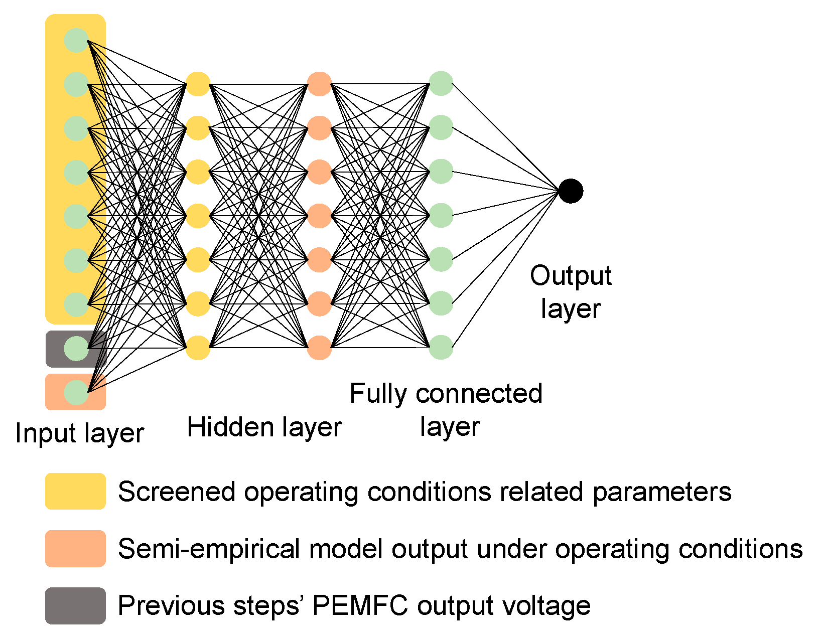
• Creation of a nonlinear co-learning framework where semi-empirical model outputs are encoded as latent states within RNN architectures through attention-based fusion mechanisms.

The paper is structured as follows. Section 2 details the reformulated PEMFC degradation model and its parameter identification via an enhanced grey wolf optimization (GWO) algorithm with adaptive convergence criteria. Section 3 introduces the proposed hybrid RNN architecture, emphasizing the bidirectional encoding of electrochemical principles into temporal learning layers. Comparative experimental results and failure mode sensitivity analyses are presented in Section 4, followed by conclusions outlining industrial implementation pathways.

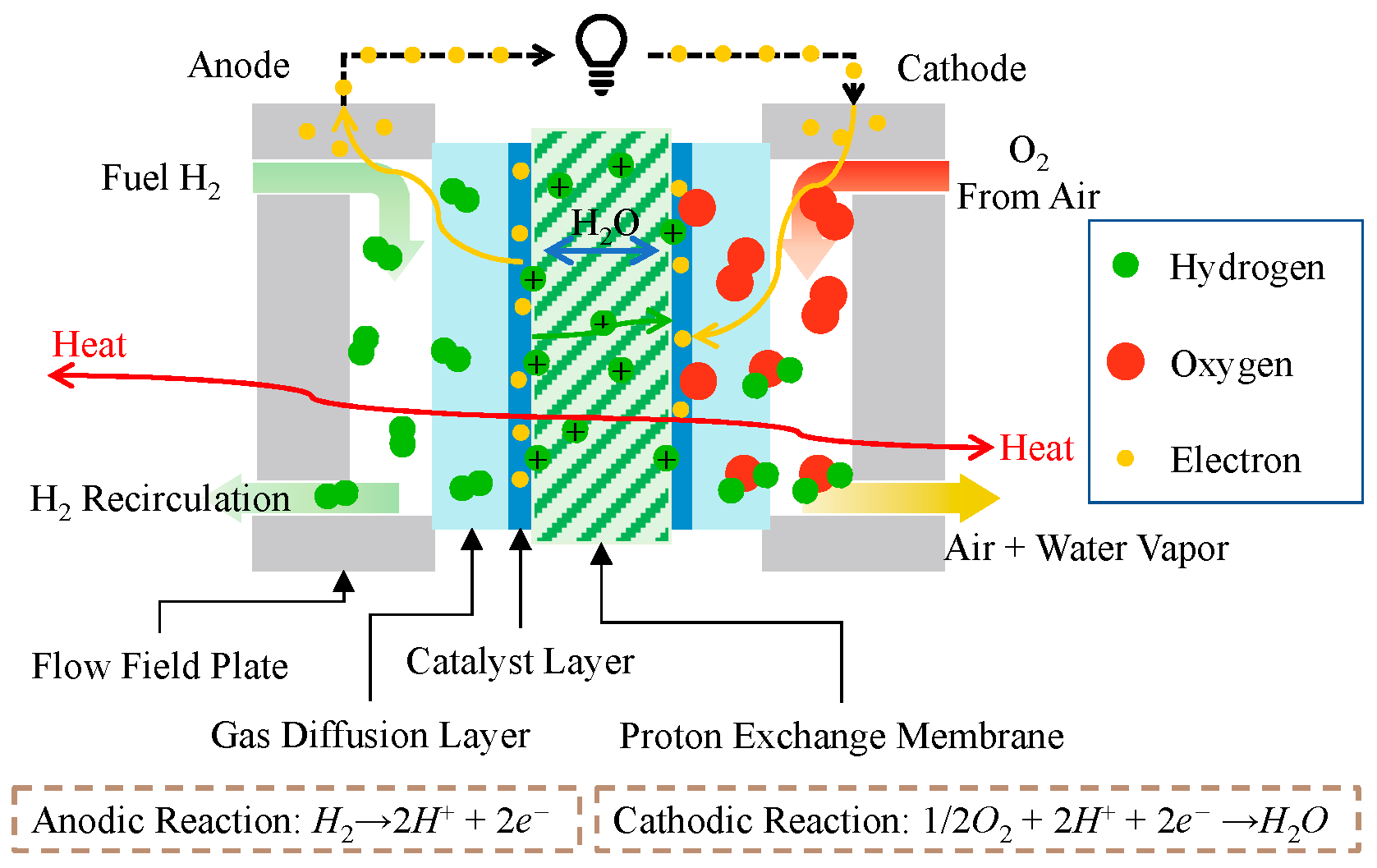
2. Self-Consistent Semi-Empirical Model

Figure 1 presents a generic schematic representation of a PEMFC architecture. The fundamental electrochemical mechanism involves the oxidation of hydrogen at the anode and the reduction of oxygen at the cathode: hydrogen molecules are electrochemically oxidized at the anode catalyst layer, releasing protons that migrate through the membrane while electrons traverse the external circuit. Concurrently, oxygen molecules derived from ambient air are reduced at the cathode catalyst layer, combining with migrated protons and electrons to form water through the oxygen reduction reaction.

The semi-empirical PEMFC modeling framework synergistically integrates physicochemical mechanisms with empirical parameter optimization. By calibrating critical kinetic descriptors through experimental datasets, this methodology addresses inherent limitations of theoretical models in capturing real-world operational complexities. Through its macro-empirical formalism for polarization curve characterization, the model achieves a critical balance between computational tractability and operational fidelity, thereby demonstrating exceptional practical utility for system-level performance prediction and optimization.

2.1. Semi-Empirical Model of PEMFC

The semi-empirical model forms the foundation of PEMFC modeling. The single cell’s voltage is described by the combination of thermodynamic potential (E_Nernst), ohmic loss (η_ohmic), concentration loss (η_conc), and activation loss (η_act).

$$V_{cell}=E_{Nernst}-{\eta }_{ohmic}-{\eta }_{conc}-{\eta }_{act},$$

(1)

The thermodynamic potential is related to the operating temperature and the partial pressure of hydrogen and oxygen.

$$E_{Nernst}=1.229-8.46\times {10}^{-4}\left(T-298.15\right)+{\displaystyle \frac{RT}{nF}}\left(\ln \left(P_{H_2}\right)+{\displaystyle \frac{1}{2}}\ln \left(P_{O_2}\right)\right),$$

(2)

In the PEMFC reaction mechanism, the formation of each water molecule necessitates the consumption of one hydrogen molecule and the transfer of two electrons through the external circuit, thereby establishing the electron transfer coefficient n = 2. As illustrated in Figure 1, the stoichiometric reaction involves half an oxygen molecule reacting with one hydrogen molecule. This stoichiometry necessitates the inclusion of a 1/2 prefactor in the oxygen partial pressure term of the Nernstian formulation. Through logarithmic transformation, this prefactor is analytically extracted, yielding a coefficient of 1/2 ln(P_O2) in the final thermodynamic expression. The P_H2 is the effective partial pressure of hydrogen, unit in bar. It can be estimated using Equation (3):

$$P_{H2}=0.5\left({\displaystyle \frac{P_{an}}{\exp \left(\frac{1.635i}{T^{1.334}}\right)}}-R{H}_{an}{P}_{sat}\right),$$

(3)

where P_sat (unit, bar) is the vapor saturation pressure in the anode at the PEMFC working temperature T (unit, K), RH is the relative humidity of the anode side, and i is the current density of PEMFC, unit in A/cm².

The effective partial pressure of oxygen (P_O2) in the hydrogen–air fuel cells can be calculated.

$$P_{O2}=P_{ca}-R{H}_{ca}{P}_{sat}-P_{N_2}\exp \left({\displaystyle \frac{0.291i}{T^{0.832}}}\right),$$

(4)

where P_N2 is the anode nitrogen partial pressure. This research estimates the nitrogen partial pressure by the mole fraction (x) of nitrogen in the cathode side.

$$P_{N_2}=x_{N_2}{P}_{ca},$$

(5)

The mole fraction of nitrogen in the cathode is the average of the input and output, marked as superscript in and out.

$$x_{N_2}={\displaystyle \frac{x_{N_2}^{in}+x_{N_2}^{out}}{2}},$$

(6)

Assuming the mole fraction of nitrogen and oxygen in the air is 0.79 and 0.21, the molar fraction of nitrogen in the fully humidified input air can be obtained.

$$x_{N_2}^{in}=\left(1-x_{vap\_sat}\right)\times 0.79,$$

(7)

The mole fraction of nitrogen in the cathode output is related to the air stoichiometry (denoted by λ_air).

$$x_{N_2}^{out}={\displaystyle \frac{1-x_{vap\_sat}}{1+\frac{0.21\left({\lambda }_{air}-1\right)}{0.79{\lambda }_{air}}}},$$

(8)

The mole fraction of vapor in the fully humidified air, x_{vap_sat}, can be calculated.

$$x_{vap\_sat}={\displaystyle \frac{R{H}_{ca}{P}_{sat}}{P_{ca}}},$$

(9)

2.1.1. Ohmic Loss

The ohmic loss models the transport resistance of electrons and protons. The PEMFC voltage drop caused by ohmic loss mainly occurs at the median current density range. Using Ohm’s law, the ohmic loss can be calculated,

$${\eta }_{ohmic}=iA\left(R_{mem}+R_{elec}\right),$$

(10)

where A is the PEMFC active area, unit in cm² and R_mem and R_elec are the modeled resistance of membrane and electronic, which simulates the transport resistance of protons and electrons. The membrane resistance is related to the membrane properties,

$$R_{mem}={\displaystyle \frac{{\rho }_{mem}{l}_{thick}}{A}},$$

(11)

where l_thick is the thickness of the membrane, unit cm. The fitting equation can estimate the membrane-specific resistance, ρ_mem (unit, Ω·cm),

$${\rho }_{mem}={\displaystyle \frac{181.6\left(1+0.03i+0.062{\left(\frac{T}{303}\right)}^2{i}^{2.5}\right)}{\left({\lambda }_{mem}-0.634-3i\right)\exp \left(4.18\frac{T-303}{T}\right)}},$$

(12)

where λ_mem is membrane water content. The value of membrane water content varies in many studies. Therefore, this research treats the λ_mem as an unknown constant parameter to be identified. In addition, the electron resistance is the constant parameter to be determined.

2.1.2. Concentration Loss

The concentration loss occurs at both the anode and cathode sides. Both losses can be estimated using Equation (14),

$${\eta }_{conc}={\eta }_{conc,an}+{\eta }_{conc,ca},$$

(13)

$$\left\{\begin{array}{l}{\eta }_{conc,an}=-{\displaystyle \frac{RT}{n_{an}F}}\ln \left(1-{\displaystyle \frac{i+i_{leak,an}}{i_{lim,an}}}\right)\\ {\eta }_{conc,ca}=-{\displaystyle \frac{RT}{n_{ca}F}}\ln \left(1-{\displaystyle \frac{i+i_{leak,ca}}{i_{lim,ca}}}\right)\end{array}\right.,$$

(14)

where R is the gas constant and i_lim is the limiting current density at both sides, unit A/cm². The leak current density at both anode and cathode sides (i_leak,an and i_leak,ca) were introduced, distinguishing electrode-specific gas crossover effects derived from hydrogen and oxygen partial pressure gradients across the membrane. The reactants pass through the gas diffusion layer (GDL) and reach the catalyst surface, at which the reactants are consumed rapidly for electrochemical reaction. Thus, the concentration of the reactants at the catalyst layer surface is much lower than the concentration at the center of the flow channel. These concentration gradients cause the electrochemical potential to vary. The limiting current density is defined as the current density when the concentration at the catalyst layer surface is zero, i.e., the consumption rate at the catalyst layer equals the diffusion rate through the GDL. The limiting current density can be obtained according to Fick’s law,

$$\left\{\begin{array}{l}{i}_{lim,an}={\displaystyle \frac{n_{an}F{D}_{eff,H_2}{C}_{bulk,H_2}}{\mathrm{10,000}{L}_{GDL,an}}}\\ i_{lim,ca}={\displaystyle \frac{n_{ca}F{D}_{eff,O_2}{C}_{bulk,O_2}}{\mathrm{10,000}{L}_{GDL,ca}}}\end{array}\right.,$$

(15)

where the L_GDL is the length of GDL, unit m, D_eff is the effective diffusion coefficient, unit m²/s, C_bulk is the bulk concentration, unit mol/m³, F is the Faraday constant, the constant 10,000 converts the current density unit to A/cm², and subscriptions H₂ and O₂ denote the reactants hydrogen and oxygen. The effective diffusion coefficient of reactants at the poriferous GDL can be estimated from the linear formula,

$$\left\{\begin{array}{l}{D}_{eff,H_2}=f_{GDL,an}{D}_{bulk,H_2}\\ D_{eff,O_2}=f_{GDL,ca}{D}_{bulk,O_2}\end{array}\right.,$$

(16)

where f_GDL is a parameter to correct the effective diffusion coefficient. Conventional PEMFC voltage modeling paradigms predominantly simplify gas transport in GDL by exclusively employing bulk diffusion coefficients to characterize gaseous diffusion processes. However, the inherent presence of subcontinuum pore structures within porous GDL media, where pore diameters approach molecular mean free path dimensions, mandates substantial downward revision of effective diffusion coefficients. This study innovatively incorporates f_GDL architecture implementing molecular diffusion coefficients, thereby enabling multiscale-accurate resolution of gas transport physics across heterogeneous porous matrices. In this study, f_GDL is the unknown parameter that can be fitted and D_bulk (unit, m²/s) is the bulk diffusion coefficient of reactants, which is related to the working temperature and pressure.

$$\left\{\begin{array}{l}{D}_{bulk,H_2}=6.11\times {10}^{-5}{\left({\displaystyle \frac{T}{273.15}}\right)}^{1.5}{\displaystyle \frac{1}{P_{an}}}\\ D_{bulk,O_2}=1.78\times {10}^{-5}{\left({\displaystyle \frac{T}{273.15}}\right)}^{1.5}{\displaystyle \frac{1}{P_{ca}}}\end{array}\right.,$$

(17)

The bulk concentration of reactants can be calculated by the Equation (18):

$$\left\{\begin{array}{l}{C}_{bulk,H_2}={\displaystyle \frac{n}{V}}=1.01325\times {10}^5{\displaystyle \frac{P_{an}-R{H}_{an}{P}_{sat}}{RT}}\\ C_{bulk,O_2}={\displaystyle \frac{n}{V}}=1.01325\times {10}^5{\displaystyle \frac{P_{ca}-R{H}_{ca}{P}_{sat}-P_{N_2}}{RT}}\end{array}\right.,$$

(18)

The constant 1.01325 × 10⁵ converts the pressure unit to Pa.

2.1.3. Activation Loss

Theoretically, the activation loss occurs at both anode and cathode sides because of the electrode’s kinetics.

$${\eta }_{act}={\eta }_{act,an}+{\eta }_{act,ca},$$

(19)

Based on the Butler–Volmer equation, oxidation and reduction reactions co-occur in the cathode and anode. The current density at the anode and cathode side can be written as Equation (20),

$$\left\{\begin{array}{l}{i}_{an}=i_{0,an}\left(\exp \left({\displaystyle \frac{-n_{an}F{\alpha }_{Rd,an}\left(E_{an}-E_{r,an}\right)}{RT}}\right)-\exp \left({\displaystyle \frac{n_{an}F{\alpha }_{Ox,an}\left(E_{an}-E_{r,an}\right)}{RT}}\right)\right)\\ i_{ca}=i_{0,ca}\left(\exp \left({\displaystyle \frac{-n_{ca}F{\alpha }_{Rd,ca}\left(E_{ca}-E_{r,ca}\right)}{RT}}\right)-\exp \left({\displaystyle \frac{n_{ca}F{\alpha }_{Ox,ca}\left(E_{ca}-E_{r,ca}\right)}{RT}}\right)\right)\end{array}\right.,$$

(20)

where i₀ is the exchange current density, unit A/cm², α_Rd and α_Ox are the coefficient reactions related to charge transfer of reduction and oxidation, and E and E_r are the potential (unit, V) and equilibrium potential (unit, V), respectively. Ideally, the current density of PEMFC equals the anode’s and cathode’s current density.

$$\left|i_{an}\right|=\left|i_{ca}\right|=i,$$

(21)

Considering the oxidation reaction takes dominant on the anode side, and the reduction reaction dominates the cathode side when the PEMFC current density is larger than zero, Equation (20) can be rewritten:

$$\left\{\begin{array}{l}{i}_{an}=-i_{0,an}\exp \left({\displaystyle \frac{n_{an}F{\alpha }_{Ox,an}\left(E_{an}-E_{r,an}\right)}{RT}}\right)\\ i_{ca}=i_{0,ca}\exp \left({\displaystyle \frac{-n_{ca}F{\alpha }_{Rd,ca}\left(E_{ca}-E_{r,ca}\right)}{RT}}\right)\end{array}\right.,$$

(22)

Neither the fuel cell stack nor the membrane is insulated. Leakage of protons and electrons is possible, defined as the leak current density (i_leak) at both sides. In addition, electrons flow out of the anode; thus, the i_an is negative. Therefore, Equation (21) can be rewritten:

$$\left|i_{an}\right|-i_{leak,an}=i_{ca}-i_{leak,ca}=i,$$

(23)

The activation losses at both sides, defined by the difference between potential and equilibrium potential, can be derived from Equations (22) and (23).

$$\left\{\begin{array}{l}{\eta }_{act,an}=E_{an}-E_{r,an}={\displaystyle \frac{RT}{n_{an}F{\alpha }_{Ox,an}}}\ln \left({\displaystyle \frac{i+i_{leak,an}}{i_{0,an}}}\right)\\ {\eta }_{act,ca}=E_{r,ca}-E_{ca}={\displaystyle \frac{RT}{n_{ca}F{\alpha }_{Rd,ca}}}\ln \left({\displaystyle \frac{i+i_{leak,ca}}{i_{0,ca}}}\right)\end{array}\right.,$$

(24)

The exchange current density characterizes the equilibrium condition of reduction and oxidation reactions at both the anode and cathode sides when the PEMFC current density is zero. Hence, the exchange current density can be described from the perspective of oxidation reaction and reduction reaction, respectively, at both the anode (Equation (25)) and cathode (Equation (26)) sides,

$$\begin{array}{l}{i}_{0,an}={\displaystyle \frac{n_{an}F{k}_{B}T}{h}}{C}_{Ox,an}\exp \left({\displaystyle \frac{-\Delta G_{Rd,an}}{RT}}\right)\exp \left({\displaystyle \frac{-n_{an}{\alpha }_{0,Rd,an}F{E}_{r,an}}{RT}}\right)\\ ={\displaystyle \frac{n_{an}F{k}_{B}T}{h}}{C}_{Rd,an}\exp \left({\displaystyle \frac{-\Delta G_{Ox,an}}{RT}}\right)\exp \left({\displaystyle \frac{n_{an}{\alpha }_{0,Ox,an}F{E}_{r,an}}{RT}}\right)\end{array},$$

(25)

$$\begin{array}{l}{i}_{0,ca}={\displaystyle \frac{n_{ca}F{k}_{B}T}{h}}{C}_{Ox,ca}\exp \left({\displaystyle \frac{-\Delta G_{Rd,ca}}{RT}}\right)\exp \left({\displaystyle \frac{-n_{ca}{\alpha }_{0,Rd,ca}F{E}_{r,ca}}{RT}}\right)\\ ={\displaystyle \frac{n_{ca}F{k}_{B}T}{h}}{C}_{Rd,ca}\exp \left({\displaystyle \frac{-\Delta G_{Ox,ca}}{RT}}\right)\exp \left({\displaystyle \frac{n_{ca}{\alpha }_{0,Ox,ca}F{E}_{r,ca}}{RT}}\right)\end{array},$$

(26)

where k_B and h are the Boltzmann constant and Plank constant, respectively, ΔG is the chemical Gibbs free energy, subscriptions Rd and Ox denote the reduction and oxidation reactions, respectively, α₀ is the equilibrium charge coefficient of reduction or oxidation reaction at equilibrium condition, and C is the concentration of the reactants at the electrode. Equations (25) and (26) can be simplified to remain consistent with the domination of oxidation and reduction reactions:

$$\left\{\begin{array}{l}{i}_{0,an}={\displaystyle \frac{n_{an}F{k}_{B}T}{h}}{C}_{Rd,an}\exp \left({\displaystyle \frac{-\Delta G_{Ox,an}}{RT}}\right)\exp \left({\displaystyle \frac{n_{an}{\alpha }_{0,Ox,an}F{E}_{r,an}}{RT}}\right)\\ i_{0,ca}={\displaystyle \frac{n_{ca}F{k}_{B}T}{h}}{C}_{Ox,ca}\exp \left({\displaystyle \frac{-\Delta G_{Rd,ca}}{RT}}\right)\exp \left({\displaystyle \frac{-n_{ca}{\alpha }_{0,Rd,ca}F{E}_{r,ca}}{RT}}\right)\end{array}\right.,$$

(27)

The activation loss can be calculated by combining Equations (24) and (27):

$$\left\{\begin{array}{l}{\eta }_{act,an}={\displaystyle \frac{RT}{n_{an}F{\alpha }_{Ox,an}}}\left(\ln \left(i+i_{leak,an}\right)-\ln \left({\displaystyle \frac{n_{an}F{k}_{B}T}{h}}\right)-\ln \left(C_{Rd,an}\right)+{\displaystyle \frac{\Delta G_{Ox,an}}{RT}}-{\displaystyle \frac{n_{an}{\alpha }_{0,Ox,an}F{E}_{r,an}}{RT}}\right)\\ {\eta }_{act,ca}={\displaystyle \frac{RT}{n_{ca}F{\alpha }_{Rd,ca}}}\left(\ln \left(i+i_{leak,ca}\right)-\ln \left({\displaystyle \frac{n_{ca}F{k}_{B}T}{h}}\right)-\ln \left(C_{Ox,ca}\right)+{\displaystyle \frac{\Delta G_{Rd,ca}}{RT}}+{\displaystyle \frac{n_{ca}{\alpha }_{0,Rd,an}F{E}_{r,ca}}{RT}}\right)\end{array}\right.,$$

(28)

On the anode side, the reactant participating in the reduction reaction is hydrogen, while the reactant on the cathode side is oxygen. In addition, the anode reversible potential is defined as zero. The reversible potential at the cathode side is 1.229 V. Thus, Equation (28) can be simplified:

$$\left\{\begin{array}{l}{\eta }_{act,an}={\displaystyle \frac{RT}{n_{an}F{\alpha }_{Ox,an}}}\left(\ln \left(i+i_{leak,an}\right)-\ln \left({\displaystyle \frac{n_{an}F{k}_{B}T}{h}}\right)-\ln \left(C_H\right)+{\displaystyle \frac{\Delta G_{Ox,an}}{RT}}\right)\\ {\eta }_{act,ca}={\displaystyle \frac{RT}{n_{ca}F{\alpha }_{Rd,ca}}}\left(\ln \left(i+i_{leak,ca}\right)-\ln \left({\displaystyle \frac{n_{ca}F{k}_{B}T}{h}}\right)-\ln \left(C_O\right)+{\displaystyle \frac{\Delta G_{Rd,ca}}{RT}}\right)+{\displaystyle \frac{1.229{\alpha }_{0,Rd,ca}}{{\alpha }_{Rd,ca}}}\end{array}\right.,$$

(29)

The reactant concentration at both sides can be estimated through the operating temperature and reactant partial pressure:

$$\left\{\begin{array}{l}{C}_{H_2}={\displaystyle \frac{P_{H_2}}{5.08\times {10}^6\exp \left(-\frac{498}{T}\right)}}\\ C_{O_2}={\displaystyle \frac{P_{O_2}}{1.09\times {10}^6\exp \left(\frac{77}{T}\right)}}\end{array}\right.,$$

(30)

Combining Equations (1)–(30), a precise semi-empirical model of PEMFC is established. Except for the PEMFC operating conditions, there are 11 unknown parameters to be identified.

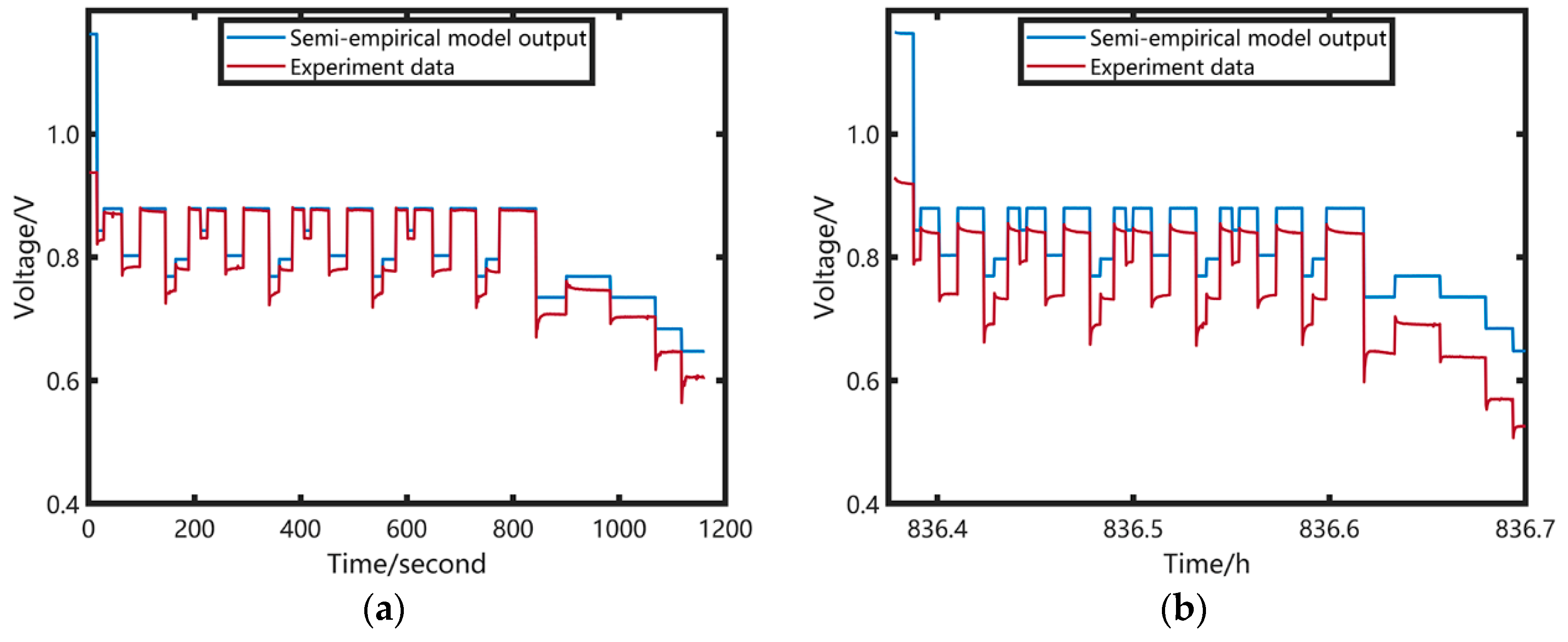
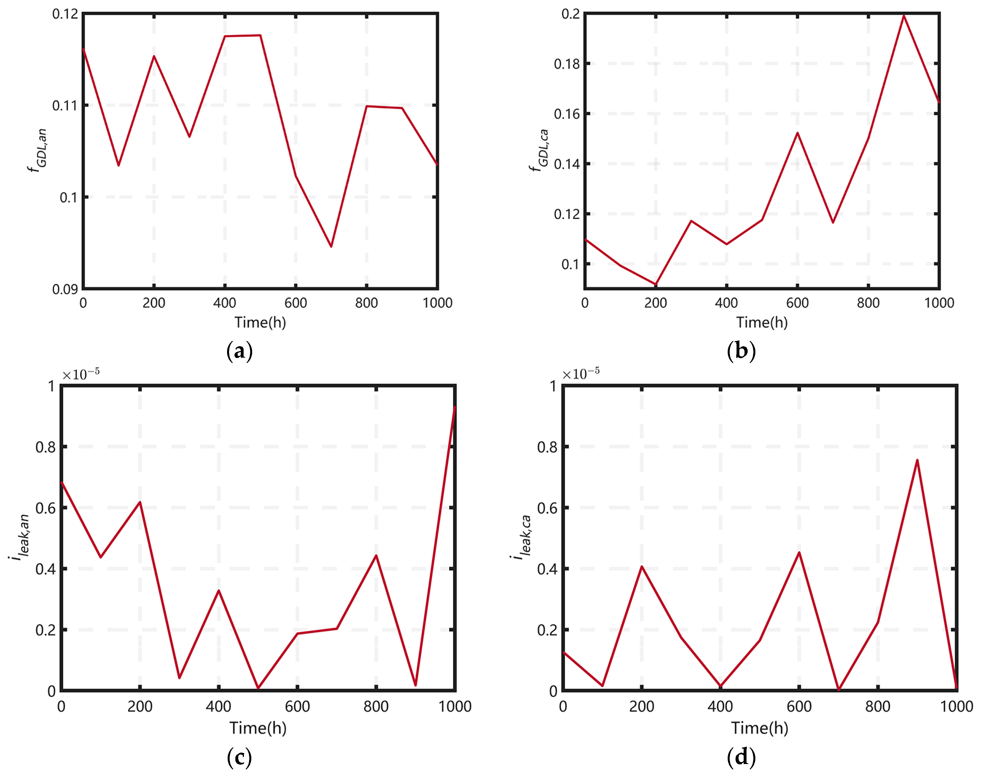
2.2. Model Parameters Identification and Analysis

Neither the stack nor the components manufacturer of PEMFC would report the related parameters. For instance, the coefficients to correct diffusion rate at GDL are related to the porous properties and structure of GDL. On the other hand, parts of the unknown parameters are associated with the operating conditions and cannot be measured or observed directly. This research extracts these parameters using the GWO algorithm. The optimization object is the RMSE of predicted cell voltage from the semi-empirical model and experimental voltage from the polarization curve, as given in Equation (31):

$$V_{error}=\sqrt{{\displaystyle \frac{{\displaystyle \sum \left(V_{cell}-V_{polar,exp}\right)}}{m}}},$$

(31)

where V_polar,exp is the experimental voltage data from the polarization experiment and m is the number of data samples in the polarization experiment. This research utilizes the publicly available dataset provided in [34]. The polarization experiment was performed every 100 h during the dynamic durability test. Some parameters related to the PEMFC manufacture and the operating conditions, including temperature, stoichiometry, relative humidity, and pressure, are given in

Table 1. PEMFC operating conditions and known parameters [21].

	Parameter	Value
Operating conditions	RHan	0.5
	RHca	0.8
	T/℃	85
	Pan/kPa	110
	Pca/kPa	110
	λair	3.5
PEMFC	A/cm2	25
	lthick/μm	15
	LGDL/μm	220
	Contact resistance/Ωcm2	12~18
	Thickness of CL/μm	6~8
	Radius of Pt particle/nm	3.2
	Pt loading of the anode/mg/cm−2	JM Pt/C 0.1
	Pt loading of the cathode/mg/cm−2	JM Pt/C 0.4
	Pt/C catalyst loading/%	Pt (20~50)

. To solve this optimization problem, GWO is implemented in the MATLAB environment (Version 2023b) [41]. The parameter identification results are shown in

Table 2. Identification results at BoL.

Relec	λmem	fGDL,an	fGDL,ca
2.964574 × 10−3	13.958904	0.116182	0.109845
αOx,an	αRd,ca	α0,Rd,ca	ΔGOx,an
0.755445	1.070204	0.899016	7226.240437
ΔGRd,ca	ileak,an	ileak,ca
15,177.114302	6.852172 × 10−6	1.265307 × 10−6

. The polarization curve at beginning of life (BoL) is presented in Figure 2.

Table 3. Fitting indicators of precise semi-empirical model.

RMSE	MAE	MSE	R-Square
0.3286%	0.2779%	0.0011%	0.9996

summarizes the model performance, measured by RMSE, mean square error (MSE), mean absolute error (MAE), and R-square. The significantly low RMSE, MSE, and MAE confirm the efficacy of the proposed precise model.

The identified eleven parameters can predict the voltage performance very well, as shown in Figure 2. The performance indicators measured by RMSE, MAE, MSE, and R² confirmed the effectiveness and the accuracy. However, Figure 3 depicts that the accurate prediction stops at the BoL of PEMFC due to the performance degradation. The identified semi-empirical model can predict the model voltage very well during the polarization testing. When it confronts the dynamic current testing, the performance inflates to 3.3374% (RMSE). Despite the acceptable prediction error at BoL, the semi-empirical model cannot predict the voltage accurately after hundreds of hours testing, where the RMSE declined to 7.9005%. The degradation caused by membrane resistance, electronic resistance, leakage current increase, and so on may contribute [42,43,44,45]. It is impossible to predict the PEMFC lifecycle performance precisely using a semi-empirical model. While comprehensive parameter fitting across full durability testing protocols enables derivation of temporal evolution patterns for individual parameters, thereby theoretically facilitating enhanced voltage model accuracy throughout the fuel cell lifecycle, there is an intrinsic limitation: critical parameters (as exemplified in Figure 4) exhibit strongly nonlinear characteristics accompanied by high-amplitude oscillations that defy accurate representation via monofunctional approximation. The parameters subject to optimization in conventional frameworks typically employ semi-empirical formulations to characterize singular electrochemical attributes of PEMFC. However, their performance degradation inherently arises from multivariate synergistic interactions, which is a complexity that cannot be holistically replicated through univariate parametric variation in semi-empirical models. Consequently, when calibrating post-degradation polarization curves, semi-empirical protocols frequently resort to identifying parameter ensembles that minimize residuals in Equation (31), a process that inevitably induces nonphysical parametric oscillations divergent from material-level degradation mechanisms. This fundamental limitation necessitates the implementation of data-driven frameworks to achieve robust voltage prediction, effectively capturing the complex interdependencies between degradation-induced parametric instabilities and macroscopic voltage response.

3. Semi-Empirical Model Involving RNN Methods

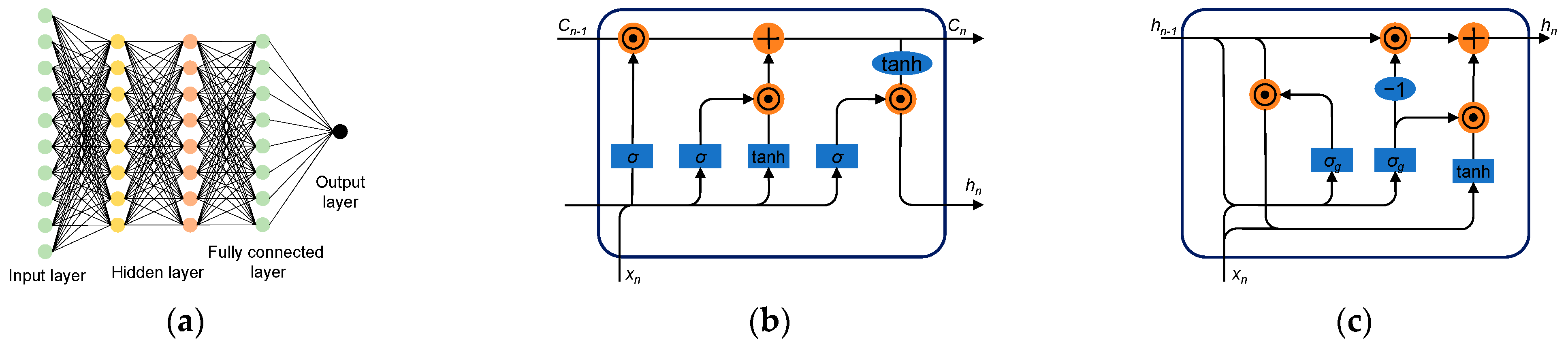
3.1. Recurrent Neural Network

The real-time prognostics of PEMFC performance degradation induced by the operating conditions forms a time-series prediction problem. Currently, there are many data-driven methods can handle such problems, including regression-based methods and neural networks. The PEMFC performance degradation is a long-term evolution process. The RNNs cannot handle the long-term dependencies effectively. Thus, this study used two extended versions of RNN, LSTM, and GRU (shown in Figure 5), to predict PEMFC performance. The hidden layer could be configured as using either LSTM or GRU.

3.1.1. Basics of LSTM

The forget gate of LSTM (f_n) decides to preserve or remove what part of last hidden states (h_n−1) via a sigmoid function (σ_g) based on the last hidden states (h_n−1) and current input (x_n),

$$f_n={\sigma }_g\left(W_{fx}{x}_n+b_f+W_{fh}{h}_{n-1}\right),$$

(32)

where W, R, and b are the input weight matrices, recurrent weight matrices, and bias of forget gate, respectively, and σ_g is the sigmoid activation function. The input gate decides what part of the new information can be added to the current cell state (C_n),

$$C_n=f_n\odot C_{n-1}+i_n\odot C_n^{’},$$

(33)

where i_n is the updated values and $C_n^{’}$ represents the candidate values that will be added to the cell state,

$$\left\{\begin{array}{l}{i}_n={\sigma }_g\left(W_{ix}{x}_n+b_i+W_{ih}{h}_{n-1}\right)\\ C_n^{’}={\sigma }_s\left(W_{ix}{x}_n+b_i+W_{ih}{h}_{n-1}\right)\end{array}\right.,$$

(34)

where σ_s is the tanh activation function. The output gate decides what part of the current cell state (C_n) contributes.

$$V_{error}=\sqrt{{\displaystyle \frac{{\displaystyle \sum \left(V_{cell}-V_{polar,exp}\right)}}{m}}},$$

(35)

3.1.2. Basics of GRU

GRU is an extended version of LSTM. It uses only two gates, i.e., the reset gate and update gate. The reset gate (r_n) selectively forgets the last time steps hidden state (h_n−1). The update gate (z_n) selectively passes the previous time steps hidden state.

$$\left\{\begin{array}{l}{r}_n={\sigma }_g\left(W_r{x}_n+b_r+R_r{h}_{n-1}\right)\\ z_n={\sigma }_g\left(W_z{x}_n+b_r+R_z{h}_{n-1}\right)\end{array}\right.,$$

(36)

The hidden state (h_n) can be calculated by the hidden state of the candidate and the last time step.

$$\left\{\begin{array}{l}{\tilde{h}}_n={\sigma }_s\left(W_{\tilde{h}}{x}_n+b_{w_{\tilde{h}}}+r_n\odot \left(R_{\tilde{h}}{h}_{n-1}\right)\right)\\ h_n=\left(1-z_n\right)\odot {\tilde{h}}_n+z_n\odot h_{n-1}\end{array}\right.,$$

(37)

3.2. Dataset Analysis and Screening

The operating conditions, such as anode and cathode pressure, relative humidity at anode and cathode inlet, flow rate of hydrogen and air, and temperature of inlet and outlet of both electrodes, are highly related to the performance degradation. Many research only take the previous voltage as input, which did not count the operating conditions influence. Using all the recorded data as the input can increase the complexity and computational load of the prediction model. Data analysis, such as analyzing and uncovering the most contribution components, is necessary to balance the complexity and accuracy of data-driven prediction. Therefore, this section screens the most sensible data to reduce the input data dimension. In this study, the fuel cell output voltage is the direct indictor to measure the PEMFC performance. The recorded operational data, including pressure and temperature at the inlet and outlet ports of both anode and cathode, flow rate of hydrogen and air, current density, and the experiment voltage, are screened.

While semi-empirical model exhibits inherent limitations in predicting voltage diminution induced by performance degradation (as shown in Figure 3), they demonstrate notable competency in resolving voltage transients attributable to operational condition perturbations. With the help of the highly computationally efficient semi-empirical model, data-driven methods may be able to reduce complexity while ensuring identical prediction accuracy. Therefore, this research combines the semi-empirical model output and the twelve recorded operating data to screen the most sensible parameters.

Correlation analysis methods, including Pearson and Spearman methods, are the practical statistical measures for data analysis and screening. This study calculated the Pearson correlation coefficients, and the results are illustrated in Figure 6. The current density (curr den), semi-empirical model output (V_sm), pressure at inlet and outlet ports of the cathode (P_ca,in and P_ca,out), the inlet temperature of hydrogen and air (T_H,in and T_air,in), and the flow rate of hydrogen and air (f_lowair,in and f_lowh,in) are highly relevant to the experiment voltage, since their correlation coefficients are larger than 0.3. Hence, the training dataset comprises those eight parameters and the experiment voltage.

3.3. Method Development and Training

According to the dataset analysis and screening, seven operating-related datapoints are collected and fed to the developed RNN. The semi-empirical model, with its calculated voltage as part of input features, constitutes the model information involved in the RNN. Additionally, the experiment voltage from the previous step composes the input features, as shown in Figure 7.

In real-time fuel cell degradation predictions, the sliding window methodology to process temporal operational data is implemented. The predictive framework utilizes measurements from preceding window intervals (10 time steps in this study), comprising the key parameters rigorously screened in Section 3.2, as inputs to forecast the present-step output voltage (V_pred). Conventional approaches typically assume complete ignorance of current-step parameters; however, in the PEMFC health-aware fuel cell vehicle energy management strategy, optimal power allocation is achieved through health-constrained cost function minimization derived from controller-demanded current profiles. To reconcile this operational paradigm, the proposed architecture uniquely treats the present-step current demand (I_n) as a known input during voltage prediction. Furthermore, acknowledging dynamic variations in operating conditions (e.g., temperature and pressure) during transient operation, where real-time monitoring exhibits inherent latency, the nominal operating conditions (specified in Table 1) are employed as baseline inputs to the semi-empirical model, thereby generating reference voltage outputs (V_sm) through first-principles-informed empirical computations. Therefore, the thorough prediction process in this study can be given in Equation (38),

$$V_{pred,n}=f\left(F_{n-10},\dots ,F_{n-1},I_n,V_{sm,n}\right)$$

(38)

where F is the input features screened in Section 3.2. and f is the prediction function. The 1000 h testing dataset is split into a training set and testing set, where the data from 0 to 250 h are the training set and the data from 250 to 1000 h are the testing set. To compare the efficacy of the proposed model, a comprehensive benchmarking campaign was conducted using conventional RNN methodology implemented on identical neural architecture. and the input features except the semi-empirical model voltage. The neural network architecture implemented in this study comprises an input layer, hidden neuron layers with corresponding activation functions, dropout regularization layers, fully connected (dense) layers, and a regression output layer. The layer-specific architectural parameters are systematically tabulated in

Table 4. Summary of neural network details.

RNN Architecture	Layer Parameters	Model Involved RNN	RNN
Input layer	Number of features	9	8
Hidden layer	Number of neurons	32/48/64	32/48/64
Dropout layer	Probability	0.5	0.5
Fully connect layer	Number of neurons	32/48/64	32/48/64
Regression layer	Number of outputs	1	1

. All the RNNs share the identical training details, as shown in

Table 5. Training details of neural network.

Training Parameters	Values
Max Epochs	500
Mini Batch Size	4096
Learning rate	0.005
Learning rate drop factor	0.2
Learning rate drop period	50

.

4. Discussion

Using 25% of the total 1000 h dataset as training data, the proposed methods and traditional RNNs are trained and the prediction performance measured by RMSE is summarized in

Table 6. Summary of different prediction methods’ performance (measured by RMSE).

Number of Neurons	Model Involved RNN		RNN
	LSTM	GRU	LSTM	GRU
32	0.6973	0.6985	0.7120	0.7113
48	0.6446	0.6444	0.6632	0.6622
64	0.6228	0.6229	0.6421	0.6422

. The maximum RMSE is only 0.7120%, validating that all methods can accurately predict the PEMFC performance degradation. Without the assistance of the semi-empirical model, the best indicator that RNN methods can achieve is 0.6421%. Even though the current density is highly correlated with the PEMFC voltage, it is difficult to predict the voltage of PEMFC based on the previous features and the current demand, especially when the PEMFC has been degraded. The neural networks must learn the voltage fluctuations mechanism brought by both current changing and degradation. This complexity requires a larger number of neurons and/or layers, which can explain why the performance indicator in Table 6 descends along with the increasing number of neurons. Nevertheless, more neurons and layers does not necessarily mean better; the number of neurons and layers in the neural network need to be optimized to fit the scale of the training dataset and the complexity of problem [46].

The presence of V_sm gives a reference voltage value under current demand, which can demote the current changing influences. The learning algorithm can focus on the degradation mechanism. With the same RNN configurations, the model-involved RNN can improve the prediction performance compared to the RNN methods without semi-empirical model information. The average improvement can reach 2.56%, the maximum improvement can be up to 3.01%. Figure 8 exhibits the predicted voltage. The model-involved method can predict the PEMFC performance very well through the lifecycle. At BoL, the RMSE of prediction and experiment voltage is 0.3272%. the maximum absolute error reduces is 0.0217 V. After 836 h testing, the prediction accuracy of model-involved method can be maintained at 0.5631% (measured by RMSE), and the maximum absolute voltage error is only 0.0471 V. In addition, the model-involved RNN can reach a comparable prediction performance using a smaller number of neurons. For instance, the prediction performance of model-involved LSTM (48 neurons) is 0.6446%, while the performance indicator of LSTM methods (64 neurons) without model information is 0.6421%. The computational load can be lowered thanks to the lightweight RNN, which can be implemented in a real-time controller easily. Furthermore, there is no obvious difference between LSTM and GRU.

To further validate the efficacy of proposed model-involved method, more cases using different training dataset scales are attempted. The prediction performance is depicted in Figure 9. When the training dataset scale is cut down to 15% of the total dataset, the prediction performance of model-involved LSTM slightly decreases. The prediction RMSE of using a different number of neurons is 0.7630%, 0.7057%, and 0.6784%, respectively. The prediction performance is decreased by 9.42%, 9.48%, and 8.93%, compared to using 25% of the dataset for training. However, if the training dataset is downsized to 5% of the total dataset, the prediction performance significantly decreases. The prediction error, measured by RMSE, increased to 1.3565%, 1.2411%, and 1.1922%, which almost doubles the prediction performance of that using 25% training dataset. The smaller training error of using 5% of the dataset suggests the possibility of overfitting.

5. Conclusions

This study proposes a hybrid prognostics framework integrating semi-empirical electrochemical modeling with recurrent neural networks to predict voltage decay trajectories in proton exchange membrane fuel cells. The methodology advances existing approaches through three innovations:

• Mechanistically grounded model reformulation: The semi-empirical framework was rederived from first principles, explicitly incorporating Nernstian potential dynamics and mass transport limitations during redox reactions.
• Intelligent parameter identification: Critical model coefficients were optimized via a grey wolf optimization algorithm with adaptive convergence thresholds, calibrated against experimental polarization data.
• Physics-informed data fusion: Voltage predictions from the calibrated model were concatenated with operational boundary conditions (current density, temperature, humidity) to generate hybrid training datasets, which underwent rigorous statistical screening via cross-correlation analysis to eliminate multicollinear features.

A bidirectional RNN architecture was subsequently trained on the curated dataset to capture both forward and backward temporal dependencies in degradation patterns. The experimental validation revealed two critical insights. (1) Enhanced prognostic fidelity: Integration of semi-empirical voltage baselines reduced RNN prediction error by 3.01% compared to purely data-driven approaches, as quantified through root mean square error. Pearson correlation coefficient analysis confirmed that model-derived voltage residuals (deviation from ideal electrochemical behavior) constituted the most degradation-sensitive input feature. (2) Operational resilience: The hybrid framework demonstrated superior data efficiency, achieving comparable accuracy to conventional methods with 35% less training data—a critical advantage for real-world deployment where comprehensive degradation datasets are often unavailable. However, given the current scarcity of comprehensive durability datasets across PEMFC architectures, particularly those encompassing full lifecycle operational extremes, the proposed methodology’s generalizability has not yet been extended to alternative PEMFC topologies with divergent material compositions or flow field geometries.

References

1. Lagioia, G.; Spinelli, M.P.; Amicarelli, V. Blue and Green Hydrogen Energy to Meet European Union Decarbonisation Objectives. An Overview of Perspectives and the Current State of Affairs. Int. J. Hydrogen Energy 2022, 48, 1304–1322. [Google Scholar] [CrossRef]
2. Dirkes, S.; Leidig, J.; Fisch, P.; Pischinger, S. Prescriptive Lifetime Management for PEM Fuel Cell Systems in Transportation Applications, Part I: State of the Art and Conceptual Design. Energy Convers. Manag. 2023, 277, 116598. [Google Scholar] [CrossRef]
3. Feng, Y.; Liu, Q.; Li, Y.; Yang, J.; Dong, Z. Energy Efficiency and CO2 Emission Comparison of Alternative Powertrain Solutions for Mining Haul Truck Using Integrated Design and Control Optimization. J. Clean. Prod. 2022, 370, 133568. [Google Scholar] [CrossRef]
4. Feng, Y.; Dong, Z. Comparative Lifecycle Costs and Emissions of Electrified Powertrains for Light-Duty Logistics Trucks. Transp. Res. Part D Transp. Environ. 2023, 117, 103672. [Google Scholar] [CrossRef]
5. Ren, P.; Pei, P.; Li, Y.; Wu, Z.; Chen, D.; Huang, S. Degradation Mechanisms of Proton Exchange Membrane Fuel Cell under Typical Automotive Operating Conditions. Prog. Energy Combust. Sci. 2020, 80, 100859. [Google Scholar] [CrossRef]
6. Zhang, T.; Wang, P.; Chen, H.; Pei, P. A Review of Automotive Proton Exchange Membrane Fuel Cell Degradation under Start-Stop Operating Condition. Appl. Energy 2018, 223, 249–262. [Google Scholar] [CrossRef]
7. Chen, H.; Pei, P.; Song, M. Lifetime Prediction and the Economic Lifetime of Proton Exchange Membrane Fuel Cells. Appl. Energy 2015, 142, 154–163. [Google Scholar] [CrossRef]
8. Ma, R.; Chai, X.; Geng, R.; Xu, L.; Xie, R.; Zhou, Y.; Wang, Y.; Li, Q.; Jiao, K.; Gao, F. Recent Progress and Challenges of Multi-Stack Fuel Cell Systems: Fault Detection and Reconfiguration, Energy Management Strategies, and Applications. Energy Convers. Manag. 2023, 285, 117015. [Google Scholar] [CrossRef]
9. Borup, R.; Meyers, J.; Pivovar, B.; Kim, Y.S.; Mukundan, R.; Garland, N.; Myers, D.; Wilson, M.; Garzon, F.; Wood, D.; et al. Scientific Aspects of Polymer Electrolyte Fuel Cell Durability and Degradation. Chem. Rev. 2007, 107, 3904–3951. [Google Scholar] [CrossRef]
10. Tarasevich, M.R.; Korchagin, O.V. Rapid diagnostics of characteristics and stability of fuel cells with proton-conducting electrolyte. Russ. J. Electrochem. 2014, 50, 737–750. [Google Scholar] [CrossRef]
11. Avakov, V.B.; Bogdanovskaya, V.A.; Kapustin, A.V.; Korchagin, O.V.; Kuzov, A.V.; Landgraf, I.K.; Stankevich, M.M.; Tarasevich, M.R. Lifetime prediction for the hydrogen–air fuel cells. Russ. J. Electrochem. 2014, 51, 570–586. [Google Scholar] [CrossRef]
12. Pei, P.; Chen, D.; Wu, Z.; Ren, P. Nonlinear Methods for Evaluating and Online Predicting the Lifetime of Fuel Cells. Appl. Energy 2019, 254, 113730. [Google Scholar] [CrossRef]
13. Bressel, M.; Hilairet, M.; Hissel, D.; Bouamama, B.O. Extended Kalman Filter for Prognostic of Proton Exchange Membrane Fuel Cell. Appl. Energy 2016, 164, 220–227. [Google Scholar] [CrossRef]
14. Jouin, M.; Bressel, M.; Morando, S.; Gouriveau, R.; Hissel, D.; Péra, M.-C.; Zerhouni, N.; Jemei, S.; Hilairet, M.; Bouamama, B.O. Estimating the End-of-Life of PEM Fuel Cells: Guidelines and Metrics. Appl. Energy 2016, 177, 87–97. [Google Scholar] [CrossRef]
15. Lo, J.; Hu, Z.; Xu, L.; Ouyang, M.; Fang, C.; Hu, J.; Cheng, S.; Hong, P.; Zhang, W.; Jiang, H. Fuel Cell System Degradation Analysis of a Chinese Plug-in Hybrid Fuel Cell City Bus. Int. J. Hydrogen Energy 2016, 41, 15295–15310. [Google Scholar] [CrossRef]
16. Hu, Z.; Xu, L.; Li, J.; Ouyang, M.; Song, Z.; Huang, H. A Reconstructed Fuel Cell Life-Prediction Model for a Fuel Cell Hybrid City Bus. Energy Convers. Manag. 2018, 156, 723–732. [Google Scholar] [CrossRef]
17. Hua, Z.; Zheng, Z.; Pahon, E.; Péra, M.-C.; Gao, F. A Review on Lifetime Prediction of Proton Exchange Membrane Fuel Cells System. J. Power Sources 2022, 529, 231256. [Google Scholar] [CrossRef]
18. Cheng, Y.; Zerhouni, N.; Lu, C. A Hybrid Remaining Useful Life Prognostic Method for Proton Exchange Membrane Fuel Cell. Int. J. Hydrogen Energy 2018, 43, 12314–12327. [Google Scholar] [CrossRef]
19. Ma, R.; Yang, T.; Breaz, E.; Li, Z.; Briois, P.; Gao, F. Data-Driven Proton Exchange Membrane Fuel Cell Degradation Predication through Deep Learning Method. Appl. Energy 2018, 231, 102–115. [Google Scholar] [CrossRef]
20. Liu, H.; Chen, J.; Hissel, D.; Su, H. Remaining useful life estimation for proton exchange membrane fuel cells using a hybrid method. Appl. Energy 2019, 237, 910–919. [Google Scholar] [CrossRef]
21. Zuo, J.; Lv, H.; Zhou, D.; Xue, Q.; Jin, L.; Zhou, W.; Yang, D.; Zhang, C. Deep Learning Based Prognostic Framework towards Proton Exchange Membrane Fuel Cell for Automotive Application. Appl. Energy 2021, 281, 115937. [Google Scholar] [CrossRef]
22. Yue, M.; Li, Z.; Roche, R.; Jemei, S.; Zerhouni, N. Degradation Identification and Prognostics of Proton Exchange Membrane Fuel Cell under Dynamic Load. Control Eng. Pract. 2022, 118, 104959. [Google Scholar] [CrossRef]
23. Zhang, S.; Chen, T.; Xiao, F.; Zhang, R. Degradation prediction model of PEMFC based on multi-reservoir echo state network with Mini Reservoir. Int. J. Hydrogen Energy 2022, 47, 40026–40040. [Google Scholar] [CrossRef]
24. Long, B.; Wu, K.; Li, P.; Li, M. A Novel Remaining Useful Life Prediction Method for Hydrogen Fuel Cells Based on the Gated Recurrent Unit Neural Network. Appl. Sci. 2022, 12, 432. [Google Scholar] [CrossRef]
25. Tao, Z.; Zhang, C.; Xiong, J.; Hu, H.; Ji, J.; Peng, T.; Nazir, M.S. Evolutionary gate recurrent unit coupling convolutional neural network and improved manta ray foraging optimization algorithm for performance degradation prediction of PEMFC. Appl. Energy 2023, 336, 120821. [Google Scholar] [CrossRef]
26. Zhang, R.; Chen, T.; Xiao, F.; Luo, J. Bi-Directional Gated Recurrent Unit Recurrent Neural Networks for Failure Prognosis of Proton Exchange Membrane Fuel Cells. Int. J. Hydrogen Energy 2022, 47, 33027–33038. [Google Scholar] [CrossRef]
27. Hua, Z.; Yang, Q.; Chen, J.; Lan, T.; Zhao, D.; Dou, M.; Liang, B. Degradation prediction of PEMFC based on BiTCN-BiGRU-ELM fusion prognostic method. Int. J. Hydrogen Energy 2024, 87, 361–372. [Google Scholar] [CrossRef]
28. Li, S.; Luan, W.; Wang, C.; Chen, Y.; Zhuang, Z. Degradation Prediction of Proton Exchange Membrane Fuel Cell Based on Bi-LSTM-GRU and ESN Fusion Prognostic Framework. Int. J. Hydrogen Energy 2022, 47, 33466–33478. [Google Scholar] [CrossRef]
29. Yakut, Y.B. Short-term voltage loss prediction in PEMFCs using single-step and multi-step LSTM models. Int. J. Hydrogen Energy 2025. [Google Scholar] [CrossRef]
30. Huang, R.; Zhang, X.; Dong, S.; Huang, L.; Li, Y. Degradation prediction of PEM fuel cell using LSTM based on Gini gamma correlation coefficient and improved sand cat swarm optimization under dynamic operating conditions. Appl. Energy 2025, 392, 125967. [Google Scholar] [CrossRef]
31. Yang, J.; Chen, L.; Zhang, B.; Zhang, H.; Chen, B.; Wu, X.; Deng, P.; Xu, X. Remaining useful life prediction for vehicle-oriented PEMFCs based on organic gray neural network considering the influence of dual energy source synergy. Energy 2025, 322, 135578. [Google Scholar] [CrossRef]
32. Liu, Y.; Li, H.; Yang, Y.; Zhu, W.; Xie, C.; Yu, X.; Guo, B. Reliability assessment of PEMFC aging prediction based on probabilistic Bayesian mixed recurrent neural networks. Renew. Energy 2025, 246, 122892. [Google Scholar] [CrossRef]
33. Wang, F.-K.; Cheng, F.K.X.-B.; Hsiao, K.-C. Stacked Long Short-Term Memory Model for Proton Exchange Membrane Fuel Cell Systems Degradation. J. Power Sources 2020, 448, 227591. [Google Scholar] [CrossRef]
34. Zuo, J.; Lv, H.; Zhou, D.; Xue, Q.; Jin, L.; Zhou, W.; Yang, D.; Zhang, C. Long-Term Dynamic Durability Test Datasets for Single Proton Exchange Membrane Fuel Cell. Data Brief 2021, 35, 106775. [Google Scholar] [CrossRef]
35. Wilberforce, T.; Alaswad, A.; Garcia–Perez, A.; Xu, Y.; Ma, X.; Panchev, C. Remaining Useful Life Prediction for Proton Exchange Membrane Fuel Cells Using Combined Convolutional Neural Network and Recurrent Neural Network. Int. J. Hydrogen Energy 2022, 48, 291–303. [Google Scholar] [CrossRef]
36. Wang, Y.; Wu, K.; Zhao, H.; Li, J.; Sheng, X.; Yin, Y.; Du, Q.; Zu, B.; Han, L.; Jiao, K. Degradation Prediction of Proton Exchange Membrane Fuel Cell Stack Using Semi-Empirical and Data-Driven Methods. Energy AI 2022, 11, 100205. [Google Scholar] [CrossRef]
37. Wu, K.; Du, Q.; Zu, B.; Wang, Y.; Cai, J.; Gu, X.; Xuan, J.; Jiao, K. Enabling Real-Time Optimization of Dynamic Processes of Proton Exchange Membrane Fuel Cell: Data-Driven Approach with Semi-Recurrent Sliding Window Method. Appl. Energy 2021, 303, 117659. [Google Scholar] [CrossRef]
38. Liu, Z.; Sun, H.; Xu, L.; Mao, L.; Hu, Z.; Li, J. Toward low-data and real-time PEMFC diagnostic: Multi-sine stimulation and hybrid ECM-informed neural network. Appl. Energy 2025, 391, 125959. [Google Scholar] [CrossRef]
39. Ko, T.; Kim, D.; Park, J.; Lee, S.H. Physics-informed neural network for long-term prognostics of proton exchange membrane fuel cells. Appl. Energy 2025, 382, 125318. [Google Scholar] [CrossRef]
40. Yuan, Y.; Qu, Z.; Wang, W.; Ren, G.; Hu, B. Illustrative Case Study on the Performance and Optimization of Proton Exchange Membrane Fuel Cell. ChemEngineering 2019, 3, 23. [Google Scholar] [CrossRef]
41. Mirjalili, S.; Mirjalili, S.M.; Lewis, A. Grey Wolf Optimizer. Adv. Eng. Softw. 2019, 69, 46–61. [Google Scholar] [CrossRef]
42. Jouin, M.; Gouriveau, R.; Hissel, D.; Péra, M.-C.; Zerhouni, N. Degradations Analysis and Aging Modeling for Health Assessment and Prognostics of PEMFC. Reliab. Eng. Syst. Saf. 2016, 148, 78–95. [Google Scholar] [CrossRef]
43. Jao, T.-C.; Jung, G.-B.; Kuo, S.-C.; Tzeng, W.-J.; Su, A. Degradation Mechanism Study of PTFE/Nafion Membrane in MEA Utilizing an Accelerated Degradation Technique. Int. J. Hydrogen Energy 2012, 37, 13623–13630. [Google Scholar] [CrossRef]
44. Collette, F.; Thominette, F.; Mendil-Jakani, H.; Gebel, G. Structure and Transport Properties of Solution-Cast Nafion® Membranes Subjected to Hygrothermal Aging. J. Membr. Sci. 2013, 435, 242–252. [Google Scholar] [CrossRef]
45. Hong, J.; Yang, H.; Liang, F.; Li, K.; Zhang, X.; Zhang, H.; Zhang, C.; Yang, Q.; Wang, J. State of Health Prediction for Proton Exchange Membrane Fuel Cells Combining Semi-Empirical Model and Machine Learning. Energy 2024, 291, 130364. [Google Scholar] [CrossRef]
46. Hongwei, L.; Binxin, Q.; Zhicheng, H.; Junnan, L.; Yue, Y.; Guolong, L. An Interpretable Data-Driven Method for Degradation Prediction of Proton Exchange Membrane Fuel Cells Based on Temporal Fusion Transformer and Covariates. Int. J. Hydrogen Energy 2023, 48, 25958–25971. [Google Scholar] [CrossRef]
Figure 1. A general schematic of a PEMFC architecture [40].
Energies 18 02665 g001
Figure 2. Precise semi-empirical model performance at BoL.
Energies 18 02665 g002
Figure 3. Semi-empirical model prediction performance: (a) at BoL; (b) after 836 h test.
Energies 18 02665 g003
Figure 4. Fitted parameters varying along with PEMFC degradation testing: (a) fGDL,an; (b) fGDL,ca; (c) ileak,an; (d) ileak,ca.
Energies 18 02665 g004
Figure 5. Data-driven prediction model: (a) model architecture; (b) LSTM structure; (c) GRU structure.
Energies 18 02665 g005
Figure 6. Pearson correlation coefficients results.
Energies 18 02665 g006
Figure 7. Schematic of model involve architecture integration in RNN frameworks.
Energies 18 02665 g007
Figure 8. Predicted results comparison using 25% of the dataset: (a) at BoL; (b) after 836 h test.
Energies 18 02665 g008
Figure 9. Predicted performance comparison of the model-involved LSTM method.
Energies 18 02665 g009