Article

Evaluation and Bias Correction of the ERA5 Reanalysis over the United States for Wind and Solar Energy Applications

by
James M. Wilczak
1,*,
Elena Akish
1,2,
Antonietta Capotondi
1,2 and
Gilbert P. Compo
1,2
1
NOAA Physical Sciences Laboratory, Boulder, CO 80305, USA
2
Cooperative Institute for Research in Environmental Sciences (CIRES), University of Colorado, Boulder, CO 80309, USA
*
Author to whom correspondence should be addressed.
Energies 2024, 17(7), 1667; https://doi.org/10.3390/en17071667
Submission received: 17 February 2024 / Revised: 22 March 2024 / Accepted: 26 March 2024 / Published: 31 March 2024
(This article belongs to the Special Issue The Application of Weather and Climate Research in the Energy Sector)

Abstract

:
The applicability of the ERA5 reanalysis for estimating wind and solar energy generation over the contiguous United States is evaluated using wind speed and irradiance variables from multiple observational data sets. After converting ERA5 and observed meteorological variables into wind power and solar power, comparisons demonstrate that significant errors in the ERA5 reanalysis exist that limit its direct applicability for a wind and solar energy analysis. Overall, ERA5-derived solar power is biased high, while ERA5-derived wind power is biased low. During winter, the ERA5-derived solar power is biased high by 23% on average, while on an annual basis, the ERA5-derived wind power is biased low by 20%. ERA5-derived solar power errors are found to have consistent characteristics across the contiguous United States. Errors for the shortest duration and most extreme solar negative anomaly events are relatively small in the ERA5 when completely overcast conditions occur in both the ERA5 and observations. However, longer-duration anomaly events on weekly to monthly timescales, which include partially cloudy days or a mix of cloudy and sunny days, have significant ERA5 errors. At 10 days duration, the ERA5-derived average solar power produced during the largest negative anomaly events is 62% greater than observed. The ERA5 wind speed and derived wind power negative biases are largely consistent across the central and northwestern U.S., and offshore, while the northeastern U.S. has an overall small net bias. For the ERA5-derived most extreme negative anomaly wind power events, at some sites at 10 days duration, the ERA5-derived wind power produced can be less than half of that observed. Corrections to ERA5 are derived using a quantile–quantile method for solar power and linear regression of wind speed for wind power. These methods are shown to avoid potential over-inflation of the reanalysis variability resulting from differences between point measurements and the temporally and spatially smoother reanalysis values. The corrections greatly reduce the ERA5 errors, including those for extreme events associated with wind and solar energy droughts, which will be most challenging for electric grid operation.

1. Introduction

Accurate meteorological data sets will be essential for planning the development of a future energy system that includes large amounts of wind and solar energy. Gridded data sets will be needed that cover all geographic areas where wind and solar generation will be developed, and that span many decades in order to include the full range of meteorology that can occur, including rare extreme events that would cause the greatest stress on the electric grid system.
In a recent overview of meteorological requirements for energy system planning, Sharp [1] emphasizes that, for energy system planning purposes, these wind and solar data sets should be dynamically consistent and be thoroughly validated in the region where they will be applied by calibrating them against observations and applying corrections if needed. For solar, gridded data sets derived from combining visible satellite imagery with radiative transfer models are now commonly used, as well as conventional reanalysis products. For wind energy, only NWP-based reanalysis products are available. Reanalysis products offer dynamically consistent wind and solar energy estimates, and among the various global reanalysis data available, the ERA5 has been found to be the most accurate for hub-height winds in a review by Gualtieri [2] and for wind and solar irradiances in the work by Kies et al. [3], primarily using observations from Europe. In the present analysis, extensive wind and solar irradiance observational data sets are used first to evaluate the ERA5 reanalysis over the contiguous United States (CONUS) and then to correct systematic errors found in the ERA5 using standard correction techniques.
Among the studies that have evaluated ERA5 hub-height wind speeds against observations, the most comprehensive is the analysis from Dörenkämper et al. [4], who used wind speed observations from 291 tall towers across Europe. They found that the ERA5 underestimates the wind speed, with a negative bias of ~1.5 ms−1, resulting in a mean wind power bias of −40%, with the bias increasing in magnitude in regions with more complex terrain. Jourdier [5] used a smaller set of 7 tall towers and 1 lidar located in France, finding a negative ERA5 bias of −0.5 ms−1 in flat terrain, which increased to −1.7 ms−1 in areas of more complex terrain, and did not find any consistent diurnal variation. Similarly, Gualtieri [6] compared ERA5 wind speeds to observations from 6 tall towers and found that, on average, the ERA5 underestimated the observed speeds. In a comparison of the ERA5 with hub-height wind speed observations at 14 sites in Europe, Brune et al. [7] found significant variation in the bias between sites, with small but negative biases of −0.2 ms−1 over water and in areas of complex terrain, but a near-zero bias in flat terrain. In North America, Pronk et al. [8] evaluated the ERA5 using one year of data from one lidar in the central U.S., and offshore near New Jersey using two floating lidars. In both the onshore and offshore locations, the ERA5 had large negative biases (−1.5 ms−1 and −0.8 ms−1, respectively), which were both diurnally and seasonally independent. Sheridan et al. [9] evaluated the ERA5 against two floating lidars off of Virginia, finding a negative ERA5 bias, although effects of the nearby coast may have impacted one of the sites. Sheridan et al. [10] also evaluated the ERA5 against two floating lidars off of California, finding a negative bias of −0.4 ms−1 for the lidar that had a complete year of data. Overall, these results indicate that the ERA5 tends to underestimate observed hub-height wind speeds, with the magnitude of the bias increasing in regions of more complex terrain, and with the bias independent of time of day and season.
Multiple studies have also evaluated ERA5 solar radiation variables using in situ observations. Most commonly, the downward shortwave radiation on a horizontal surface has been the variable evaluated [11,12,13,14,15,16]. These studies all find that, on a yearly average basis, the ERA5 has a 5–20 Wm−2 high bias, while some [11,16] also have demonstrated that the positive bias is larger for cloudy conditions. Fewer studies have evaluated the solar direct and diffuse components of downward solar irradiance, which are required for calculating solar power on tilted panels. Using a network of 17 stations in China, Wu et al. [17] found that the ERA5 underestimates the diffuse irradiance, while Jiang et al. [18], using an observation network of 39 stations in China, found that the ERA5 underestimates diffuse radiation by 43 Wm−2, but overestimates the direct radiation by 74 Wm−2. Using observations from 14 stations, Li et al. [19] also found a negative ERA5 bias for diffuse irradiance, and a positive bias for the direct beam, and concluded that, in addition to cloud effects, at least part of these biases can be attributed to aerosols. Finally, Mathews et al. [20] demonstrate that, if uncorrected, the solar irradiance errors in reanalysis data sets, including the ERA5, can lead to distortions in the total energy requirement of long-duration energy storage infrastructure in grid planning studies.
In the present analysis, the evaluation and calibration of the ERA5 is based on daily averages of ERA5 wind speed and ERA5-derived solar power. Using daily averaged values reduces scale mismatch effects that can arise between the comparison of high temporal resolution point measurements with temporally and spatially smoother variables [21]. However, for wind power, the calibration of the ERA5 is then applied to hourly values of wind speed, while for solar power the corrections based on daily averages can also be applied to ERA5-derived values at an hourly timescale, if desired. These issues are discussed in more detail in Section 4.3 and Section 5.2.
The outline of this manuscript is as follows. Section 2 describes the data sets used. Section 3 describes the methods used for converting wind speed and solar irradiances to wind and solar power. Section 4 evaluates the accuracy of ERA5 solar irradiances and ERA5-derived solar power, and then corrects the power using a quantile–quantile-based method. Section 5 evaluates the accuracy of ERA5 wind speeds and ERA5-derived wind power, and then corrects the wind speeds using linear regression. Finally, Section 6 provides a summary and additional discussion of the results. The novel aspects of this study are that (1) it quantifies both ERA5-derived wind and solar energy errors across the CONUS; (2) it demonstrates that corrections applied to daily ERA5-based values also improve the accuracy of the most extreme negative anomaly values across a range of time scales from weeks to months, which would be important for wind and solar energy drought analyses; and (3) it demonstrates that the correction methods used do not result in any significant over-inflation of the variability of the ERA5-derived values resulting from correcting model grid cell values with hourly sampled point measurements.

2. Data Sets

Observational data sets are used to quantify the accuracy of ERA5 reanalysis fields for renewable energy applications and to develop corrections to improve estimates of wind and solar energy generation derived from the ERA5. For solar, the observations include the NOAA Surface Radiation budget (SURFRAD) and Solar Radiation (SOLRAD) networks, and the DOE Atmospheric Radiation Measurement Southern Great Plains (ARM-SGP) array of solar irradiance observations. The DOE National Solar Radiation Database (NSRDB) data set is also used to validate some of the assumptions made in correcting the ERA5-derived solar power. For winds, we use observations of near turbine-height winds from the first and second Wind Forecast Improvement Projects (WFIP1 and WFIP2), the New York Mesonet, the DOE ARM-SGP lidar array, New York State Energy Research and Development (NYSERDA) and DOE offshore buoy-mounted lidars, and individual towers or lidars in several other locations. Each of these data sets is described in detail below.

2.1. ERA5

Meteorological reanalyses such as the ERA5 [22] provide continuous reconstructions of past weather conditions by objectively combining a global weather prediction model forecast with observations while accounting for uncertainty in both the forecast and the observations. The ERA5 reanalysis, based on the ECMWF IFS model, has a native horizontal resolution of ~31 km and is provided on a uniform 0.25 degree grid. Variables used in this analysis include instantaneous hourly values of the 100 m zonal (U) and meridional (V) wind components, 2 m temperature, 10 m horizontal wind speed, and surface pressure, together with hourly accumulated solar direct beam irradiance on a horizontal plane (DIRhor), diffuse irradiance on a horizontal plane (DHI), and global horizontal irradiance (GHI). Because of limitations in the model’s physical parameterization schemes and grid resolution, biases can occur in any of the reanalysis variables.

2.2. Solar Observations

The combined NOAA SURFRAD and SOLRAD network [23,24] comprises 14 stations that span the CONUS (Figure 1). For the time period analyzed (1998–2020), the network measured GHI, direct normal incident (DNI), and diffuse on a horizontal surface (DHI) irradiances, in addition to surface albedo, temperature, and wind speed. Because of routine blockage of the radiation sensors for some hours of the day, the Hanford, CA SOLRAD site was excluded.
The DOE ARM-SGP radiation network (Figure 1) spans an approximately 370 km N-S by 330 km E-W area in north-central Oklahoma and southern Kansas. In the calculation of solar power, observations of DNI, DHI, and GHI [25], as well as surface albedo, temperature, and wind speed, were used for the period of 1998–2020. During the entire period, there were 28 unique sites. However, as some sites were discontinued while new sites were established, the greatest number of sites potentially available at any one time was 23, and the minimum number was 13. The typical spacing between sites of the latest and densest configuration of stations was approximately 20 km, so each site corresponds approximately to a unique ERA5 grid cell.
A potential challenge with using solar observational data sets for solar drought evaluation is that spurious results could occur if extreme care is not taken to keep the instrument domes clean and to avoid the effects of snow, frost, or rain on the measurements. The ARM-SGP and SURFRAD/SOLRAD stations were used in this study because of their rigorous maintenance, frequent calibration regimens, and careful quality assurance. In addition, the instruments are ventilated or kept heated at a high temperature to eliminate the effects of rain, dew, frost, and snow [23]. The overall accuracy for the DNI measurements is 2–3% [24] and for DHI it is ±0.5% [26]. We also note that surface radiation measurements are an independent data set that can be used to evaluate the ERA5, as the ERA5 does not assimilate any of these observations.

2.3. Wind Observations

As for solar, only wind observations (from lidar, sodar, or in situ anemometers on tall towers) with well-defined maintenance/calibration regimes were used, and, in addition, it was required that at least one full year of data was available for each location. For tower data, we required booms on different sides of the towers to avoid tower shadowing effects, the identification of potential anemometer icing events, and adequate metadata. In addition, some observations in highly complex terrain or near coastlines were not considered since they might not be representative of the ERA5 winds on its ~31 km grid. The specific wind data sets used include lidar observations from the New York Mesonet (2017–2021), NYSERDA offshore buoys (2019–2021), a DOE offshore buoy at Morro Bay, California (2020–2021), the DOE ARM-SGP facility (2016–2021), and a NOAA Chemical Sciences Laboratory site in Indiana (2016–2019); sodar and lidar observations from the WFIP1 (2011−2012) and WFIP2 (2015–2017) field campaigns; and in situ anemometer observations from 97 tall towers from the WFIP1 (2011–2012) Northern Study Area (NSA) and 27 towers from the Southern Study Area (SSA) field campaign, as well as the Iowa Atmospheric Observatory (2016–2021). Many other wind data sets were considered but rejected, based on the requirements stated above. Although the data sets are not exhaustive, we believe they are sufficient to determine systematic ERA5 errors over much of the analysis domain. Also, ERA5 data ingest tables (Hersbach, personal communication) were checked to confirm that none of these wind observations were assimilated into the ERA5 reanalysis.

3. Converting Wind Speed and Solar Irradiance to Power

The steps followed in the calculation of solar and wind CFs and CF anomalies are outlined in flow charts for solar (Appendix A, Figure A1) and for wind (Appendix A, Figure A9). In the first part of this process, meteorological values of wind speed and solar irradiances from the ERA5 and observations were first converted into power using the following methods.

3.1. Solar Power Using Pvlib

Hourly averaged solar capacity factor (CF, the ratio of actual energy output over a given period of time to the theoretical maximum energy output over that period) values were constructed by first averaging the SURFRAD, SOLRAD, and SGP observational data needed to compute solar power (GHI, DNI, DHI, 2 m temperature, 10 m wind speed, surface pressure) from their original 1 or 3 min time resolution into 1 h blocks. If more than 50% of the data were missing in a 1 h block, the entire hour was classified as missing. To convert solar irradiances to solar power generated from a tilted solar panel, we used the pvlib-1.4 software package developed by the DOE Sandia National Laboratory [27]. In this step, the hourly ERA5 and hourly averaged observed solar irradiance data were transposed to the plane of a tilted solar panel, using solar zenith angles at the mid-point of each hour, and the corresponding amount of generated solar power was determined. The sub-models for this step include algorithms to track the position of the sun relative to the tilted panel at each moment in time, and the semi-empirical model of Perez [28] to calculate the portion of the horizontal diffuse irradiance that falls on the tilted panel. The calculation also includes reflected irradiance from the ground and temperature and wind speed dependencies of the solar panel efficiency. The calculations were made assuming southward-facing solar panels, with fixed tilt angles that are a function of latitude that maximizes the annual average solar energy generation [29]. Hourly solar power values were then averaged into daily values, with the entire day classified as missing if any of the hourly averages were missing between sunrise and sunset.

3.2. Wind Turbine Power Curves

As was carried out for solar, hourly, and then daily values of wind speed and wind power were computed for both the observations and ERA5 fields. Conversion of turbine-height wind speed to power is made by applying the non-dimensional power curves used in the DOE WIND Toolkit simulations [30]. Three different onshore power curves are employed: Class I for climatological mean wind speeds greater than 10 ms−1, Class II for mean wind speeds between 10 and 7.5 ms−1, and Class III for mean wind speeds less than 7.5 ms−1. In addition, an offshore power curve is applied to the over-water ERA5 grid points used in the analysis domain. Three of the power curves have high-speed cutouts at 25 ms−1, while the Class III curve has a cutout speed of 22 ms−1. Density effects are accounted for by multiplying the power curves by the ratio ρ / ρ ¯ , where ρ = P / R T , R = 287.05 J kg−1 K−1, and ρ ¯ = 1.225 kg m−3, with P and T being the ERA5 values of surface pressure and temperature. All wind speed to wind power conversions are carried out using hourly ERA5 winds and hourly averaged observed wind speeds.

4. Evaluation and Bias Correction of ERA5-Derived Solar Capacity Factor Systematic Errors

Evaluating the accuracy of a model-based estimate of a meteorological variable with point observations is challenging because of the inherent spatial scale mismatch between the two [21]. Since the grid cell average would be expected to be smoother and have less variability than a point measurement, if one uses a point measurement to correct a model-based value that is inherently a spatial average, care must be taken to ensure that the correction process does not lead to an erroneous inflation of the model variances [31]. Such over-inflated variances would not be representative of the wind or solar power generated over a grid cell, assuming the generators are geographically dispersed across that cell. To maintain the maximum variability in the ERA5 values, the nearest ERA5 gridpoint is selected for comparison to the observations, as any spatial interpolation method would introduce some degree of undesirable smoothing.
Unfortunately, there are no wind or solar irradiance observational networks with sufficient density to allow for comparisons of ERA5 grid cell values with the average of multiple observations within each of those cells. For solar irradiance however, in Section 4.3, we investigate the potential for over-inflation of the corrected ERA5-based solar power by making use of the National Solar Radiation Database (NSRDB) that provides a 4 km resolution indirect estimate of the solar irradiances based on satellite observations and a radiative transfer model.
For tilted solar panels, solar power depends primarily on direct and diffuse radiation, with secondary dependencies on an albedo-dependent reflected GHI, temperature, and wind speed. Although one could choose to correct the systematic errors in the two primary variables (direct and diffuse irradiance), the approach we take is to correct the solar power itself. The reason why this approach was taken is illustrated in Figure 2, which compares observations taken at the SURFRAD Pennsylvania State University (PSU) site with ERA5.
The top two panels of Figure 2 compare daily averaged values of the ERA5 and observed GHI (Figure 2a), and the ERA5 and observed DHI irradiances (Figure 2b). The GHI comparison has good agreement between the ERA5 and PSU observations, with correlation r = 0.95, normalized RMSE = 20% (RMSE divided by the average of the observed and ERA5 means, expressed as a percent), and a normalized mean bias (NMB) of only +5.2%. The DHI irradiances (Figure 2b), however, have larger discrepancies between the ERA5 and observations, with r = 0.83, normalized RMSE = 38%, and an NMB of −18%. Figure 2c,d compare the direct beam irradiance in two ways: ERA5 direct beam on a horizontal surface (DIRhor) converted to DNI (the native SURFRAD variable, Figure 2c), and using the SURFRAD DNI converted to DIRhor (the native ERA5 variable, Figure 2d). The conversions used hourly averaged values of DNI and DIRhor, together with solar zenith angles at an hourly resolution, before calculating daily values. Figure 2 illustrates that the ERA5 direct and diffuse components have compensating mean errors, with the ERA5 DIRhor (Figure 2d) having a bias of +20.1 W/m2, while DHI has a negative bias of −12.9 W/m2 (Figure 2b). Their sum is close to the ERA5 GHI bias of +8.0 W/m2. We also note that the normalized RMSE for DHI (38%) and DNI (49%) are both larger than for GHI (20%). Since solar power has contributions from DNI and DHI, correcting errors in solar power will be more accurate than correcting the two components separately because both the systematic and random errors will be smaller. In addition, because there is scatter in the errors, it is possible that independent corrections applied to DHI and DNI that are then used to derive solar power could result in non-physical values. It is also noted that applying standard linear regression corrections will result in numerous days with non-physical negative values of DNI. For these reasons, we choose to use a quantile–quantile method to correct the solar CF values rather than DNI and DHI separately, which avoids the problem of creating non-physical values.
Similar underestimates of the DHI irradiances and overestimates of the DIRhor irradiances are found for all of the SURFRAD, SOLRAD, and ARM-SGP sites. We note that Wu et al. [17], Jiang et al. [18], and Li et al. [19] also found similar opposing diffuse and direct beam biases in the ERA5 in China, demonstrating the consistency of these errors across diverse geographic regions.
We next compare ERA5 reanalysis-derived solar power, through mean annual cycle, scatter, histogram, and intensity–duration plots. We show detailed analyses at the SURFRAD PSU site, with summary plots for the remaining SURFRAD, SOLRAD, and ARM-SGP sites.

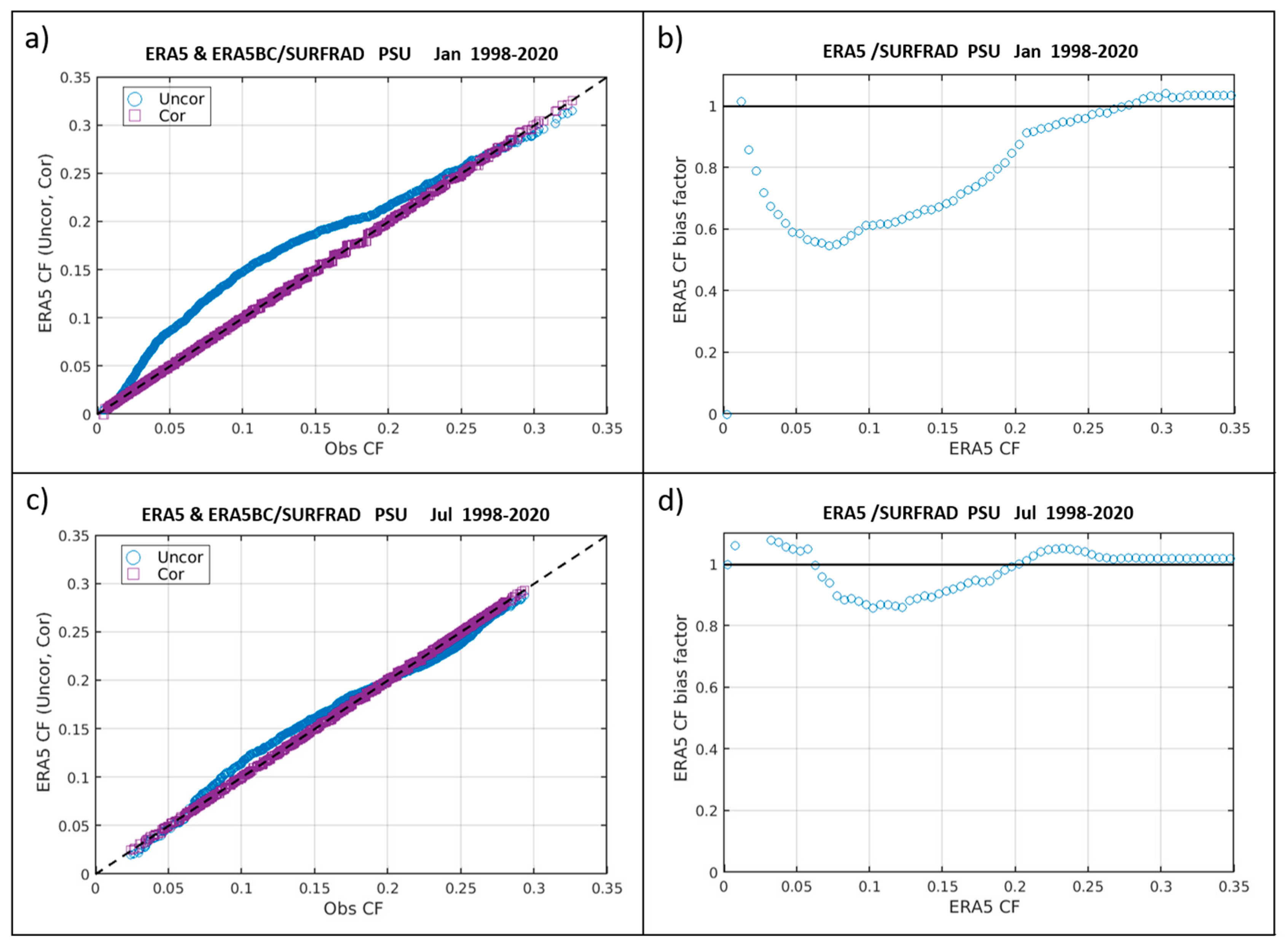
4.1. Quantile–Quantile Correction of Solar Power

The annual cycle of daily solar power CF for the SURFRAD PSU site and the corresponding ERA5 data are shown in Figure 3a, averaged over the time period 1998–2020. ERA5 data are included only if the corresponding PSU daily values are present. We note that even after averaging over 23 years of observations, the two time series still have considerable day-to-day variability. To obtain a better, smoothed estimate of the annual cycle, we fit both the PSU and ERA5 annual cycle time series in a least squares sense to an algebraic expression consisting of four pairs of harmonics using QR factorization:
C F t = a 1 + a 2   c o s ω t + a 3   s i n ω t + a 4 cos 2 ω t + a 5   s i n 2 ω t + a 6   c o s 3 ω t + a 7   s i n 3 ω t + a 8   c o s 4 ω t + a 9   s i n 4 ω t
where ω = 2 π / 365   d a y s . We find that 4 sets of harmonics, which allow for 4 maxima and 4 minima through the annual cycle, closely follow the 23-year average of the solar radiation data, while allowing for sub-seasonal anomalies to be fully represented.
The ERA5 and PSU capacity factor harmonic curves shown in Figure 3a agree well during the warm season months of June through September, but diverge in the cooler months from October through May, with the ERA5-derived values being up to 30% too large in December and January. The ERA5 clearly has a seasonally varying bias error, overestimating the true solar power in all but the summer months. Scatter plots of the ERA5-derived versus PSU daily solar CFs are shown in Figure 3c. The ERA5-derived CF values are in fairly close agreement for both small (overcast) and large (clear-sky) values, but are considerably greater than the observations for most mid-range CF values. Results in Figure 3a,c indicate that ERA5 solar CF errors are a function of season as well as CF magnitude. A seasonally dependent correction of the ERA5 CFs is therefore appropriate. We note that because the ERA5 and observations are in close agreement for completely overcast days when the CFs of both are near zero (Figure 3c), simply subtracting the day-of-year (DOY) biases from the ERA5 values is not a viable alternative because it would result in non-physical negative CF values for these overcast conditions.
Various methods have been proposed to correct the model, reanalysis, or satellite-based irradiances using in situ observations. Polo et al. [32] provide a thorough review of these methods, including linear regression [33,34], model output statistics (MOS) [35,36], cumulative distribution function (CDF) adjustments [37], and measure–correlate–predict (MCP) approaches [34]. In addition, Ruiz-Arias et al. [38] propose a method in which gridded estimates of solar radiation are corrected in the vicinity of ground observations based on the structure of the spatial covariance of the errors in both the gridded data set and ground observations. In the present analysis, the seasonally varying ERA5 errors are corrected using a standard quantile–quantile post-processing method (QM) that has been often used for climate and weather models [39,40,41,42,43,44,45], which is functionally equivalent to the CDF adjustment technique. Cannon et al. [46] discuss the application of QM to climate models’ projections of precipitation that have large trends and show that modified QM approaches (QDM and DQM) can be superior for correcting extreme values. However, for solar irradiances, the observed trends on continental scales are small and change signs on decadal time scales [47], while for hub-height winds the observational record is too short to accurately quantify long-term trends. Therefore, standard QM is used, and the ability of QM to accurately correct extreme solar and wind energy anomalies is demonstrated. Details of the QM procedure are provided in Appendix A.
The impact of the QM bias corrections on the CF annual cycle is seen in Figure 3b,d. The ERA5 Bias Corrected (ERA5BC) and PSU 4-harmonic curves are in excellent agreement and the DOY average values have similar ranges of values (Figure 3b). The ERA5BC has a smaller bias, MAE, and RMSE, a slope closer to unity, and an increase in correlation from 0.90 to 0.92. In addition, the standard deviations of the ERA5BC CFs are in much closer agreement with the observations (PSU = 0.084, ERA5 = 0.076, ERA5BC = 0.084).
Histograms of the ERA5, ERA5BC, and PSU CF values further demonstrate the improvement after QM correction (Figure 4). For the annual period (left panels), the uncorrected ERA5 is seen to have too few occurrences of small CF values, and too many moderately large CF values. The lack of small CF values is principally due to ERA5 errors occurring in the winter months (DJF, center panels), while the excess ERA5 moderately high values (CF ~ 0.2) occur in both winter and summer (JJA, right panels). For annual, winter, and summer evaluation periods, the QM correction brings the ERA5BC histograms into excellent agreement with the observations (Figure 4d–f).
Mean annual cycle solar CF plots were generated for all 13 SURFRAD/SOLRAD sites together with those for the aggregate of the 28 ARM-SGP sites (Appendix A, Figure A3). The ERA5 error characteristics for each of these sites are very similar to those found at the SURFRAD PSU site, namely that the ERA5 underestimates solar CFs during the autumn, winter, and spring, with a near zero or significantly reduced bias during summer. Annual quantile–quantile plots (Appendix A, Figure A4) also show a high degree of similarity across all sites, with a tendency for slightly larger deviations from the 1-1 slope for sites in the southwestern U.S. We note that the similarity of the ERA5 errors across the CONUS would make it relatively easy to spatially interpolate bias corrections from these sites to the entire ERA5 grid.
Summary statistics (NMB, RMSE, correlation coefficient, and the ratio of standard deviations) for the ERA5 and ERA5BC solar evaluation over all months of the year (Appendix A, Figure A5) show a consistent improvement resulting from the QM corrections. Although annual average solar CF NMB values range from about 5–15%, because the ERA5 biases vary with season, winter NMB values are found to be approximately twice as large, averaging +23% for all of the SURFRAD/SOLRAD sites, with the largest bias of +47% for Seattle (SEA). Also, the highest correlation coefficient (0.94) is found for the ARM-SGP aggregate. The aggregation process reduces the impacts of spatial variability and indicates that for even small-sized grid balancing areas, the system-wide solar generation for a dispersed set of generators would be very accurately estimated by the corrected ERA5.

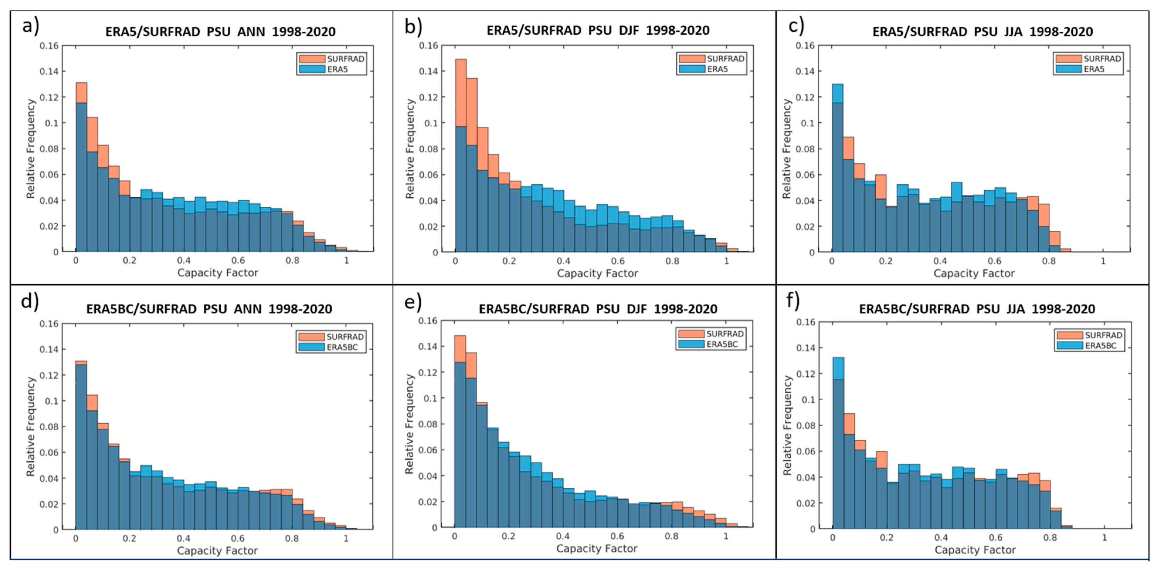
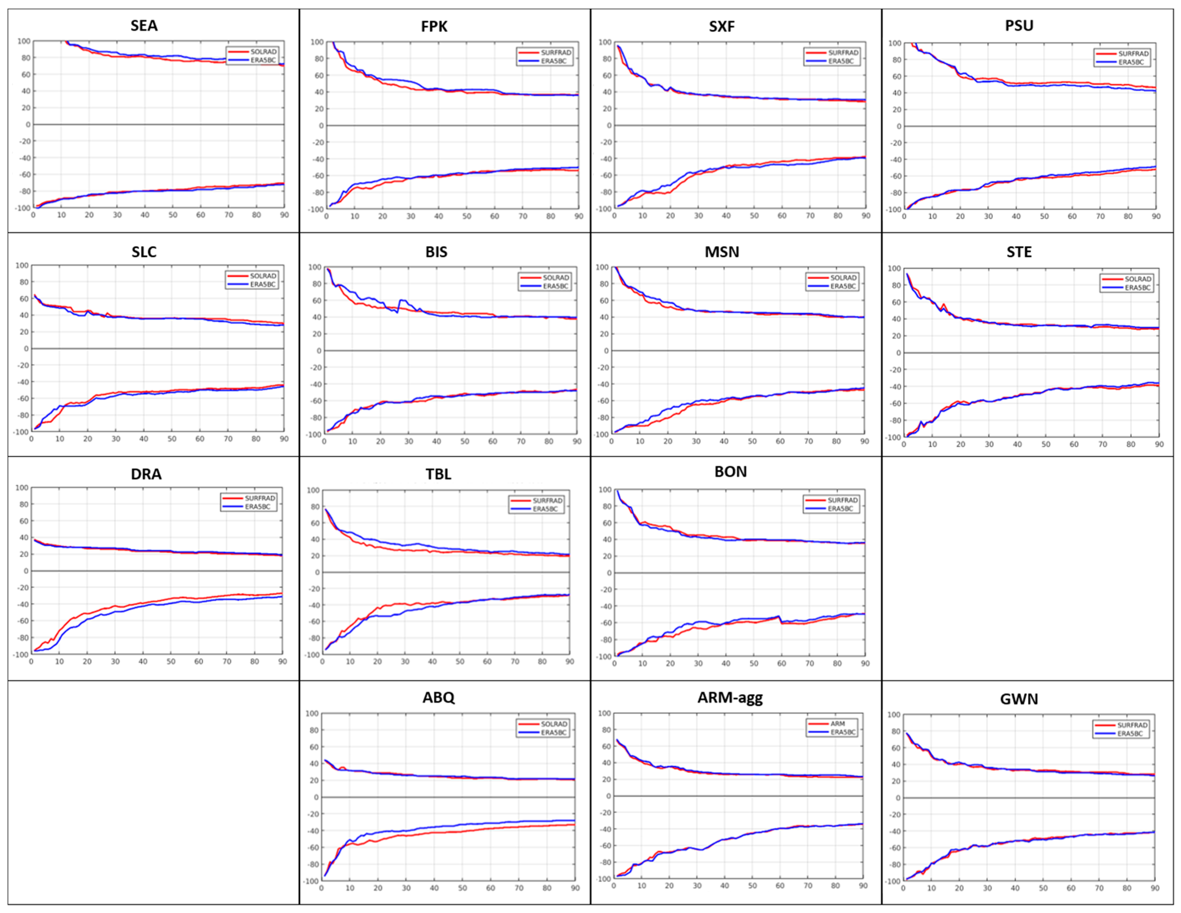
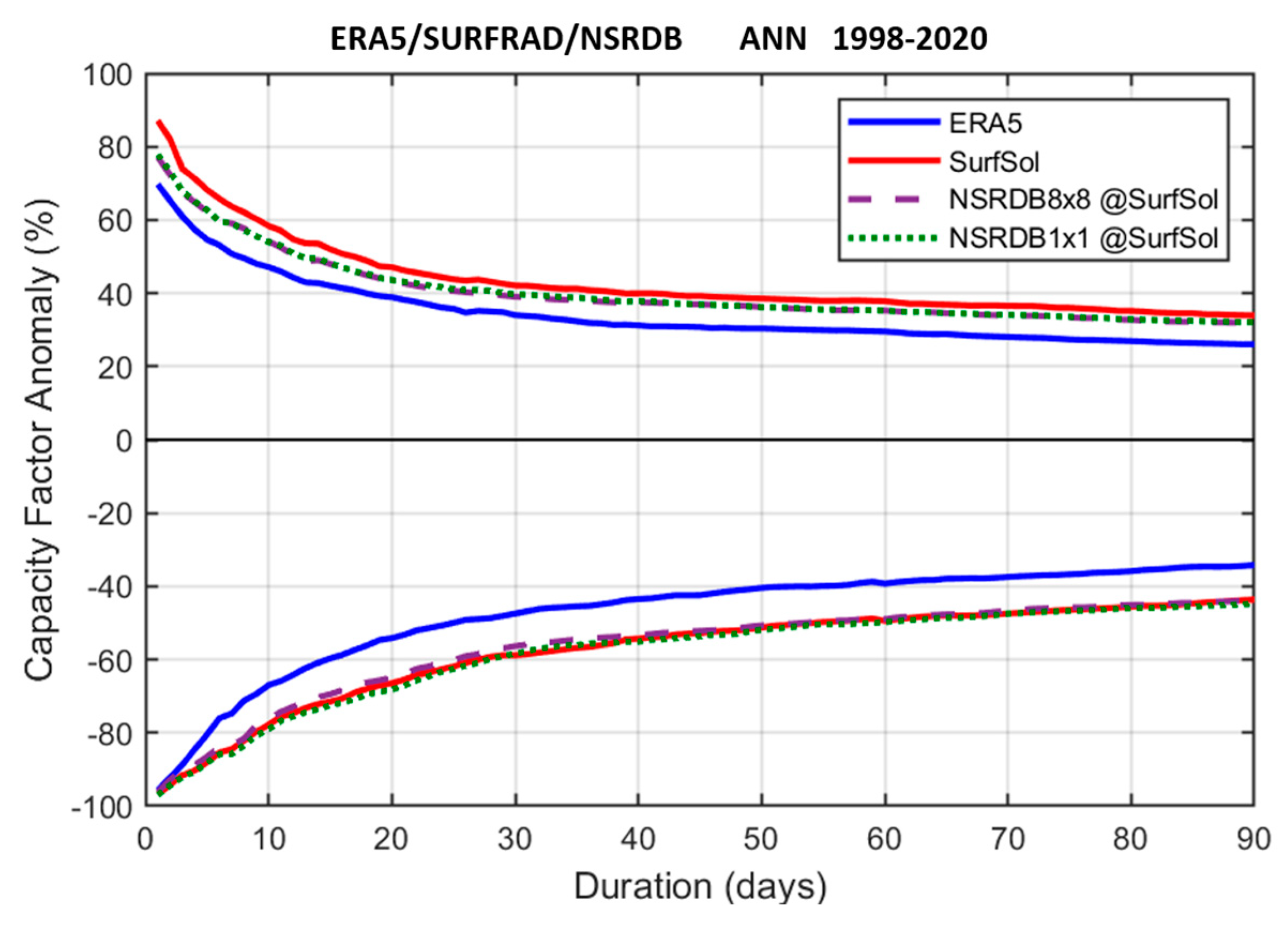
4.2. Intensity–Duration Curves

Of particular importance for grid integration studies is knowledge of how accurately the ERA5 replicates the most extreme low and high wind and solar energy events. Periods with the lowest wind and solar generation will determine how transmission, storage, and overbuilding of capacity will need to be configured in order to ensure that energy generation will be able to match load. Periods with the highest wind and solar generation provide valuable information on grid congestion, as well as on potential curtailment of generation if no methods are found to make use of the excess generation. We note that the results of capacity expansion model studies (e.g., [48,49,50]) that require generation to always meet load will depend crucially on these most extreme events.
A useful way to evaluate the ERA5-derived CF extreme values is through intensity–duration (I-D) curves, as shown in Figure 5 for the SURFRAD PSU site. Although there are many different approaches in the hydrology literature to calculate I-D curves, the approach we use focuses on the question of whether the corrections applied to the ERA5-derived CFs improve the observed extreme events that will be most impactful for grid operations. I-D curves are generated at each observation site by first calculating the time series of CF anomalies for each day of the 23-year period of SURFRAD observations. The observed anomalies are the differences between daily observed CF values and the 23-year mean observed CF value, while the ERA5-derived anomalies are the differences between the daily ERA5 CF values and the corresponding ERA5 mean CF over the same period. Next, the observed anomaly values are normalized by the corresponding observed mean CF value and the ERA5-derived CF anomalies are normalized by their corresponding ERA5-derived mean CF value. Both are then expressed as a percent. Mathematically, the anomalies are given by C F o b s a n o m t i = 100 × ( C F o b s t i C F o b s ¯   ) / C F o b s ¯ and C F e r a a n o m t i = 100 × ( C F e r a t i C F e r a ¯   ) / C F e r a ¯ , where t i is a serial day counter over the 23 years of observations, C F o b s ¯ is the mean observed capacity factor over that time period, and C F e r a ¯ is the ERA5 mean capacity factor over the same time period. Running means with windows varying from 1 to 90 days duration are then applied to the time series of the daily normalized CF anomalies. Next, the most negative occurrence is found within each of these smoothed time series, with the center point in the window taken as the time stamp for this worst “drought” event. Because of occasional missing observation data, at least 85% of the observed data are required to be present in any given window in order for that minimum value to be selected. It is not required that the worst-case anomalies be independent for each duration value, and, in fact, they most often contain overlapping data. Anomalies defined in this way do, however, characterize what the most extreme observed and ERA5-derived power anomalies are for any duration from daily to seasonal. The same procedure is then applied finding the maximum values in the smoothed anomaly time series, corresponding to the highest generation scenario. This method of calculating extremes focuses on the worst event of any duration in the time period analyzed, under the expectation that the energy system and grid would need to be designed to handle such an extreme scenario.
The I-D curves for the SURFRAD PSU site (Figure 5) have anomalies near −100% for a duration of one day, for both the observations and ERA5, simply indicating that both have completely overcast days when very little solar power would be produced. These anomaly values become more positive with duration as sunny or partially cloudy days enter the time-averaging window. At 90 days duration, the magnitude of the anomalies is largely determined by the amplitude of the seasonal solar cycle. The I-D curves also show that the ERA5-derived values underestimate the intensity of the negative solar anomalies for almost all durations longer than 5 days, and underestimate the positive anomalies for all durations. The magnitudes of these errors can exceed 25% of the observed anomalies.
I-D curves for each of the SURFRAD, SOLRAD, and spatially aggregated ARM-SGP solar sites are shown in Figure 6. The panels are arranged based on geographic location, with the more northern sites in the upper panels and the western sites in the left panels. In general, the agreement is good for events of one to several day’s duration when overcast conditions reduce solar power to near zero. However, as for the PSU site, for durations of about a week or longer, the ERA5 consistently underestimates the magnitudes of the normalized anomalies, both positive and negative, often by as much as 20–30%. QM correction (Figure 7) eliminates the consistent underestimation of the solar CF positive and negative extreme normalized anomalies with the two sets of curves now in close agreement at each site. Although the QM corrections were applied to daily data, they provide accurate estimates of extreme events for durations from one day to several months. The full characterization of a drought event requires having an accurate mean annual cycle and accurate extreme anomalies. The QM corrections provide both.

4.3. NSRDB and SURFRAD

To address the issue of the potential for erroneous inflation of the ERA5 CF variability resulting from the QM correction technique, we make use of an alternate data set, the National Solar Radiation Database (NSRDB, [51]). The NSRDB is similar to a reanalysis data set in that it combines both observations and a model to derive an estimate of atmospheric variables. However, the NSRDB differs from the ERA5 in that it utilizes satellite cloud observations together with a radiative transfer model, from which it estimates surface values of the GHI, DNI, and DHI irradiances on a 4 km horizontal grid. In contrast, observed cloud fields do not directly impact radiation estimates in the ERA5, and are only used to provide wind velocity estimates through cloud feature tracking. Using the NSRDB irradiance estimates together with ERA5 values of surface temperature, wind speed, and albedo, we calculate solar CF values and normalized anomalies, in the same manner as before, for each NSRDB grid point closest to the 13 SURFRAD/SOLRAD sites shown previously in Figure 1. Next, using an 8 × 8 grid of NSRDB values centered around each SURFRAD/SOLRAD location, the area mean GHI, DNI, and DHI values are calculated. With the NSRDB 4 km resolution, these 64 points correspond to approximately one ERA5 grid cell at its 31 km native resolution. The area mean NSRDB irradiances are used to calculate solar CFs and normalized anomalies for each of the 13 SURFRAD/SOLRAD sites, which are then averaged to form network mean values.
Figure 8 shows the resulting I-D curves for the four separate estimates (SURFRAD/SOLRAD, ERA5, NSRDB single closest grid cell, NSRDB 8 × 8 grid cell area average) of the largest anomalies. Both the single value and area-averaged NSRDB estimates are found to be in close agreement with the SURFRAD/SOLRAD values, and all three have greater anomaly amplitudes than the uncorrected ERA5. Importantly, the differences between the NSRDB 8 × 8 area average and single closest grid cell values are negligible, with the 8 × 8 averages having only slightly smaller amplitudes. This indicates that any erroneous over-inflation of the ERA5-derived CF values resulting from the QM correction is small enough to not materially impact a solar anomaly (drought) analysis. We note that the potential for QM correction-induced over-inflation is reduced by using daily averaged CF values. It is possible, if not likely, that applying similar correction techniques to hourly CF values would result in a significant over-inflation of reanalysis variances. However, since the daily average-based seasonally varying correction factors are multiplicative, one approach to correct hourly ERA5-derived solar CF values (if hourly values were desired) is simply to apply the correction determined with daily averaged values to each hour of the day. In essence, this assumes that the percentage biases in the ERA5 do not strongly depend on the hour of the day. Comparisons of QM plots and histograms using hourly data for the SURFRAD PSU site are shown in Appendix A, Figure A6 and Figure A7, which demonstrate that significant improvements to the hourly data are obtained using this method. In addition, at every SURFRAD and SOLRAD site, the correlation coefficient, bias, MAE, and RMSE all improve after applying the daily average-derived corrections to hourly values, demonstrating that this is a viable method for correcting hourly ERA5 values.
Returning to the mean errors between the observed and ERA5-derived anomalies averaged over the 13 SURFRAD/SOLRAD sites in Figure 8, the magnitude of the anomaly errors at any given duration can be referenced either to the amplitude of the observed anomaly or to the observed power produced, which is 100% plus the negative anomaly value (for negative anomalies). At 10 days duration, the negative CF anomaly error is (ERA5 CF anomaly—Observed CF anomaly) = −(67% − 79%) = 13%, which for the first option, is 16.5% of the 79% observed anomaly. However, for the second option, the observed power produced is (100% + Observed CF anomaly) = (100% − 79%) = 21%, and 13% is 62% of the 21% observed power produced. This second interpretation option would be appropriate if one were to ask how much overbuilding of generation capacity would be needed to compensate for the drought anomaly and shows the large impact that the ERA5 errors can have when determining how to mitigate droughts.
Finally, it is noted that although the I-D evaluation focused on the most extreme event at each duration in the observation time period, similar analyses have been conducted for less extreme values. Whereas the single worst event for the 23 years in the PSU observation record has, by definition, a return period of 23 years, in Appendix A, Figure A8, I-D curves are shown for the average of the 10 most extreme anomaly events, which are then the averages of all of the anomalies with return periods longer than 2.3 years. The overestimation of the anomaly events by the ERA5-derived CF values is still present, while the QM-corrected values (ERA5BC) are in very close agreement. A general finding is that the agreement between the observations and QM-corrected values is better for shorter return periods than for the single most extreme anomaly event.

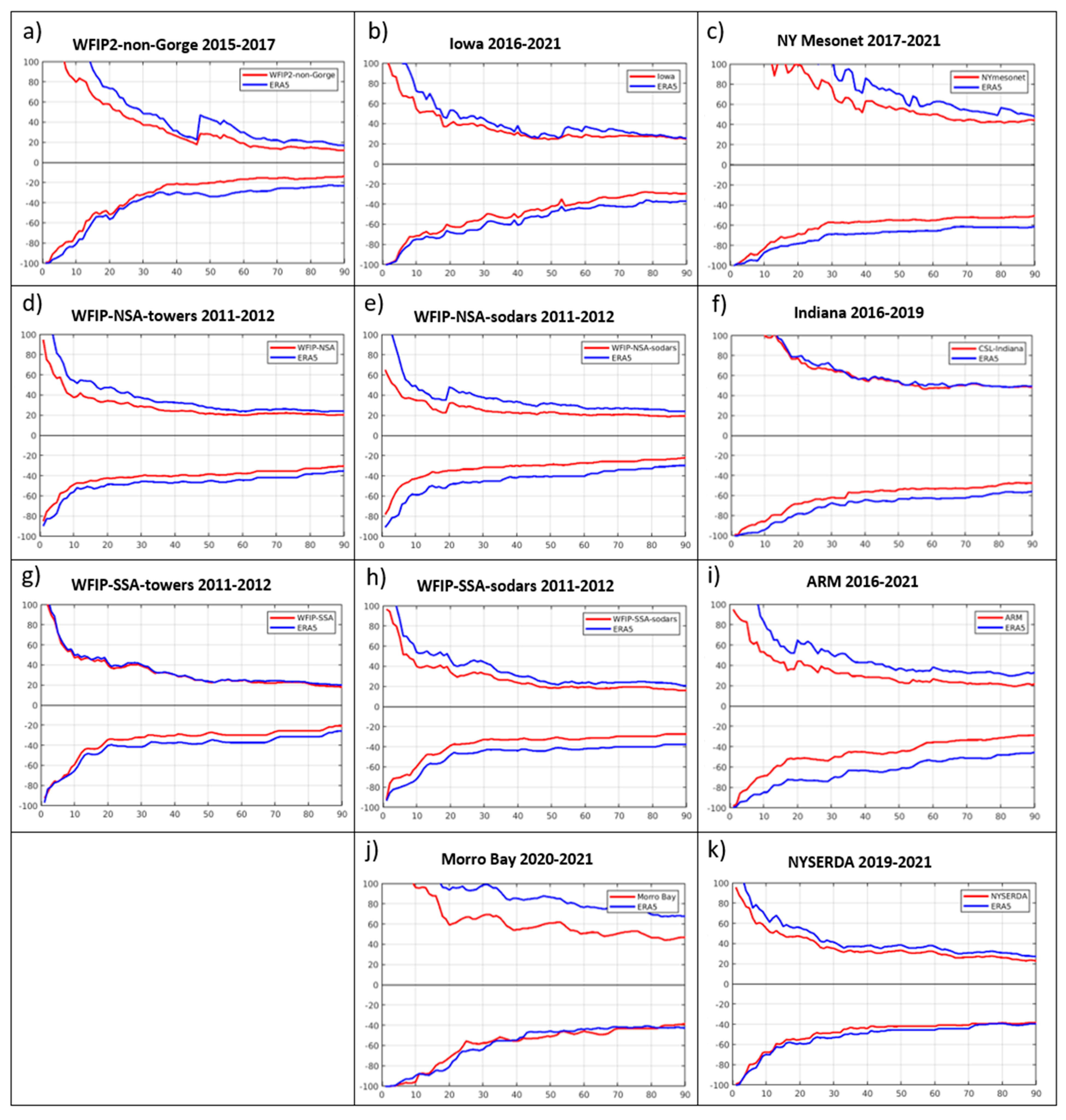
5. Evaluation of ERA5-Derived Wind Capacity Factor Systematic Errors
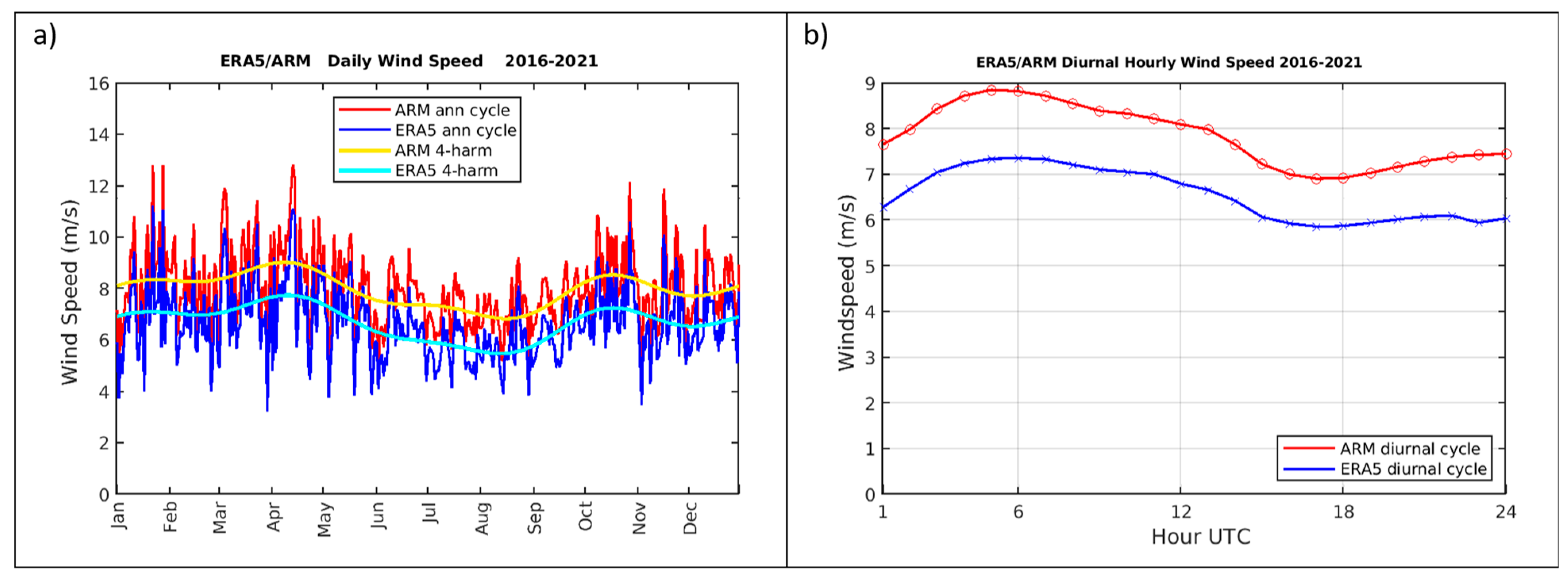
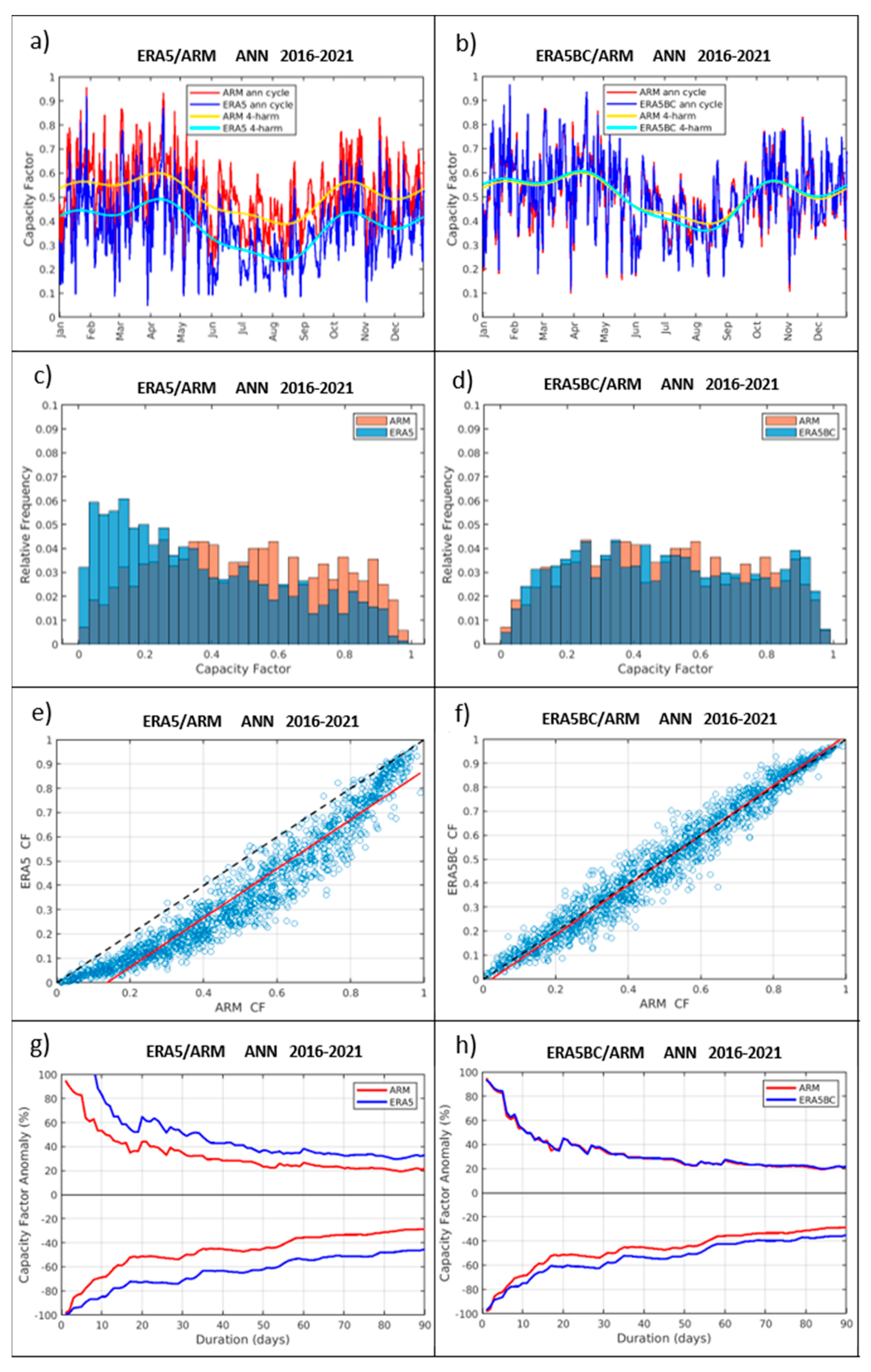
Although a varying density is included in our wind power calculations, we assume that systematic errors in wind power values result only from errors in wind speed, not density. This is because temporal variations in wind speed frequently produce changes in power from zero to near 100% of maximum power capacity, while density temporal variations typically range between +/− 10%, possibly reaching +/− 20% seasonally. In addition, the weather models used for reanalyses are carefully tuned to produce accurate estimates of near-surface temperature (from which, together with pressure, density is derived). Therefore, we assume that systematic ERA5 errors in density will have a small impact on wind power errors. Because the systematic wind power errors are then dependent on a single model variable (wind speed), we choose to evaluate and correct wind speed in order to obtain wind power that is unbiased, has the correct variability, and can be used with any wind turbine power curve.

5.1. ARM-SGP Lidars

As the same analysis procedure is applied to each of the wind data sets analyzed, we provide a detailed description of this process using one of these (the ARM-SGP lidars), and then also provide summary figures comparing all of the data sets. The DOE ARM program has operated a small network of vertical profiling lidars at the SGP facility since 2016, consisting of 4 sites (E32, E37, E39, and E41) that form a square approximately 60 km on a side, centered on the SGP central facility where a 5th lidar is maintained [52]. Although none of the lidar data have been assimilated into the ERA5 reanalysis, radiosondes are launched 4 times per day from the ARM-SGP central facility [53], which were assimilated into the ERA5 (Hersbach, personal communication), and, therefore, the collocated lidar wind profiles from this site are excluded from the analysis.
The first two lidar measurement heights are 90 and 116 m, which were linearly interpolated to 100 m. Six 10 min averages of scalar wind speed are nominally available each hour, and a minimum of 3 values were required to form a valid hourly average, centered on the hour. Wind CFs were then computed using the hourly averaged wind speeds and using the wind turbine power curve classification consistent with the annual average 100 m wind speed for each site. Daily averages of wind speed and power were then computed, requiring at least 4 daytime and 4 nighttime hours to be present in order to reduce potential biases associated with any diurnal variation of wind power. In addition, daily averaged values from a minimum of 3 out of the 4 sites were required to be present to form a daily aggregate value. ERA5 hourly wind speed values were time-matched with the hourly observations, and the hours in which the observations were missing were excluded. ERA5 aggregate values of the daily mean wind speed and power were then computed as was carried out for the lidar observations. For evaluation purposes, the same power curve at each site was used for both the observations and ERA5, and the turbine high-speed cutout was not applied to avoid the circumstance of one of either the ERA5 or observations being just above the threshold and the other below, resulting in power values of 1 and 0, even though the difference between the two wind speeds is small.
The annual cycle of daily wind speed is shown in Figure 9a. Six-year means for each day of the year for the period of 2016–2021 were calculated for the observations and the ERA5, along with their corresponding four-harmonic fits. An ERA5 wind speed low bias of ~1.3 ms−1 is apparent, which is nearly constant across all seasons of the year. The diurnal variation of wind speed (Figure 9b) shows that differences between the ERA5 and observations are nearly constant across the diurnal cycle. This indicates that using corrections based on daily aggregate values would be appropriate, and also suggests that ERA5 wind speed low biases are not due to stability effects, but more likely due to surface roughness estimates or some other parameter that is diurnally independent.
Scatter plots of the ARM-SGP lidar 4-site aggregate of daily mean wind speed and CF values are shown in Figure 10i. The ERA5 wind speeds are consistently low for all values of wind speed. An orthogonal least squares linear fit has a slope of 0.94, indicating that the ERA5 also has slightly too little variability, and a correlation of 0.979, demonstrating that other than the systematic offset, the ERA5 has very high skill at replicating the observed daily wind speeds at these sites. We note that for the ARM-SGP aggregate, the −1.29 ms−1 ERA5 bias is equivalent to a normalized mean bias (NMB) of −16%, but that after applying the appropriate power curve, this translates to a wind CF NMB of −27%. Using the least squares fits to the daily aggregate wind speeds, corrections are then applied to the hourly wind speeds, and wind power is then calculated from the corrected hourly values. Staffel and Pfenninger [54] also applied linear regression to bias correct the MERRA reanalysis, but in their analysis, they derived wind speed corrections needed to match the known regional wind power generation, rather than observed wind speeds.
The annual cycle of wind CF for the ARM-SGP aggregate is shown in Figure 11, both before (Figure 11a) and after the linear regression correction (Figure 11b). Without correction, the ERA5-derived wind CFs are biased low by 0.14, which is the opposite sign of the ERA5 high-bias found for solar CF for most seasons. The correction results in near-perfect agreement through the complete annual cycle. Histograms of the daily wind CF values (Figure 11c) indicate that the ERA5 produces too many low CF days and not enough mid-to-high CF days compared to the ARM observations. After applying the linear regression correction, the histograms of ERA5BC and the observations are in very close agreement (Figure 11d). Scatter plots of CF values show the uncorrected ERA5-derived values are too small except for extremely small and large values (Figure 11e) and are in close agreement after applying the linear regression correction (Figure 11f). I-D curves show that the ERA5 overestimates the magnitudes of both the most negative and positive anomalies for almost all durations (Figure 11g), with the negative anomalies being as much as 40% larger than the observed values on monthly or longer timescales. In terms of power produced (100% minus the anomaly value), at 10 days duration, the ERA5-derived wind power produced is less than half the observed power, highlighting the significant impact that the ERA5 errors can have during wind drought events. The linear regression correction greatly reduces these errors (Figure 11h).

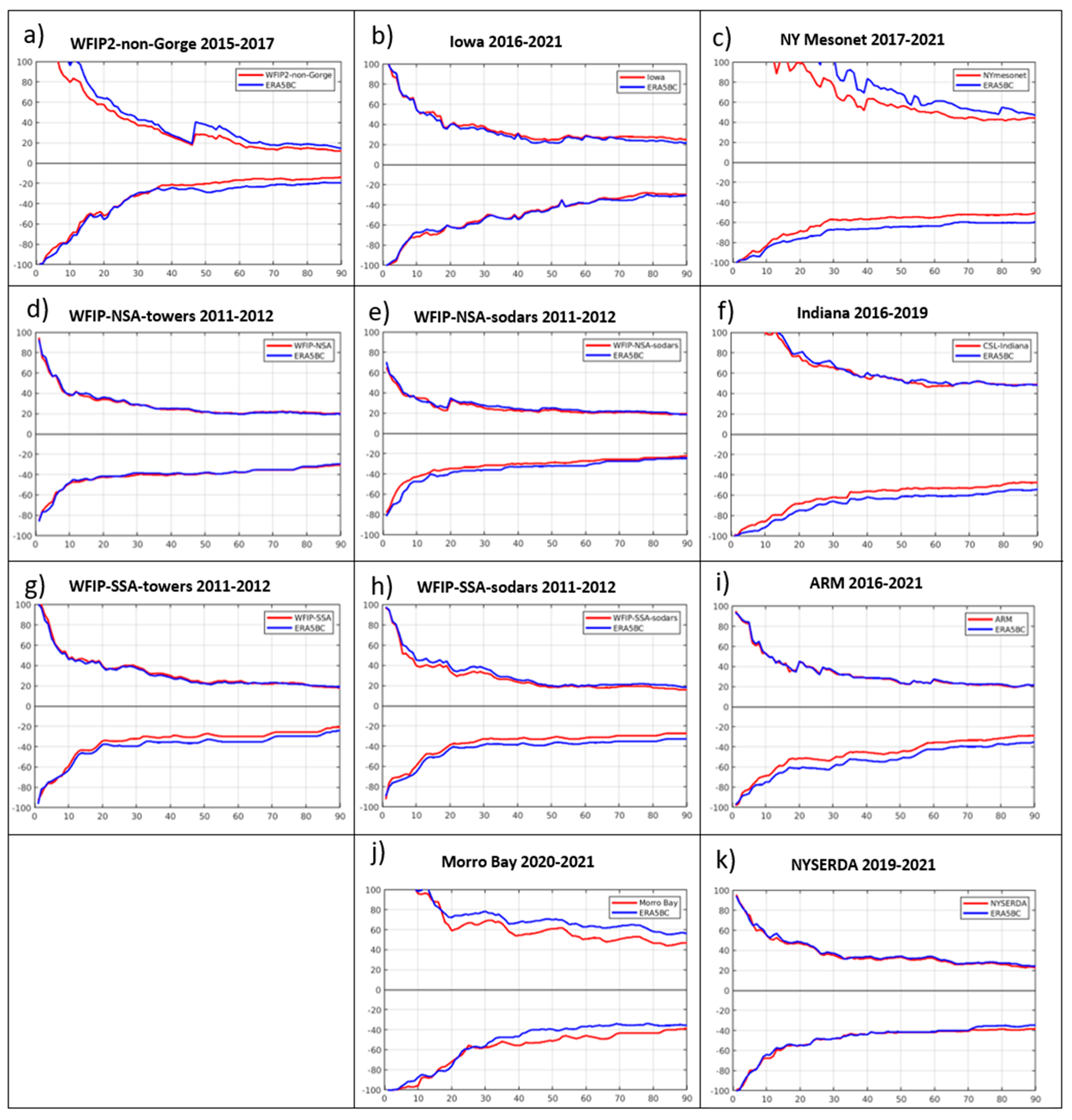
5.2. Corrections to the Remaining Wind Data Sets

To assess whether a similar correction could be applied to the ERA5 across the entire analysis domain, we repeat the same procedure using each of the wind data sets listed in Section 2.3. Details of the processing for each data set are provided in Appendix A.
Scatter plots of the daily average wind speed for each of the wind data sets are shown in Figure 10. For those data sets that have multiple observation sites, the spatial aggregate of the daily mean wind speeds is shown. At all land-based sites from the Pacific coast to Iowa, the scatter plots consistently have slopes less than unity, negative intercepts, and negative biases, with the 6-network (WFIP1 NSA towers, WFIP1 NSA sodars, WFIP1 SSA towers, WFIP1 SSA sodars, WFIP2 sodars and lidars, and ARM SGP lidars) average wind speed NMB being −12%, and the corresponding wind CF NMB = −20%. The negative biases occur regardless of whether the observations come from tall towers, sodars, or lidars. In contrast, further east the NYmesonet aggregate and the Indiana site both have slopes greater than unity, with small wind speed normalized mean biases of −1.8% and +3.9%, respectively. Scatter plots of daily average 100 m wind speed for the over-ocean wind data sets are shown in the bottom row of Figure 10. The aggregate of the two NYSERDA lidar buoys on the east coast [55], and the Morro Bay west coast lidar data sets both show similar ERA5 error characteristics, which also closely match those found over the central and western CONUS, with slopes less than unity and negative biases. Summary statistics (NMB, RMSE, correlation coefficient, and the ratio of standard deviations) for the ERA5 and ERA5BC wind evaluation (Appendix A, Figure A10) show a consistent improvement resulting from the linear regression corrections.
Intensity–duration diagrams for each of the wind data sets are shown in Figure 12 for the ERA5 and Figure 13 for the ERA5BC. The ERA5-derived values (Figure 12) display varying degrees of agreement with the observed values. As was shown for the ARM lidar data set, applying a linear wind speed correction specific to each of the individual data sets yields closer agreement between the ERA5BC-derived and observation-derived extreme anomalies, as depicted in the I-D curves.
A map of the mean ERA5 wind speed biases for each of the wind data sets is shown in Figure 14, individually for each observation site, except for the WFIP1 NSA and SSA tall tower sites, which are only shown in aggregate due to the large number of towers and because of data gaps in many of the individual tower data records. An ERA5 low wind speed bias is found to exist generally across the central and western U.S., similar to that shown previously for the ARM-SGP sites. The three offshore sites also show a negative wind speed bias. In contrast, although the number of observation sites is limited, in the northeastern U.S., the biases have a nearly equal distribution of positive and negative values.
An important consideration is the potential impact of wind farms themselves on the wind speed observations used to evaluate the ERA5. Wakes from wind farms can be substantial and can propagate for tens of kilometers downstream before they eventually dissipate [56]. Other than not including data from one WFIP1 sodar and one of the Iowa Atmospheric Observatory tall towers that were each collocated with wind turbines, the possible effects of wind plants are not accounted for. With the large numbers of wind farms now operating across the central U.S., it is likely that many of the observations used in our analysis are affected by them to some degree. For example, Bodini et al. [56] determined that several of the ARM-SGP lidars are impacted by nearby wind plants, decreasing the observed 100 m wind speeds by 4–6% during stable stratification. Given the number of wind farms and their growth over time, it would be a near-impossible task to correct their impacts on the observational data sets used. However, as can be seen in Figure 14, the ERA5 has a consistently low wind speed bias compared to observations across the central U.S. Wind plant wakes would decrease the observed wind speeds locally (limited in both the horizontal and vertical directions), while it seems unlikely that they would influence the ERA5 windspeeds that are driven by large scale pressure gradients. Therefore, the true ERA5 bias in the absence of wind plant wakes would only be worse, an even larger underestimate. Correcting the ERA5 based on the available observations is therefore clearly better than not correcting it. However, it is possible that the resulting higher ERA5BC wind speeds and wind CFs will still be lower than for the true non-waked flow.
Unlike for solar, where the high spatial resolution NSRDB data set could be used to evaluate possible excess inflation of the ERA5 grid cell values based on point measurement corrections, no such high-resolution data set exists for turbine-height winds within the analysis domain. One test that can be carried out, however, is to evaluate the effects of both temporal and spatial averaging on the least squares regression-based correction. For this purpose, wind speed slopes were determined for the seven networks of wind observations (ARM-SGP lidars, WFIP1 NSA and SSA tall towers, the WFIP1 NSA and SSA sodars, the WFIP2 sodars and lidars, and the NYmesonet lidars), for four levels of averaging: hourly non-aggregate, hourly aggregate, daily non-aggregate, and daily aggregate. The averages of these slopes are 0.83, 0.93, 0.91, and 0.96, respectively. The smallest mean slope corresponds to the least amount of temporal or spatial averaging, and the largest slope for the greatest amount of averaging. This is a result of the phenomena of regression dilution, which is the biasing of the linear regression slope toward zero caused by errors in the independent variable. In the present analysis, the errors of the independent variable are in part a result of using point measurements, which may sub-sample small-scale spatial variability, to compare to an ERA5 value. The larger slope for the aggregate of the daily averaged speeds compared to the non-aggregate daily averaged speeds indicates that correcting the ERA5 with daily averaged speeds from individual non-aggregated stations would over-inflate the ERA5 variability by about 5%. Correcting the ERA5 with hourly non-aggregate linear regression would be significantly worse, with the ERA5 variability being over-inflated by 13% compared to the daily spatial aggregate. To reduce the impact of regression dilution we use only orthogonal linear regressions of spatial aggregates of daily averaged wind speeds to correct the ERA5. We also note that although regression dilution can change the slope and intercept, the overall bias is not affected.
Having derived site-based corrections to the ERA5-derived solar CFs and wind speeds, an important question is how one could translate those site-dependent corrections onto the entire ERA5 grid within the analysis domain. For solar CFs, the spatial uniformity of the binned bias corrections shown in Figure A4 indicates that this would be a trivial exercise, and almost any type of spatial interpolation procedure would produce reasonable results. For wind speed, there is greater spatial heterogeneity, but perhaps more importantly, the available observations are geographically clustered. Clearly, however, in the high-wind resource areas in the central U.S. and for offshore locations, correcting the ERA5 underestimation of hub-height wind speeds is necessary.

6. Summary and Discussion

Errors in ERA5-based estimates of daily averaged wind and solar energy generation have been quantified using observed and ERA5 meteorological variables. For solar irradiances, although the ERA5 errors for global horizontal irradiance are small, there are large compensating errors in its direct beam (NMB = +25%) and diffuse (NMB = −18%) components. These errors lead to corresponding systematic errors in derived solar capacity factors for solar panels that are tilted off the horizontal plane towards the sun. For solar panels that have a fixed tilt that optimizes the annual energy production (assumed in this study), the ERA5-derived CFs have a seasonally varying positive bias that is largest in winter (NMB = +23%) and smallest in summer. These errors are found to have consistent characteristics across the CONUS region.
Systematic errors for 100 m wind speed are also found in the ERA5. Negative bias errors in the ERA5 wind speeds and CFs are generally consistent across the central and western U.S., and offshore, usually with little seasonal or diurnal variation, while the northeastern U.S. has an overall small net bias. Wind speed NMB values average −12% across the central and western U.S., with a corresponding wind CF NMB average of −20%. Overall, solar CFs are biased high in the ERA5, and wind CFs are biased low.
Errors for the shortest duration, most extreme solar negative anomaly events (i.e., solar energy droughts) are found to be small when completely overcast conditions occur in both ERA5 and observations. Longer duration events on weekly to monthly timescales, which include partially cloudy days or a mix of cloudy and clear-sky days, have significant ERA5 errors. At 10 days duration, the ERA5-derived solar power produced during the largest anomaly events is 62% greater than observed, when averaged over all of the SURFRAD and SOLRAD sites. For the ERA5-derived most extreme negative anomaly wind power events, at some sites at 10 days duration, the ERA5-derived wind power produced can be less than half of that observed. The ERA5 errors, if uncorrected, could therefore significantly impact any ERA5-based wind and solar drought analysis.
Four potential sources of the identified discrepancies between ERA5 and observations are:
(1)
Instrumentation errors: Although this possibility can never be completely ruled out, this seems unlikely, as only the highest quality observational data sets available have been used, and for wind, similar errors are found whether using sodars, lidars, or tall tower in situ observations.
(2)
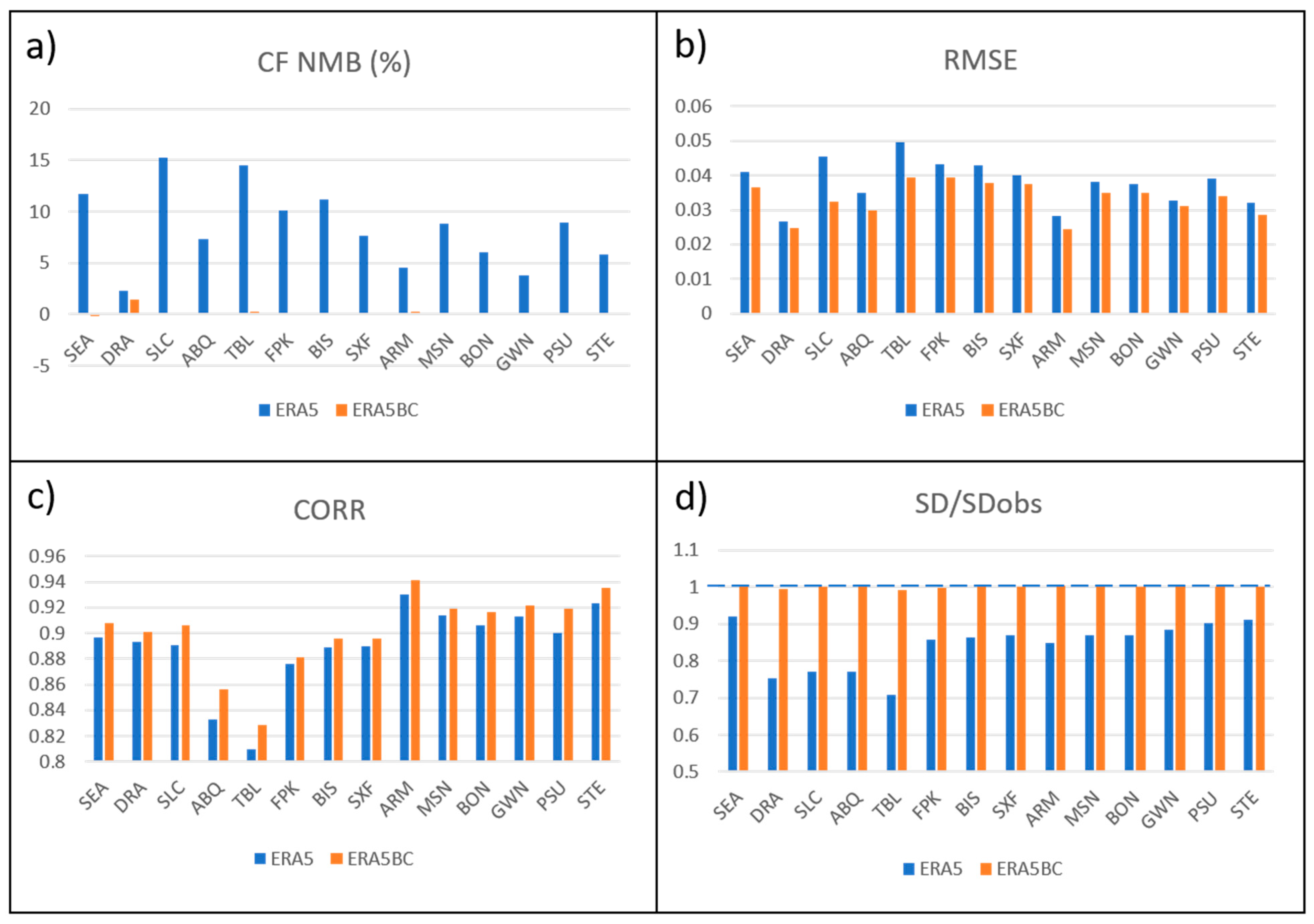
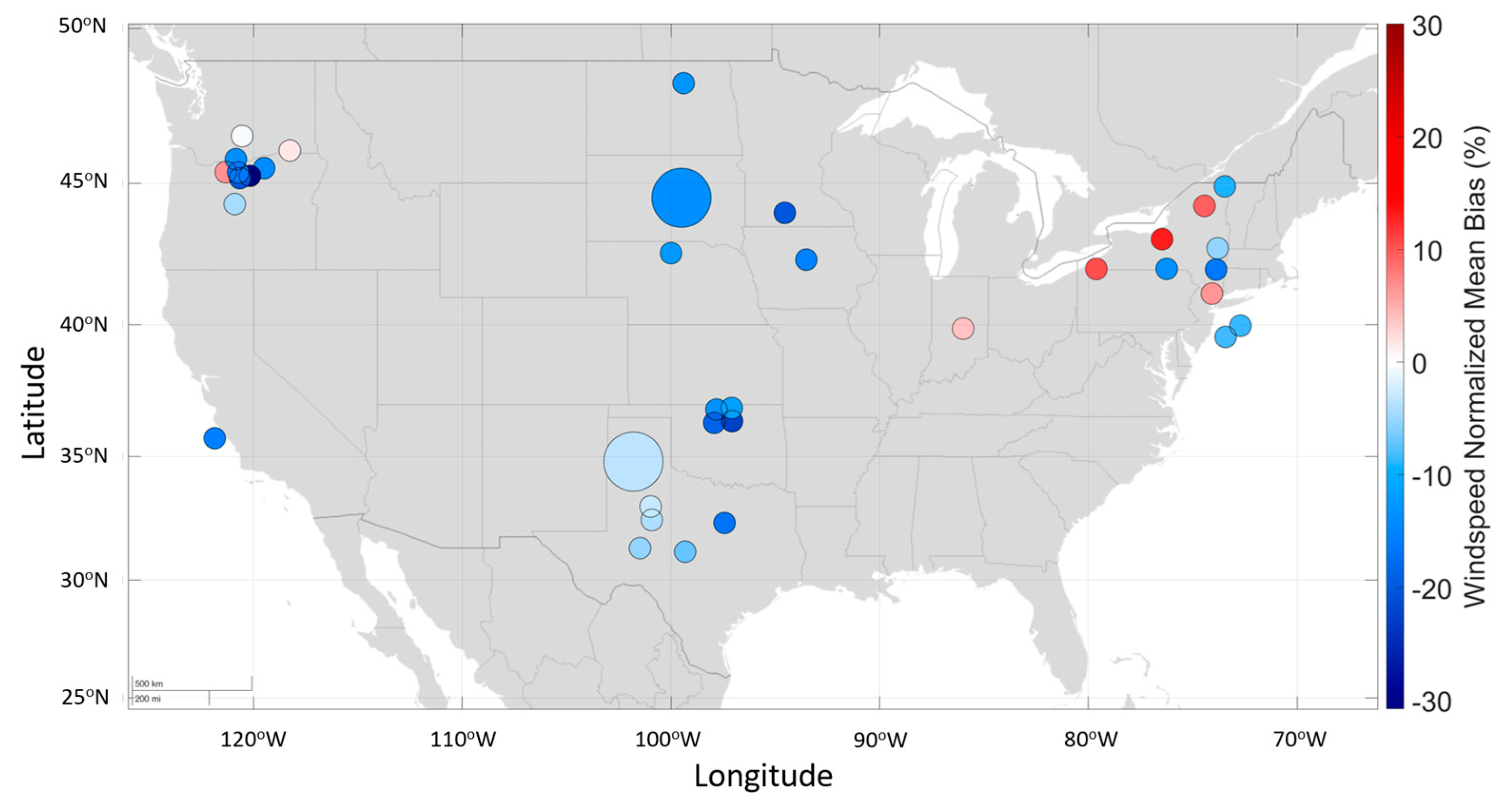
Non-representative siting within a grid associated with topography or land surface conditions: For solar, similar systematic errors are found for all sites, indicating that non-representative siting can be ruled out. For wind, in the central and western U.S., similar systematic errors are found whether in extremely flat (Iowa), flat but uniformly sloping (ARM-SGP) terrain, or more moderate rolling terrain (WFIP1, WFIP2). This indicates that it is unlikely that siting and terrain effects are a dominant source of the wind speed errors.
(3)
Turbine wake effects: Since the ERA5 does not account for turbine wake effects, the effect of wakes, if they are present, would be to bias the ERA5 winds higher than the observations, while instead they are found to have a low bias. Wind turbine wakes cannot therefore explain the ERA5 biases, and the true ERA5 biases, relative to unwaked flow, would be larger by some unknown amount if wind turbine wakes did not exist. The magnitude of the ERA5 wind speed negative bias, therefore, can be considered to be a lower bound and may be greater.
(4)
Model physical parameterization errors: Wind speed errors are not found to be a strong function of season or diurnal cycle, suggesting that stability impacts are not important, but also increase with wind speed, leaving surface roughness as a more likely source. Wind biases are larger for non-forested regions, and are smaller on average for the northeastern U.S., which is heavily treed, again suggesting a surface roughness parameterization error. For solar, ERA5 errors are smallest in summer months, while winter days that are partially cloudy are the most difficult, which may help identify aspects of cloud parameterizations that could be the source of these errors.
Two methods are presented for correcting the ERA5 errors, one for solar and one for wind. For solar, although one could choose to correct separately the DNI, DHI, and GHI, and then calculate solar power, we instead calculate solar power first and then correct it. This is both simpler and likely more accurate. The solar correction technique, based on quantile–quantile ordered pair plots, effectively reduces the solar CF biases across the annual cycle, brings the reanalysis and observed variability (standard deviations) into agreement, and produces intensity–duration curves of the largest amplitude anomalies that closely agree with the observations. Because of the geographic similarity of the ERA5 solar errors, corrections derived from the solar observation networks could be easily interpolated across the analysis domain. For wind power, wind speed corrections based on linear regression also reduce the wind CF biases across the annual cycle, bring the reanalysis and observed variability into close agreement, and produce intensity–duration curves of the largest amplitude anomalies that better agree with the observations.
The potential for erroneous inflation of ERA5 variances due to applying corrections from point measurements to grid cell values is investigated for solar using the high-resolution NSRDB tool. Results from this analysis indicate that when using daily averaged CFs, the quantile correction method does not create any significant over-inflation. In addition, the ARM-SGP aggregate results indicate that for even small-sized grid balancing areas, the system-wide solar generation for a dispersed set of generators would be very accurately estimated by the corrected ERA5, with correlation coefficients of daily CFs approaching 0.94. For wind, the potential for erroneous inflation of corrected ERA5 variances is investigated by examining the effects of both temporal and spatial averaging on the least squares regression-based correction. Comparing hourly non-aggregate, hourly aggregate, daily non-aggregate, and daily aggregate regressions indicates that, although the hourly non-aggregate data would result in over-inflation, that over-inflation is greatly reduced for the daily and spatially aggregated corrections used in this study.
In summary, the proposed correction methodologies would provide considerably more accurate estimates of the wind and solar resources, and the depiction of drought events, than those obtained using the uncorrected ERA5. Given that the ERA5 is widely considered to be one of the most accurate reanalysis data sets available, the findings demonstrate the importance of carefully evaluating and correcting systematic errors within model-based meteorological data sets, including climate models, which are used for resource assessment, grid integration, or drought analysis studies. Although the corrected ERA5-derived data better represent the observed statistics of wind and solar power, including the most extreme events, they still will suffer from the fundamental limitation of the ERA5’s coarse grid resolution. The effects of grid resolution will likely affect wind power estimates more than solar, as local topographic variations can have an acute impact on turbine-height winds, but less impact on clouds that are present through deep layers of the atmosphere. Ultimately, the best solution would be to have much higher resolution (~3 km) reanalyses, which could be directly compared against observations and then corrected. Finally, this analysis has benefitted greatly from the long-term observations provided by the geographically distributed NOAA SURFRAD, SOLRAD, and DOE ARM SGP solar networks. Building a continental-scale network of long-term, high-quality boundary layer wind observations would provide similar benefits for future renewable energy analyses.

Author Contributions

Conceptualization, J.M.W., G.P.C., A.C. and E.A.; Methodology, J.M.W., E.A., A.C. and G.P.C.; Software, E.A. and J.M.W.; Validation, J.M.W. and E.A.; Formal Analysis, J.M.W. and E.A.; Investigation, J.M.W. and E.A.; Resources, J.M.W. and E.A.; Data Curation, E.A. and J.M.W.; Writing—Original Draft Preparation, J.M.W.; Writing—Review and Editing, J.M.W., G.P.C., A.C. and E.A.; Visualization, E.A., J.M.W. and G.P.C.; Supervision, J.M.W.; Project Administration, J.M.W.; Funding Acquisition, J.M.W. All authors have read and agreed to the published version of the manuscript.

Funding

This work was funded by the NOAA Physical Sciences Laboratory and the NOAA Atmospheric Science for Renewable Energy program. This work was also supported in part by the NOAA cooperative agreement NA22OAR4320151.

Data Availability Statement

Data used in this study are available at the following URL/DOIs. NOAA SURFRAD, SOLRAD: https://gml.noaa.gov/grad/surfrad/ (accessed on 30 June 2022); https://gml.noaa.gov/grad/solrad/ (accessed on 30 June 2022); DOE SGP QCRAD solar irradiances: https://doi.org/10.5439/1227214 (accessed on 23 March 2022); WFIP1 sodars: https://a2e.energy.gov/data (accessed on 23 March 2022); WFIP2 sodars and lidars: https://a2e.energy.gov/data (accessed on 21 April 2022); DOE SGP lidars: https://doi.org/10.5439/1178582 (accessed on 22 March 2022); NYSERDA buoy lidars: https://oswbuoysny.resourcepanorama.dnv.com/ (accessed on 13 September 2023); DOE Morro Bay buoy lidar: https://a2e.energy.gov/ds/buoy/reanalysis.z06.c0 (accessed on 8 Sept 2023); NOAA CSL INFLUX Indiana lidar: https://csl.noaa.gov/projects/influx/ (accessed on 14 April 2022); Iowa Atmospheric Observatory towers: https://talltowers.agron.iastate.edu/ (accessed on 12 January 2022); ERA5: https://cds.climate.copernicus.eu/cdsapp#!/dataset/reanalysis-era5-single-levels (accessed on 1 February 2023). The following data are available through requests sent directly to the data owner: NYmesonet lidars, https://www.nysmesonet.org/weather/requestdata (accessed on 13 September 2022). The WFIP1 Northern Study Area tall tower data are proprietary to Next Era Energy and require a non-disclosure agreement from them. The WFIP1 Southern Study Area tall tower data are proprietary to ERCOT and require a non-disclosure agreement from them.

Acknowledgments

The authors thank Cathy Smith, Laura Riihamaki, Gene Takle, Dan Rajewski, Jerry Brotzge, Nathan Bain, Lindsay Sheridan, Alan Brewer, Dave Allured, Irina Djalalova and Tim Myers for their assistance in accessing various data sets used in the analysis, Hans Hersbach for providing information on data sets assimilated into the ERA5 reanalysis, and Laura Slivinski for reviewing the manuscript. Data were obtained from the Atmospheric Radiation Measurement (ARM) user facility, a U.S. Department of Energy (DOE) Office of Science user facility managed by the Biological and Environmental Research Program. The Iowa Atmospheric Observatory towers and associated instrumentation were funded by an NSF/EPSCoR grant to the state of Iowa (Grant #1101284) and a follow-on NSF/AGS grant #1701278. Original funding for the New York State (NYS) Mesonet (NYSM) buildup was provided by Federal Emergency Management Agency grant FEMA-4085-DR-NY. The continued operation and maintenance of the NYSM is supported by National Mesonet Program, University at Albany, Federal and private grants, and others.

Conflicts of Interest

The authors declare no conflicts of interest.

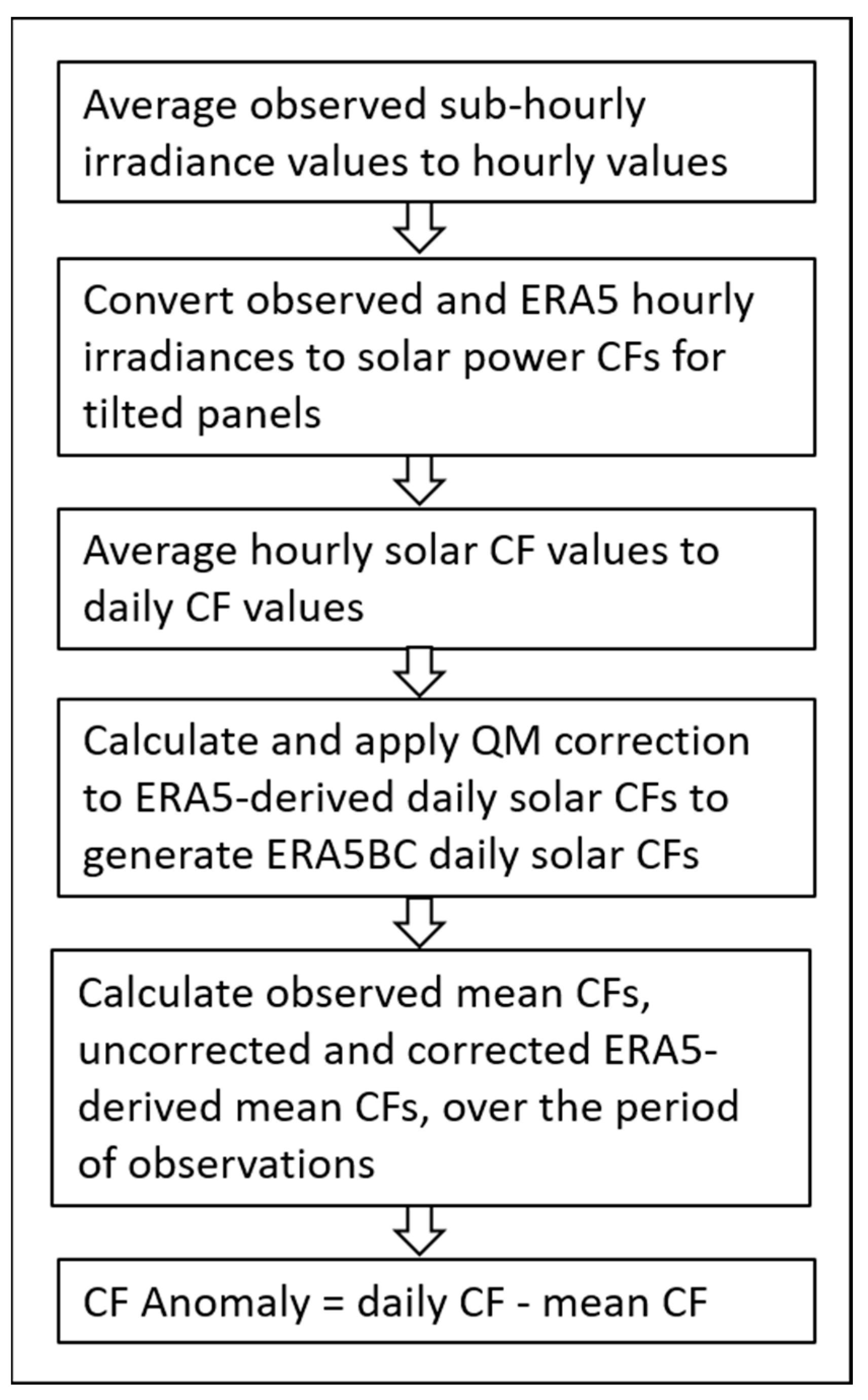
Appendix A. Processing Methods for Solar Power and Summary Statistics

Figure A1. Flow chart of processing steps to calculate daily observed, uncorrected ERA5-derived, and corrected ERA5-derived solar CFs and CF anomalies. In the last step, the anomalies are calculated independently for the observations, ERA5-derived, and corrected ERA5-derived CFs.
Energies 17 01667 g0a1
In the application of QM, first, for each month of the annual cycle, observed ERA5 daily solar CF values that fall within a centered 3-month window are sorted by their magnitude, and then divided into ERA5 CF bins, as shown for January and July in Figure A2a,c. Next, the ratio of the mean values of the observed and ERA5 CFs are computed for each bin, and the ERA5 values within the bin are then multiplied by that ratio, resulting in the corrected ERA5 values shown as purple symbols in Figure A2a,c. That is, R a t i o b i n = C F o b s ( b i n ) / C F e r a ( b i n ) and C F e r a B C b i n = R a t i o b i n C F e r a ( b i n ) , where C F o b s , C F e r a , and C F e r a B C are the bin averaged CFs for the observations, ERA5, and QM-corrected ERA5BC. The ratio values are shown in Figure A2b,d for January and July. Since correction factors will eventually be needed for all ERA5 gridpoints, not just those corresponding to the observations, and since the range of CF values at those gridpoints may be larger than at the observation sites, correction factors are estimated for CF values in the range of 0.0–0.5 by linearly extrapolating the lowest CF correction factor to 0 at the origin (consistent with the finding that the ERA5 and PSU observations are in close agreement for completely overcast conditions), and by keeping the correction factor constant and equal to its highest bin-computed value for large CF values of up to 0.5. We note that the magnitude of the correction for January CFs can be as large as 45% of the uncorrected ERA5 value.
Figure A2. Sorted solar capacity factors (blue circles) from the SURFRAD PSU site for months of DJF used to correct the ERA5 values for the month of January (a) and for the months of JJA used to correct July (c). Multiplicative bias corrections for January (b) and July (d) shown in the right panels are determined for binned values of the ERA5, which when applied to the ERA5-derived values give the corrected sorted values (purple squares).
Energies 17 01667 g0a2
Figure A3. Annual cycles of the solar capacity factor at each of the SURFRAD/SOLRAD sites and for the ARM aggregate for the periods of available observations (nominally 1998–2020) (blue curves), and the corresponding ERA5 values (red curves). The cyan and yellow curves are 4-term harmonic fits to the observations and ERA5-derived values, respectively. Sites corresponding to those in Figure 1 are Seattle (SEA), Fort Peck (FPK), Sioux Falls (SXF), Penn State University (PSU), Salt Lake City (SLC), Bismark (BIS), Madison (MSN), Sterling (STE), Desert Rock (DRA), Table Mountain (TBL), Bondville (BON), Albuquerque (ABQ), ARM-SGP aggregate (ARM-agg), and Goodwin Creek (GWN).
Energies 17 01667 g0a3
Figure A4. Quantile–quantile diagrams of observed and ERA5-derived daily solar CFs at each of the SURFRAD/SOLRAD sites and for the ARM aggregate, for the periods of available observations (nominally 1998–2020). The abscissa is the observed CFs and the ordinate the ERA5-derived CFs.
Energies 17 01667 g0a4
Figure A5. Summary statistics comparing the ERA5- (blue) and ERA5BC-derived (orange) solar CFs at each of the SURFRAD, SOLRAD, and ARM-SGP aggregate sites. (a) Normalized mean bias (NMB), (b) root-mean-squared error (RMSE), (c) correlation coefficient (CORR), and (d) the ratio of the CF standard deviations from the ERA5 or ERA5BC to the observed (SD/SDobs), where the dashed line is the ideal value.
Energies 17 01667 g0a5
Figure A6. Hourly based capacity factor quantile–quantile diagrams for the SURFRAD PSU site for the (a) annual period, (b) DJF months only, and (c) JJA months compared to the ERA5 (blue) and corrected ERA5BC (red) values. The 1–1 black dashed line is ideal.
Energies 17 01667 g0a6
Figure A7. Hourly based solar CF histograms, for annual (a,d), DJF (b,e), and JJA (c,f) periods, for SURFRAD PSU site observations (orange) and hourly reanalysis values (light blue) for the uncorrected ERA5 (top row) and corrected ERA5BC (bottom row).
Energies 17 01667 g0a7
Figure A8. Intensity–duration curves of the mean of the 10 most extreme normalized solar capacity factor anomalies (positive and negative) as a function of duration for (a) the uncorrected ERA5 (blue curves) and the SURFRAD PSU observations (red curves), and (b) ERA5BC (blue curves) and SURFRAD PSU observations (red curves), using data for all months of the year, for years 1998–2020. The average of the 10 most extreme events corresponds to the average of all events with a return period longer than 2.3 years.
Energies 17 01667 g0a8
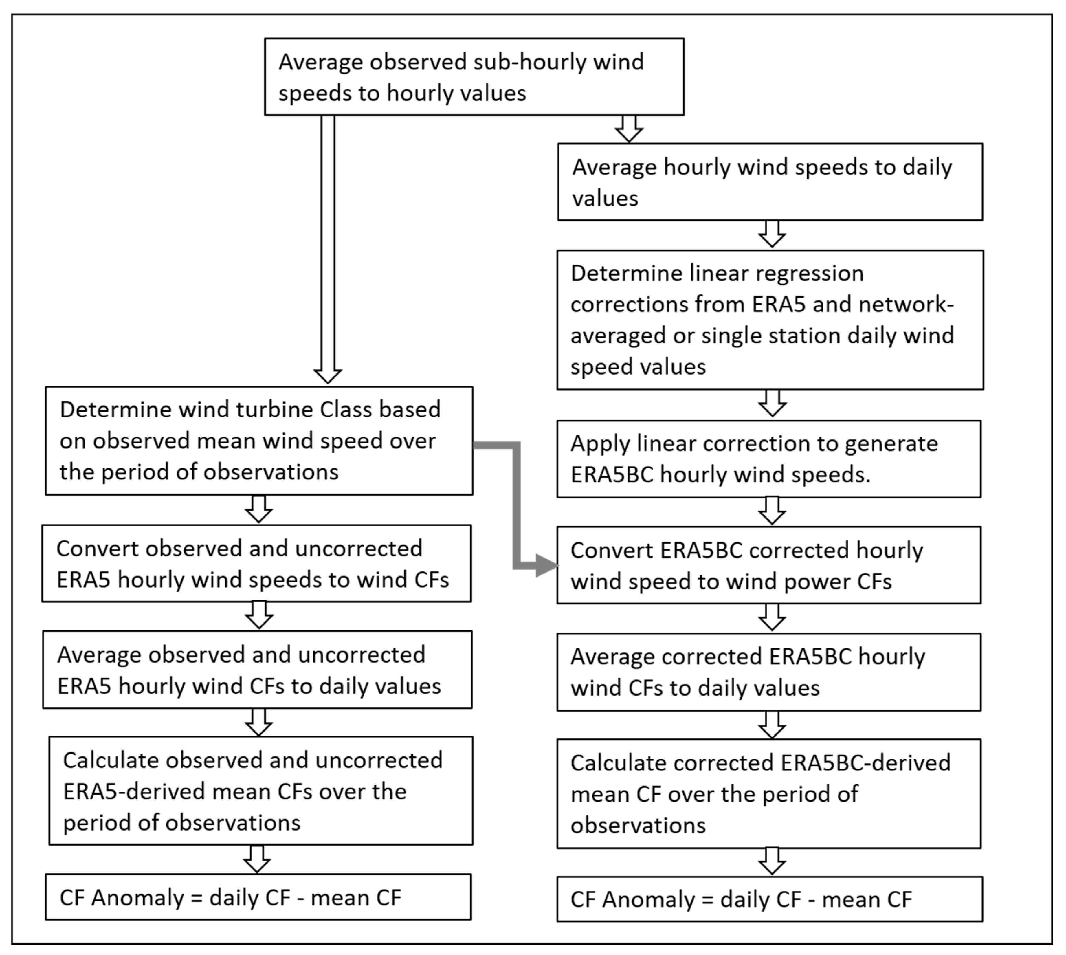
  • Processing Methods for Wind Power and Summary Statistics
Figure A9. Flow chart of processing steps to calculate daily observed, uncorrected ERA5-derived (left side boxes), and corrected ERA5-derived wind CFs (right side boxes) and CF anomalies. The same turbine class specification, based on the observed mean wind speeds for each observational data set, is used for the observations and ERA5. In the last step the anomalies are calculated independently for the observations, ERA5-derived, and corrected ERA5-derived CFs.
Energies 17 01667 g0a9
The WFIP1 tall-tower networks [57] consisted of 97 towers in the Northern Study Area (NSA) and 27 towers in the Southern Study Area (SSA), with measurement levels mostly between 60 and 80 m. Wind speeds from those towers were extrapolated to 100 m using a simple power law, with a power exponent value of 0.143. More complex stability-dependent methods were not used because the vertical extrapolations from 60 or 80 m to 100 m are relatively small; and second, as for the ARM-SGP site, the wind speed errors did not strongly vary across the diurnal cycle. All towers had two orthogonal or opposite booms, and speeds were calculated using the sensors on the booms least impacted by tower wakes, determined from hourly wind directions. For the Iowa Atmospheric Observatory set of two towers [58,59], we use observations from the A2 tower, which was further separated from existing wind turbines than tower A1, again using the upstream-oriented boom, and also blocking out some wind directions potentially affected by wind plants within 30 km. Also, for WFIP1, one sodar site (Ozona) was found to have its normalized mean bias more than double that of all the other WFIP sodars, and to have the opposite sign bias of those sodars. Comparing Ozona to a nearby site (Reagan, TX), the 100 m wind speed ERA5 values at the two sites are similar, but the Ozona observed mean speeds are more than 2 ms−1 smaller than the Reagan observations. Therefore, we have chosen to eliminate Ozona and only use 5 WFIP SSA sodars. We also did not use data from the Lubbock, TX sodar, as it was collocated with wind turbines at the Texas Tech University wind turbine testing facility, whose wakes could have affected the sodar measurements.
The WFIP2 data set [60,61] contained multiple sites that were in an area strongly influenced by gap flow winds that are channeled through the Columbia River Gorge. The Gorge is of sufficiently small scale that the ERA5 would have a difficult time resolving those gap winds. The study by Sharp and Mass [62] indicates that a model resolution of 3 km or better is likely needed to properly simulate these gap winds. Therefore, we eliminated 13 of the 22 sodar and lidar sites strongly influenced by the gap winds, leaving 9 outside of the Gorge area (Figure A10).
Figure A10. WFIP2 sites selected for inclusion in the ERA5 wind evaluation are shown as red circles, while sites within the area of extremely complex terrain associated with the Columbia Gorge that were not used are shown as blue open circles.
Energies 17 01667 g0a10
Many of the NYMesonet lidar stations [63] can also be affected by surface heterogeneity, as although all are situated on land, many of the stations are located very close to the coast, where the observations, ERA5 winds, or both, could be significantly influenced by the nearby ocean. Also, because the ERA5 uses a sub-grid-resolution tiled approach for specifying the surface roughness, in most cases for these coastal sites, the nearest ERA5 grid point would contain a mix of both land and ocean roughness lengths. As our goal is to characterize the ERA5 wind errors separately for land and ocean and to find corrections for each, we eliminated from consideration any NYmesonet lidar station that was within 15 km of the ocean or the Great Lakes, which is one half of the ERA5′s native grid resolution of ~31 km. This reduced the number of stations used from 17 down to 8. Also, some of the NYmesonet lidars as well as the Indiana lidar are mounted on buildings 8–13 m tall, and the height of the buildings was accounted for in determining the 100 m agl wind speed.
Figure A11. Summary statistics comparing the ERA5- (blue) and ERA5BC-derived (orange) wind CFs for each of the wind observation networks or single sites (1, WFIP2; 2, WFIP1-NSA-towers; 3, WFIP1-NSA-sodars; 4, WFIP1-SSA-towers; 5, WFIP1-SSA-sodars; 6, ARM-SGP; 7, Iowa; 8, NYSERDA; 9, Morro Bay; 10, Indiana; 11, NY Mesonet). (a) Normalized mean bias, (b) root-mean-squared error, (c) correlation coefficient, and (d) the ratio of the CF standard deviations from the ERA5 or ERA5BC to the observed, where the dashed line is the ideal value.
Energies 17 01667 g0a11

References

  1. Sharp, J. Meteorology 101: Meteorological Data Fundamentals for Power System Planning. Available online: https://www.esig.energy/weather-data-for-power-system-planning (accessed on 15 November 2023).
  2. Gualtieri, G. Analysing the uncertainties of reanalysis data used for wind resource assessment: A critical review. Renew. Sust. Energ. Rev. 2022, 167, 112741. [Google Scholar] [CrossRef]
  3. Kies, A.; Schyska, B.U.; Bilousova, M.; El Sayed, O.; Jurasz, J.; Stoecker, H. Critical review of renewable generation datasets and their implications for European power system models. Renew. Sustain. Energy Rev. 2021, 152, 111614. [Google Scholar] [CrossRef]
  4. Dörenkämper, M.; Olsen, B.T.; Witha, B.; Hahmann, A.N.; Davis, N.N.; Barcons, J.; Ezber, Y.; García-Bustamante, E.; González-Rouco, J.F.; Navarro, J.; et al. The Making of the New European Wind Atlas—Part 2: Production and evaluation. Geosci. Model. Dev. 2020, 13, 5079–5102. [Google Scholar] [CrossRef]
  5. Jourdier, B. Evaluation of ERA5, MERRA-2, COSMO-REA6, NEWA and AROME to simulate wind power production over France. Adv. Sci. Res. 2020, 17, 63–77. [Google Scholar] [CrossRef]
  6. Gualtieri, G. Reliability of ERA5 Reanalysis Data for Wind Resource Assessment: A Comparison against Tall Towers. Energies 2021, 14, 4169. [Google Scholar] [CrossRef]
  7. Brune, S.; Keller, J.D.; Wahl, S. Evaluation of wind speed estimates in reanalyses for wind energy applications. Adv. Sci. Res. 2021, 18, 115–126. [Google Scholar] [CrossRef]
  8. Pronk, V.; Bodini, N.; Optis, M.; Lundquist, J.K.; Moriarty, P.; Draxl, C.; Purkayastha, A.; Young, E. Can reanalysis products outperform mesoscale numerical weather prediction models in modeling the wind resource in simple terrain? Wind. Energy Sci. 2022, 7, 487–504. [Google Scholar] [CrossRef]
  9. Sheridan, L.M.; Krishnamurthy, R.; Gorton, A.M.; Shaw, W.J.; Newsom, R.K. Validation of Reanalysis-Based Offshore Wind Resource Characterization Using Lidar Buoy Observations. Mar. Technol. Soc. J. 2020, 54, 44–61. [Google Scholar] [CrossRef]
  10. Sheridan, L.M.; Krishnamurthy, R.; Medina, G.G.; Gaudet, B.J.; Gustafson, W.I.; Mahon, A.M.; Shaw, W.J.; Newsom, R.K.; Pekour, M.; Yang, Z.Q. Offshore reanalysis wind speed assessment across the wind turbine rotor layer off the United States Pacific coast. Wind. Energy Sci. 2022, 7, 2059–2084. [Google Scholar] [CrossRef]
  11. Urraca, R.; Huld, T.; Gracia-Amillo, A.; Martinez-de-Pison, F.J.; Kaspar, F.; Sanz-Garcia, A. Evaluation of global horizontal irradiance estimates from ERA5 and COSMO-REA6 reanalyses using ground and satellite-based data. Sol. Energy 2018, 164, 339–354. [Google Scholar] [CrossRef]
  12. Babar, B.; Graversen, R.; Boström, T. Solar radiation estimation at high latitudes: Assessment of the CMSAF databases, ASR and ERA5. Sol. Energy 2019, 182, 397–411. [Google Scholar] [CrossRef]
  13. Sianturi, Y.; Marjuki, M.; Sartika, K. Evaluation of ERAS and MERRA2 Reanalyses to Estimate Solar Irradiance Using Ground Observations over Indonesia Region. AIP Conf. Proc. 2020, 2223, 020002. [Google Scholar] [CrossRef]
  14. He, Y.Y.; Wang, K.C.; Feng, F. Improvement of ERA5 over ERA-Interim in Simulating Surface Incident Solar Radiation throughout China. J. Clim. 2021, 34, 3853–3867. [Google Scholar] [CrossRef]
  15. Khamees, A.S.; Khalil, S.A.; Morsy, M.; Hassan, A.H.; Rahoma, U.A.; Sayad, T. Evaluation of global solar radiation estimated from (ECMWF-ERA5) and validation with measured data over Egypt. Turk. J. Comp. Math. Educ. 2021, 12, 3996–4012. [Google Scholar]
  16. Tong, L.; He, T.; Ma, Y.C.; Zhang, X.T. Evaluation and intercomparison of multiple satellite-derived and reanalysis downward shortwave radiation products in China. Int. J. Digit. Earth 2023, 16, 1853–1884. [Google Scholar] [CrossRef]
  17. Wu, J.Y.; Fang, H.J.; Qin, W.M.; Wang, L.C.; Song, Y.; Su, X.; Zhang, Y.J. Constructing High-Resolution (10 km) Daily Diffuse Solar Radiation Dataset across China during 1982-2020 through Ensemble Model. Remote Sens. 2022, 14, 3695. [Google Scholar] [CrossRef]
  18. Jiang, H.; Yang, Y.P.; Bai, Y.Q.; Wang, H.Z. Evaluation of the Total, Direct, and Diffuse Solar Radiations From the ERA5 Reanalysis Data in China. IEEE Geosci. Remote Sens. 2020, 17, 47–51. [Google Scholar] [CrossRef]
  19. Li, Z.G.; Yang, X.; Tang, H. Evaluation of the hourly ERA5 radiation product and its relationship with aerosols over China. Atmos. Res. 2023, 294, 106941. [Google Scholar] [CrossRef]
  20. Mathews, D.; Gallachóir, B.O.; Deane, P. Systematic bias in reanalysis-derived solar power profiles & the potential for error propagation in long duration energy storage studies. Appl. Energy 2023, 336, 120819. [Google Scholar] [CrossRef]
  21. Qin, Y.; McVicar, T.R.; Huang, J.; West, S.; Steven, A.D.L. On the validity of using ground-based observations to validate geostationary-satellite-derived direct and diffuse surface solar irradiance: Quantifying the spatial mismatch and temporal averaging issues. Remote Sens. Environ. 2022, 280, 113179. [Google Scholar] [CrossRef]
  22. Hersbach, H.; Bell, B.; Berrisford, P.; Hirahara, S.; Horányi, A.; Muñoz-Sabater, J.; Nicolas, J.; Peubey, C.; Radu, R.; Schepers, D.; et al. The ERA5 global reanalysis. Q. J. R. Meteor. Soc. 2020, 146, 1999–2049. [Google Scholar] [CrossRef]
  23. Augustine, J.A.; DeLuisi, J.J.; Long, C.N. SURFRAD—A national surface radiation budget network for atmospheric research. B Am. Meteorol. Soc. 2000, 81, 2341–2357. [Google Scholar] [CrossRef]
  24. Augustine, J.A.; Hodges, G.B.; Cornwall, C.R.; Michalsky, J.J.; Medina, C.I. An update on SURFRAD—The GCOS Surface Radiation budget network for the continental United States. J. Atmos. Ocean. Technol. 2005, 22, 1460–1472. [Google Scholar] [CrossRef]
  25. Riihimaki, L.; Shi, Y.; Zhang, D. Data Quality Assessment for ARM Radiation Data (QCRAD1LONG). 1997-03-21 to 2020-05-25, Southern Great Plains (SGP) Facility. Atmospheric Radiation Measurement (ARM) User Facility. ARM Data Center, 1997. Available online: https://adc.arm.gov/discovery/#/results/instrument_code::qcrad1long/dataLevel::c2 (accessed on 23 March 2022). [CrossRef]
  26. Michalsky, J.J.; Gueymard, C.; Kiedron, P.; McArthur, L.J.B.; Philipona, R.; Stoffel, T. A proposed working standard for the measurement of diffuse horizontal shortwave irradiance. J. Geophys. Res.-Atmos. 2007, 112, D16112. [Google Scholar] [CrossRef]
  27. Holmgren, W.; Hansen, C.; Mikofski, M. pvlib Python: A python package for modeling solar energy systems. J. Open Source Softw. 2018, 3, 884. [Google Scholar] [CrossRef]
  28. Perez, R.; Ineichen, P.; Seals, R.; Michalsky, J.; Stewart, R. Modeling Daylight Availability and Irradiance Components from Direct and Global Irradiance. Sol. Energy 1990, 44, 271–289. [Google Scholar] [CrossRef]
  29. Jacobson, M.Z.; Jadhav, V. World estimates of PV optimal tilt angles and ratios of sunlight incident upon tilted and tracked PV panels relative to horizontal panels. Sol. Energy 2018, 169, 55–66. [Google Scholar] [CrossRef]
  30. Draxl, C.; Clifton, A.; Hodge, B.M.; McCaa, J. The Wind Integration National Dataset (WIND) Toolkit. Appl. Energy 2015, 151, 355–366. [Google Scholar] [CrossRef]
  31. Maraun, D. Bias Correction, Quantile Mapping, and Downscaling: Revisiting the Inflation Issue. J. Clim. 2013, 26, 2137–2143. [Google Scholar] [CrossRef]
  32. Polo, J.; Wilbert, S.; Ruiz-Arias, J.A.; Meyer, R.; Gueymard, C.; Súri, M.; Martín, L.; Mieslinger, T.; Blanc, P.; Grant, I.; et al. Preliminary survey on site-adaptation techniques for satellite-derived and reanalysis solar radiation datasets. Sol. Energy 2016, 132, 25–37. [Google Scholar] [CrossRef]
  33. Harmsen, E.W.; Tosado-Cruz, P.; Mecikalski, J.R. Calibration of selected pyranometers and satellite derived solar radiation in Puerto Rico. Int. J. Renew. Energy Technol. 2014, 5, 43–54. [Google Scholar] [CrossRef]
  34. Polo, J.; Martín, L.; Vindel, J.M. Correcting satellite derived DNI with systematic and seasonal deviations: Application to India. Renew. Energy 2015, 80, 238–243. [Google Scholar] [CrossRef]
  35. Bender, G.; Davidson, F.; Eichelberger, F.; Gueymard, C.A. The road to bankability: Improving assessments for more accurate financial planning. In Proceedings of the Solar 2011 Conference American Solar Energy Society, Raleigh, NC, USA, 19 May 2011. [Google Scholar]
  36. Gueymard, C.A.; Gustafson, W.T.; Bender, G.; Etringer, A.; Storck, P. Evaluation of procedures to improve solar resource assessments: Optimum use of short-term data from a local weather station to correct bias in long-term satellite derived solar radiation time series. In Proceedings of the World Renewable Energy Forum, Denver, CO, USA, 13–17 May 2012. [Google Scholar]
  37. Schumann, K.; Beyer, H.G.; Chhatbar, K.; Meyer, R. Improving satellite-derived solar resource analysis with parallel ground-based measurements. In Proceedings of the ISES Solar World Congress, Kasel, Germany, 28 August–2 September 2011. [Google Scholar]
  38. Ruiz-Arias, J.A.; Quesada-Ruiz, S.; Fernández, E.F.; Gueymard, C.A. Optimal combination of gridded and ground-observed solar radiation data for regional solar resource assessment. Sol. Energy 2015, 112, 411–424. [Google Scholar] [CrossRef]
  39. Wood, A.W.; Maurer, E.P.; Kumar, A.; Lettenmaier, D.P. Long-range experimental hydrologic forecasting for the eastern United States. J. Geophys. Res.-Atmos. 2002, 107, ACL 6-1–ACL 6-15. [Google Scholar] [CrossRef]
  40. Wood, A.W.; Lettenmaier, D.P. A test bed for new seasonal hydrologic forecasting approaches in the western United States. B Am. Meteorol. Soc. 2006, 87, 1699–1712. [Google Scholar] [CrossRef]
  41. Piani, C.; Haerter, J.O.; Coppola, E. Statistical bias correction for daily precipitation in regional climate models over Europe. Theor. Appl. Clim. 2010, 99, 187–192. [Google Scholar] [CrossRef]
  42. Hopson, T.M.; Webster, P.J. A 1-10-Day Ensemble Forecasting Scheme for the Major River Basins of Bangladesh: Forecasting Severe Floods of 2003-07. J. Hydrometeorol. 2010, 11, 618–641. [Google Scholar] [CrossRef]
  43. Gudmundsson, L.; Bremnes, J.B.; Haugen, J.E.; Engen-Skaugen, T. Technical Note: Downscaling RCM precipitation to the station scale using statistical transformations—A comparison of methods. Hydrol. Earth Syst. Sci. 2012, 16, 3383–3390. [Google Scholar] [CrossRef]
  44. Costoya, X.; Rocha, A.; Carvalho, D. Using bias-correction to improve future projections of offshore wind energy resource: A case study on the Iberian Peninsula. Appl. Energy 2020, 262, 114562. [Google Scholar] [CrossRef]
  45. Campos, R.M.; Gramcianinov, C.B.; de Camargo, R.; Dias, P.L.D. Assessment and Calibration of ERA5 Severe Winds in the Atlantic Ocean Using Satellite Data. Remote Sens. 2022, 14, 4918. [Google Scholar] [CrossRef]
  46. Cannon, A.J.; Sobie, S.R.; Murdock, T.Q. Bias Correction of GCM Precipitation by Quantile Mapping: How Well Do Methods Preserve Changes in Quantiles and Extremes? J. Clim. 2015, 28, 6938–6959. [Google Scholar] [CrossRef]
  47. Augustine, J.A.; Capotondi, A. Forcing for Multidecadal Surface Solar Radiation Trends Over Northern Hemisphere Continents. J. Geophys. Res.-Atmos. 2022, 127, e2021JD036342. [Google Scholar] [CrossRef]
  48. MacDonald, A.E.; Clack, C.T.M.; Alexander, A.; Dunbar, A.; Wilczak, J.; Xie, Y.F. Future cost-competitive electricity systems and their impact on US CO emissions. Nat. Clim. Chang. 2016, 6, 526–531. [Google Scholar] [CrossRef]
  49. Phadke, A.; Paliwal, U.; Abhyankar, N.; McNair, T.; Paulos, B.; Wooley, D.; O’Connell, R. The 2035 Report: Plummeting Solar, Wind, and Battery Costs Can. Accelerate Our Clean. Electricity Future; Goldman School of Public Policy, University of California Berkeley: Berkeley, CA, USA, 2020. [Google Scholar]
  50. Brown, P.; Botterud, A. The Value of Inter-Regional Coordination and Transmission in Decarbonizing the US Electricity System. Joule 2021, 5, 115–134. [Google Scholar] [CrossRef]
  51. Sengupta, M.; Xie, Y.; Lopez, A.; Habte, A.; Maclaurin, G.; Shelby, J. The National Solar Radiation Data Base (NSRDB). Renew. Sust. Energy Rev. 2018, 89, 51–60. [Google Scholar] [CrossRef]
  52. Shippert, T.; Newsom, R.; Riihimaki, L.; Zhang, D. Doppler Lidar Horizontal Wind Profiles (DLPROFWIND4NEWS), Southern Great Plains (SGP) Facility; Atmospheric Radiation Measurement (ARM) User Facility; ARM Data Center, 2010. Available online: https://adc.arm.gov/discovery/#/results/instrument_code::dlprofwind4news/dataLevel::c1 (accessed on 22 March 2022). [CrossRef]
  53. Jensen, M.P.; Toto, T.; Troyan, D.; Ciesielski, P.E.; Holdridge, D.; Kyrouac, J.; Schatz, J.; Zhang, Y.; Xie, S. The Midlatitude Continental Convective Clouds Experiment (MC3E) sounding network: Operations, processing and analysis. Atmos. Meas. Technol. 2015, 8, 421–434. [Google Scholar] [CrossRef]
  54. Staffell, I.; Pfenninger, S. Using bias-corrected reanalysis to simulate current and future wind power output. Energy 2016, 114, 1224–1239. [Google Scholar] [CrossRef]
  55. DNV-GL. NYSERDA Floating LiDAR Buoy Data. Available online: https://oswbuoysny.resourcepanorama.dnv (accessed on 13 September 2023).
  56. Bodini, N.; Lundquist, J.K.; Moriarty, P. Wind plants can impact long-term local atmospheric conditions. Sci. Rep. 2021, 11, 22939. [Google Scholar] [CrossRef]
  57. Wilczak, J.; Finley, C.; Freedman, J.; Cline, J.; Bianco, L.; Olson, J.; Djalalova, I.; Sheridan, L.; Ahlstrom, M.; Manobianco, J.; et al. The Wind Forecast Improvement Project (WFIP) A Public-Private Partnership Addressing Wind Energy Forecast Needs. Bull. Am. Meteorol. Soc. 2015, 96, 1699–1718. [Google Scholar] [CrossRef]
  58. Takle, E.S.; Rajewski, D.A.; Purdy, S.L. The Iowa Atmospheric Observatory: Revealing the Unique Boundary Layer Characteristics of a Wind Farm. Earth Interact. 2019, 23, 1–27. [Google Scholar] [CrossRef]
  59. Rajewski, D.A.; Takle, E.S.; VanLoocke, A.; Purdy, S.L. Observations Show That Wind Farms Substantially Modify the Atmospheric Boundary Layer Thermal Stratification Transition in the Early Evening. Geophys. Res. Lett. 2020, 47, e2019GL086010. [Google Scholar] [CrossRef]
  60. Shaw, W.J.; Berg, L.K.; Cline, J.; Draxl, C.; Djalalova, I.; Grimit, E.P.; Lundquist, J.K.; Marquis, M.; McCaa, J.; Olson, J.B.; et al. The Second Wind Forecast Improvement Project (WFIP2): General Overview. Bull. Am. Meteorol. Soc. 2019, 100, 1687–1699. [Google Scholar] [CrossRef]
  61. Wilczak, J.M.; Stoelinga, M.; Berg, L.K.; Sharp, J.; Draxl, C.; McCaffrey, K.; Banta, R.M.; Bianco, L.; Djalalova, I.; Lundquist, J.K.; et al. The Second Wind Forecast Improvement Project (WFIP2): Observational Field Campaign. Bull. Am. Meteorol. Soc. 2019, 100, 1701–1723. [Google Scholar] [CrossRef]
  62. Sharp, J.M.; Mass, C. Columbia Gorge gap flow—Insights from observational analysis and ultra-high-resolution simulation. Bull. Am. Meteorol. Soc. 2002, 83, 1757–1762. [Google Scholar] [CrossRef]
  63. Brotzge, J.A.; Wang, J.; Thorncroft, C.D.; Joseph, E.; Bain, N.; Bassill, N.; Farruggio, N.; Freedman, J.M.; Hemker, K.; Johnston, D.; et al. A Technical Overview of the New York State Mesonet Standard Network. J. Atmos. Ocean. Technol. 2020, 37, 1827–1845. [Google Scholar] [CrossRef]
Figure 1. NOAA SURFRAD (blue circles) and SOLRAD (red circles) observation sites, and the DOE ARM-SGP network region (green square). The Hanford site was not included in the analysis due to frequent missing data.
Energies 17 01667 g001
Figure 2. ERA5 versus SURFRAD PSU daily averaged irradiances. (a) GHI; (b) DHI; (c) DNI; (d) DIRhor. Orthogonal least squares linear fits are shown as the red lines, with the corresponding slope and intercept (Int), correlation coefficient (Cor), bias, and normalized mean bias (NMB) given in each panel.
Energies 17 01667 g002
Figure 3. Annual cycle of daily mean solar capacity factor at the SURFRAD PSU site averaged over the time period 1998–2020, for the SURFRAD observations (red), and from the time-matched ERA5 (blue), with their corresponding four-harmonic fits (SURFRAD, yellow; ERA5, cyan), for the uncorrected ERA5 (a) and corrected ERA5BC (b); scatter plots of ERA5 (c) and ERA5BC (d) vs. SURFRAD PSU daily solar CF values. Orthogonal least squares linear fits are shown as the red lines and values are given as in Figure 2.
Energies 17 01667 g003
Figure 4. Solar CF histograms for the SURFRAD PSU site (orange) and ERA5 (blue), for annual (a), DJF (b), and JJA (c) periods, for the original ERA5 derived values (ac), and for ERA5BC (df).
Energies 17 01667 g004
Figure 5. Intensity–duration curves of the largest normalized solar capacity factor anomalies (positive and negative) as a function of duration, for the uncorrected ERA5 (blue curves) and the SURFRAD PSU observations (red curves), using data for all months of the year, for years 1998–2020.
Energies 17 01667 g005
Figure 6. Intensity–duration diagrams as in Figure 5, except at each of the SURFRAD/SOLRAD sites and for the ARM aggregate. The abscissa on each panel is the duration from 1–90 days, and the ordinate is CF anomaly as a percent, from −100 to +100. Sites corresponding to those in Figure 1 are Seattle (SEA), Fort Peck (FPK), Sioux Falls (SXF), Penn State University (PSU), Salt Lake City (SLC), Bismark (BIS), Madison (MSN), Sterling (STE), Desert Rock (DRA), Table Mountain (TBL), Bondville (BON), Albuquerque (ABQ), ARM-SGP aggregate (ARM-agg), and Goodwin Creek (GWN).
Energies 17 01667 g006
Figure 7. As in Figure 6, except for the QM-corrected ERA5 (ERA5BC).
Energies 17 01667 g007
Figure 8. Intensity–duration curves over the full annual period derived from 13 SURFRAD/SOLRAD sites and averaged over those sites (red curves); from the corresponding uncorrected ERA5 (blue lines); from the 13-site average of the closest NSRDB grid cells corresponding to each of the SURFRAD/SOLRAD sites (green dotted lines); and from the 13-site average using averages of an 8 × 8 array of NSRDB points surrounding each SURFRAD/SOLRAD site (purple dashed line).
Energies 17 01667 g008
Figure 9. Annual cycle (a) and diurnal cycle (b) of uncorrected ERA5 100 m wind speed for the aggregate of the 4 ARM-SGP sites for the time period of 2016–2021.
Energies 17 01667 g009
Figure 10. Scatter plots of observed and corresponding uncorrected ERA5-derived daily wind speeds or aggregate wind speeds for 11 different wind data sets: (a) WFIP2 non-Gorge sodars and lidars; (b) Iowa Atmospheric Observatory tower; (c) NY mesonet lidars; (d) WFIP1 NSA towers; (e) WFIP1 NSA sodars; (f) Indiana lidar; (g) WFIP1 SSA towers; (h) WFIP1 SSA sodars; (i) ARM-SGP lidars; (j) Morro Bay buoy lidar; and (k) NYSERDA buoy lidars. Red lines show orthogonal least squares linear fits. Panel titles display the slope, intercept, correlation coefficient, bias, and normalized mean bias as a percent.
Energies 17 01667 g010
Figure 11. Annual cycles of wind CF derived from the uncorrected ERA5 (a) and ERA5BC (b). The 6-year mean for each day of the year is shown for the average of 4 ARM-SGP lidars (red) and the ERA5 or ERA5BC (blue). Corresponding four-harmonic fits are shown for the lidar observations (yellow) and the ERA5 or ERA5BC (cyan). Histograms of derived wind CF from the observations (orange) and uncorrected ERA5 (blue) (c), and for ERA5BC (d). Scatter plots of ERA5-derived versus observed CF values for the uncorrected ERA5 (e) and ERA5BC (f). Intensity–duration curves of capacity factor anomalies as a percent of the annual mean capacity factor, as a function of duration, for the observations (red) and ERA5 (g) or ERA5BC (h).
Energies 17 01667 g011
Figure 12. Intensity–duration curves of the largest normalized wind capacity factor anomalies (positive and negative) as a function of duration, for the uncorrected ERA5 (blue curves) and the observations (red curves), using data for all months of the year, for years of observations available as indicated. The abscissa on each panel is the duration from 1–90 days, and the ordinate is normalized CF anomaly as a percent, from −100 to +100.
Energies 17 01667 g012
Figure 13. As in Figure 12, except for the ERA5BC.
Energies 17 01667 g013
Figure 14. ERA5 mean 100 m normalized wind speed bias (NMB) (ERA5—observations) at each of the wind observation locations. The two larger circles represent aggregate biases from the WFIP NSA region (97 towers) and the SSA region (27 towers).
Energies 17 01667 g014
Disclaimer/Publisher’s Note: The statements, opinions and data contained in all publications are solely those of the individual author(s) and contributor(s) and not of MDPI and/or the editor(s). MDPI and/or the editor(s) disclaim responsibility for any injury to people or property resulting from any ideas, methods, instructions or products referred to in the content.

