Electric Vehicle Routing Problem with an Enhanced Vehicle Dispatching Approach Considering Real-Life Data

Abstract

Although the EVRP (Electric Vehicle routing problem) has promising results on the environmental scale, its implementation has proved challenging. The difficulty of the EVRP resides in the limited driving range of the electric vehicles, combined with the significant charging time. While the charging cost is less than the cost of fuel, this charge time adds to the overall travel time and may overlap with customers’ time windows. All these factors increased the computational time exponentially and resulted in the need to overlook some constraints such as traffic congestion, road conditions, weather impact on energy consumption, and driving style, to name a few, in order to speed up execution time. While this method proved effective in accelerating the process of the EVRP, it did, however, render the approach unrealistic, as it steered far from real-life settings and made the approach unpredictable when facing dynamic and changing parameters. In this paper, we try to remedy this issue by proposing an approach in which we try to replicate real-life parameters such as heterogenous fleets, energy consumption, and infrastructure data. The objective of our approach was to minimize the total travel time, travel distance, energy consumed, and the number of vehicles deployed. To solve this problem, we propose a three-stages approach, in which the first stage consists of a newly developed dispatching approach where customers are assigned to vehicles. The second stage uses the genetic algorithm to find a set of optimal paths, and, finally, in the third stage, charging stations are inserted in the selected paths. Upon testing our approach on Solomon’s instances, our approach proved effective in finding optimal solutions in a reasonable time for five- to fifteen-customer datasets. However, when trying to solve larger datasets, the approach was slowed down by the extreme number of constraints it had to satisfy.

1. Introduction

With the dawn of the industrial revolution in the 18th century, and the race to score the leading place in the international market, countries in the four corners of the globe invested in, among other things, larger fleets to strengthen their logistics performances. For decades, steam- or gasoline-propelled vehicles of all types were roaming seas, lands, and skies, ensuring a wide distribution of goods. The objective for industries was to reach as many markets as possible and ensure the widest spread of their products. Accordingly, the costs invested in distribution grew more expensive. For instance, the more customers that were served, the more distance was travelled, which translated into more fuel to acquire. As a preventive measure, suppliers concentrated their focus on ensuring an optimal use of resources, such as the number of vehicles deployed, energy, and time, amongst others, while preserving the ability to serve as many customers as possible. This required good management of transportation means, formally known as the VRP (Vehicule Routing Problem). This problem was first introduced in 1959 [1], and it was inspired by the TSP (Travelling Salesperson/Salesman Problem) [1], which aims to find the optimal path to serve a set of customers, once each, at the lowest cost possible.

The focus on electric vehicles led to the birth of the eco-friendly version of the VRP, the EVRP. Following in the footsteps of the VRP, the EVRP aims to find the optimal set of routes that will allow a fleet of electric vehicles to serve a set of customers. Several works throughout the years tried to tackle the EVRP riddle but were faced with some challenges. The difficulty of the EVRP resides in the fact that electric vehicles require careful and precise route planification to avoid depleting the batteries. Furthermore, the existing infrastructure is yet to be ready for a full switch to electric vehicles, since existing charging stations are still few and far between [2,3,4]. Additionally, similarly to the VRP, once the number of customers exceeds a certain threshold, it becomes computationally difficult to solve the EVRP in a reasonable time. Finally, it is complicated to mimic real-life settings during simulations, which is the one of the reasons why most VRP (and EVRP) approaches ignored most settings. Although this option reduces simulation time, it is difficult to rely on it in real life, as the behavior of the approach becomes unpredictable.

In this paper, we present a new method of solving the EVRP, with time windows and capacitated heterogenous vehicles in real-life settings. Our approach emulates the classic EVRP approach, which aims to serve a set of customers using a fleet of vehicles at the lowest cost possible. The term ‘cost’ changes its definition according to the approach considered. For instance, cost can refer to the total distance, the total time of travel, or the total monetary costs dispensed throughout the routing process amongst others. However, in our approach, we consider four costs: total elapsed time, travelled distance, consumed energy, and number of vehicles deployed. The first three terms represent, respectively, the sum of the time, distance, and energy generated by each vehicle from the start to the end of its tour. Our objective is to minimize these four components, with the priority being the total travelled time, while creating a real-life-like approach that can adapt to any scenario at hand. In our approach, we try to mimic day-to-day settings such as road topography, driver’s behavior, fluctuating waiting times, difficult weather, and speed limitations, among other factors. However, the extreme number of factors impacting the approach renders the resolution difficult, since, whichever algorithm we choose, the approach will still have to abide by several rules which slow it down. To this end, we propose a three-stage approach to solve the EVRP, considering our scenario: dispatching, an optimal path search conducted using the genetic algorithm, and station insertion.

Therefore, this paper will be organized as follows: first, there is a problem description, in which we summarize some of the related works, in Section 2. Second, we will provide a detailed mathematical formulation of our model in Section 3. Third, we will explain the approach used to solve this model in Section 4. Fourth, we will describe the process and the parameters considered for simulation in Section 5. Fifth, the results of our simulation will be analyzed and discussed in Section 6. Finally, we will summarize our reflections in the conclusion.

2. Problem Description

The main factor that makes the difference between all works concerning the EVRP is not necessarily the methodology used to solve it, but mainly the scenarios considered. For instance, in [5], authors considered the routing of shared autonomous and identical vehicles during traffic congestion. Their approach took into consideration the factors of distance, speed, and vehicle weight, and evaluated their effect on vehicle capacity, time window, and battery level. While computing energy consumption, they integrated the power loss by the vehicle as well. To solve their version of the EVRP, they resorted to the adaptive large neighborhood search. Although their approach saved up to a quarter of the total costs, by focusing on speed and the optimization of departure time, it would strongly benefit from real-time traffic data, to adapt to the user’s requests. To keep up with unexpected events, [6] suggested a new approach to adapt to unforeseen changes in an already planned path. Their approach was to decide when and where to skip nodes, using a crowd learning particle swarm optimization algorithm. Their solution proved effective in solving large-scale instances, but only when the loading time was fixed, and when the fleet was homogenous, for instance. Weather was also another factor that was ignored in their approach.

While energy consumption might be a key factor in the deployment of electric vehicles, [7] chose to focus on other factors in their approach. In their work, they considered a very challenging version of the EVRP, in which they considered time windows and mixed backhauls, and, to solve it, they used a combination of three approaches: genetic operation, the selection of individuals regardless of their feasibility, and road information updates. To test their approach, they subjected it to instances of variant sizes that reached up to 200 customers and 40 charging stations. Compared to similar approaches, their methodology yielded an acceptable performance. Some works, like that of [8], chose to use deep reinforcement learning to solve the EVRP. In their work, they used electric vehicles to provide customers with energy, which implies that they had to focus on energy from two perspectives: vehicle consumption and customer needs. They included solar irradiance in the energy consumption calculation and applied it to the Chicago area. Upon running the approach in dynamic conditions, it outperformed three heuristic algorithms: the genetic algorithm, particle swarm optimization, and the artificial fish swarm algorithm. However, the vehicles used were dependent on one another, and unable to make decisions on their own.

What makes the EVRP difficult is its inability to mimic real-life settings. In any simulation, settings are either assumed and therefore fixed beforehand, or completely ignored. Neither case reflects what really happens when an approach is put to the test in a dynamic and changing environment. Therefore, several works tried to incorporate this dynamic aspect to their EVRP approach, to create the flexibility that conventional approaches lacked. For instance, the work in [9] considered demand uncertainty in their approach, which dealt with the electric vehicle routing problem with energy consumption that depends on weight. Their methodology consisted of a large neighborhood search that was reinforced with an adaptive mechanism that set the required selection operator to avoid local optima. Simulations were run on an adapted version of pollution routing problem instances, with a maximum of 100 customers. The results indicated that the approach was capable of making a compromise between cost and risk by operating on uncertain parameters. The same heuristic was deployed in [10] for their EVRP approach, with a partial recharge policy. A fuzzy simulation approach was employed as well, to boost the aforementioned algorithm and symbolize the uncertainties of service time, battery energy consumption, and travel time. In this approach, simulations were conducted on 34 randomly generated instances of up to 200 customers, eight charging stations, using vehicles of 100 load capacity and 150 driving range. Compared to other heuristics, the proposed approach had a better convergence rate, a better local search ability, and found the best solution. The approach could, however, be improved by considering heterogenous fleets and flexible speed, as well as waiting time, which was considered in [11]. In that work, they devised a time-dependent waiting time function that followed a Poisson distribution, where waiting time depended on whether the charger at the charging station was available or not. Once more, adaptive large neighborhood search was deployed to solve the proposed approach using Solomon’s instances [12], by treating fuel stations as charging stations. The proposed approach outperformed CPLEX, which is an optimization problems solver, in terms of computational time and solution quality. It was proven that, when waiting times were long, the number of vehicles increased. However, customer’s time windows did not impact the final solutions. Solomon’s instances were also used in [13], where the authors focused on the monetary cost of energy in a dynamic situation. They used a combination of variable neighborhood search and tabu search to solve their approach. It was proven that the higher the number of vehicles deployed was, the less energy was consumed, but it did not necessarily improve the routing. In other words, when more vehicles are used, the path of each vehicle becomes shorter, hence the energy consumption reduction, but that doesn’t mean that the routing solution is optimal. The approach is also affected by energy prices and time windows amongst others.

Heterogenous fleets were discussed in a work where the fleet was composed of autonomous electric vehicles [14]. The approach considered energy consumption, charging/recharging cost, and driver’s cost, and used variable neighborhood search, along with large neighborhood search. Their work confirmed that a heterogenous fleet reduced the operational costs.

Aside from waiting times, another time-consuming factor that impacts the overall routing experience is the traffic conditions [15,16,17]. It is only logical that, when traffic is congested, vehicles require more time to move from one point to another, which imposes one of the two following options: (a) abide by traffic rules, thus increasing travel time, or (b) choose a different path with less traffic. The second option is not always possible, especially during rush hour when most streets are jammed. Additionally, it makes the EVRP more complicated, as the change in path requires a new planification to avoid depleting the batteries. That leaves us with the first option, which leads to higher costs in terms of time and energy consumed. This requires a prior knowledge of traffic conditions at the time of planning, but this is not always achievable. To solve this dilemma, some works, for example [18], resorted to randomly generated traffic data, along with speed scenarios to mimic real-life scenarios. Using the branch-and-cut-and-price algorithm, their approach was able to solve the EVRP with up to 133 customers, with reasonable results.

In another work, [19], the authors used an elitist version of the genetic algorithm, coupled with an improved neighbor routing method. This method ensured the selection of the current customer’s nearest neighbor. The approach was simulated using 25 randomly distributed customers, and it was proven that the approach converged faster due to the elitist factor deployed. However, this was only the case with randomly distributed instances in a static scenario. The approach did not include the dynamicity of charging time and other external factors that could impact the routing experience, such as traffic for instance.

What sets our approach apart is that most works generally disregarded energy consumption in favor of other factors, mainly time windows, charging style, and fleet characteristics. Although this approach alleviated the problem’s complexity and greatly boosted computational time, they still cannot be considered an accurate representation of real-life settings, where several of the following factors apply: traffic, weather, energy consumption of auxiliaries on board, and speed limits, amongst others.

In a scenario in which a warehouse is assigned goods delivery to a set of customers, using a fleet of heterogenous vehicles, we aim to find the optimal set of routes that will allow for an optimal distribution of goods at the lowest cost possible. In our version of the EVRP, we include time of travel, covered distance, consumed energy, and number of vehicles deployed in the definition of cost. Therefore, we aim to provide a solution that covers the four aspects of the optimal cost: time, distance, energy, and number of vehicles. In case it proves difficult to minimize all four parameters at once, a compromise can to be made by focusing on time of travel in favor of the rest of the parameters. If the time of travel of two paths is identical, the travelled distance becomes the decision factor, followed by the energy consumed.

Costs to be considered are impacted by several factors, mainly speed, infrastructure (speed limit, traffic, road topography, etc.), wasted energy (aggressive driving, for instance), and non-added value time such as parking time, waiting time (at the charging station and at the customer), and charging time itself.

The warehouse in charge of providing the goods is supposed to have a specified schedule limited to 24 h. All delivery operations are to be conducted within this time window.

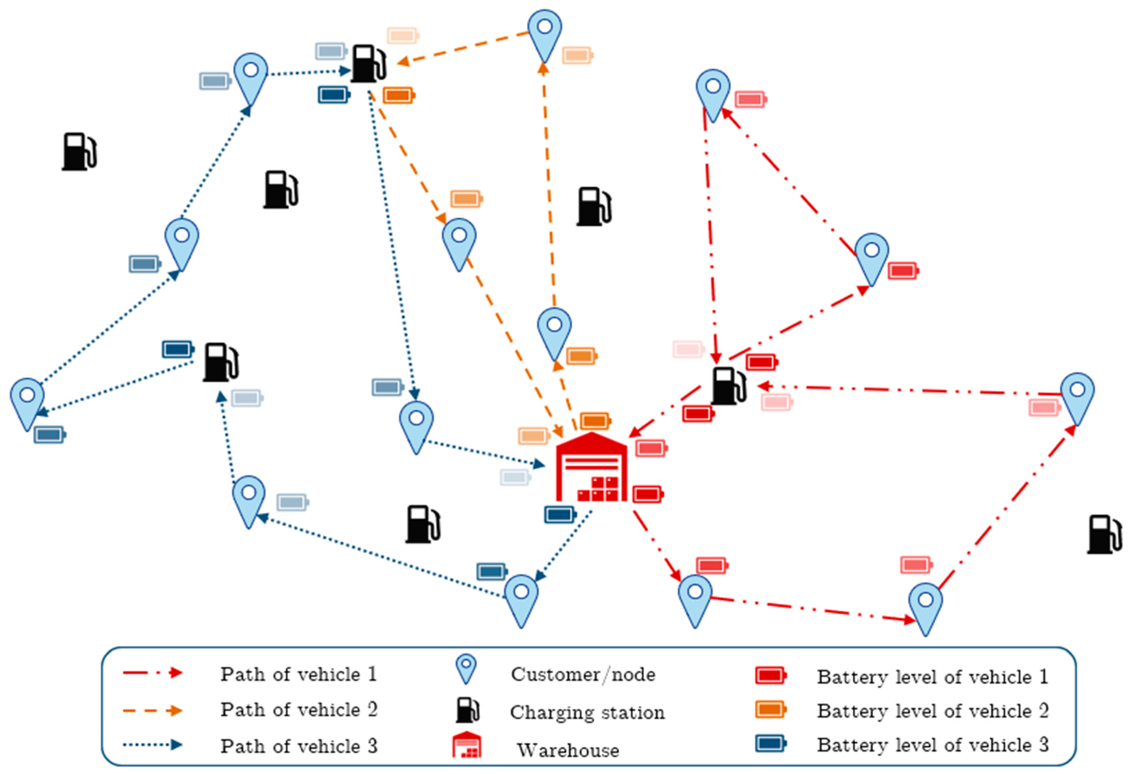
The desired output of any EVRP is to assign the optimal set of paths to a fleet of vehicles. Those assigned paths should ensure an optimal distribution of goods to a set of customers. Figure 1 is an example of a scenario in which we used three vehicles to move between the warehouse and the 14 customers that need to be served. Each vehicle has its own set of customers to serve, and can stop to recharge along the way, when and if necessary. Not all charging stations must be visited, but the same charging station can be used by more than one vehicle (vehicle 2 and vehicle 3 share a charging station), or by the same vehicle several times (vehicle 1 passes by the same charging station twice).

3. Mathematical Formulation

We use $G=\{P_0,C_t U S_t,S_{t\prime }, E\}$ as a graph that represents the main actors in our approach, with the customers P₀ and C_t, to which we added the warehouse, denoted as $0$, stations ($S_t$), and the edges $E=\left\{\right(i,j\left)\right|j,i \in P_0,C_t U S_t,S_{t\prime }, \vartheta \}$ that connect them all. $S_{t\prime }$ is a copy of the ensemble $S_t$ of stations, which is $\beta$, to allow vehicles multiple visits to the same station. $\theta$ is the ensemble of speeds between edges.

Let $C_t$ $=\{1\dots C\}$ be a set of geographically scattered customers, $V_h=\{1\dots N\}$ a fleet of heterogenous vehicles, and $S_t=\{1\dots S\}$ several charging stations and their duplicates $S_{t\prime }=\{1\dots S\prime \}$. Each arc $(i,j)$ is assigned a specific velocity (i.e., speed) $\mathit{\vartheta }={\sum }_{\left(i,j\right)\in G} V_{ij}$, which represents the speed needed to drive from $i$ to $j$ (and from $j$ to $i$ as well). The vehicles, being heterogenous, are represented by their driving range ${Dr}_y (\forall y \in V_h)$, load capacity ${Cap}_y (\forall y \in V_h)$, and battery capacity ${Bat}_y (\forall y \in V_h)$.

3.1. Objective Function

Our approach builds on the classic EVRP while focusing on the overall time of travel and aiming to minimize it within reason, without tampering with the efficiency of the approach. The objective function is thus expressed as follows:

$$min\left(\sum _{\left(i,j\right)\in G,, y\in V_h}{T}_{\mathit{ijy}}.x_{ij}+\sum _{\left(i,j\right)\in G,, y\in V_h}{\mathit{Dist}}_{\mathit{ijy}}.x_{ij}+\sum _{\left(i,j\right)\in G, y\in V_h}{E}_{\mathit{ijy}}.x_{ij}.{\mathsf{\beta }}_y+{\displaystyle \sum _{\left(i,j\right)\in G, y\in V_h}}{\mathsf{\beta }}_y{.x}_{ij} \right)$$

(1)

The objective function focuses on minimizing the sum of the following four factors: time of travel, total travelled distance, energy consumed during the travel, and number of vehicles deployed, where $x_{ij}$ is a binary variable that is set as 1 if the edge that connects node $i$ to $j (\forall i,j \in G) is used, 0 otherwise$, ${\mathsf{\beta }}_y$ is a binary variable that is set as 1 if the vehicle $y (\forall y\in V_h)$ is used, 0otherwise, $T_{ijy}$ is the time needed to drive from $i$ to $j (\forall i,j \in G)$ using vehicle $y$ $(\forall y\in V_h)$, ${Dist}_{ijy}$ is the distance travelled from $i$ to $j (\forall i,j \in G$) using vehicle $y$ $(\forall y\in V_h)$, and $E_{ijy}$ is the energy consumed by vehicle $y$ $(\forall y\in V_h)$ when driving from $i$ to $j (\forall i,j \in G)$.

The objective function is subject to several constraints, which are detailed in the following section.

3.2. Constraints

3.2.1. Distance and Speed Constraints

The final output of our approach is established to be a set of paths connecting a number of customers and charging stations to the warehouse, which are paths assigned to each vehicle. It is judicious to mention that not all vehicles have to be deployed and not all paths should pass by a (or several) charging stations.

As the weather impacts the driving range [1], we use the variable temp, which expresses the current temperature surrounding the vehicle. If that temperature is below 15 °C, the driving range decreases by 28%; otherwise, it stays intact. While the total distance travelled by a vehicle can largely exceed its driving range, the distance driven by a vehicle y connecting two nodes $i$ and $j$, denoted $Dis{t}_{ijk}$, can never exceed the vehicle’s remaining driving range ${RD}_y (\forall i \in V_h)$, which is insured by constraint (3).

$$\left\{\begin{array}{c}{Dist}_{ijy}<{RD}_y \left(\forall y\in Vh\right) , if temp \ge 15 °\mathrm{C}\\ {Dist}_{ijy}<{RD}_y\times 0.72 \left(y\forall \in Vh\right) , otherwise\end{array} \forall y\in Vh\right.$$

(2)

This constraint ensures that the vehicle’s remaining driving range ${RD}_y (\forall i \in V_h)$ is always larger than the distance needed to reach the next node; this is to avoid stopping midway.

Speed along each arc is fixed beforehand based on road conditions, traffic congestion, and road topography. Constraint (3) ensures that the speed $V_{ij} (\forall i,j \in G)$ at which a driver drives their vehicle along arc $(i,j) (\forall i,j \in G)$ does not surpass the designated speed $u$, $(\forall u \in \theta ).$

$${Dist}_{ijy}<{RD}_y\times \mathrm{T} (\forall \mathrm{y}\in \mathrm{V}\mathrm{h})$$

(3)

At the same time, along with driving style, speed affects energy consumption. Equation (4) portrays the formula β, which is used to calculate the energy consumption of every arc $(i,j) (\forall i,j \in G)$, taking into consideration the driving style, the speed of that arc, and the vehicle characteristics, as follows:

$$0\le {\mathrm{V}}_{\mathrm{i}\mathrm{j}}\le \mathrm{u},\forall \mathrm{i},\mathrm{j}\in \mathrm{G},\forall \mathrm{u}\in \mathsf{\theta }$$

(4)

where $P_{tr}$ is the energy of traction, provided by the batteries to propel the vehicle, and it is the sum of the following four main components: rolling resistance $P_{roll}$, grading force $P_{grad}$, aerodynamic force $P_{aero}$, and acceleration force $P_{acc}$, as expressed by Equation (5).

$${\mathrm{P}}_{\mathrm{t}\mathrm{r}}={\mathrm{P}}_{\mathrm{r}\mathrm{o}\mathrm{l}\mathrm{l}}+{\mathrm{P}}_{\mathrm{g}\mathrm{r}\mathrm{a}\mathrm{d}}+{\mathrm{P}}_{\mathrm{a}\mathrm{e}\mathrm{r}\mathrm{o}}+{\mathrm{P}}_{\mathrm{a}\mathrm{c}\mathrm{c}}$$

(5)

where

$$P_{roll}=\mathit{cos}\left(\propto \right)·C_r·m·g·\vartheta$$

(6)

$$P_{grad}=\mathit{sin}\left(\propto \right)·m·g·\vartheta$$

(7)

$$P_{aero}=\frac{C_a}{2}·\rho ·A·{\vartheta }^3$$

(8)

$$P_{acc}=1.05·m·\frac{d\vartheta }{dt}·\vartheta$$

(9)

Replacing each term with its equation, we can reformulate Equation (5) as follows:

$$P_{tr}=\left(cos\left(\alpha \right)·C_r·m·g+\mathit{sin}\left(\mathsf{\alpha }\right)·m·g+\frac{C_a}{2}·\rho ·A·{\mathsf{\vartheta }}^2+1.05·m·\frac{d\vartheta }{dt}\right)·\vartheta$$

(10)

where $\propto$ is the slope of the road, $C_r$ is the rolling friction gradient, $m$ is the mass of the vehicle (and its load), $g$ is the gravitaional coefficient, ${ C}_a$ is the coefficient of the air, $\rho$ is the density of the air, $A$ is the frontal area of the vehicle, and $\vartheta$ is the speed of the vehicle.

The force of acceleration $P_{acc}$ is usually divided into two parts, linear and angular, where the angular force is dependent on the torque of the engine, which is usually unknown and, therefore, why it is replaced by an increase of 5% of the vehicle’s mass and added to the linear acceleration formula [5,6,7,8]; hence, the multiplication by 1.05.

As our approach considers goods delivery, we considered HVAC (Heating Ventilation Air Conditioning) usage in the trunk as well, separated from the HVAC of the driver’s cabin. It is judicious to mention that HVAC in the driver’s cabin is independent from that of the trunk. On the other hand, P_hvac1 and P_hvac2 stand for the energy required to monitor the heating/cooling system, respectively, in the driver’s cabin and in the trunk where goods are. HVAC is assumed to consume 2 kW [9] for a difference of 20 °C, while cooling consumes half of that amount [10].

$$P_{hvac1}=1000\times \left(1+\phi \right) , P_{hvac2}=1000\times \left(1+{\phi }^{\prime }\right)$$

(11)

where $\phi$ and $\phi$′ are two binary variables that are set at one if the HVAC is set to heat the cabin/merchandise and set at zero otherwise.

Auxiliaries are all the electronics or electric devices on board, such as lights, windows, wipers, audio systems, and so on. Since estimating the exact amount of energy needed to power up all those devices is difficult, previous works in the literature assumed the following:

• Lighting systems require 76 W (for LED 16 W bulbs) during daytime and 95 W (for LED 64 W bulbs) during nighttime driving [11].
• Wipers, which are used mostly during rainy days, consume 60 W [9].
• All other electronics (radio and navigation) require roughly 60 W of power in all conditions [9].

$$P_{aux}=76\times h+95\times \left(1-h\right)+60\times k+60$$

(12)

where h is a binary variable that is set at one if it is daytime, and zero otherwise. k is another binary variable that is set at one if it is raining and the wipers are on, and at zero otherwise.

Road conditions heavily impact the travel experience. When driving on the highway, the road is in good condition, which helps maintain a constant, usually higher, speed. On the other hand, driving on city roads leads to constant stops, either for traffic, red lights, constructions, accidents, or even potholes. This implies that the speed changes according to road conditions, which is why the speed across an arc can change depending on these parameters.

Driving styles also impact energy consumption, which is why we consider two modes: passive and aggressive. In the passive driving mode, we assume that the driver stays within speed limits, maneuvers only when strictly necessary, and accelerates moderately. We also consider this eco-driving. On the other hand, in the aggressive driving mode, we assume that drivers exceed speed limits and/or accelerate a lot, as well as carrying out plenty of maneuvers that usually require sudden rough accelerations or decelerations. Accordingly, the passive driving style translates to 95% of the recommended normal speed, while the aggressive driving style translates to 105% of that [12,13].

The above is why we use the variable $\vartheta \prime$, representing speed, as follows:

$${\vartheta }^{\prime }= \left\{\begin{array}{c}\vartheta \times 1.05 , if Ag=1\\ \vartheta \times 0.95 , otherwise\end{array}\right.$$

(13)

where Ag is a binary variable that is set at one if the driver is a beginner (aggressive driving style), zero if he is an experienced driver (passive driving style).

The final expression of total power consumed by the vehicle is expressed by Equation (14), as follows:

$$\begin{array}{c}{P}_{total}=\left(\mathit{cos}\left(\propto \right)·C_r·m·g+\mathit{sin}\left(\propto \right)·m·g+\frac{C_a}{2}·\rho ·A·{{\vartheta }^{\prime }}^2+1.05·m·\frac{d{\vartheta }^{\prime }}{dt}\right)\times {\vartheta }^{\prime }+1000·\\ \left(1+\phi \right)+1000·\left(1+{\phi }^{\prime }\right)+76·h+95·\left(1-h\right)+60 ·k+60\end{array}$$

(14)

This power translates to energy when multiplied by time, which is portrayed by Equation (15), as follows:

$$E_{total}=P_{total}·t$$

(15)

This transforms the final equation of the energy consumed to the following formula described by Equation (16):

$$\begin{array}{c}{E}_{total}=(\left(\cos \left(\propto \right)·C_r·m·g+\sin \left(\propto \right)·m·g+\frac{C_a}{2}·\rho ·A·{{\vartheta }^{\prime }}^2+1.05·m·\frac{d{\vartheta }^{\prime }}{dt}\right)·{\vartheta }^{\prime }+1000\\ ·\left(1+\phi \right)+1000·\left(1+{\phi }^{\prime }\right)+76·h+95·\left(1-h\right)+60·k+60)·t\end{array}$$

(16)

3.2.2. Time Constraints

A vehicle might have to wait once at a customer’s location should the customer be unable to retrieve their demand immediately (denoted $w{t}_w$), or if the vehicle $y (\forall y \in V_h)$ needed time to find a parking space, ${park}_{yw} (\forall w \in C_t)$. Moreover, the waiting time is added to the overall travel time. Another variant of the waiting time is the queuing at the charging station, denoted ${wst}_s$. We also need to consider the service time, ${ser}_w$, of customer $w (\forall w \in C_t)$ and the charging time, ${charg}_{ys}$, of vehicle $y (\forall y \in V_h)$ at station $s (\forall s \in S_{t}U{S}_{t\prime })$, both of which cannot be minimized. Finally, we add the time needed to drive from node $i$ to node $j (\forall i,j \in G)$. Therefore, the total time of any path is expressed as follows:

$$T_{ij}=\sum _{i,j \in G} t_{ij}+{ser}_w{+charg}_{ys}+{park}_{yw}+{wt}_w+{wst}_s \forall i,j \in G, \forall w \in C_t, \forall y \in V_h , \forall s \in S_t U S_t^{\prime }$$

(17)

with $t_{ij}$ being:

$$t_{ij}=d_{ij} · {\vartheta }_{ij}^{\prime -1} \forall i,j \in G$$

(18)

All delivery operations are to be conducted during working hours. Constraints (19) and (20) ensure that the earliest and latest time window, respectively, $s_w$ and $e_w$, of any given client, w, are within the warehouse’s (the company’s) time window, s through e, as follows:

$$s \le s_w \le e \forall w \in Ct$$

(19)

$$s \le e_w \le e \forall w \in Ct$$

(20)

Constraint (21), however, makes sure that the start of any given time window is always earlier than its end, as follows:

$$s_w \le e_w \forall w \in Ct$$

(21)

Similarly, the service time of each customer must be within their time window, and that is ensured by constraint (22), where ${ser}_w$ is the service time of customers w, as follows:

$$sw \le {ser}_w \le e_w \forall w \in Ct$$

(22)

In our definition of path time, we include the time it takes to travel from one point to the other (customers, charging station, and warehouse), service time, charging time, and waiting time (both at the client and at the charging station).

It is mandatory that the overall time of any given path stays within opening hours. The following constraint (23) ensures that the time to finish a path by any vehicle is within the working time window.

$$s\le {\sum }_{i,j \in G}{t}_{ij}{x}_{ij} \le e \forall i,j \in G$$

(23)

3.2.3. Battery Constraints

In our model, we adopt a fully charging policy, in which all vehicles are supposed to leave the charging station with fully charged batteries. However, unless the overall path is less than the vehicle’s driving range, it is inevitable for these vehicles to need to recharge at some point during their travels. Each time a vehicle stops at a charging station, its batteries are charged to their full capacity. Time spent at the charging station is equivalent to the waiting time plus the actual charging time, which depends on the amount of energy to be acquired. Constraint (24) guarantees that no vehicle y spends more time than needed to charge.

$${charge}_y \le {eng}_{t,y} \forall t, \forall y \in V_h$$

(24)

where ${eng}_{t,y}$ is the time needed to acquire an amount of energy by vehicle y, and charge_y the time spent charging the vehicle. We should mention that the time needed to charge a battery is expressed by Equation (25), as follows:

$${eng}_{t,y}=\frac{{bat}_y}{{power}_s} · 60 \forall t, \forall y \in V_h$$

(25)

where power_s is the charging power of station $s (\forall s \in S_t \cup S_{t\prime })$ expressed in kW, while ${bat}_y$ is the current amount of energy of a vehicle’s battery $(\forall y \in V_h)$. Battery level ${bat}_y$ $(\forall y \in V_h)$ is expressed as a percentage. To obtain the amount of energy equivalent to that percentage (expressed in Kwh), we resort to Equation (26).

$${bat}_y=\left({bat }_{cap,y}· \left(1-· \frac{{bat}_{y,t}}{100}\right)\right) \forall t, \forall y \in V_h$$

(26)

where ${bat }_{tp,y}$ is the battery percentage of vehicle $y (\forall y \in V_h)$ at moment $t$, and ${bat}_{cap,y}$ is the battery capacity of vehicle $y (\forall y \in V_h)$.

Since we do not want to risk draining our batteries midway, we want to ensure that the batteries are always above a certain threshold and, once that threshold is reached, the vehicle must stop to recharge. This is guaranteed by constraint (27), as follows:

$${bat}_y \ge threshold , \forall t,\forall y \in V_h$$

(27)

We also want to make sure that the arrival time of vehicle $y (\forall y \in V_h)$ at customer $w (\forall w \in C_t)$, denoted arryw, and the departure time of vehicle $y (\forall y \in V_h)$ from customer $w (\forall w \in C_t)$, denoted ${dep}_{yw}$, are within their time window. This is ensured by constraints (28) and (29), as follows:

$$sw \le {arr}_{yw} \le e_w \forall w \in Ct, \forall y \in V_h$$

(28)

$$sw \le {dep}_{yw} \le e_w \forall w \in Ct, \forall y \in V_h$$

(29)

3.2.4. Capacity Constraints

Each vehicle has its own load capacity. Our aim is to ensure that the demands $D_w$ $(\forall w \in C_t)$ carried by a given vehicle $y (\forall y \in V_h)$ do not surpass its capacity ${Cap}_y$ $y (\forall y \in V_h)$, and that is guaranteed by constraint (30).

$$D_w \le {Cap}_y \forall w \in Ct, \forall y \in V_h$$

(30)

The previous constraints considered that all demands are, at most, equivalent to the vehicle’s capacity, meaning that there might be a case in which a vehicle serves one customer only. However, we also want to make sure that when a vehicle is carrying several demands, the sum of all demands does not surpass its capacity, as per Constraint (31).

$$D_w \le {Cap}_y \forall w \in Ct, \forall y \in V_h$$

(31)

Since all vehicles acquire their supplies from the warehouse, the latter is supposed to dispose of enough merchandise to satisfy the demands of all clients, which is ensured by constraint (32).

$$\Sigma D_w \le Cap \forall w \in C_t$$

(32)

where Cap is the warehouse capacity.

3.2.5. Logistics and Fleet-Related Constraints

To avoid assigning the same customer to several paths, and to ensure that each customer is visited once, we added constraint (33) where $v_{yw}$ is a binary variable that is set at one if customer w is visited by vehicle $y (\forall y \in V_h)$, zero otherwise and that is for each customer w in $C_t$.

$$\sum v_{yw}=1 , \forall w \in Ct , \forall y \in V_h$$

(33)

Understandably, the number of vehicles deployed should never exceed the fleet size, i.e., the number of vehicles available. We hope to minimize the number of vehicles deployed all together. This is ensured by constraint (34).

$$min\sum {used}_y\le V \forall y \in V_h$$

(34)

As they have a limited capacity, the vehicles’ batteries need to be maintained above a certain level, which can be customized. Constraint (35) sees to it that the battery level of vehicle y at any given moment t, denoted ${bat }_{y,t}$, is always above the threshold, denoted ${bat}_{min}y (\forall y \in V_h)$.

$${bat }_{y,t}\ge {bat}_{min} \forall y \in V_h , \forall t \in [ s , e ]$$

(35)

We conducted a comparative study on works that dealt with energy consumption of electric vehicles. The aim is to position ourselves in relation to other works, to emphasize the impact of our work. This comparison also aims to highlight the points of strength of our approach.

Table 1. Comparative table of different factors considered in EV * energy consumption approaches.

References		[14]	[5]	[6]	[7]	[8]	[9]	[11]	[12]	[15]	[16]	[17]	Our Approach
Torque Energy	Rolling	✔	✔	✔	✔	✔		✔	✔				✔
	Grading	✔	✔	✔	✔	✔			✔				✔
	Aerodynamic	✔	✔	✔	✔	✔		✔	✔				✔
	Acceleration	✔	✔	✔	✔	✔			✔				✔
	Lost	✔			✔	✔		✔	✔
	Regenerated	✔			✔	✔			✔
Auxiliaries (lights, radio…)		✔			✔	✔	✔	✔	✔	✔	✔		✔
Traffic			✔			✔	✔				✔	✔	✔
Driving style					✔		✔						✔
Weather (temperature, season...)		✔	✔		✔		✔		✔	✔	✔	✔	✔
Road topography			✔		✔	✔	✔					✔	✔
Infrastructure (speed limit…)		✔	✔	✔	✔	✔	✔		✔	✔	✔	✔	✔
HVAC	Driver	✔		✔		✔	✔	✔	✔	✔	✔		✔
	Goods												✔

* Electric Vehicle.

compares our approach’s energy consumption expression with other works that deal with electric vehicles, but not necessarily in a routing scenario. Our approach considers almost all parameters, apart from lost and regenerated energy. According to several works [14,18,19,20], the impact of lost and regenerated energy on the overall energy consumption can be ignored. Furthermore, while traffic and the driver’s behavior were mostly ignored in most works, we will be taking them into consideration for the calculation of speed and energy consumption, both of which directly impact two parameters of our objective function (Equation (1)): time and energy consumption. Regarding road topography, it is used to refer to the slope of the road, which was used in Equations (6), (7) and (10).

All factors mentioned in Table 1 impact the output of the approach. For instance, a short path with heavy traffic is less likely to be selected than a longer path with little to no traffic.

4. Methodology

Understandably, the more constraints we impose on the approach, the slower it becomes, which inspired our decision to split the solution into three stages. Figure 2 illustrates the whole approach used in this paper, which we will be elaborating on afterwards. The first stage focuses on a new technique called vehicle dispatching that we designed for the purpose of solving the EVRP. Our technique ensures that every vehicle deployed is exploited to the full; therefore, it minimizes the number of vehicles used and helps detect the feasibility of the approach in advance. In other words, at this stage, the approach can detect if the available fleet can serve all customers or not. Should vehicle dispatching fail, the process will stop, signaling that the routing will be impossible using the existing fleet. Once the first stage is complete, we move to stage 2, where we run the GA (Genetic Algorithm) to find the set of optimal paths for each vehicle. Finally, those paths proceed to stage 3, in which we detect the charging stops needed to complete all paths, and search for the optimal station to visit at each stop. This third stage is referred to as station insertion.

4.1. Stage 1: Vehicle Dispatching

Often, in most EVRP applications, the algorithm launches by randomly generating the first set of parents, with charging stations included for each vehicle. The choice of vehicle and the customers assigned to it is usually random. However, in our paper, we choose to start by assigning customers to vehicles in the vehicle dispatching stage as expressed by Algorithm 1. By assigning customers to vehicles before starting the routing process, each vehicle, combined with its customers, morphs into several small TSP problems. The set of customers assigned to a vehicle will form a subtour; therefore, the approach will aim for finding the optimal path for each vehicle independently of other vehicles.

Algorithm 1. Vehicle dispatching approach to generate subtours

One of the main components of our objective function, expressed by Equation (1), minimizes of the number of vehicles deployed, since each vehicle deployed will call for additional costs (driver’s salary, energy cost, etc.). To tackle this issue, we resorted to selecting the vehicles that will be used, before coming up with the delivery schedule.

Table 2. Components of the data matrix used as an input to the algorithm.

Origin Vertex	End Vertex	Edge *	Station	Other
Name	Name	Start	Waiting time	Time of day
Demand	Parking time	End	Energy	Season
Ready time	Waiting time	Distance		Rainfall
Due time	Service time	Speed		HVAC driver
		Speed limit		HVAC trunk
		Temperature

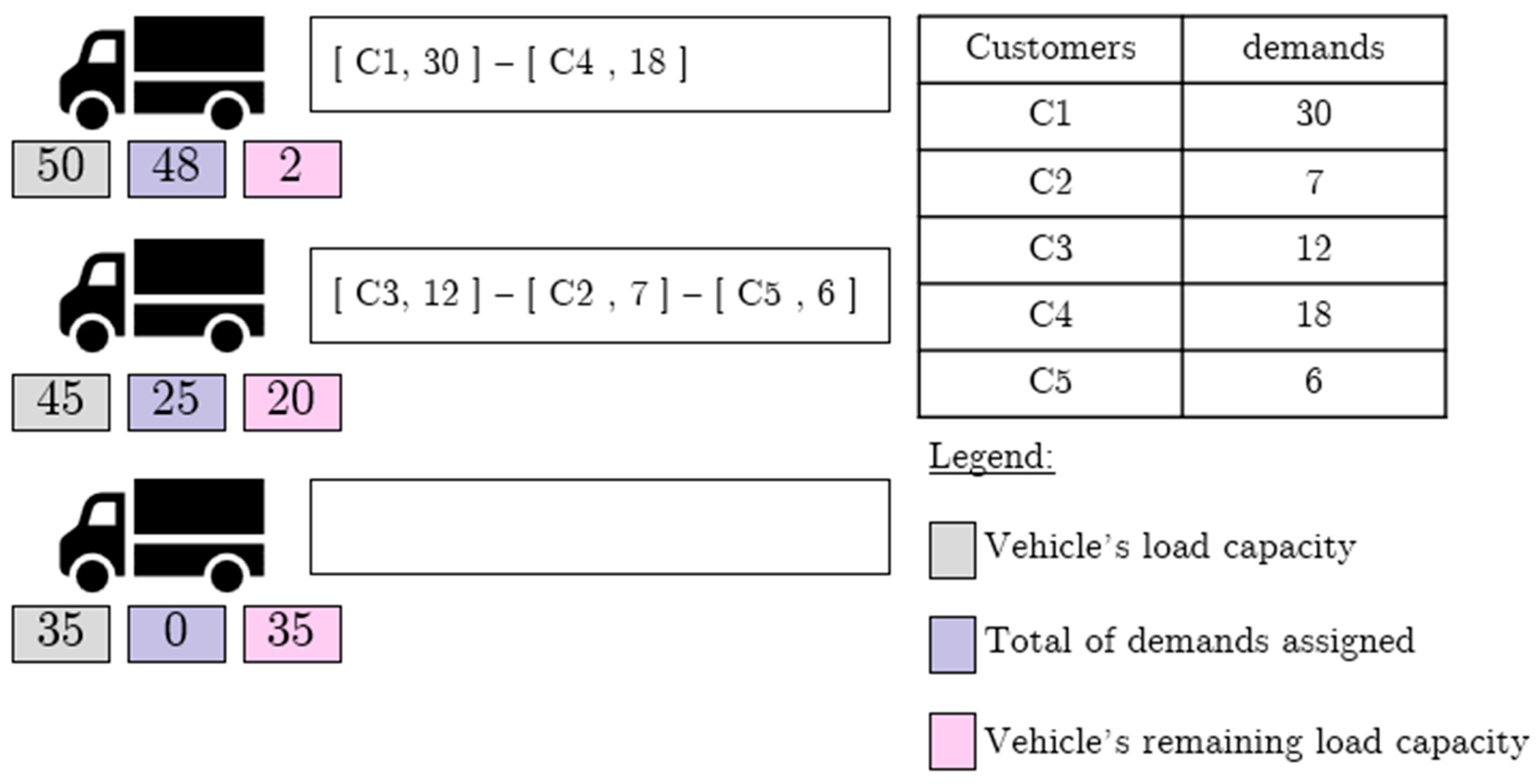
* The edge is the distance between two vertices. A vertex is either a station, a customer, or the warehouse.

explains the approach used to generate subtours. In an ideal scenario, a single vehicle will be able to serve all customers, but no vehicle is able to carry all customers’ demands at once unless it goes back and forth to the warehouse. Using one vehicle several times will almost certainly cause a delay in delivery and contradicts with the time windows available. This is easily proven when we consider the case of two customers with the same time window, where the time needed to drive from the first customer to the second, plus service time, surpasses the second customer’s time window. Our approach would not run into this issue, since we evaluate the fitness of each customer before assigning them to a vehicle.

We begin by selecting a vehicle from the fleet, which was already sorted by the remaining load capacity of the vehicles in descending order. Next, we find the customer with the biggest demand among the non-assigned customers. The selected customer cannot have a demand that surpasses the remaining load capacity of the current vehicle. We also do not want to assign a customer to different vehicles, as they would be visited more than once. If no customer can be served by the current vehicle, we move on to the next vehicle. Otherwise, we add the selected customer to the subtours list, along with the name of the vehicle to which they are assigned. We keep going until all customers are served. If, after assigning customers, a customer remains unassigned, we deem the dispatching unfeasible; thus, the whole delivery is impossible.

In Figure 3, we showcase an example of the vehicle dispatching approach where the fleet consists of three vehicles with different load capacities. We also have five customers with varying demands to serve. Using the previously explained approach, Algorithm 1. deploys two vehicles out of three, while respecting vehicles’ load capacities. Using this method, we are sure to avoid overusing the fleet we have at our disposal, thus respecting the fourth term of our approach, expressed by Equation (1).

4.2. Stage 2: Finding Optimal Paths Using the Genetic Algorithm

While other works used several approaches to solve the EVRP, such as ACO (Ant Colony Optimization) [21,22], variable neighborhood search [23] and artificial intelligence [24], in this paper, we resorted to GA. This algorithm was first proposed in 1975 by John H. Holland [25], in a time where the interest in heuristics was at its peak [26], and it mimics the evolution of living creatures.

GA follows a reproductive process in which the first population, named parents, pass down some of their characteristics to their offspring. Parents are the first set of paths generated randomly, from which we produce the next generations of paths. However, not all parents are allowed to reproduce. Using a fitness function that measures the strength of each parent, and setting a fitness threshold, only the parents whose fitness exceeds this threshold are selected.

Our paper applies the GA as previously undertaken in the literature, where an initial random population is generated, then coupled repeatedly to produce offspring. The algorithm starts by constructing a data matrix from the dataset provided. The data matrix gives the information displayed in Table 3.

The distance of an edge is a Euclidian distance, calculated using the coordinates of both ends of an edge (origin vertex and end vertex). We also consider that, if an edge from A to B exists, then an edge from B to A exists as well. As portrayed by Algorithm 2, the algorithm is also provided with information about the fleet of vehicles. For each vehicle, we need to specify its driving range, load capacity, weight, driver’s profile (experienced or beginner), battery capacity, and frontal area.

The overall procedure portrayed by Table 2 can be divided into the following three segments: optimal paths generation, charging stops selection, and stations assignments.

Algorithm 2. Genetic algorithm used to solve the capacitated EVRPTW (Electric Vehicle Routing Problem with Time Windows)

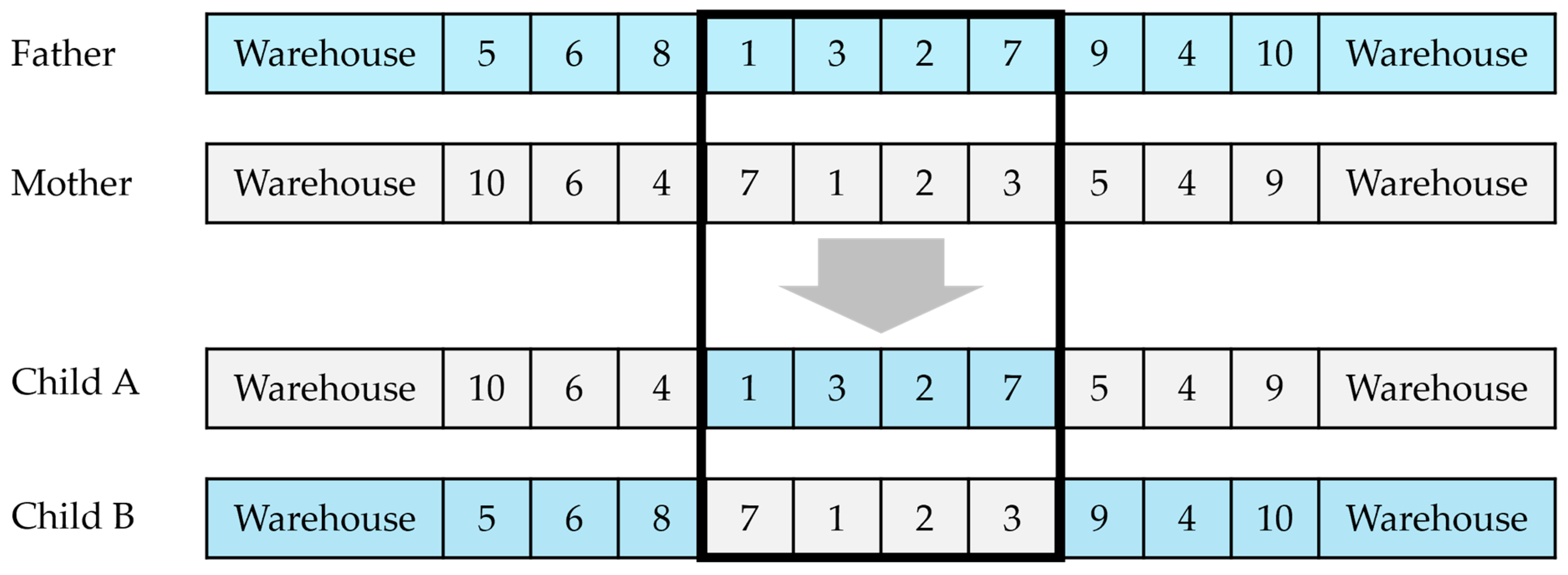
The crossover procedure was based on the 2-opt approach [27,28], in which two random points are selected within the length of the path. These two points mark the start and end of the crossover area, and all chromosomes (nodes) in this are passed down to the generated offspring as they are. Nodes on both sides of the crossover area are passed down to the offspring as well, but from another parent. The overall procedure of crossover is explained in Figure 4.

Table 3. Values of external parameters applied on the vehicles.

Parameter	Annotation	Value
Air density	$\rho$	1.2041 kgm−3 [29,30,31,32]
Air drag coefficient	$C_a$	0.48 [33]
Gravitational constant	g	9.81 m/s2
Rolling friction coefficient	$C_r$	0.013 [34]

Table 3. Values of external parameters applied on the vehicles.

Parameter	Annotation	Value
Air density	$\rho$	1.2041 kgm−3 [29,30,31,32]
Air drag coefficient	$C_a$	0.48 [33]
Gravitational constant	g	9.81 m/s2
Rolling friction coefficient	$C_r$	0.013 [34]

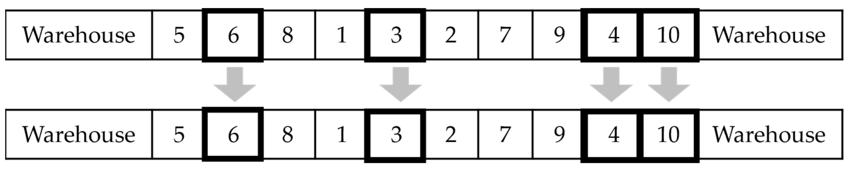
Mutation consists of choosing a random set of nodes in each parent and randomly redistributing them, as portrayed by Figure 5. Following crossover and mutation, any offspring that is deemed unfit is destroyed. A path is considered unfeasible if it visits the same node, or nodes, more than once, if it does not start or end at the warehouse, or if it has unconnected nodes.

To enhance the population diversity, random mutation points are selected for every path depending on its length. The first and last nodes are always excluded from mutation, as they represent the warehouse and are similar for all paths. A fit path can become unfit after charging station insertion, which we will discuss in stage 3.

Once the data matrix is constructed, customers are assigned to vehicles, using the previously mentioned approach via Table 2. Next, for each vehicle deployed, a set of randomly constructed paths, called parents, is generated from the already created subtours. Although these paths are random, they are verified using a fitness function to check their compliance to the requirements of our EVRP approach. The fitness function eliminates any path that has the following characteristics: (a) start and/or end vertices are different from the warehouse, (b) the path has unconnected vertices, or (c) repeated vertices. The surviving paths that are deemed fit proceed to the reproduction steps, as portrayed by

Table 4. Characteristics of the Volvo electric vehicles used for deliveries [35].

Vehicle	VOLVO FL	VOLVO FE	VOLVO FH
Number	7	7	6
Weight (in kg)	16,700	27,000	44,000
Power (in kW)	Up to 135	Up to 300	Up to 490
Battery capacity (Kwh)	200–395	280–375	180–540
Driving range (Km)	300	200	300
Frontal area (m × m)	2.282 × 2.723	2.500 × 2.849	2.500 × 3.394

.

Reproduction starts by selecting the most fit parents. This is carried out using a roulette selection method, in which the average fitness of all current parents is calculated, Parents with a fitness higher than the average fitness are selected while the rest are destroyed. Parents duplicates are also destroyed to avoid falling into a local optimum. Selected parents are then crossed two by two to produce new paths, called offspring. The fitness of every offspring is verified; thus, unfit offspring are destroyed. Surviving offspring are mutated two by two. To avoid premature convergence, and to create diversity among the population, mutation points are dynamic and vary from one pair to the other. Once again, any unfit offspring generated by the mutation process is destroyed. These steps are repeated until the iterations limit is met.

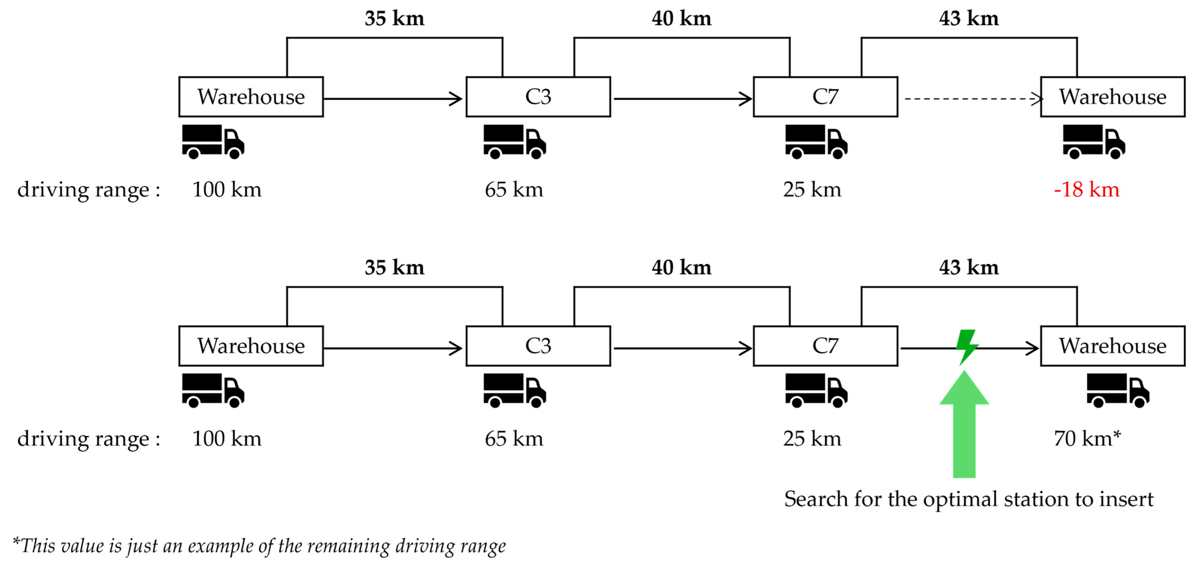
4.3. Stage 3: Charging Station Insertion

The paths that are generated in the previous segment of the approach are evaluated, and an optimal path for each vehicle is selected. The following step consists of finding the proper moment to recharge the vehicles, and the optimal station to stop at, as illustrated by Figure 6. The decision on when to recharge the vehicle is made according to the vehicle’s driving range. At every vertex $v_i$, the algorithm estimates the amount of energy needed to reach the next vertex in the path using Equation (16); the amount of energy consumed translates to a mileage that is deducted from the vehicle’s driving range. If the remaining driving range is negative, we set the previous vertex $v_{i-1}$ as a charging stop. This means that, once the previous vertex $v_{i-1}$ is reached, the vehicle must set out to the optimal station to recharge before travelling to vertex $v_i$.

The remaining driving range is the remaining mileage of the vehicle at vertex $v_i$, which depends on the station visited and its distance from both vertices $v_i$, and $v_{i-1}$. Since at this stage, we do not know which station to visit yet, we randomly pick the farthest station that is connected to both vertices (which is the worst-case scenario) and estimate the mileage remaining upon arriving at vertex $v_{i-1}$. From that point on, we repeat the same steps until we return to the warehouse.

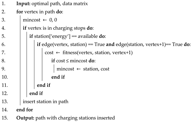
Upon arriving at this stage, the optimal paths for each vehicle and the charging stops are selected. Next, we need to decide on the station (or stations) to stop at every time we reach a charging stop.

As previously mentioned in Table 2, each station is designated a set of parameters, based on which we can make the decision whether to pick that station or not. These parameters are the distance to reach that station from another vertex, the waiting time (or queueing), and the availability of energy. The pseudocode is displayed by Algorithm 3, which explains the approach used to select stations.

Only stations with an existing edge with the vehicle’s current location are considered. The next crucial parameter to consider is the availability of energy. For all stations with available energy and an edge to the vehicle’s current location, we consider three factors: time, distance, and amount of energy acquired upon arriving at the station. The three factors are calculated for the path (actual vertex—station—next vertex).

Algorithm 3. Stations assignment approach

Our approach, expressed by Equation (1), prioritizes time minimization, which means that, when selecting a station, we select the station that generates the least time to reach the next customer. This time includes the travel time from the actual customer to station, the waiting time once at the station, the time needed to acquire energy, which depends on how much energy the vehicle has upon arriving to the station, and the travel time from station to next customer. If two stations have the same travel time, we pick the station with the least travel distance. If two stations have the same travel distance, we compare the amount of energy consumed throughout the path and pick the station resulting in the least amount of energy consumption. Similar to the time of travel, both distance and energy are calculated along two arcs: actual customer to station and station to next customer. In cases of two or more stations having equal costs, a station is selected randomly.

We assume that once a station is picked, the queuing time is fixed and does not go up. This means that the vehicle reserves a place at the station before making its way to it. It also means that the travel time from the actual vertex to the station is deducted from the waiting time.

5. Simulation

The algorithm for our approach was run using Google Colab Pro Plus, using 32 GB of RAM, and A T4 GPU. Simulations were run on 36 instances with different sizes and layouts, organized as follows:

• 12 sets of instances, each with 5 customers;
• 12 sets of instances, each with 10 customers;
• 12 sets of instances, each with 15 customers.

Each set of 12 sets of datasets was split into three categories of four instances, according to the nodes’ (customers’) layout: clustered, random, and a combination of both. The term ‘layout’ describes the way customers are dispersed geographically.

Each set was run for 1000 generations. Generations were repeated 10 times each.

Aside from the dataset and the fleet deployed, the overall driving experience was subject to several external factors, such as air density and rolling friction gradient, as expressed by Equation (16). Table 3 summarizes the values used for simulation.

5.1. Dataset

To evaluate the strength of our approach, we chose to run simulations on Schneider’s instances [36], which are based on Solomon’s benchmark instances [37]. Although these instances were introduced in 2014, several works were conducted using them throughout the years, such as the work in [23], in which a multi-depot scenario was considered. Another recent work that used nearly the same scenario as our approach on the previously mentioned instances is a work in [38]. In another setting, the work in [39] considered capacitated charging stations to solve the EVRPTW, using a branch-and-cut-and-price approach. A similar approach was used in [40,41]. In a recent work, [42], a combination of adaptive large neighborhood search method and greedy heuristic was performed using Schneider’s instances. The choice of this dataset provides us with a reference to compare our approach to, which will help shed light on its strengths and weaknesses.

In the dataset used, we had access to the following information: vertex coordinates, demand, time window, and service time. This dataset provided several instances of three different layouts: clustered vertices, randomly scattered vertices, and a combination of both.

5.2. Fleet Characteristics

The fleet deployed was supposed to be heterogenous. In our approach, we chose an altered version of Volvo Electric Trucks [35], which come in five different versions. For cost reasons, we picked only three approaches, whose specifications are portrayed in

Table 5. Examples of optimal solutions to 5-, 10-, and 15-customer instances.

Dataset		Path	Time (min)	Distance (km)	Energy (KJoules)	Exe. Time (s)
Size	Reference
5	C208C5	WH-C50-C53-C58-C60-C39-WH	599	156	419	236
	R104C5	WH-C87-C71-C99-C1-C5-WH	99	213	112	231
	RC208C5	WH-C66-C96-C32-C37-C41-WH	89	170	101	269
10	C101C10	WH-C13-C100-C54-C78-C96-C95-C98-WH	954	283	917	1151
		WH-C4-C89-C27-WH	211	106	108
	R201C10	WH-C100-C18-C50-C31-C84-C94-C72-C28-C32-C77-WH	185	259	261	1063
	RC201C10	WH-C93-C22-C88-C98-C54-C14-C79-C81-C62-C43-S15-WH	330	426	610	1030
15	C208C15	WH -> C7 -> C85 -> C82 -> C31 -> C88 -> C75 -> C22 -> WH	968.4	257	1.80	8105.92
		WH -> C79 -> C98 -> C73 -> S19 -> C59 -> C43 -> C52 -> WH	870	272	918.39
		WH -> C24 -> C20 -> WH	107.4	30	0.19

Charging station are marked in bold.

. The choice of vehicles was made arbitrarily, as the five versions had enough load capacity and driving range and, thus, could be used in our approach.

The fleet size was the same for all sizes of instances, because our dispatching method ensures that only the needed number of vehicles will be deployed. The approach was designed in a way that prioritizes the selection of the vehicle with the largest load capacity first, which was set between 150 kg and 300 kg. While the vehicles used for simulations had a larger load capacity of up to 38 tons, for simulation purposes, we reduced the load capacity of these vehicles, since the demands of customers in our dataset does not exceed 100.

5.3. Infrastructure Data

In the dataset used, we had access to the following information: vertex coordinates, demand, time window, and service time. However, we still needed more information, such as temperature, slope, speed limit, traffic status, and waiting times. In the absence of an API (Application Programming Interface) to communicate this information with vehicles, we resorted to a randomly generated set of data that could be frequently updated, if needed, to mimic real-life ever-changing settings. For every dataset, the infrastructure data were generated once before the first iteration and were maintained the same throughout the following iterations.

Table 6. Infrastructure data generated for nodes of the RC201C10 dataset.

Edge	Distance (km)	Speed (km/h)	Slope (°)	Speed Limit (km/h)	HVAC Driver	HVAC Trunk	Traffic (%)
WH-S3	36	90	27.44	50	ON	ON	29
C98-C14	22	110	14.78	50	ON	ON	84
S3-C98	43	90	17.93	60	ON	ON	21
S9-C14	16	90	24.88	70	OFF	OFF	72
S9-C79	12	10	4.27	60	OFF	ON	83
S15-S9	41	20	14.01	60	OFF	OFF	50
S9-C79	12	10	4.27	60	OFF	ON	83
C98-WH	14	90	26.67	120	ON	OFF	5
C98-C54	30	80	18.3	50	ON	OFF	5
C14-C43	64	60	3.93	20	ON	ON	87
C81-C93	13	90	2.41	50	OFF	ON	21
C62-C14	60	50	15.87	40	ON	OFF	68
C43-S9	48	90	32.62	40	ON	ON	3
C22-C81	43	50	33.14	40	ON	ON	31
C54-C93	10	50	13.31	50	OFF	OFF	24
C79-C22	62	10	30.56	30	ON	OFF	21

illustrates an example of infrastructure data generated for RC201C10 dataset, where WH stands for warehouse. Station S0 was not considered, since it exists in the warehouse itself. Regarding road condition, we generated information related to traffic, speed of the vehicle, speed limitation, road slope, and temperature. We ignored the case of blocked roads and considered all edges to be available, as heavy as traffic might become.

While data were generated randomly, they still abided by a few rules, as follows:

• Temperature was limited to [−5 °C, 12 °C] in winter and [12 °C, 40 °C] in summer. The temperature depended on the season, which was defined in advance, and the season was the same for all vertices.
• The road slope was, at most, 37° as that is the steepest slope in a residential area in the world [43].
• Parking time was, at most, 15 min.
• Speed was, at most, 120 km/h but could be less, depending on the traffic and the speed limit.
• The speed limit varied from 20 km/h to 120 km/h.
• Traffic was expressed using a percentage between 0% and 90%. For instance, if traffic was 10%, and the speed along the arc was 80 km/h, the final speed was 72 km/h, which is 10% less than 80 km/h.
• The use of auxiliaries and HVAC depended on the season, as well as the time of day. For instance, if the season as set as summer, the use of windshield wipers was set as OFF. Otherwise, it varied, depending on whether it was raining or not. The information about rainfall was generated randomly and could change from one edge to another.

To be able to compute the time of travel across an edge, the speed needs to be known. To this end, the data update process also generated speed across all edges. This speed was affected by the driver’s style of driving, mainly regarding the amount of acceleration applied; for aggressive drivers, acceleration was 3 to 4 m/s², while it was 1.5 to 2 m/s² for experienced drivers [8,44].

The driver profile was linked to the vehicle, which meant that once a vehicle was selected, the amount of acceleration assigned to it was applied on all arcs driven by this vehicle.

6. Results and Discussion

To keep results consistent, road conditions were generated once for each type of set and preserved the same for all remaining iterations. Since all nodes were connected, and at the risk of being too extensive, only a portion of data is shown. We have established that all edges are supposed to be symmetrical; this means that the infrastructure data from vertex i to vertex j are identical to the infrastructure data from vertex j to vertex i.

Due to the complexity of the approach, the first population was set at 10 for all datasets of 5 and 10, while it was set at 15 for instances of 15 customers, to reduce computational time. Larger first population sizes increased the computational time remarkably, without enhancing the final solution.

As time is the first component of our approach, expressed by Equation (1), solutions with the lowest travel time were considered optimal. If two paths had equal travel time, we selected the optimal path based on the travel distance. Finally, energy consumption was the last selection criterion.

For multi-vehicle solutions, the same rules applied regarding the total time, total distance, and total energy consumed. However, if a solution had a component that was considered the worst amongst all solutions, the solution was discarded and the next best solution was selected.

According to the selection criteria mentioned previously, one solution was selected for each dataset. Table 5 portrays the 12 optimal solutions for instances of 5 to 15 customers, wherein WH refers to the warehouse, C refers to customers, and S refers to stations.

For five-customer instances, due to the choice of vehicles, neither solution required more than one vehicle, nor a stop at a charging station. For 10-customer instances, the vehicles did not need to stop at a charging station in the case of randomly scattered customers. Furthermore, the approach mainly used one vehicle for all instances, except for clustered instances of 10 customers, where two vehicles were deployed every time. Furthermore, we noticed that the solutions for randomly scattered customers—for both sizes of instances—required less time, distance, and energy consumption, and that our approach solved them faster than clustered or clustered–random customers instances.

The generated solutions also showed that clustered customers generally required higher costs to serve. As stated by the objective function, expressed by Equation (1), cost is time, distance, energy, and number of vehicles deployed.

While time and distance are proportional, the increase in the travel time is not necessarily caused by an increase in the distance. Table 5 shows that mostly, consumed energy increased with travel time, while distance was only impacted by the path selected. Since our version of the EVRP incorporated infrastructure in the mathematical approach, traffic, for instance, increased travel time and impacted energy consumption as well, without adding to the driven distance. This conflict explains why some of the worst solutions had smaller travel distances, when compared to optimal solutions. This means that the algorithm often selected a path with a longer distance to reduce travel time and avoid traffic-blocked edges, edges with speed restrictions, roads with steeper slops, or farther stations, where the waiting time added to the time taken to reach them is less than closer stations, where the waiting time is higher.

While execution time for our approach is rather greater than other conventional methods, this can be easily justified by the fact that our approach is weighted down by several constraints, such as energy consumption that is calculated for each arc and infrastructure that not only increases travel time but also increases the chance of paths’ unfeasibility, forcing the algorithm to hunt for another potential solution. Furthermore, once a solution is selected, the algorithm moves on to the second step, which is station insertion. At this point, it is relatively possible that the path becomes unfit, which requires looking for the second-best solution among the surviving population and repeating station insertion again.

From a certain point of view, avoiding charging stops appeared to decrease the overall travel time and helped make the most of the vehicle’s driving range. However, when traffic was added to the equation, a path with a charging station could be less time-consuming, given that the arcs used had less traffic, and the station had little to no queue. The solution for dataset ‘C205C10’ confirms this theory.

The first thing we can highlight regarding the solutions to 15-customer datasets is the higher amount of energy consumed throughout these paths, which is linked directly to several factors, as previously mentioned in Equation (16). It should be noted that these values of energy are logical, seeing as we subjected the vehicle to extreme varying conditions. The objective, aside from finding the optimal path, which our approach was already capable of, and generating the least costs possible, was to challenge the approach in extreme dynamic situations.

Although real-life settings are dynamic and unforeseeable, they still are not as extreme as those randomly generated in our approach. For instance, traffic is usually heavier in certain intervals of the day and in specific regions. However, in our approach, traffic was heavier than normal at most edges, regardless of the time of the day. In addition to traffic, we added speed limits to challenge the approach even more. This helped to ensure that the approach can be functional and reliable in almost any situation.

Similar to 5- and 10-customer datasets, the approach used only the number of vehicles needed to carry on delivery operations in an optimal way and assigned the optimal stations to visit when needed.

Another important detail to mention is the impact of customers’ layout on the number of vehicles used. When customers were gathered in a certain region, the algorithm seemed to deploy more vehicles to serve them, compared to when customers were randomly dispersed. In some cases, the approach needed one vehicle only to serve the 15 customers, which was the case for the ‘R202C15’ dataset. In contrast, all clustered customers datasets required three vehicles to serve all customers.

Since the approach prioritizes time minimization over distance, it usually tended to avoid short routes where traffic, for instance, was heavy, or when infrastructure restrictions, such as speed limitations, were strict. Figure 7 illustrates the selected solution for dataset RC201C10, where it is noticeable how the approach avoided some edges, such as Customer 98 to Customer 14. According to the infrastructure data portrayed by Table 6, the path from Customer 98 to Customer 14 was almost blocked by a traffic congestion of 84%, which translates directly to a decrease in the velocity of the vehicle. To avoid slowing down, the approach resorted to going directly from customer 98 to customer 54, although the distance connecting these two customers surpassed the distance between customer 98 and customer 14, where traffic was a mere 5%. This phenomenon applied to all solutions; the approach made its decision based on the time it took to go from one node to another and chose the solution with the minimal time.

(a)

Comparison between optimal and worst solutions

As previously noted, we noticed that randomly distributed customers required fewer vehicles to serve them, compared to clustered customers. Furthermore, regardless of road conditions, random customers datasets generated less cost and had more consistent solutions. In other words, the gap between optimal and worst solutions was negligeable when customers were randomly distributed. This assumption is true and unrelated to the size of the dataset.

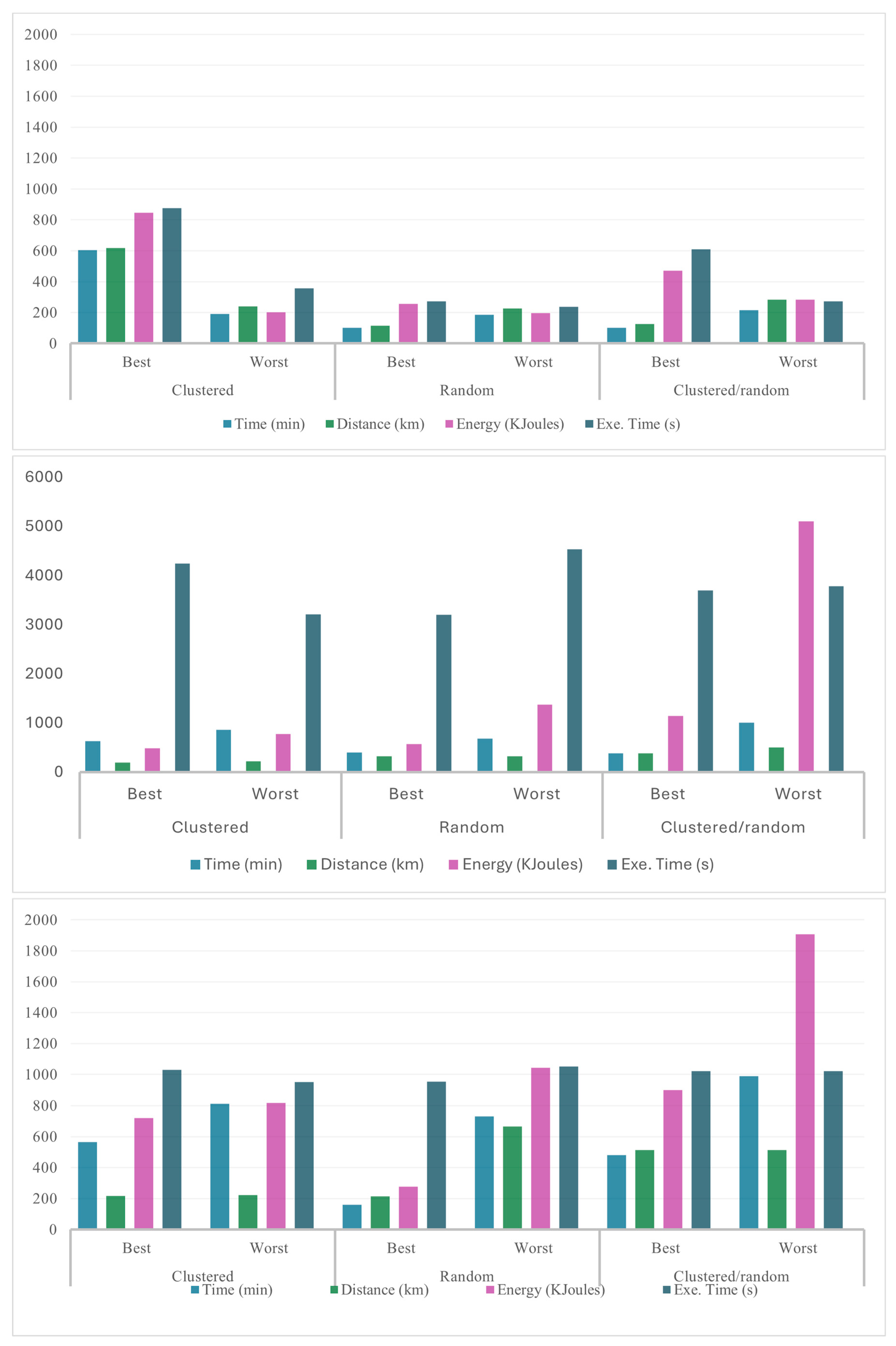
When it comes to 15-customer datasets, the results seemed to be, to some extent, even. Figure 8 illustrates the gap between optimal and worst solutions for medium sized datasets. We can notice how values were similar, unrelated to the customer distribution, except for energy consumption when customers were both clustered and randomly distributed.

When customers were clustered, the algorithm became somehow trapped in a certain region and was forced to use certain edges to serve customers, which led to an increase in total costs. However, when customers are far apart, although this might have added to travel distance, the algorithm had more room to navigate the edges connecting these customers.

(b)

Impact of number of customers and their distribution

In the case of 15 customers, the approach, as expected, took more time to complete the 1000 generations, compared to smaller instances, which is portrayed in

Table 7. Average computation time required for each dataset size and layout.

	Average Computation Time
Number of Customers	Clustered	Random	Random/Clustered	Overall
5	363.35	243.52	283.09	296.66
10	984.365	947.03	1026.86	986.08
15	4100.48	4166.66	3602.79	3956.64

. This increase was proportional to the number of customers. The more customers to serve, the more edges to choose from, and consequently, the more infrastructure data to abide by.

The time required to find the optimal solution for 15-customer datasets was almost 14 times the time needed for 5-customer datasets. Moreover, customers’ layout did not appear to have a considerable bearing on computation time, since the average computation time for different layouts were close. Aside from the EVRP being classified as an NP (Nondeterministic Polynomial time) hard problem, including multiple constraints to the approach weighed down on its computation speed, which is the reason why we withdrew from running simulations on 100-customer datasets. When trying to solve 50-customer datasets or higher, the algorithm would run for more than 12 h. This does not, by any means, imply that our approach is incapable of solving large-sized instances, but it just requires more time than we have on our hands for the moment.

7. Conclusions and Future Works

In this paper, we tried to tackle the electric vehicle routing problem, also known as the EVRP, with time windows in extreme settings and using a heterogenous fleet of vehicles. Following on from the classic EVRP goal, our approach aimed to serve a set of customers at the optimal costs possible. Our approach, expressed by Equation (1), focused on the minimization of four interrelated components: time, distance, energy, and the number of vehicles.

One of the main weaknesses of the EVRP is its inability to replicate real-life settings, which often renders the proposed approaches unpredictable when facing real-life settings (traffic, for instance). To this end, we included factors like speed limit, temperature, driver profile, road slope, vehicle’s speed, weather conditions, time of day, and auxiliaries usage to our approach. In an ideal scenario, the vehicles would be able to receive all infrastructure data in real time, giving the approach the opportunity to adapt its search approach accordingly. However, in the absence of an API to communicate with the vehicles, we generated a random set of infrastructure data, which was used afterwards as an input for the algorithm.

To solve our version of the EVRP, we proposed an enhanced version of the genetic algorithm, where the dispatching of vehicles was conducted before the search for an optimal solution. Our solution started by assigning customers to vehicles, then treated each set of customers assigned to a certain vehicle as a single case of the TSP (travelling salesperson problem). Once the solution was found, the algorithm inserted the optimal charging station at the optimal moment, when, and if, needed.

Upon running simulations on 5- to 15-customer-sized datasets, we noted that our approach was successfully able to converge towards an optimal solution within a reasonable computational time, while navigating a web of heavily constrained edges. The approach successfully added charging stations to the selected paths, while complying with the collection of required constraints. However, due to the heavy load of constraints considered, we refrained from solving larger dataset instances, due to the long computational time needed. This long computation time was due to the extreme conditions under which we put our approach, and the excessive number of constraints that it needed to respect.

In future works, we aim to expand our efforts to solve larger dataset instances in reasonable time while mimicking real-life dynamic settings. We also aspire to reduce the actual execution time for 5- to 15-customer-sized datasets.