


A Risk Assessment Framework for Cyber-Physical Security in Distribution Grids with Grid-Edge DERs

Department of Electrical and Computer Engineering, University of Central Florida, Orlando, FL 32816, USA
*
Author to whom correspondence should be addressed.
Energies 2024, 17(7), 1587; https://doi.org/10.3390/en17071587
Submission received: 1 March 2024
/
Revised: 16 March 2024
/
Accepted: 19 March 2024
/
Published: 26 March 2024
(This article belongs to the Special Issue Smart Grids and Microgrids: From Simulations to Experimentation)
Abstract
:Integration of inverter-based distributed energy resources (DERs) is reshaping the landscape of distribution grids to fulfill the socioeconomic, environmental, and sustainability goals. Addressing the technological challenges of DER grid integration requires an adaptive communication layer for efficient DER management and control. This transition has given rise to a cyberphysical system (CPS) architecture within the distribution system, causing new vulnerabilities for cyberphysical attacks. To better address potential threats, this paper presents a comprehensive risk assessment framework for cyberphysical security in distribution grids with grid-edge DERs. The framework incorporates a detailed CPS model accounting for dynamic DER characteristics within the distribution grid. It identifies vulnerabilities in DER communication systems, models attack scenarios, and addresses communication latency crucial for inverter control timescales. Subsequently, the quantification of attack impacts employs an attack probability model including both the vulnerability and criticality of cyber components. The proposed risk assessment framework was validated through testing on the modified IEEE 13-node and 123-node test feeders.
1. Introduction
The traditional distribution grid is shifting from a unidirectional electricity flow model to an active distribution grid with bidirectional electricity flow capabilities. This transition is driven by the imperative to address environmental, socioeconomic, and sustainability goals, resulting in a distribution grid with high penetration of the distributed energy resources (DERs) at the edge. These DERs facilitate the incorporation of diverse renewable energy sources into the primary grid through interfaces like synchronous generators, induction generators, and inverter-based resources. Notably, inverter-based DERs have gained considerable traction due to specific attributes, including improved power quality by minimizing harmonics, control of reactive power and voltage across a wide power factor range, and rapid responses for tasks like high-frequency regulation, quick switching, and fault isolation.
Inverter-based DERs present challenges despite their advantages [1]. The first challenge involves system reliability, primarily stemming from the inherent uncertainty in renewable energy sources. Despite employing multiple forecasting methods to estimate inverter output, accurately predicting the variance between forecasted and actual values remains elusive. In networks with high penetration of DERs, this cumulative forecasting error can lead to significant reliability issues, particularly when reserve capacity is insufficient [2]. The second challenge pertains to system stability. Inverter-based DERs have low inertia [3], which can diminish the system stability margin. Consequently, disturbances that are typically manageable in traditional synchronous machine-dominated grids, such as load switches, system reconfiguration, and short-term faults, may provoke stability concerns in DER-dominated grids. This will sometimes result in large-scale blackouts. The third challenge revolves around system protection. Existing protection devices are primarily designed to respond to high-amplitude fault currents, a characteristic common in synchronized machines. However, fault currents in inverters are typically of smaller magnitude, potentially failing to activate protection devices promptly [4]. Consequently, faults in inverters may not be promptly isolated, leading to voltage or frequency violations and potentially triggering cascade failures.
To overcome these challenges, an efficient communication network is essential for real-time monitoring and control of DERs. This network enables bidirectional data exchange, handles increased sensors and actuators, adapts to the complex topology of dispersed DERs, and allows third-party involvement for collaborative efforts among stakeholders, such as DER owners, manufacturers, and aggregators [5].
Distribution grids incorporating a communication network for DER management and control manifest a cyberphysical system (CPS), which has significantly expanded the potential cyberattack surfaces [6,7,8]. Slower safety mechanisms and protection devices behind the expanded cyber networks have made vulnerabilities easier to exploit. Moreover, the requirement to involve DER manufacturers, owners, and third parties can lead to incomplete or underdeveloped authorization and access protocols, posing a substantial risk to distribution network stability and reliability. Therefore, an extensive risk assessment framework becomes crucial for ensuring the cyberphysical security of distribution grids with grid-edge DERs.
A detailed CPS model embedded with the interdependency of cyber and physical elements is crucial for risk assessment, ensuring precise evaluation of the potential attacks’ impact [9]. Simultaneously, calculating the likelihood of these attacks is equally important. Given the defense resources constraints, identifying the most frequent attacks becomes imperative. An accurate attack probability model guarantees the optimal selection of defensive strategies, thereby fortifying CPS resilience.
Several CPS risk assessment methods have been proposed. Some of them deploy conventional probability evaluation methods. For instance, [10] introduced a cyber risk strategy focused on protection systems. This approach uses Monte Carlo methods to simulate compromised protection components, identifying cascade failures and load-shedding effects. Ref. [11] introduced an attack graph-based method to evaluate the cyber risk of the cyberphysical power system. In [12], authors used the stochastic game theory to model attacker and defender behaviors in order to assess cybersecurity risks. The works from [13,14] employed the Bayesian network to address CPS cyberphysical risks related to system vulnerabilities. Additionally, emerging learning-based methodologies have gained popularity in recent years. These methods, compared to conventional approaches, are more suited for large-scale system analysis. For instance, [15] utilized deep reinforcement learning to find optimal network transition policies from the attacker’s perspective, evaluating potential attack impacts. Ref. [16] presented a rank algorithm based on learning methods to achieve real-time risk evaluation. However, they typically necessitate large amounts of data for the training set, which can be challenging to collect in real-world scenarios, posing feasibility issues.
Nevertheless, these works in the literature are generally based on the steady-state model, which typically treats DER behavior as PV or PQ buses and overlooks crucial DER functionalities outlined in the IEEE 1547-2018 standard [17], such as Volt-Var support and ride-through capabilities. Consequently, these works fail to capture the dynamic behavior of DERs, potentially leading to inaccurate results. Therefore, a comprehensive cyberphysical system (CPS) model incorporating dynamic DER behavior is essential for accurately assessing the potential impact of cyberattacks on DERs.
Moreover, current frameworks often oversimplify the communication layer by employing time-static models or treating potential cyberattacks merely as contingencies, assessing their impacts through contingency analysis. However, with the integration of inverter-based DERs, communication latency can significantly reduce the system stability region, especially in scenarios with high DER penetration [18,19]. This emphasizes the need to consider communication system latency for precise cyber risk assessment within such systems.
Furthermore, within the impact quantification, it is crucial to link the attack probability to both the “cost” (vulnerability) and “reward” (criticality) of a component. Previous studies have often focused on one of these aspects or assumed a fixed probability distribution for attack likelihood, which might not accurately reflect current attack patterns.
To address the aforementioned limitations, this work introduces a novel cyber risk assessment framework for active distribution grids with inverter-based DERs. The innovative steps within the proposed framework are as follows:
- A DER-explicit distribution grid model accounting for dynamic attributes of inverter-based DERs.
- A high-fidelity DER communication layer model with communication latency to facilitate the precise execution of cyber layer attacks.
- A cyberattack risk quantification method based on an attack probability model that accounts for both cyber component vulnerability and criticality.
The paper structure is as follows: Section 2 outlines the proposed risk assessment framework. Section 3 describes the DER-explicit CPS model. Section 4 delineates cybersystem vulnerabilities and cyberattack models. Section 5 introduces the method for risk quantification. Simulation results and conclusions are discussed in Section 6 and Section 7.
2. Proposed Risk Assessment Framework
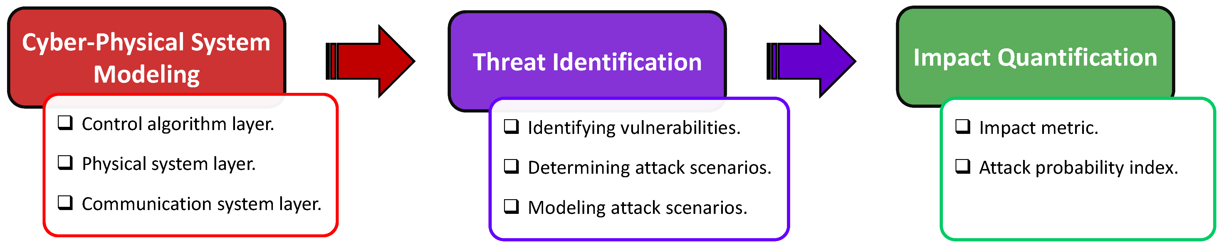
The proposed risk assessment framework comprises three main sections, as shown in Figure 1: (i) cyberphysical system modeling, (ii) threat identification with cyberattack models, and (iii) impact quantification. This framework enables rapid snapshot analysis, focusing on steady-state evaluation. Moreover, due to the integration of the inverter dynamic model, it also facilitates accurate simulation of dynamic behavior, allowing for a detailed exploration of the potential impact of cyberattacks on the physical system. This framework has a modular structure, offering scalability and flexibility to incorporate other modules. Once the system configuration is collected, this framework can be tailored accordingly. It enables the assessment of risks posed by specific attacks and identifies the most vulnerable components in the cyber layer. Consequently, it provides valuable insights for crafting effective defense policies.
2.1. Cyberphysical System Modeling
The first and foremost important section is the CPS model of a distribution grid with inverter-based DERs. The proposed cyberphysical distribution system (CPDS) includes three layers: (i) the control layer, (ii) the physical system layer that embodies a DER-explicit distribution grid, and (iii) a communication layer manifesting interaction among the control and physical layers.
The optimal power flow (OPF) and load-sharing control represent examples of control algorithms tailored to achieve specific control objectives in physical system operation. It is important to recognize that various other DER control algorithms can also be deployed within this framework. However, different algorithms operate on distinct time scales and may necessitate different data exchange patterns. Given the low inertia of inverter-based distributed energy resources (DERs), these nuances are critical for accurately assessing risk, underscoring the necessity of specifying them prior to conducting risk assessment.
A DER-explicit unbalanced distribution system constitutes the physical layer of CPDS. With a focus on a distribution grid characterized by high DER penetration, the power-flow (PF) equations for the unbalanced distribution grid are utilized for steady-state analysis, complemented by the virtual oscillator controller (VOC)-based dynamic inverter model for dynamic analysis.
Finally, the communication layer within the CPDS employs a graph-based mapping function that captures the data exchange patterns between the control and physical system layers. This model also integrates time-stamp data for dynamic modeling and introduces communication system latency, which is essential for accurately representing the system’s dynamic characteristics.
2.2. Threat Identification
This section identifies potential threats to the DER communication network and assesses their probable impacts. In this section, the first step is to collect the cyber layer configuration, such as gateway info (manufacturer, software version) communication protocols, and so on. Based on the given information, the system vulnerability can be identified according to the vulnerability database. In this framework, the National Vulnerability Database (NVD) is utilized for vulnerability identification. Given the variety of threats, some could pose a risk to data confidentiality, potentially resulting in financial losses for utilities or customers, and others have the capacity to disrupt grid operations significantly, giving rise to concerns about public safety. This work primarily focuses on the latter category of attacks. To analyze the impact of cyberattacks, a suitable attack model is developed that aligns with the CPDS cyber model. This model can be integrated into the previously proposed cyberphysical interdependency model, capturing the atypical cyber component behaviors when attackers exploit vulnerabilities, leading to the execution of an attack. Through simulation of the CPDS model, the propagation of such attacks can be identified, thereby enabling determination of their potential impact on the physical layer.
2.3. Impact Quantification
To quantify impact, let i denote the cyber component index. The risk for the ith cyber component being attacked is defined as follows:
Here, represents the degree of impact, specifically the financial repercussions in this work, which is caused by the ith component being compromised. This assessment is facilitated by integrating the attack model with the proposed CPDS model, as discussed earlier. The parameter denotes the attack probability index, indicating the likelihood of the ith node being targeted. This is grounded in a cost–reward decision-making model. The associated “cost” reflects the “difficulty” of compromising a cyber node, established based on a Bayesian network using vulnerabilities identified in the preceding section. The “reward” is determined by the criticality of components, modeled as sensitivity in this study, i.e., the extent of change in physical state variables when the cyber variable transmitted in the component deviates from its desired value. This sensitivity is derived from analyzing the cyberphysical model for a given attack type. The overall attack probability index is calculated using the expected utility function, which amalgamates the “cost” and “reward” from the attackers’ perspective.
In the subsequent sections, each topic will be introduced in detail.
3. Cyberphysical System Modeling
Figure 2 provides an overview of the CPS model. The proposed model comprises three layers: (i) the control layer, (ii) the physical system layer representing a DER-explicit distribution grid, and (iii) a communication layer illustrating the interaction between the control and physical layers. These layers are depicted as time-dependent functional modules. These modules interconnect through a closed-loop data flow, where data serve as inputs and outputs for each module. Initially based on the static cyberphysical model proposed in [20], we adapted it into a time-variant model to suit our low-inertia inverter-dominant CPS. Let t denote time and represent the measurement data collected at time t, encompassing voltage, power information, etc., thus serving as the output of the physical system layer at time t. Similarly, denotes the control command reflecting the output of the control layer at time t, encompassing operational commands generated for the inverter, such as real and reactive setpoints. The communication system layer further divides into two submodules: the measurement data path module and the control command path module . These modules delineate the data flow pattern and time latency. Consequently, for the module, the output is denoted as , which becomes the input of the control layer. Similarly, refers to the output of module. At the same time, it also refers to the input of the physical layer. Thus, by properly modeling the attacks, their propagation pattern and the potential impact can be derived from this CPS model. More details about each layer are elaborated in subsequent sections.
3.1. Control Layer
In this work, two control algorithms will be analyzed based on the desired control objective for the physical system operation.
3.1.1. Algorithm 1
The first control algorithm is the optimal power flow (OPF) [21], with updates every 15 to 30 min. The objective of this algorithm is to regulate DER output, thus minimizing transmission-side power consumption costs and minimizing voltage deviations. Within this control, the control command carries the information of active and reactive power setpoints and is dispatched to each DER through the communication network. Let us consider a three-phase unbalanced distribution grid with buses and lines, and a set of inverter-based DERs. The OPF problem can be formulated as follows:
In (2), and are weight coefficients, refers to the complex voltage phasor of each bus, and indicate the real and reactive power of each line. The equality equations set refers to the power flow equation, where and denote real and reactive power from the substation and DER, respectively. The indicates the nominal voltage value. Additionally, the superscripts “min” and “max” correspond to the lower and upper limits of the respective variables and parameters.
3.1.2. Algorithm 2
In the second algorithm, the scenario assumes that the distribution-level OPF algorithm is unavailable. Consequently, we treat the distribution grid as a single bus and execute the OPF algorithm at the upstream or transmission control center. Control variables are defined as real and reactive power at the point of common coupling (PCC) on the distribution side. DERs are capable of load sharing [22] and regulating real and reactive power at the substation level by exchanging output real and reactive power information with neighboring units. At steady state, the real and reactive power at the PCC achieves desired values, while the power ratio of each DER remains constant, as expressed in the following equation:
3.2. Physical System Layer
A general mathematical model for an unbalanced distribution grid with inverter-based DERs is presented here.
3.2.1. System Dynamic Model
The dynamic model of three-phase unbalanced distribution with inverter-based DERs can be described by a set of differential-algebraic equations (DAEs) [23]:
Here, denotes a set of differential equations representing the dynamics of inverted-based DER generators, and represents PF equations. The vectors and denote dynamic state variables (e.g., system frequency) and physical algebraic variables (e.g., voltage magnitudes and phase angles), respectively. Finally, represents a vector of physical control variables (e.g., droop coefficients), and is a vector of system parameters, e.g., nodal injections including setpoints, i.e., .
The DERs are modeled as virtual oscillator controller (VOC)–based inverters, with multiple advantages compared to other control algorithms, such as droop or VSM [21]. The control framework is based on [24]. By leveraging a phase-decouple technology, this framework is able to be employed in a highly unbalanced network. Figure 3 illustrates the hierarchical inverter control framework (using phase a as an example). The inverter is first operated in the synchronization mode. When the voltage and phase differences between the grid and inverter are small enough, the inverter can be connected to the grid and start working in GFL mode, where are the active and reactive power set points from the control layer. When operating in the load-sharing mode, are replaced by the neighbor’s power ratio.
The VOC dynamics can be represented as follows:
where is the averaged terminal-voltage magnitude, and denotes the averaged phase offset. and are the averaged active and reactive output power of the inverter, respectively. and are preselected design parameters. The regulation of the inverter is achieved by continuously tuning two parameters, the voltage scaling factor and the virtual capacitor c, based on the control objective from the secondary control layer.
3.2.2. Steady-State Model
Consider the three-phase unbalanced distribution grid introduced previously in the section. A general expression for the ith bus complex voltages can be written as a function of nodal power injections and complex voltage phasors of all buses in the network as follows:
where is a dense matrix with complex entries. The structure of is defined through grid topology and line parameters [25,26]. The (6) refers to the algebraic equation set depicting load flows in the unbalanced distribution grid.
For the steady-state analysis, the power system model in (4) operates around its equilibrium, which is defined by the solutions of the algebraic set by equating the derivatives of dynamic state variables to zeros. Under normal operation, the slack bus (substation) is treated as an infinite bus. However, because of the potential cyberattacks, the power extracted from the substation may severely exceed the normal range and therefore lead to a voltage drop. Thus, in order to pull voltages back to the normal range, some load shedding may be required [27].
3.3. Communication System Layer
3.3.1. DER Communication Network Overview
A typical DER communication network [28] is provided in Figure 4. It is a three-layer hierarchical communication network analogous to an SCADA system. The first layer is the DERMS located at the utility control center. The DERMS is responsible for the operational control of all DERs. The second layer consists of DER clients enabling communication with DERMS, as well as the communication among clients for data exchange to enable distributed control. The local controller is the third layer, responsible for collecting field device measurement data and regulating DER output. Generally, this layer only supports local communication.
3.3.2. Cyber Component Model
The cyber components can be divided into two groups, nodes and links. The nodes refer to packet senders or receivers, which are capable of packet processing, including DERMS, DER client, and local controller. The links refer to communication channels.
For a single server node, the arriving data packets will queue in the server’s buffer and wait for the server to process. As a result, the time delay of cyber nodes includes the processing and queuing delay. Assuming the server processing rate is and the packet arrival rate is v, the average processing delay and queuing delay can be expressed as follows [29]:
In the case of transmission-only nodes, the processing rate is much greater than the arrival rate, i.e., . Thus, the time delay is determined mainly by the processing delay. For the processing nodes, as the server needs to decode packets and modify payload, the processing rate is comparable to v. The dominant delay will be the queuing delay [30]. Therefore, assuming refers to any cyber variable processed in cyber nodes, and indicates the payload modification function with respect to , where t refers to time, the nodes model can be expressed as follows:
For long-distance communication, the main delay of communication links is the propagation delay, denoted as , which depends on the distance between sender and receiver, as well as the links’ propagation speed, which can be modeled as follows:
Similarly, the link model can be defined as follows:
3.3.3. Communication Network Model
In the earlier work cited as [20], the communication network was thoroughly characterized using a time-invariant graph-based mapping function model. Recognizing the pivotal impact of latency, this study progresses by formulating an advanced time-dependent mapping function model, as depicted in the subsequent equation:
where refers to the node function matrix, denotes the path function matrix, and indicates the starting node incidence matrix. Assuming the communication network is modeled as a connected graph , where represents vertices (nodes) and denotes edges (links), the number of input and output streams are L and K, respectively. Therefore, will be a matrix depicting the functional list, and can be defined as follows:
where each row has the same elements, with each entry defined through (9). For a multiple-input multiple-output (MIMO) node, it may contain multiple functions, which can be described as follows:
where n refers to the node index, and indicates the number of node functions.
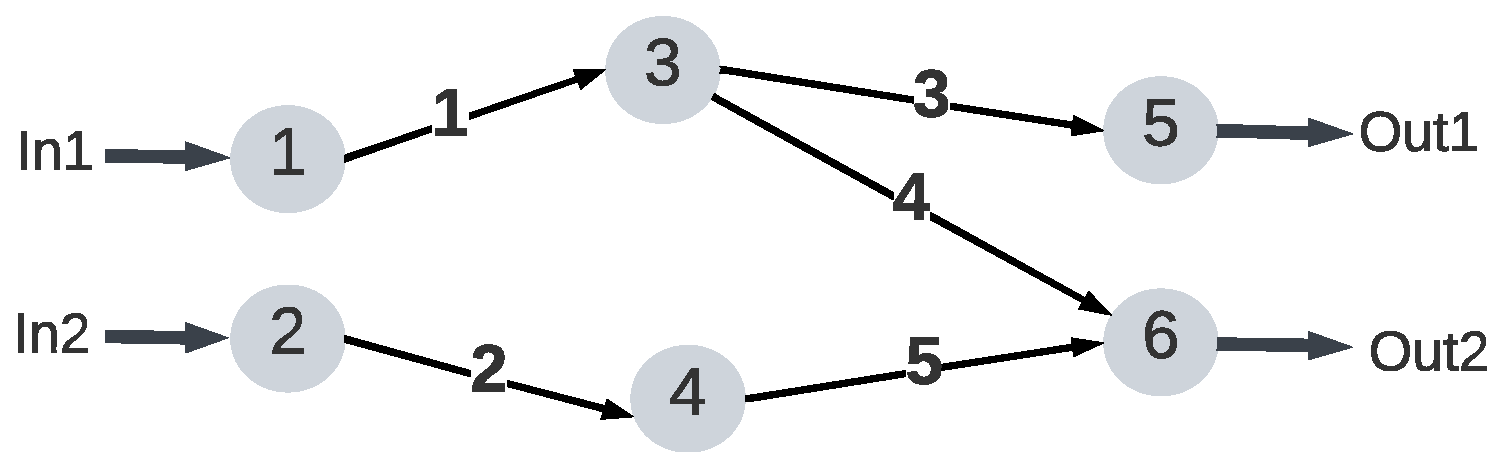
Take Figure 5 as an example to illustrate the modeling process. This communication network comprises six nodes and five links with two input and output streams, respectively. For node 3, the target nodes are nodes 5 and 6, with the node function map as and . Similarly, for node 6, and denote the function corresponding to inputs from node 3 and node 4, respectively. The node function matrix in this system is
is an matrix, indicating the transmission path for each data packet, which can be modeled as follows:
where the superscripts and subscripts refer to the network input and output data streams, respectively. Let be a vector indicating the path from an input l to an output k, then the vector sequence is consistent with columns of F(t). is determined by the following steps:
- Create a null vector representing all the nodes. In this example, the initial is a null vector, as there are two MIMO nodes.
- Trace the transmission paths from the “In-1” to “Out-1”. Then, replace the “In-1” starting node with 1, resulting in .
- Next, replace the following arrival node with the corresponding path function . In this case, the next arrival node is node 3 through the “link-1” path, which corresponds to a function of . Thus, the path vector becomes , where is defined through (11).
- Repeat step 3 until the end node is reached. in this example.
The transmission path matrix in this example will become
Finally, we define the starting node incidence matrix , which indicates the input starting node configuration for each output, as follows:
where is an matrix with . Calculating involves the following steps:
- Generate the initial as a null matrix.
- Columns of correspond to inputs. The first and second columns refer to “In-1” and “In-2”, respectively.
- Rows of refer to the input starting nodes. The first and two rows outline node 1 and node 2, respectively.
- Replace the exact starting node for each input with 1. Hence, the will become
4. Cyber Threat Identification
In this section, the common vulnerabilities of the typical DER cyber layer are identified, followed by attack modeling.
4.1. Cyber Vulnerabilities in CPS
A comprehensive overview of cyber vulnerabilities within the CPS with high DER penetration is summarized in Figure 6 [6,31,32]. Cyberattacks might target either nodes or links. Among the cyber nodes, DERMS and DER clients usually perform strict security policies as the compromised data server may impact multiple devices within the network. However, due to software vulnerabilities or improper security configurations, the possibility of the potential threat still exists. The most common attacks include jamming or denial-of-service (DoS) attacks in order to disable accessibility and replay attacks or false data injection (FDI) attacks aiming to destroy data integrity.
For local controllers, the accessibility policy only allows local communication, and the most common attack is unauthorized access, including control parameters modification, set-point modification, DER disconnection, etc., which is easy to accomplish and may lead to severe consequences.
The most common attack on communication channels is the man-in-the-middle (MITM) attack. Due to existing protocol vulnerability, the attackers may intercept data packets transferred in the channel, which can delay or even drop the packets. Attackers can modify the payload data if there is no or weak cryptographic policy.
The possible consequences of these attacks in the physical layer include increased grid distribution losses, branch overflow, voltage or frequency violation, and stability issues. Note that the latter three may trigger protection devices and lead to load shedding or even blackouts.
Compared to compromising a cyber node, the impact of attacking the channel appears to be limited. Therefore, attacks on nodes are more prevalent. In this study, we primarily focus on node-based attacks.
4.2. Cyberattack Models
To incorporate the CPDS model for impact assessment, the attacks can be portrayed as either the fundamental attacks listed below or through various combinations of these attacks.
4.2.1. Jamming Attack
A jamming attack is implemented by flooding the server buffer with junk packets (i.e., increasing the packet arrival rate v). If v remains below the server processing rate , the server will function, albeit with extended time delays. In contrast, if v surpasses , the superfluous junk packets will rapidly congest the server buffer, leading to the rejection of subsequent incoming packets, thus transforming the jamming attack into a denial-of-service (DoS) attack. Let denote the original cyber variable, as presented before, and denotes the compromised value. The jamming attack can be modeled as
4.2.2. Replay Attack
Replay attacks encompass the retransmission of outdated data packets. Attackers capture data packets previously sent by legitimate sources and subsequently resend these obsolete packets to the intended recipients. Detecting such attacks proves difficult since the outdated data often fall within normal ranges. Consequently, replay attacks can inflict significant disruptions on power grid operations. This type of attack can be depicted using the following equation:
where refers to the time stamp of replacing data packets, which is determined by attackers.
4.2.3. FDI Attack
False data injection (FDI) attacks involve attackers directly altering captured data packet payloads to desired values. This manipulation is usually kept within a feasible range to avoid bad data detection. However, executing an FDI attack requires a more comprehensive understanding of system configuration and background knowledge. The FDI attack can be represented as follows:
The attack signal is usually generated by an external system devised by attackers. This system aims to maximize the impact of the attack while avoiding detection by the bad data detection algorithm, enabling stealthy attacks. Various example systems are discussed in [33,34,35]. Once is established, for linear systems, the compromised node function can be reformulated as follows:
Therefore, by substituting with the original , the FDI attack manifests in the mapping function, and its impact can be estimated by simulating the integrated CPS model. However, pinpointing at a specific time t poses challenges. For risk analysis, a practical approach involves considering the worst-case scenario by assessing the range of . A commonly utilized method entails using the threshold value of the bad data detection algorithm to approximate this range. Nevertheless, it is crucial to acknowledge that this approximation might not comprehensively capture FDI attack characteristics. In FDI-specific research, a more precise model of should be developed.
FDI attacks can impact DER operations in various ways. When FDI targets real or reactive power measurements, it alters the power flow within the system, potentially leading to branch overflow or even necessitating load shedding. However, if the attack targets voltage or frequency measurements, DERs may erroneously adjust terminal voltage or frequency regulation, thereby introducing significant stability issues.
Once the attack type is selected and the corresponding parameters representing the attack capability are determined, the attack model is established and can be integrated into the cyber layer mapping function for impact prediction.
5. Cyberattack Risk Quantification
Risk quantification involves two aspects: impact quantification and attack probability evaluation. In this study, impact quantification is represented by the impact degree , while attack probability is assessed using the attack probability index . The following sections will introduce each aspect in detail, respectively.
5.1. Cyberattack Probability Index
The cyberattack probability index is influenced by two crucial elements: component vulnerability and component criticality [36]. Component vulnerability indicates how easily a component can be compromised, while component criticality emphasizes the potential severity of the consequences if it were to be compromised. In current research, many methods for assessing attack probability focus on component vulnerability, but they may not fully account for nuances in attacker behavior. Launching attacks can lead to physical consequences and trigger alerts to operators, prompting defensive measures that hinder continuous attacks. When a component’s criticality is low, its impact may be limited, causing attackers to perceive their previous efforts as futile. Therefore, attackers often prioritize investigating component criticality before launching attacks to maximize impact. Hence, it is crucial to consider component criticality for accurately modeling attack probability levels.
From the standpoint of attackers, vulnerability pertains to the likelihood of successful attacks, denoted as , while criticality signifies the outcome of those attacks, labeled as . Attackers often prioritize components with substantial outcomes, even if the value is comparatively modest. In order to reflect this subjective preference, a utility function is introduced. Hence, the expected utility of attacking component i, which can be denoted as , can be utilized to quantitatively assess the attack probability, as modeled below:
Therefore, a normalized attack probability index of the ith component, denoted as , can be expressed as
The following sections will introduce the derivations of the likelihood of successful attacks and attack outcome utility , respectively.
5.1.1. Likelihood of Successful Attacks
The probability of a successful attack of node i, which is denoted as , is determined through a Bayesian network. The following steps are employed to compute :
- Assume that node i has K vulnerabilities. Let denote the exploitability score of the kth vulnerability, as defined in the standard vulnerability evaluation system (CVSS). The exploitable probability for the kth vulnerability can be derived by the following equation [37]:
- Let binary variable indicate whether the kth vulnerability is exploited. Thus, the attack condition, denoted as , can be formed as . The likelihood of ith component being compromised under condition can be expressed as,
- Let denote the prior probability of condition . The probability of successful attacks is formulated as
The detailed description can be found in [13].
5.1.2. Attack Outcome Utility
Estimating the precise amount of lost load before executing an attack presents challenges due to the intricate protection and operational strategies in place. An alternative approach is to gauge the impact of an attack on the ith component through its sensitivity, which signifies the change in a physical state variable in response to alterations in the cyber variable . In this study, we choose to employ bus voltages V as the selected state variable, as the voltage is a key factor affecting DER operation status according to IEEE 1547. Consequently, the attack outcome can be quantified using the cyber component sensitivity , representing the ratio of voltage deviation to the cyber variable deviation. It is important to note that the physical layer deviation in this work pertains to bus voltages, which may vary across buses. We select the maximum value as the attack outcome, as shown in the following equation:
where is determined as follows:
where refers to the physical layer input. In this work, it refers to the control command. The first term pertains to the physical system sensitivity, denoting the sensitivity of bus voltage phasors with respect to the control command. To compute physical system sensitivities, we differentiate the complex voltage phasor with respect to a scalar parameter . Consequently, the sensitivities can calculated by solving the following system of equations:
Here, and denote the real and imaginary components of the complex voltage phasor , where represents the complex nodal injections. The index and parameter from (32) correspond to , which represents the control command derived from the control function layer. In the case of the OPF algorithm, the input corresponds to the real and reactive power setpoints of DERs. For the load-sharing algorithm, the input would involve the power at the grid-side PCC or the power ratio of other DERs. It is important to note that these inputs result in differing physical sensitivities. While not explicitly discussed here, the sensitivities in Equation (32) were computed using the QR-decomposition-based algorithm, which enables fast calculations even for a large-scale test case.
The second term in (31) represents the cyber system sensitivity, illustrating how alterations in the communication layer output, influenced by changes in at the ith node, lead to deviations in the physical layer input. Cyber sensitivity is defined based on the preceding mapping function, which can be obtained by the below equation:
where refers to the mapping function from node i to physical layer input. As illustrated in Figure 5, the 1st node cyber sensitivity will be . Finally, the utility function can be defined as follows:
The coefficient reflects the attacker’s subjective preference. Typically, a higher value of indicates a more severe consequence, which tends to be more enticing to attackers, resulting in a higher value.
5.2. Impact Degree
The impact degree quantifies the economic losses stemming from power outages or interruptions triggered by cyberattacks on power grids. This measure can be computed using the following formula:
where refers to the lost load due to compromised component i, refers to the electricity price, and indicates the restoration time. From this equation, it is evident that DER clients or the control center, due to their ability to influence multiple DER units, are susceptible to considerable lost load () when these nodes are compromised, especially when compared to local controllers. Therefore, they inherently face higher risks. Additionally, considering the electricity price (), attacks launched during peak hours, when is relatively high, it can significantly amplify the impact. Notably, differs from traditional physical restoration time as it includes the time required for identifying and recovering the compromised cyber components. From the operator’s perspective, mitigating the potential impact of cyberattacks involves focusing on several defensive measures. Firstly, securing client nodes to reduce their vulnerability to attacks; secondly, organizing reserve or alternative resource capabilities to balance electricity prices between peak and nonpeak hours; and thirdly, actively deploying attack detection algorithms to promptly identify and recover cyber systems from attacks.
In dynamic analysis, determining the lost load can be challenging. However, if attacks lead to stability issues and trigger protection devices, the DERs are highly likely to be disconnected from the main grid. Therefore, the lost DER capacity can be approximated as the lost load in this scenario.
6. Case Study
6.1. IEEE 13-Node Test Case
In the modified IEEE 13-node test feeder, two DERs are integrated at node 680, with capacities of 500 kW and 800 kW, respectively. An additional DER is located at node 692 with a 1000 kW capacity. The DER penetration is about 66%. It is assumed that the power limit of the substation is 500 kW per phase. In normal operations, the substation can be modeled as a traditional slack bus with constant voltage. However, when the power exceeds the limit, the substation voltage will slightly decrease by kW.
Figure 7 illustrates the data flow in the communication layer. In Algorithm 1, the control center calculates the real and reactive setpoints and sends them to each DER, while in Algorithm 2, DER at node 692 adjusts its power injection to control real and reactive power at PCC, and DERs at node 680 use the power ratio of DER at node 692 as input to achieve load sharing. In the following simulation, cases 1, 2, and 3 deploy Algorithm 1, and Algorithm 2 is implemented in case 4. The system dynamic model is implemented in MATLAB 2022, utilizing a machine with the following configuration: an Intel i7 processor with 16 GB of RAM running at 2.8 GHz.
Integrating the VOC-based inverter into the IEEE 13-node test feeder demanded careful consideration due to its low inertia, with minor disturbances risking system instability. Our exploration of inverter operation strategy highlighted potential stability challenges, underscoring the need for real-time monitoring and protection mechanisms to maintain system stability.
6.1.1. Case 1: Modification of Setpoints in OPF Mode
The control command is issued for adjusting the setpoints of DERs. The two DERs at node 680 are considered a unified single unit during the OPF control level. Based on their respective capacities, DER client2 divides and transmits the information to two local controllers, as depicted in Figure 7. Considering the high data processing rate at the control center, the delay time can be disregarded. The communication network parameters are detailed in Table 1, with and representing the processing rate and forwarding rate, respectively. The node function can be characterized as follows:
The functions and correspond to the outputs directed towards nodes 4 and 3, while and represent the outputs to nodes 5 and 6, respectively. As detailed in Section 3, the communication layer outputs, specifically the setpoints of the three DERs, can be described as follows:
Table 2 provides an overview of recent vulnerabilities from NVD that could potentially result in malicious modifications. The probability index for each node is outlined in Table 3. The control center exhibits the lowest vulnerabilities due to its stringent security policy. Comparatively, client1, functioning as a subcenter, employs a more robust security mechanism than client2, resulting in a lower vulnerability. Local controllers, being primarily restricted to local communication, maintain the weakest security policy, rendering them the most vulnerable. Meanwhile, parameter signifies the attacker’s preference. Given the values of found in Table 3, can be determined as follows:
It can be observed that nodes 5 and 6 have the highest probability index, as they are the easiest to compromise and may cause significant voltage variation. Node 2 also has a high probability index, as it can impact all DER setpoints. It is worth noting that the probability index may vary depending on the definition of and .
The impact degree is determined by the worst-case scenario. Taking node 3 as an example, in the worst case, the setpoints were modified to 0 (standby mode), i.e., . The simulation results from the MATLAB model are shown in Figure 8, illustrating the impact of the DER power output attack on voltage variations across all buses. The corresponding DERs are connected to the grid at 3 s (DER 692) and 3.5 s (DER 680_1, DER 680_2), initially staying in the standby state after connection to the primary grid. We observe a minor disturbance in the voltage profile during this stage, attributed to the slight voltage gap between the inverter terminal and grid at the connecting moment. Upon connection to the grid, the DER output power (real/reactive) remains zero while the voltage profile remains unchanged. At 4 s, the control center executes OPF and dispatches real and reactive setpoints to field devices. The DERs’ output ramps up and reaches the desired value at around 5 s, operating at full capacity. Consequently, this also causes a slight elevation in the voltage profile.
Around 7 s, attackers compromise node 3 and reset the setpoints to 0. Consequently, the power output of DER 680_1 and DER 680_2 drops to 0, while DER 692 maintains its output. As a result, to meet the load demand, the power drawn from the substation increases significantly, exceeding the substation’s power limit and causing a voltage decline. Some bus voltages fall below 0.95 p.u., potentially triggering protection mechanisms necessitating load shedding. To maintain voltages within the acceptable range, an optimal load-shedding plan is formulated. This plan involves cutting loads 646, 692, 675a, 611, and 670c, resulting in a total loss of 1172 kW. Assuming that load shedding is initiated at 11 s, the bus voltages subsequently return to the normal range, as illustrated in the figure.
In this paper, we assume and is 24 h [38]. In this case, the risk of node 3 (DER client2) is
The risks associated with each cyber node are presented in Table 4. The result reveals that node 2 carries the highest risk, closely followed by node 1. These nodes can impact all DER units located at bus 680 and 692 simultaneously according to cyberphysical interdependency, thus holding the most significant criticality. Among them, as node 1 is the control center and deploys the strictest security policy, this node is not easy to compromise, making the attack probability of node 1 much lower than node 2. However, considering their high risks, implementing advanced security measures becomes imperative to fortify these specific nodes. Nodes 4, 5, and 6 are local controllers. Their vulnerable levels are comparable. Among them, node 6 holds the highest risk, even higher than node 3. This is due to the high sensitivity (especially the physical layer sensitivity) of this node. Node 4 reveals the lowest risk, as its vulnerability, although noteworthy, is counterbalanced by a less impactful outcome, rendering it less appealing to potential attackers.
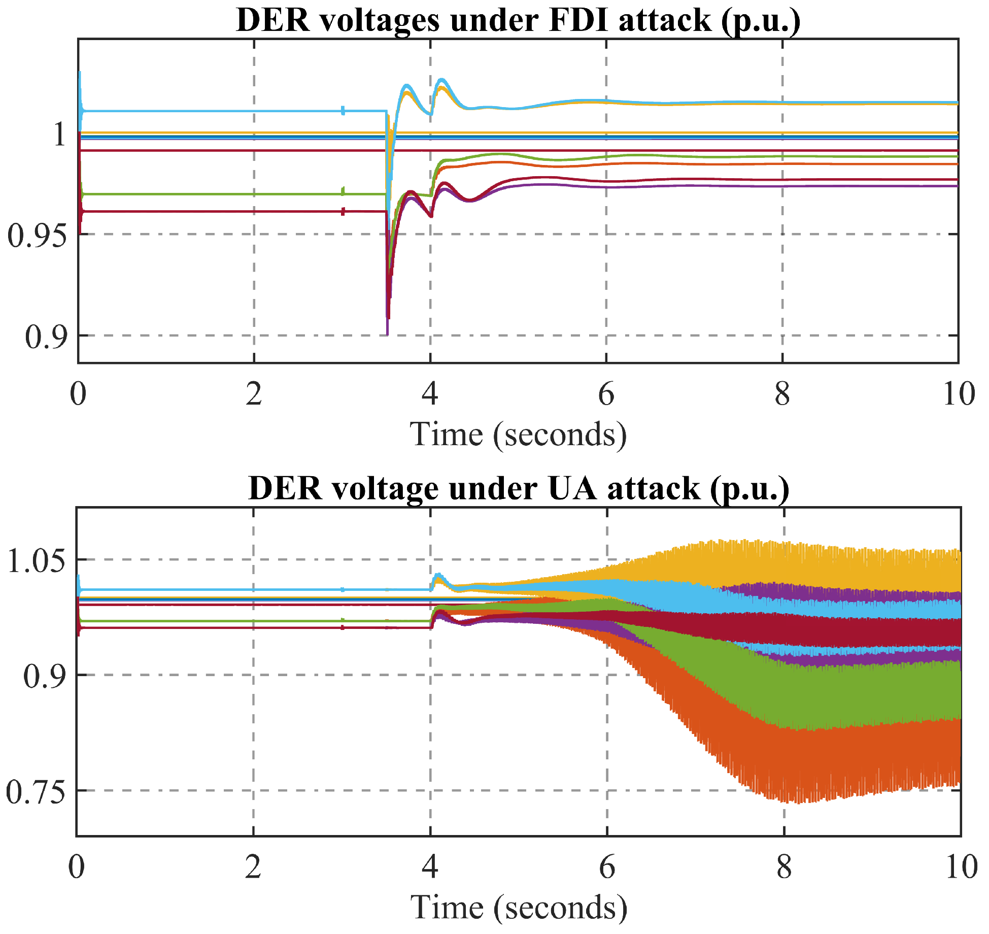
6.1.2. Case 2: FDI Attack on Local Controllers
In this case, attackers try to compromise the local controllers and implement an FDI attack. Assuming the DER operation schedule is the same as in Case 1, attackers compromise node 6 at the beginning and start modifying the local voltage measurement data to 1.2 times the original value, i.e., . This will impact the DER synchronization process. Specifically, as the measurement data are altered, maintaining the same control algorithm, the actual voltage of the inverter tends to be approximately 0.83 times that of the voltage on the grid side. Consequently, at 3.5 s, when the inverter connects to the grid, the significant voltage differential, combined with the low inertia of the inverter, induces an inrush current from the grid into the inverter. This results in a substantial voltage drop on the grid side, as depicted in Figure 9. Following the transition to GFL mode, the inverter aligns with the grid-side voltage, restoring the voltage profile to within normal ranges. However, in practical scenarios, this inrush current may surpass the maximum current limit, triggering protective mechanisms and causing a DER trip.
6.1.3. Case 3: Modification of Local Controller Parameters
In this scenario, the attackers’ aim is to compromise local controllers by manipulating control parameters. Assuming the DER operation schedule remains consistent with previous cases, node 6 is compromised, leading to modifications in the PI controller parameters at the GFL side at 3 s. At this time, the inverter operates in synchronization mode, keeping its performance unaffected and ensuring stable terminal voltage regulation. However, when the DER switches to GFL mode at 4 s, the inverter starts to adjust its output accordingly. Referring to Figure 3, with the inverter initial output at 0, the deviations between the real and reactive power and their setpoints () are notably high. Upon malicious modification of the PI controller, specifically by enlarging its parameters, this disturbance pushes the system out of its stability zone, resulting in detrimental oscillations, as depicted in Figure 9. In practice, this scenario may trigger inverter undervoltage (UV) protection, leading to a DER trip. If not promptly isolated, these significant voltage oscillations may cause further DER trips and potentially lead to load shedding.
6.1.4. Case 4: Jamming Attack in Load-Sharing Mode
In this case, the distribution system operates following Algorithm 2, i.e., the load-sharing algorithm, with the upper-level OPF dictating a setpoint of 1000 kW at the grid-side PCC. In contrast to Case 1, the roles of nodes 2 and 3 were altered as follows:
Here, and refer to the function forwarding to nodes 4 and 3; and refer to the function sending packets to nodes 5 and 6, respectively. The cyber layer outputs become
where refers to the power ratio of DER_1, as depicted in Figure 7. Let us assume that attackers can send junk packets to jam node 6. As a result, whenever the packet arrival rate is comparable to the processing rate, time latency will increase significantly. Assuming that the arrival rate of node 6 becomes 1800/s due to junk packets, the latency becomes approximately 0.01 s. Figure 10 shows the attack consequence. The top and bottom plots indicate an attacked scenario without and with consideration of latency, respectively. It is noted that when considering latency, the jamming attack may lead to an unstable system. However, when the communication latency is ignored, the same jamming attack does not cause system instability. This may lead operators to ignore possible grid oscillations and cause large-scale cascade failure.
6.2. IEEE 123-Node Test Case
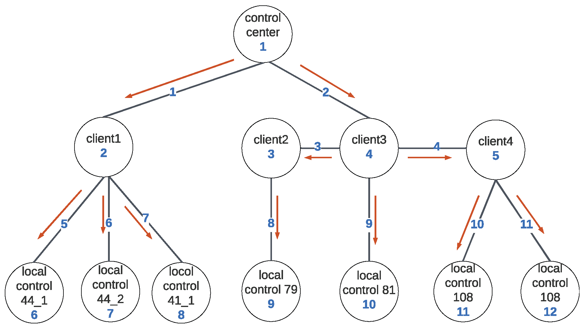
The IEEE 123-node test feeder was modified to incorporate DER units according to the configuration shown in Table 5. The DER penetration level was 80%. We tested the attack scenario involving the modification of real and reactive power setpoints in the control layer when deploying the OPF algorithm. The data flow for this scenario is illustrated in Figure 11. The cyber node risk associated with this test feeder is shown in Table 6.
In this test system, the control center (node 1) presents the highest risk due to its critical role. While not easily compromised, its compromise could impact all DER units, potentially leading to severe load shedding, thus presenting the overall highest risk. While client nodes generally offer higher utility outcomes, they are less vulnerable compared to local controllers. Simulation results exhibit an interspersed pattern among these two types of nodes, as illustrated in the table. Among client nodes, node 4 exhibits the highest criticality as a transfer node, with access to data transmitted to nodes 3 and 5. Despite having the highest probability of attack among all cyber nodes, its impact degree is much lower compared to node 1, positioning it as the second-highest risk if compromised. Node 3 carries the lowest risk among all cyber nodes. It can only affect one DER unit and provides similar outcome utility to the local controller node 9. However, its higher level of security compared to node 9 makes it less attractive from an attacker’s perspective.
It is noteworthy that in comparison to the IEEE 13 node test system, compromising the control center in this highly distributed test feeder yields a similar impact. However, compromising a DER client or a local controller in this system may only affect limited DER capacities, resulting in a significantly lower impact compared to the IEEE 13 node test system. Overall, this distributed system demonstrates greater resilience against cyberattacks than the IEEE 13 node test feeder.
7. Conclusions
The integration of grid-edge inverter-based DERs into distribution grids highlights the necessity for real-time control and monitoring through efficient communication systems. However, this integration of communication networks increases the vulnerabilities susceptible to cyberattackers. As a result, the development of a comprehensive CPS risk assessment framework becomes imperative. In light of limitations in the literature work, this research presents a novel risk assessment framework tailored for distribution grids with substantial penetration of inverter-based DERs. The framework encompasses (i) a detailed distribution grid model that explicitly incorporates the dynamic attributes of inverter-based DERs, (ii) a high-fidelity DER communication layer model that considers communication latency, enabling precise execution of cyber layer attacks, and (iii) a cyberattack risk quantification approach using an attack probability model that factors in both cyber component vulnerability and criticality. Furthermore, the impact of cyberattacks is quantified in terms of economic losses resulting from load shedding. The numerical studies consider various cyberattack scenarios on standard IEEE distribution feeders with grid-edge DERs to validate the framework’s efficacy, affirming its ability to identify high-risk components and guide security policy improvements, thereby contributing to the reinforced system’s reliability and resilience.
Based on the previous discussion, we identified several potential steps to mitigate the cyber risks within the system: (i) Given that high-critical nodes can engender more severe consequences, it is imperative to enhance their security mechanisms to minimize cyber risks. (ii) Recognizing that the degree of impact is assessed based on economic losses incurred from load shedding, it is essential to implement measures such as demand response or augmenting reserve capacity. These actions aim to reduce lost load, particularly during peak hours when electricity prices are relatively high. (iii) Developing a cyber layer restoration strategy is crucial to minimizing post-attack restoration time and mitigating overall risks. (iv) Based on our previous discussion, implementing a high-distributed DER placement strategy enhances system robustness, thereby mitigating system risks.
We observed an increase in emerging cyberphysical coordinated attacks and multistage, multiwave attacks, which are more challenging to detect but can result in more severe consequences. In our future research, we aim to analyze the characteristics of these attacks and develop risk assessment platforms for them. This will enable us to provide guidelines for implementing corresponding defensive strategies and enhancing power system security.
Author Contributions
Conceptualization, W.S.; Methodology, X.G., M.A. and W.S.; Software, X.G. and M.A.; Validation, X.G. and M.A.; Investigation, W.S.; Resources, W.S.; Writing—original draft, X.G. and M.A.; Writing—review & editing, W.S.; Supervision, W.S.; Project administration, W.S.; Funding acquisition, W.S. All authors have read and agreed to the published version of the manuscript.
Funding
This material is based upon work supported by the U.S. Department of Energy’s Office of Energy Efficiency and Renewable Energy (EERE) under the Solar Energy Technology Office (SETO) Award Number DE-EE0009339.
Data Availability Statement
The data presented in this study are available on request from the corresponding author.
Conflicts of Interest
The authors declare no conflict of interest.
References
- Ratnam, K.S.; Palanisamy, K.; Yang, G. Future low-inertia power systems: Requirements, issues, and solutions—A review. Renew. Sustain. Energy Rev. 2020, 124, 109773. [Google Scholar] [CrossRef]
- North American Electric Reliability Corporation. Distributed Energy Resources: Connection Modeling and Reliability Considerations; North American Electric Reliability Corporation: Atlanta, GA, USA, 2017. [Google Scholar]
- Ferreira, P.D.; Carvalho, P.M.; Ferreira, L.A.; Ilic, M.D. Distributed energy resources integration challenges in low-voltage networks: Voltage control limitations and risk of cascading. IEEE Trans. Sustain. Energy 2012, 4, 82–88. [Google Scholar] [CrossRef]
- Kou, G.; Chen, L.; VanSant, P.; Velez-Cedeno, F.; Liu, Y. Fault characteristics of distributed solar generation. IEEE Trans. Power Deliv. 2019, 35, 1062–1064. [Google Scholar] [CrossRef]
- Yang, Q.; Barria, J.A.; Green, T.C. Communication infrastructures for distributed control of power distribution networks. IEEE Trans. Ind. Inform. 2011, 7, 316–327. [Google Scholar] [CrossRef]
- Upadhyay, D.; Sampalli, S. SCADA (Supervisory Control and Data Acquisition) systems: Vulnerability assessment and security recommendations. Comput. Secur. 2020, 89, 101666. [Google Scholar] [CrossRef]
- Qi, J.; Hahn, A.; Lu, X.; Wang, J.; Liu, C.C. Cybersecurity for distributed energy resources and smart inverters. IET Cyber-Phys. Syst. Theory Appl. 2016, 1, 28–39. [Google Scholar] [CrossRef]
- Rahman, A.; Gao, X.; Xie, J.; Alvarez-Fernandez, I.; Haggi, H.; Sun, W. Challenges and Opportunities in Cyber-Physical Security of Highly DER-Penetrated Power Systems. In Proceedings of the 2022 IEEE Power & Energy Society General Meeting (PESGM), Denver, CO, USA, 17–21 July 2022; pp. 1–5. [Google Scholar] [CrossRef]
- Ali, M.; Gao, X.; Rahman, A.; Hossain, M.M.; Sun, W. Emerging Coordinated Cyber-Physical-Systems Attacks and Adaptive Restoration Strategies. In Proceedings of the 2023 IEEE PES Grid Edge Technologies Conference & Exposition (Grid Edge), San Diego, CA, USA, 10–13 April 2023; pp. 1–5. [Google Scholar]
- Liu, X.; Shahidehpour, M.; Li, Z.; Liu, X.; Cao, Y.; Li, Z. Power System Risk Assessment in Cyber Attacks Considering the Role of Protection Systems. IEEE Trans. Smart Grid 2017, 8, 572–580. [Google Scholar] [CrossRef]
- Semertzis, I.; Rajkumar, V.S.; Ştefanov, A.; Fransen, F.; Palensky, P. Quantitative Risk Assessment of Cyber Attacks on Cyber-Physical Systems using Attack Graphs. In Proceedings of the 2022 10th Workshop on Modelling and Simulation of Cyber-Physical Energy Systems (MSCPES), Milan, Italy, 3 May 2022; pp. 1–6. [Google Scholar] [CrossRef]
- He, X. Threat Assessment for Multistage Cyber Attacks in Smart Grid Communication Networks. Ph.D. Thesis, Universität Passau, Passau, Germany, 2017. [Google Scholar]
- Lyu, X.; Ding, Y.; Yang, S.H. Bayesian Network Based C2P Risk Assessment for Cyber-Physical Systems. IEEE Access 2020, 8, 88506–88517. [Google Scholar] [CrossRef]
- Deng, S.; Zhang, J.; Wu, D.; He, Y.; Xie, X.; Wu, X. A Quantitative Risk Assessment Model for Distribution Cyber-Physical System Under Cyberattack. IEEE Trans. Ind. Inform. 2023, 19, 2899–2908. [Google Scholar] [CrossRef]
- Liu, X.; Ospina, J.; Konstantinou, C. Deep Reinforcement Learning for Cybersecurity Assessment of Wind Integrated Power Systems. IEEE Access 2020, 8, 208378–208394. [Google Scholar] [CrossRef]
- Lv, Z.; Han, Y.; Singh, A.K.; Manogaran, G.; Lv, H. Trustworthiness in Industrial IoT Systems Based on Artificial Intelligence. IEEE Trans. Ind. Inform. 2021, 17, 1496–1504. [Google Scholar] [CrossRef]
- IEEE 1547-2018; IEEE standard for Interconnection and Interoperability of Distributed Energy Resources with Associated Electric Power Systems Interfaces. IEEE: Piscataway, NJ, USA, 2018. [CrossRef]
- Xu, L.; Guo, Q.; He, G.; Sun, H. The impact of synchronous distributed control period on inverter-based cyber–physical microgrids stability with time delay. Appl. Energy 2021, 301, 117440. [Google Scholar] [CrossRef]
- Mo, H.; Sansavini, G. Real-time coordination of distributed energy resources for frequency control in microgrids with unreliable communication. Int. J. Electr. Power Energy Syst. 2018, 96, 86–105. [Google Scholar] [CrossRef]
- Xin, S.; Guo, Q.; Sun, H.; Chen, C.; Wang, J.; Zhang, B. Information-Energy Flow Computation and Cyber-Physical Sensitivity Analysis for Power Systems. IEEE J. Emerg. Sel. Top. Circuits Syst. 2017, 7, 329–341. [Google Scholar] [CrossRef]
- Gao, X.; Nejad, R.R.; Sun, W. Decentralized Distribution System Restoration with Grid-Forming/Following Inverter-Based Resources. In Proceedings of the 2022 IEEE Power & Energy Society General Meeting, Denver, CO, USA, 17–21 July 2022; pp. 1–5. [Google Scholar] [CrossRef]
- Meng, W.; Wang, X.; Liu, S. Distributed Load Sharing of an Inverter-Based Microgrid with Reduced Communication. IEEE Trans. Smart Grid 2018, 9, 1354–1364. [Google Scholar] [CrossRef]
- Ali, M.; Ali, M.H.; Gryazina, E.; Terzija, V. Calculating multiple loadability points in the power flow solution space. Int. J. Electr. Power Energy Syst. 2023, 148, 108915. [Google Scholar] [CrossRef]
- Awal, M.A.; Yu, H.; Tu, H.; Lukic, S.M.; Husain, I. Hierarchical Control for Virtual Oscillator Based Grid-Connected and Islanded Microgrids. IEEE Trans. Power Electron. 2020, 35, 988–1001. [Google Scholar] [CrossRef]
- Teng, J.H. A direct approach for distribution system load flow solutions. IEEE Trans. Power Deliv. 2003, 18, 882–887. [Google Scholar] [CrossRef]
- Ali, M.; Dimitrovski, A.; Qu, Z.; Sun, W. A Voltage Inference Framework for Real-Time Observability in Active Distribution Grids. In Proceedings of the 2023 IEEE Power & Energy Society General Meeting (PESGM), Orlando, FL, USA, 16–20 July 2023; pp. 1–5. [Google Scholar]
- Roofegari Nejad, R.; Sun, W. Distributed Load Restoration in Unbalanced Active Distribution Systems. IEEE Trans. Smart Grid 2019, 10, 5759–5769. [Google Scholar] [CrossRef]
- Johnson, J.T. PV Cybersecurity for Hawaii; Sandia National Lab.(SNL-NM): Albuquerque, NM, USA, 2019.
- Roy, A.; Pachuau, J.L.; Saha, A.K. An overview of queuing delay and various delay based algorithms in networks. Computing 2021, 103, 2361–2399. [Google Scholar] [CrossRef]
- Ramaswamy, R.; Weng, N.; Wolf, T. Characterizing network processing delay. In Proceedings of the IEEE Global Telecommunications Conference, 2004. GLOBECOM ’04., Dallas, TX, USA, 29 November–3 December 2004; Volume 3, pp. 1629–1634. [Google Scholar] [CrossRef]
- Amirkhosro, V.; Tamimi, A.; King, A.B.; Majumder, S.; Srivastava, A.K. Cyber–physical vulnerability and resiliency analysis for DER integration: A review, challenges and research needs. Renew. Sustain. Energy Rev. 2022, 168, 112794. [Google Scholar] [CrossRef]
- Hossain, M.M.; Gao, X.; Ali, M.; Rahman, A.; Sun, W. Coordinated Cyber Attacks in Distribution Grid with Distributed Energy Resources: Attacker Perspective. In Proceedings of the 2023 IEEE Kansas Power and Energy Conference (KPEC), Manhattan, KS, USA, 27–28 April 2023; pp. 1–4. [Google Scholar] [CrossRef]
- Chen, X.; Hu, S.; Li, Y.; Yue, D.; Dou, C.; Ding, L. Co-Estimation of State and FDI Attacks and Attack Compensation Control for Multi-Area Load Frequency Control Systems Under FDI and DoS Attacks. IEEE Trans. Smart Grid 2022, 13, 2357–2368. [Google Scholar] [CrossRef]
- Liu, X.K.; Wen, C.; Xu, Q.; Wang, Y.W. Resilient Control and Analysis for DC Microgrid System Under DoS and Impulsive FDI Attacks. IEEE Trans. Smart Grid 2021, 12, 3742–3754. [Google Scholar] [CrossRef]
- Liu, C.; Liang, H.; Chen, T. Network Parameter Coordinated False Data Injection Attacks against Power System AC State Estimation. IEEE Trans. Smart Grid 2021, 12, 1626–1639. [Google Scholar] [CrossRef]
- Kotenko, I.; Chechulin, A. A Cyber Attack Modeling and Impact Assessment framework. In Proceedings of the 2013 5th International Conference on Cyber Conflict (CYCON 2013), Tallinn, Estonia, 4–7 June 2013; pp. 1–24. [Google Scholar]
- Common Vulnerability Scoring System; Forum of Incident Response and Security Teams. July 2022. Available online: https://www.first.org/cvss/ (accessed on 1 March 2024).
- Gao, X.; Chen, Z. Optimal Restoration Strategy to Enhance the Resilience of Transmission System under Windstorms. In Proceedings of the 2020 IEEE Texas Power and Energy Conference (TPEC), College Station, TX, USA, 6–7 February 2020; pp. 1–6. [Google Scholar] [CrossRef]
Figure 1.
Proposed risk assessment framework.

Figure 2.
Architecture of the cyberphysical system.

Figure 3.
The framework of VOC-based inverter control.

Figure 4.
A DER communication network architecture.
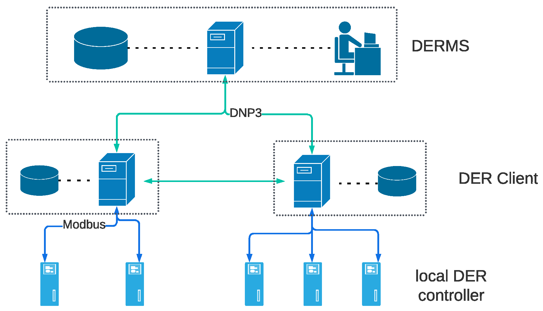
Figure 5.
An example of a communication network.

Figure 6.
An overview of CPS vulnerabilities and possible threats.

Figure 7.
LHS: Data flow in OPF mode; RHS: Data flow in load-sharing mode.
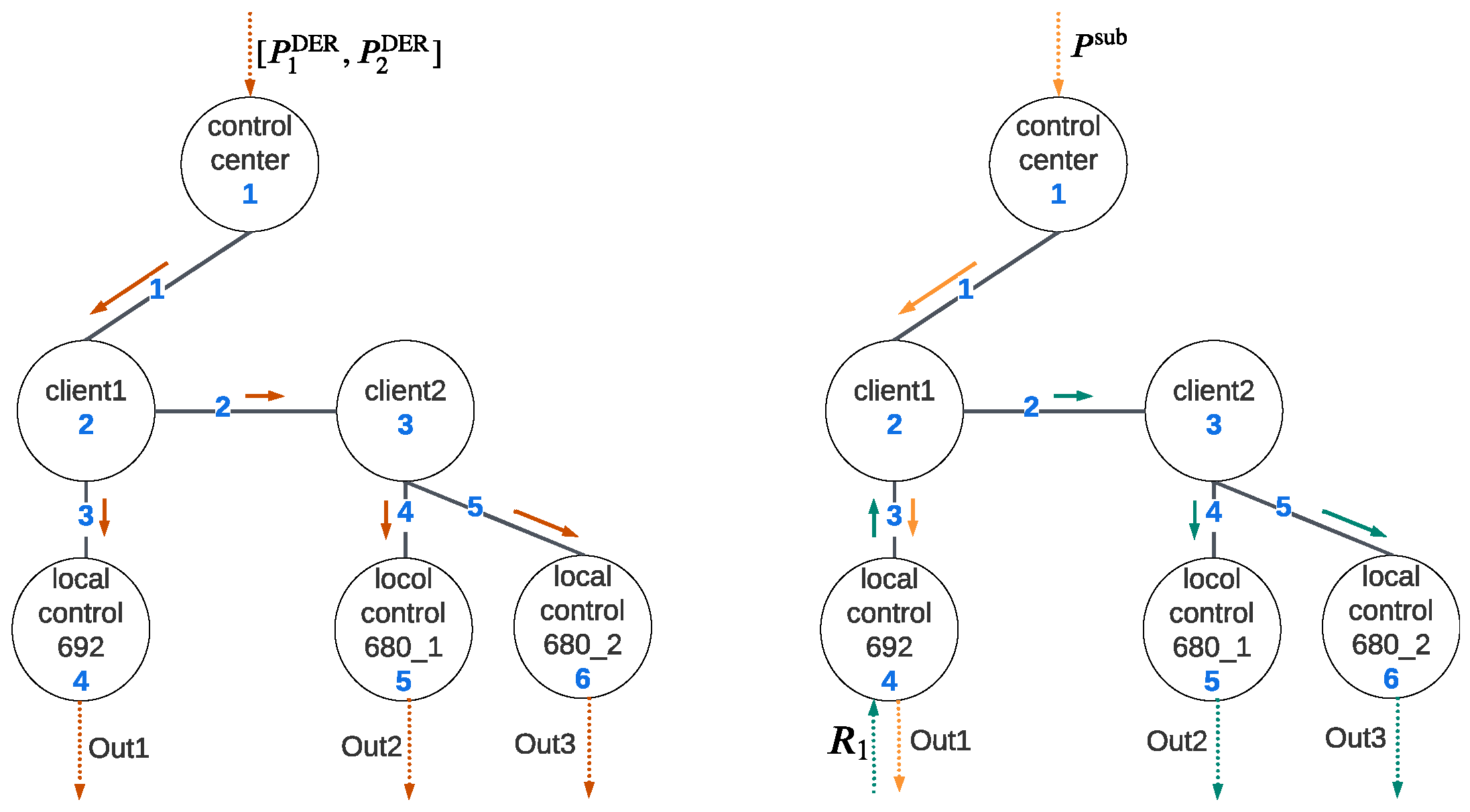
Figure 8.
Case 1: Modification of DER setpoint.

Figure 9.
(Top) (Case 2): FDI attack on local voltage measurement. (Bottom) (Case 3): Modification of local controller parameters.
Figure 9.
(Top) (Case 2): FDI attack on local voltage measurement. (Bottom) (Case 3): Modification of local controller parameters.

Figure 10.
Case 4: Jamming attack on local controller with and without considering communication latency.
Figure 10.
Case 4: Jamming attack on local controller with and without considering communication latency.

Figure 11.
Data flow in OPF mode of IEEE 123-node test system.

Table 1.
Communication network parameters.
| Nodes | Links |
|---|---|
| km | |
| km | |
| k | km |
| k | km |
| k | km |
Note: Propagation speed is km/s.
Table 2.
FDI-related vulnerabilities.
| Vul. No. | Vul. ID | Description | Exploitability Score | Component | Prior Prob. |
|---|---|---|---|---|---|
| 1 | CVE-2021-22803 | Unrestricted Upload of File, could lead to remote code execution of malicious file. | 3.9 | control center | 0.01 |
| 2 | CVE-2020-7545 | Improper Access Control vulnerability that could allow for arbitrary code execution. | 1.2 | control center | 0.02 |
| 3 | CVE-2020-7530 | Improper Authorization vulnerability which allows improper access to executable code folders. | 2.8 | control center | 0.02 |
| 4 | CVE-2020-7532 | Deserialization of Untrusted Data vulnerability could allow arbitrary code execution. | 1.8 | control center | 0.01 |
| 5 | CVE-2022-24312 | Improper Limitation of a Pathname to a Restricted Directory vulnerability exists that could cause modification of an existing file. | 3.9 | control center | 0.01 |
| 6 | CVE-2022-24320 | Improper Certificate Validation Vulnerability. | 2.2 | DER client1 | 0.02 |
| 7 | CVE-2021-22772 | Missing Authentication for Critical Function vulnerability that could cause unauthorized operation when authentication is bypassed. | 3.9 | DER client1,2 | 0.05, 0.1 |
| 8 | CVE-2020-28212 | Improper Restriction of Excessive Authentication Attempts could cause unauthorized command execution. | 3.9 | local controller | 0.1 |
| 9 | CVE-2020-28213 | Download of Code Without Integrity Check vulnerability could cause unauthorized command execution. | 2.8 | local controller | 0.2 |
Table 3.
The attack probability index of cyber nodes.
| Rank | Node | ||||
|---|---|---|---|---|---|
| 1 | 6 | 0.23 | 0.0636 | 0.0146 | 1 |
| 2 | 5 | 0.23 | 0.0636 | 0.0146 | 1 |
| 3 | 2 | 0.061 | 0.102 | 0.0125 | 0.85 |
| 4 | 3 | 0.1 | 0.0636 | 0.0064 | 0.44 |
| 5 | 1 | 0.029 | 0.102 | 0.0059 | 0.4 |
| 6 | 4 | 0.23 | 0.041 | 0.0019 | 0.13 |
Table 4.
Cyber node risks under setpoint modification attack.
| Rank | Node | (kW) | ||
|---|---|---|---|---|
| 1 | 2 | 2037 | 8115.41 | 6898.10 |
| 2 | 1 | 2037 | 8115.41 | 3246.16 |
| 3 | 6 | 530 | 2111.52 | 2111.52 |
| 4 | 3 | 1172 | 4669.25 | 2054.47 |
| 5 | 5 | 298 | 1187.23 | 1187.23 |
| 6 | 4 | 748 | 2980.03 | 387.40 |
Note: Risk values decrease from red to green, indicating lower risk.
Table 5.
DER configuration in 123-node test system.
| DER Location | Number of Units | Capacity per Unit (kW) |
|---|---|---|
| 44 | 3 | 500 |
| 79 | 1 | 400 |
| 81 | 1 | 400 |
| 108 | 2 | 250 |
Table 6.
Cyber nodes risk of IEEE 123-node test system.
| Rank | Node | |||||
|---|---|---|---|---|---|---|
| 1 | 1 | 0.029 | 0.0706 | 0.1501 | 7928.16 | 1190.13 |
| 2 | 4 | 0.061 | 0.0769 | 0.3439 | 2290.8 | 787.88 |
| 3 | 11 | 0.23 | 0.0593 | 1 | 277.78 | 277.78 |
| 4 | 12 | 0.23 | 0.0593 | 1 | 277.78 | 277.78 |
| 5 | 5 | 0.0636 | 0.0593 | 0.2765 | 617.52 | 170.76 |
| 6 | 6 | 0.023 | 0.0228 | 0.0769 | 1494 | 114.88 |
| 7 | 7 | 0.023 | 0.0228 | 0.0769 | 1494 | 114.88 |
| 8 | 8 | 0.023 | 0.0228 | 0.0769 | 1494 | 114.88 |
| 9 | 2 | 0.0636 | 0.0226 | 0.0211 | 2848.56 | 60.04 |
| 10 | 9 | 0.23 | 0.0257 | 0.0867 | 478.08 | 41.44 |
| 11 | 10 | 0.23 | 0.0241 | 0.0813 | 478.08 | 38.86 |
| 12 | 3 | 0.0636 | 0.0257 | 0.024 | 478.08 | 11.46 |
Note: Risk values decrease from red to green, indicating lower risk.
Disclaimer/Publisher’s Note: The statements, opinions and data contained in all publications are solely those of the individual author(s) and contributor(s) and not of MDPI and/or the editor(s). MDPI and/or the editor(s) disclaim responsibility for any injury to people or property resulting from any ideas, methods, instructions or products referred to in the content. |
© 2024 by the authors. Licensee MDPI, Basel, Switzerland. This article is an open access article distributed under the terms and conditions of the Creative Commons Attribution (CC BY) license (https://creativecommons.org/licenses/by/4.0/).
Share and Cite
MDPI and ACS Style
Gao, X.; Ali, M.; Sun, W. A Risk Assessment Framework for Cyber-Physical Security in Distribution Grids with Grid-Edge DERs. Energies 2024, 17, 1587. https://doi.org/10.3390/en17071587
AMA Style
Gao X, Ali M, Sun W. A Risk Assessment Framework for Cyber-Physical Security in Distribution Grids with Grid-Edge DERs. Energies. 2024; 17(7):1587. https://doi.org/10.3390/en17071587
Chicago/Turabian StyleGao, Xue, Mazhar Ali, and Wei Sun. 2024. "A Risk Assessment Framework for Cyber-Physical Security in Distribution Grids with Grid-Edge DERs" Energies 17, no. 7: 1587. https://doi.org/10.3390/en17071587
Note that from the first issue of 2016, this journal uses article numbers instead of page numbers. See further details here.