Reinforcement Learning-Based Energy Management for Fuel Cell Electrical Vehicles Considering Fuel Cell Degradation

Abstract

The service life and fuel consumption of fuel cell system (FCS) are the main factors limiting the commercialization of fuel cell electric vehicles (FCEV). Effective energy management strategies (EMS) can reduce fuel consumption during the cycle and prolong the service life of FCS. This paper proposes an energy management strategy based on the deep reinforcement learning (DRL) algorithm, deep Q-learning (DQL). Considering the unstable performance of conventional DQL during the training process, a new algorithm called Double Deep Q Learning (DDQL) is introduced. The DDQL uses a target evaluation network to evaluate output actions and a delayed update strategy to improve the convergence and stability of DRL. This article trains the strategy using UDDS cycle, tests it using combined cycles UDDS-WLTC-NEDC, and compares it with traditional ECM-based EMS. The results demonstrate that under the combined cycle, the strategy effectively reduced FCS voltage degradation by 50%, maintained fuel economy, and ensured consistency between the initial and final state of charge (SOC) of LIB.

1. Introduction

As the problem of global warming caused by increased carbon dioxide emissions worsens, an increasing number of people are focusing on zero-emission new energy electric vehicles [1]. However, the range limitation and long charging time seriously hinder the commercialization process of electric vehicles [2]. The adoption and utilization of fuel cells present a promising solution for addressing the endurance challenges in EV [3,4].

Fuel cells emerge as a compelling solution to the inherent limitations in electric vehicles, notably their constrained driving range and protracted recharge durations [5]. Compared with lithium-ion batteries, fuel cells exhibit several superior qualities: negligible emissions, an extended driving range, high energy conversion efficiency, and rapid refueling capabilities [6]. The emergence of fuel cell electric vehicles (FCEVs) significantly mitigates the disadvantages of pure fuel cell vehicles, specifically their poor dynamic response and inability to recover braking energy [7]. However, the longevity of the Fuel Cell System (FCS) and hydrogen consumption continue to be major barriers to the widespread use of fuel cell cars. As a result, effective energy management systems are critical for optimizing energy distribution among various power sources.

Current energy management strategies for hybrid and electric vehicles are classified into three types: rule-based, optimization-based, and learning-based strategies [8]. Rule-based energy management strategies, which are often designed in accordance with vehicular driving conditions and the design of the vehicle’s powertrain, are known for their simplicity and practicality, and they typically impose a lower computational burden [9]. However, they are often inefficient and rely significantly on specialist knowledge. Their adaptability to unexpected driving situations is restricted, preventing them from providing ideal control. Furthermore, rule-based techniques frequently display poor transferability and scalability in a variety of environmental scenarios [10].

An increasing number of researchers are focused on optimization-based energy management solutions for hybrid and electric vehicles in order to achieve optimal control and economic efficiency. These tactics are divided into two types: global optimization and instantaneous optimization. Among the many global optimization techniques are Pontryagin’s Minimum Principle, Dynamic Programming (DP) based on Bellman’s theory, Genetic Algorithms, and Particle Swarm Optimization. The DP algorithm is famous for its ability to discover a globally optimal solution and is frequently used as a benchmark for EMS optimization. The DP algorithm, on the other hand, requires prior knowledge of the driving cycle, restricting its flexibility to unpredictable and complex driving conditions [11,12]. Furthermore, its high computing cost limits its use in real-time settings. Strategies such as the Equivalent Consumption Minimization Strategy (ECMS) [13] and Model Predictive Control (MPC) [14,15] have received a lot of interest for instantaneous EMS optimization. ECMS essentially equals the energy consumption of the battery to hydrogen consumption, with the goal of optimizing the energy distribution between the battery and the fuel cell by modifying the equivalent factor. The analogous factor is frequently calculated using specific driving scenarios that may not encompass all driving circumstances. Thus, ECMS optimization uses local optima as a surrogate for global optima. This emphasis on optimization-based solutions shows a substantial shift in research focused at improving energy management efficiency and adaptability in advanced automotive systems.

The optimization algorithms lack self-learning capabilities, which results in insufficient adaptability under a variety of environmental conditions. Learning-based Energy Management Systems (EMS) have acquired extensive use in the optimization of hybrid vehicle systems due to the rapid growth of artificial intelligence technologies. Zheng proposed an energy management strategy combined with working conditions identification [16]. Zhou et al. presented an adaptive energy management strategy, including a driving pattern recognizer and a multi-mode model predictive controller. The result showed that compared to a single-mode benchmark strategy, the proposed multi-mode strategy could reduce at least 2.07% hydrogen consumption [17]. Reddy introduced an intelligent PEMS employing reinforcement learning, facilitating real-time learning of optimal strategies through interaction with the onboard power system [18]. Sun and Fu proposed an energy management strategy grounded in reinforcement learning, leveraging ECMS for heightened computational efficiency, minimized fuel cell power fluctuations, and optimized fuel economy in FCEVs [19]. Fu integrated the DRL and equivalent power minimization strategy framework to optimize FC and BAT power allocation, ensuring FC’s efficient operation and reducing hydrogen consumption [20]. Li introduced an energy management strategy for hybrid battery systems, considering battery cell and heat cell characteristics, with the aim of minimizing energy loss and enhancing the overall system’s electrical and thermal safety levels [21].

Recently, numerous studies have investigated energy management strategies considering fuel cell performance degradation. Wang et al. quantified the degradation process of fuel cells using a simple electrochemical model. The degradation process of fuel cells was characterized by the decay of the electrochemical surface area under transient power load, start-stop cycle, idle condition, high-power load, and other operating conditions. A deterministic dynamic programming algorithm was employed to optimize the energy management process and extend the service life of fuel cells [22]. Song proposed a power adaptive adjustment strategy during the degradation process based on the fuel cell models established under different health states, aiming to achieve higher energy efficiency throughout the entire lifespan of the fuel cell [23]. Sun et al. proposed an energy management strategy based on game theory, quantifying the distinct preferences of each energy source and utilizing the Nash equilibrium to reconcile the preferences among different energy sources [24]. Zhang et al. employed a wavelet-based control strategy to optimize the efficiency and durability of fuel cells in real time [25]. The above methods all aim to optimize lifespan degradation using traditional optimization or rule-based methods.

The present corpus of research focuses mostly on the fuel economy of FCEV and misses the influence of fuel cell deterioration on power allocation. In addition, the application of deep reinforcement learning in energy management strategies is relatively scarce.

To further explore the effectiveness of reinforcement learning in energy management strategies, this research proposes a deep reinforcement learning (DRL)-based energy management technique that takes fuel cell longevity into account. The key contributions of this study are as follows:

• The creation of a DRL-based energy management system is intended to optimize hydrogen usage while maintaining battery SOC stability. It uses deep reinforcement learning skills to adapt to changing driving situations and vehicle states.
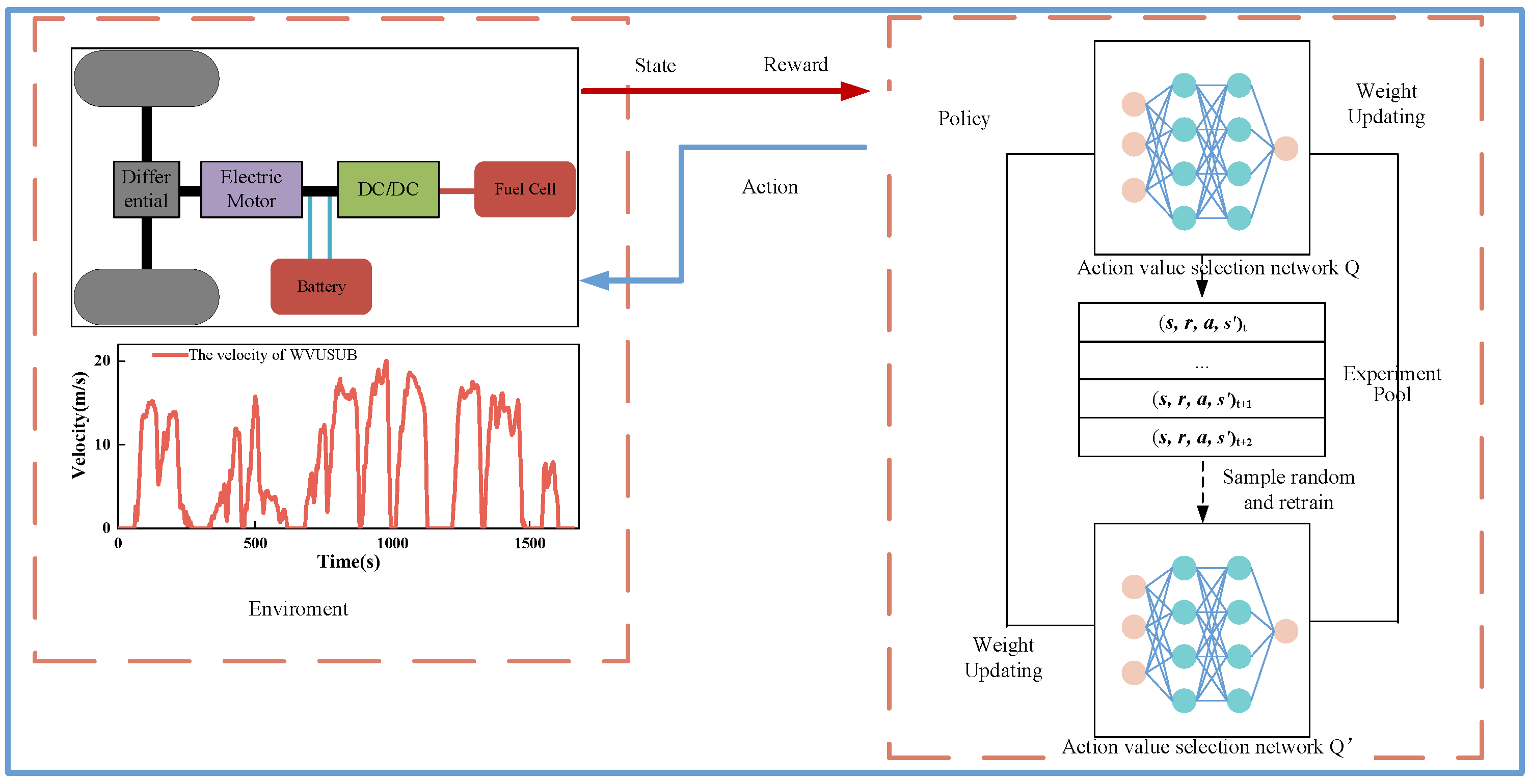
• Double Deep Q-learning (DDQL) implementation: DDQL is used to manage the energy of fuel cell electric vehicles (FCEVs). This approach estimates Q-values using two distinct neural networks, avoiding the overestimation problem associated with a single network. This dual-network technique improves the learning process’s accuracy and dependability.
• Incorporation of FCS degradation into energy management: The incorporation of Fuel Cell System (FCS) degradation factors into the energy management strategy is a novel component of this study. The DDQL structure does this by establishing a balance between fuel economy and FCS longevity.
• Validation employing standard drive cycles: The performance of the proposed technique is further confirmed by employing several standard driving cycles. These experiments indicate the strategy’s robustness in a variety of driving circumstances, including those not seen during training.

Overall, this work proposes a comprehensive approach to energy management in FCEVs, combining the most recent AI-driven approaches with actual vehicle dynamics and fuel cell degradation issues. The findings indicate potential in terms of improving the efficiency and durability of FCEVs.

The organizational structure of this article is as follows. The first chapter introduces the research background and existing energy management strategies, highlighting their limitations. The second section outlines the powertrain structure of the FCEV, FCS, and LIB models, as well as the principle of FCS degradation. Subsequently, Section 3 delves into optimization algorithms and presents an energy management strategy based on deep reinforcement learning tailored to the objectives of this study. Section 4 provides a comprehensive analysis of the training process and simulation results of the energy management strategy, alongside a comparative analysis with benchmark algorithms for verification, which is summarized in Section 5.

2. The Powertrain of the FCEV Model

In order to study energy management strategy, the model of FCEV powertrain based on actual vehicles is proposed. Figure 1 shows the topological structure of FCEV. The main parameters of FCEV are presented in

Table 1. The parameters of the studied FCEV.

Component	Parameters	Value
FCEV	Mass	1070 kg
	Wheel rolling radius	0.466 m
	Coefficient of rolling resistance	0.00863
	Air drag coefficient	0.335
	Equivalent windward area	2.06 m2
FCS	Rated power	50 kW
Lithium-ion Battery	Capacity	20.6 Ah
DC/DC	Fixed efficiency	0.98
DC/AC	Fixed efficiency	0.95

. The powertrain primarily consists of fuel cells and LIB, with FCS predominantly supplying power during driving and LIB serving as auxiliary power sources. The FCS supplies power through a unidirectional DC/DC converter and manages the state of charge (SOC) of the LIB. A bidirectional DC/DC converter is utilized to capture braking energy and supply power for vehicle operation.

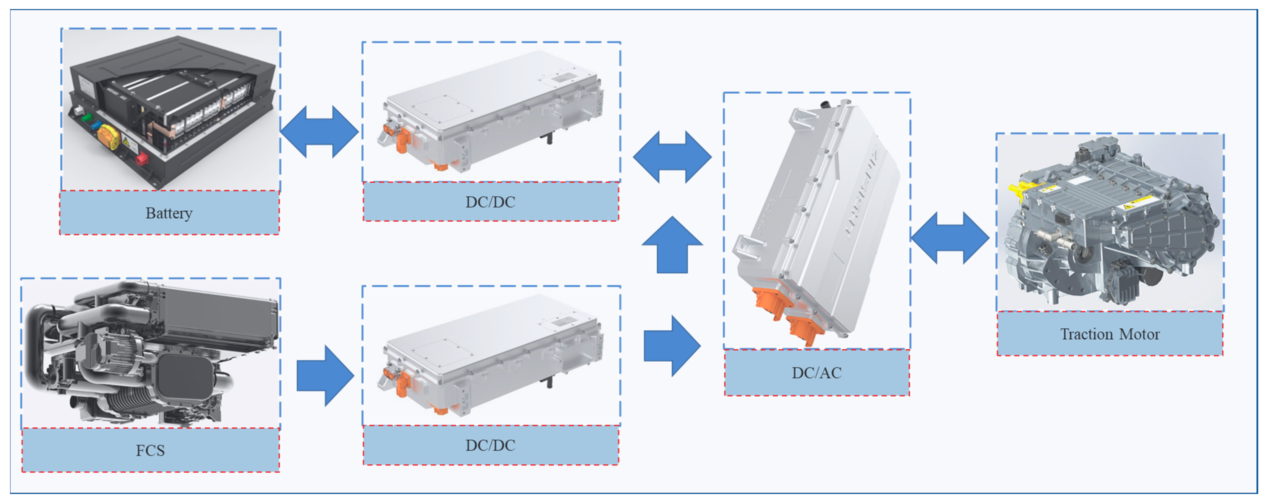
2.1. System Configure

The vehicle model is employed to calculate the power required by the powertrain during vehicle operation [21]. The required power P_wheel is a function of the vehicle speed v, given by the following equation:

$$P_{wheel}=\left(mg\sin \alpha +\delta m\frac{du}{dt}+\frac{1}{2}\cdot C_{D}A\rho v^2+mgf\cos \alpha \right)\cdot v$$

(1)

where m is the mass of vehicle, g is the gravity acceleration, C_D is the coefficient of air resistance, ρ is the density of the air, and f is the rolling resistance of the vehicle. The total power balance equation is given by:

$$P_{req}=\frac{P_{wheel}}{{\eta }_{DC/AC}{\eta }_{\mathrm{motar} }{\eta }_{\mathrm{trans} }}=P_{fc}{\eta }_{DC/DC}+P_b{\eta }_{DC/AC}$$

(2)

where η_DC/DC the efficiency of the DC/DC converter in the formula. The efficiency of the DC/AC converter is represented by η_DC/AC, the efficiency of the motor is represented by η_motor, and the efficiency of the transmission system is represented by η_trans. P_fc denotes the net output power of the fuel cell system, and P_b denotes the output power of the lithium battery.

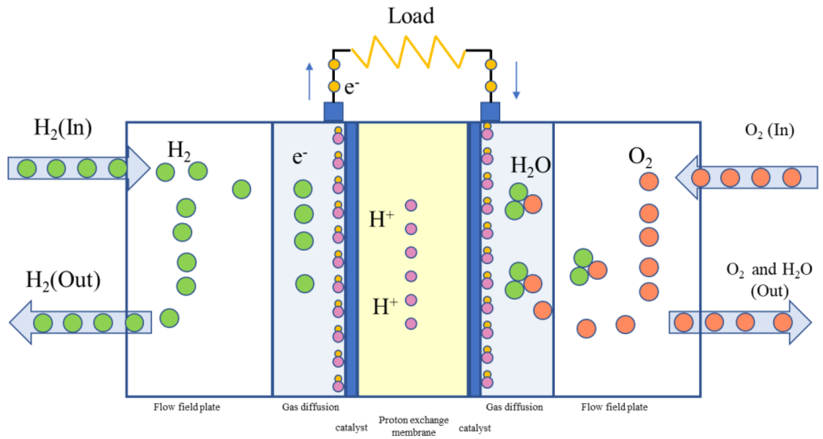
2.2. Fuel Cell System

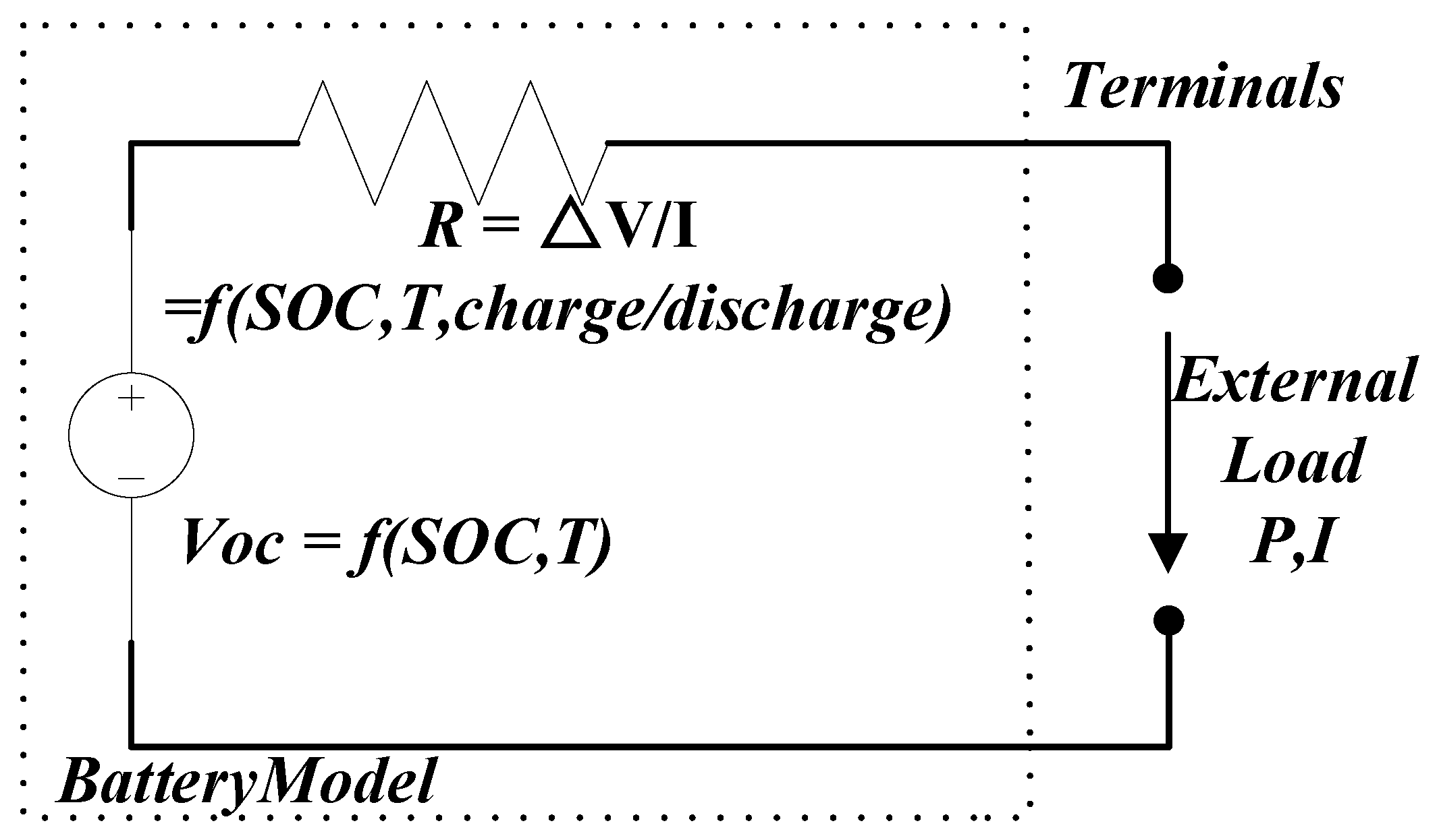
As the main power source of the FCEV, PEMFCS generates electrical energy through the reaction of hydrogen and oxygen, as is shown in Figure 2. During vehicle operation, the EMS controls the output of the FCS and keep it operating properly. This study uses a PEMFCS with a rated power of 50 kW. The output voltage model of PEMFCS is based on a semi-empirical equation, suggested by Mann et al. [26]. The output voltage of a single cell can be calculated by the following equation:

$$V=E_{\mathrm{nernst} }-V_{act}-V_{\mathrm{ohm} }-V_{\mathrm{con} }$$

(3)

$$E_{\mathrm{nernst} }=E_0-\frac{\Delta S}{2F}(T_{st}-T_0)+\frac{R{T}_{st}}{2F}\left(\ln P_{H_2,an}+\frac{1}{2}\ln P_{O_2,ca}\right)$$

(4)

$$V_{act}={\xi }_1+{\xi }_{2}T+{\xi }_{3}T\ln I+{\xi }_{4}T\ln \left(C_{O_2}\right)$$

(5)

$$C_{O_2}=0.197\cdot P_{o_2,ca}\cdot \exp \left(\frac{498}{T}\right)$$

(6)

$$V_{ohmic}=i{R}_i$$

(7)

$$V_{con}=-B\ln \left(1-\frac{i}{i_{lim}}\right)$$

(8)

where E₀ is the standard state reference potential; and T₀ is the standard state temperature, 298.15 K; The entropy change is denoted by ΔS. R denotes the gas constant. Faraday’s constant is F. T_st denotes the stack temperature; ξ₁, ξ₂, ξ₃, and ξ₄ are semi-empirical constants. The stack current is denoted by I. C_O2 represents the oxygen concentration on the surface of cathode catalyst. R_i denotes internal resistance. Hydrogen consumption m_H2 is related to the net fuel cell output power P_fc, which can be shown as follows:

$$m_{H_2}=\frac{n_{st}I}{2F}{M}_{H_2}$$

(9)

where n_st represents the numbers of cells; F is the constant of Faraday; and I_st represents the stack current. Therefore, the efficiency of fuel cell stacks is as follows:

$$\left\{\begin{array}{l}{P}_{fc}=n_{st}VI-P_{aux}\\ {\eta }_{fc}=\frac{n_{st}VI-P_{aux}}{m_{fc}LH{V}_{H_2}}\end{array}\right.$$

(10)

where V_st represents the cell voltage, and P_aux represents the accessories consumption power, such as air compressor, hydrogen circulation pump and cooling water pump, etc. LHV_H2 represents the low calorific value of hydrogen, and the relationship between total power of FCS and the efficiency is depicted in Figure 3.

The degradation of a fuel cell is mostly caused by changes in external working circumstances, which cause extreme swings in response conditions such as the temperature, humidity, and pressure inside the stack. A fast load change, high power load, and other working conditions are the most influential working conditions. As a result, the fuel cell degradation rate model is used in this work to assess the energy management strategy’s life extension efficacy [27].

$$\Delta {\varphi }_{\mathrm{dr}}=k_p\left(k_1{t}_1+k_2{t}_2+k_3{t}_3\right)$$

(11)

where Δϕ_dr represents the aging rate after cyclic working conditions, and k_p represents the correction coefficient, which is used to measure the difference between the experimental situation and the simulation situation. t₁, t₂, and t₃ indicate the idle time of fuel cell, big load change duration, and large load duration, respectively; while k₁, k₂, and k₃ represent the degradation coefficients corresponding to the three categories. The parameters of PEMFC are shown in the

Table 2. The parameters of the studied FCS.

Parameters	Value	Parameters	Value
E0	1.229 V	kp	1.47
ξ1	−0.995	k1	0.00126 (%/h)
ξ2	2.1228 × 10−3	k2	0.0000593 (%/h)
ξ3	2.1264 × 10−5	k3	0.00147 (%/h)
ξ4	−1.1337 × 10−4	LHVH2	242 kJ/mol
B	0.497

.

2.3. Li-Ion Battery

This article establishes a one-dimensional numerical model of LIB using the Rint model. Figure 4 illustrates the equivalent circuit diagram of the model.

The voltage loop equation of the power battery is depicted in the following equation.

$$\left\{\begin{array}{l}{P}_b=U_b{I}_b\hfill \\ U_b=E-I_b{R}_b\hfill \end{array}\right.$$

(12)

$$I_b=\frac{E-\sqrt{E^2-4R_b{P}_b}}{2R_b}$$

(13)

In the formula, P_b, U_b, I_b, E, and R_b represent output power, output voltage, LIB current, open-circuit voltage, and internal resistance, respectively. According to the relationship between the ohmic charge-discharge resistance and open-circuit voltage of the power battery under different SOC values, the relationship between the characteristics of the power battery pack and the state of charge (SOC) was calculated under different SOC values. The internal resistance during charging and discharging is shown in the following equation.

$$R_{\mathrm{int}}=\left\{\begin{array}{c}{R}_{dis}\begin{array}{cc}when& P_b\le 0\end{array}\\ R_{chg}\begin{array}{cc}when& P_b>0\end{array}\end{array}\right.$$

(14)

Among these variables, R_dis and R_chg denote discharge resistance and charging resistance, respectively. Figure 5 illustrates the correlation between state of charge and each open-circuit voltage. The data were sourced from experimental tests conducted by the National Renewable Energy Laboratory (NREL) [28].

The state of charge (SOC) of LIB is a crucial control parameter in energy management strategies. In this study, the SOC was computed by the ampere-hour integration method.

$$SOC(t)=SO{C}_0-\frac{{\eta }_b{\displaystyle {\int }_0^t{I}_b}(\tau )d\tau }{Q_b}$$

(15)

where SOC(t) represents the current SOC value of the lithium battery, and SOC₀ represents the initial SOC value of the lithium battery, η_b represents battery efficiency, and Q_b represents the rated capacity of a lithium battery.

3. Design of DDQL-Based EMS Considered the Performance Degradation of FCS

The Double DQL algorithm is applied to the FCEV energy management strategy. In this section, the fundamental concepts of reinforcement learning and the proposed Double DQL energy management strategy are introduced.

3.1. The Algorithm of DQL

The Deep Q-learning (DQL) algorithm is a breakthrough in the field of reinforcement learning (RL) that combines Q-learning, a traditional RL algorithm, with deep neural networks. This approach allows the handling of high-dimensional state spaces, which is a significant challenge for classical RL methods. Here is an overview of DQL’s fundamental principles.

According to the current state s of the environment, an agent executes action a according to a policy defined for the environment. Simultaneously, the agent receives a reward R for the action and transitions to a new state s′ within the environment. Using this feedback, the agent updates its policy, aiming to find the policy π that maximizes the action-value function. Thus, the action-value function, also referred to as the Q-function, represents the expected discounted sum of rewards.

$$Q^{\pi }(s,a)={\displaystyle \sum _{t=0}^{\infty }\left\{{\gamma }^{t}R\left(s_t,a_t\right)\Vert s_0=s,a_0=a\right\}}$$

(16)

where R is the single-step reward, and γ in the range of [0, 1], representing the discount factor to future reward values. The Q function represents the cumulative value of the long-term expected reward and is utilized to evaluate the benefits of taking action a under the state s. The optimal Q function Q* can be defined as:

$$Q^{*}(s,a)={\max }_{\pi }{Q}^{\pi }(s,a)$$

(17)

And thus, the strategy can choose action a by:

$$a=\underset{a\in A}{\mathrm{argmax}}{Q}^{*}(s,a)$$

(18)

And then the action value can be renewed to:

$$Q_{t+1}(s_t,a_t)=Q_t(s_t,a_t)+\alpha \left[R_{t+1}+\gamma \underset{a\in A}{\max }{Q}_{t+1}(s_{t+1},a_{t+1})-Q_t(s_t,a_t)\right]$$

(19)

The experience pool is established to store the data required by the neural network. In this study, the form of experience pool in this research is quadruplet (s, a, r, s′), which comprises the current state s, the agent’s action a, the immediate reward r after executing the action, and the state at the next moment s′. To mitigate correlations in the data derived from the driving cycle, the experience replay method is employed to smooth over changes in the data distribution and reduce training difficulty.

3.2. The Energy Management Strategy Design of Double-DQL

The Double Deep Q-learning (Double DQL) algorithm is an improvement to the original Deep Q-learning (DQL) technique that addresses the issue of overestimation in the Q-learning algorithm. The action network and target network can be decoupling by the Double Deep Q-learning network. The action network is used for selecting actions and the target network is used for evaluating the value of the current state. The actor network updates the weights value at each step, while the target value updates the weight on every τ step. When updating the target value, the action corresponding to the maximum action value function from the action network is chosen, and then it is used as the action indicator of the target network to determine the action value function of the target network. The weight parameters of target network are overwritten by the actor network. And the network parameters are updated by the loss function as follows:

$$L\left({{\theta }_t}^{\prime }\right)=E\left[{\left(y_t-Q\left(s_t,a_t;{{\theta }_t}^{\prime }\right)\right)}^2\right]$$

where y_t presents the optimization target.

$$y_t=R_{t+1}+\gamma Q\left(s_{t+1},\underset{a}{\arg \max }Q\left(s_{t+1},a;{\theta }_t\right);{{\theta }_t}^{\prime }\right)$$

The exact procedures of DDQL algorithm in this paper are shown in Algorithm 1. And the process of the energy management strategy based on DDQL algorithm is presented in Figure 6. The whole simulation progress, including energy-consumption system modeling, vehicle dynamic modelling, and reinforcement agent modelling, is realized in MATLAB 2023.

The state space [V_spd, V_acc, SOC] of reinforcement learning primarily encompasses four variables: the state of charge of LIB, the current vehicle speed, the current acceleration, and the current output power of FCS.

The control variable utilized in this study is the output power of FCS [P_fc], ranging from a maximum output power of 50 kW to a minimum output power of 0 kW.

The design of the reward function directly impacts the convergence of the reinforcement learning process. Consequently, this study meticulously examines the reward function. The objective of this study is to minimize hydrogen consumption and prolong the lifespan of fuel cells while ensuring the consistency of the initial and final state of charge (SOC) of LIB. Hence, a reward function is devised based on these three factors. The formulated reward function is as follows:

$$R=\left\{\alpha \frac{dFuel}{dt}+\beta {(SO{C}_{ref}-SOC)}^2+\lambda {\varphi }_{\mathrm{deg}}\right\}$$

(20)

where R is the immediate reward for taking action a in state s to state s′; Fuel represents hydrogen consumption; and ϕ_deg represents the rate of the fuel cell degradation.

Algorithm 1: Double Deep Q-learning.

Parameters: A, Initialize replay memory D with capacity N. Initialize action-value evaluating function Q with random weights ${\theta }^{-}$. Initialize target action-value function Q∧ with weights ${{\theta }^{-}}^{\prime }={\theta }^{-}$. for episode = 1:max(episode) do   for t = 1:max(during time) do     With probability ε select a random action a;     otherwise, select $a_t=\underset{a}{\mathrm{argmax}}Q(s_t,a;{\theta }^{-})$     Execute action a with environment and observe reward Rt and next state st+1.     Store transition $(s_t,a,R_t,s_{t+1})$ in D.     Sample random minibatch of transitions $D={\displaystyle {\sum }_{i=1}^n(s_t,a_t,R_t,s_{t+1})}$ from D.     For t = 1, n do     Set: $y_t=\left\{\begin{array}{c}{R}_t if episode ends at step t+1\\ R_{t+1}+\gamma Q\left(s_{t+1},\underset{a}{\mathrm{argmax}}Q\left(s_{t+1},a;{\theta }_t\right);{{\theta }_t}^{\prime }\right) otherwise\end{array}\right.$     Perform gradient descent step on $\left[{\left(y_t-Q\left(s_t,a_t;{\theta }_t^{-}\right)\right)}^2\right]$ update the selection network.     Every τ step reset ${{\theta }^{-}}^{\prime }= {\theta }^{-}$, update target network   end for end for

4. Result and Discussion

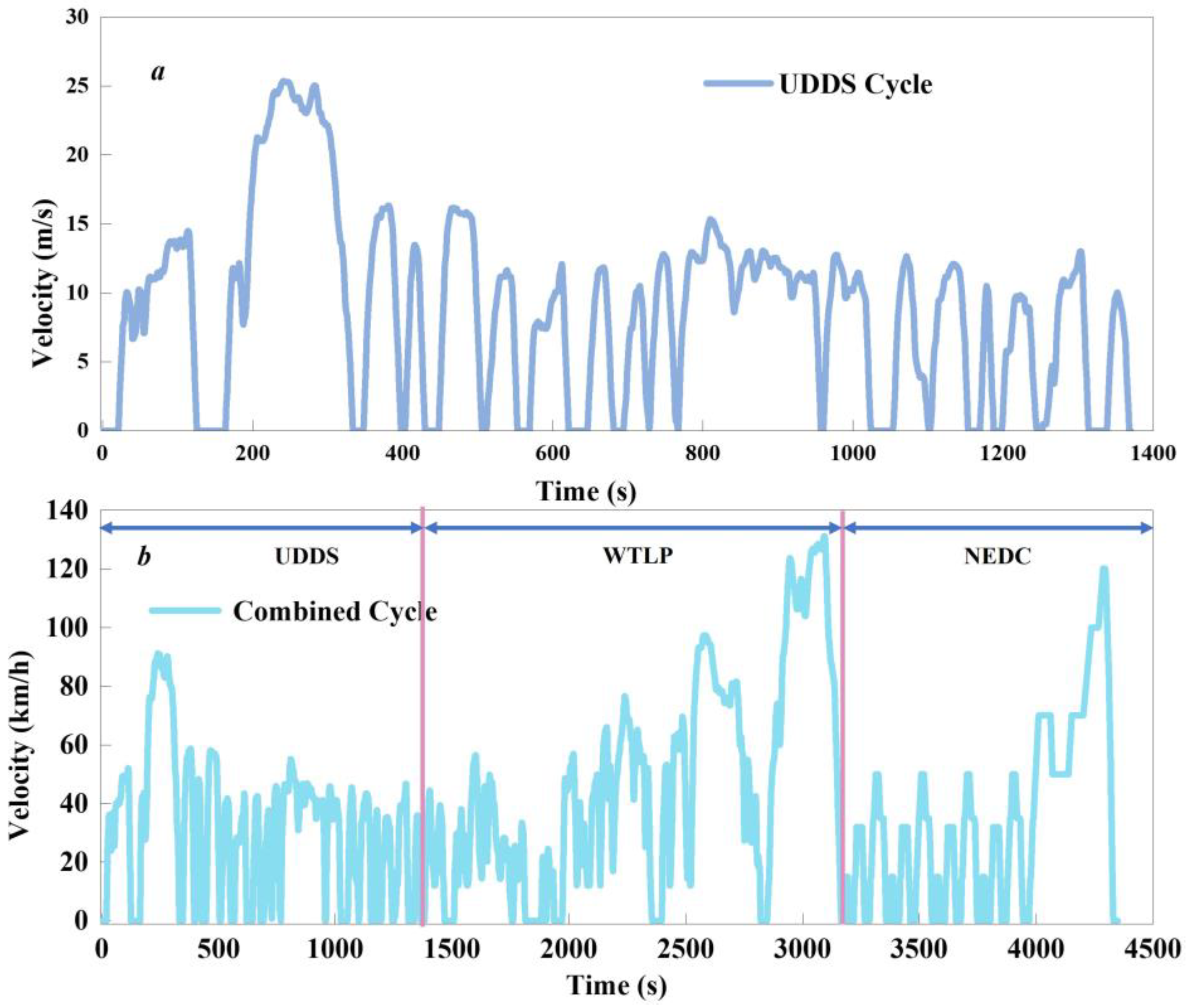
4.1. Training Setting

The Urban Dynamometer Driving Schedule (UDDS), New European Driving Cycle (NEDC), and World Light-duty Vehicle Test Procedure (WLTP) were used to train and test the DDQL-agent, as shown in Figure 7. The detailed cycle information of speed profile is listed in

Table 3. The detailed cycle information of three different cycles.

Cycle	Speed Max (km/h)	Average Speed (km/h)	During Time (s)
UDDS	91.25	31.5	1370
WLTP	131.3	46.5	1800
NEDC	120	24.71	1180

. The DDQL-based agent was trained with the speed profile of the UDDS dataset. To validate the performance of the suggested strategy in different cycles, three datasets of speed profiles were combined into a testing cycle (UDDS-WLTP-NEDC) as shown in Figure 7b.

Table 4. The parameter settings of DDQL.

Parameters	Value	Parameters	Value
Learning rate	0.001	Sample batches size	64
Layers of neural network	3	α	4.4
Discount factor	0.99	β	2000
Experience pool capacity	10,000	λ	5000

lists detailed training parameter settings for the DDQL-agent. And the training process of DDQL-agent was executed on the computer with an NVIDIA GeForce RTX 2070 SUPER.

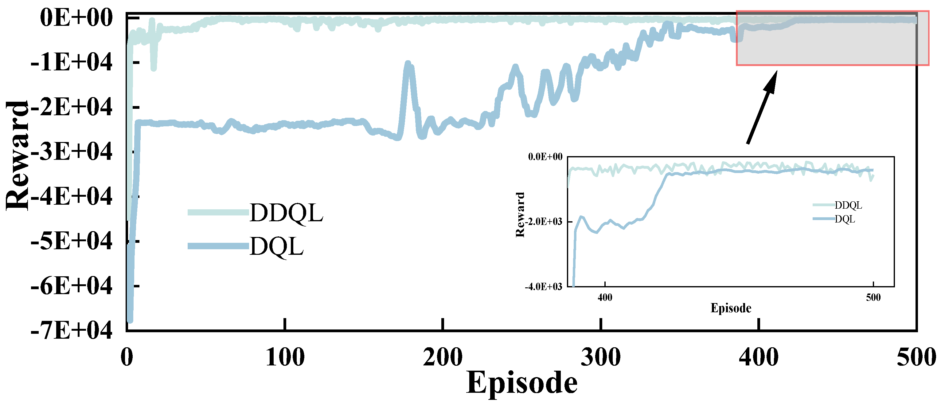
4.2. Training Performance Comparison

Figure 8 presents the evolution of cumulative rewards during the training iterations based on two strategies, DQL- and DDQL-based strategies, under the UDDS cycle. Every item in the reward function was multiplied by a negative value, so the cumulative reward was negative value. It indicates the smaller the cumulative reward, the farther away it is from the target value. The closer the cumulative reward is to 0, the closer the training result is to the target.

In the initial stage of training, the exploration rate was set to 1, enabling the agent to explore various unknown states with a wide range of actions. Consequently, the cumulative reward remained low and exhibited significant fluctuations. However, after approximately 200 episodes, the reward increased with the exploration rate decline to 0.134 as the number of training sessions increased. Consequently, the agent’s training stabilized, leading to a propensity to choose actions associated with smaller penalties.

By around 420 episodes of training, the exploration rate approached 0.01, and both strategies converged to a stable state, characterized by a noticeable enhancement in cumulative rewards compared to their initial performance. Notably, compared to the DQL-agent, the DDQL-agent could achieve convergence faster and obtained higher cumulative rewards. This superiority can be attributed to DDQL’s utilization of two networks, effectively avoiding action overestimation and ensuring more stable cumulative rewards during training. These findings underscore the superior outcomes achieved by the proposed DDQL methodology.

4.3. Optimality of DDQL-Based EMS

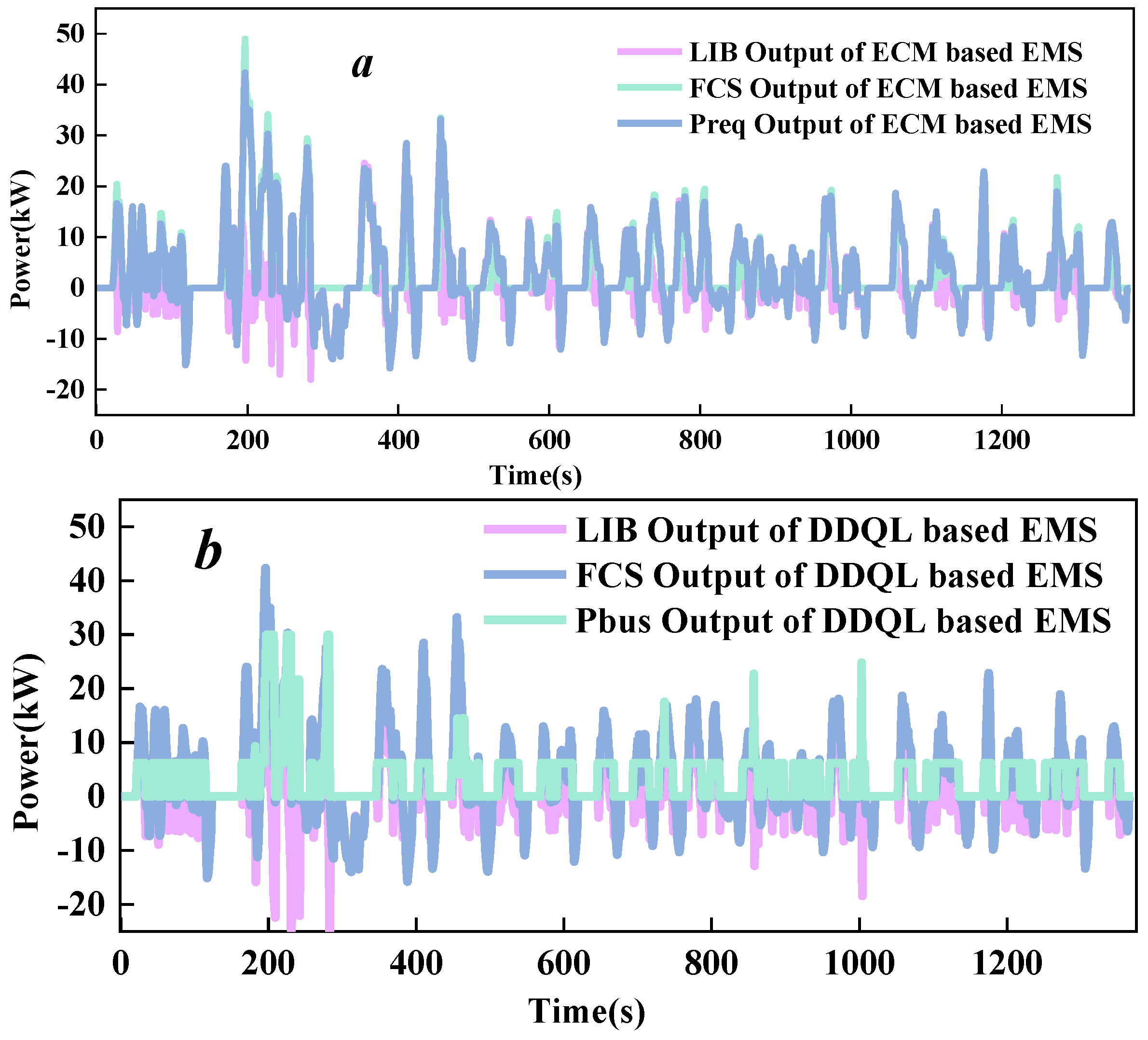
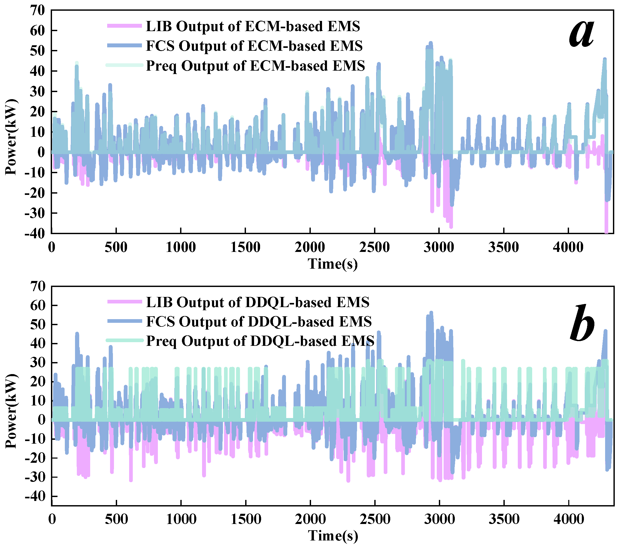
4.3.1. Power Distribution

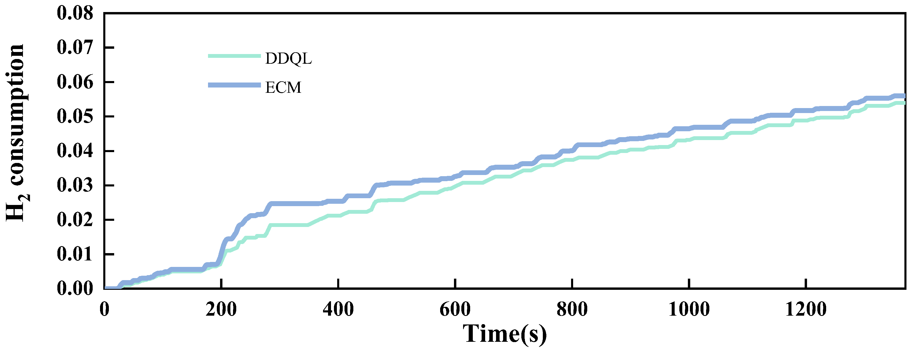
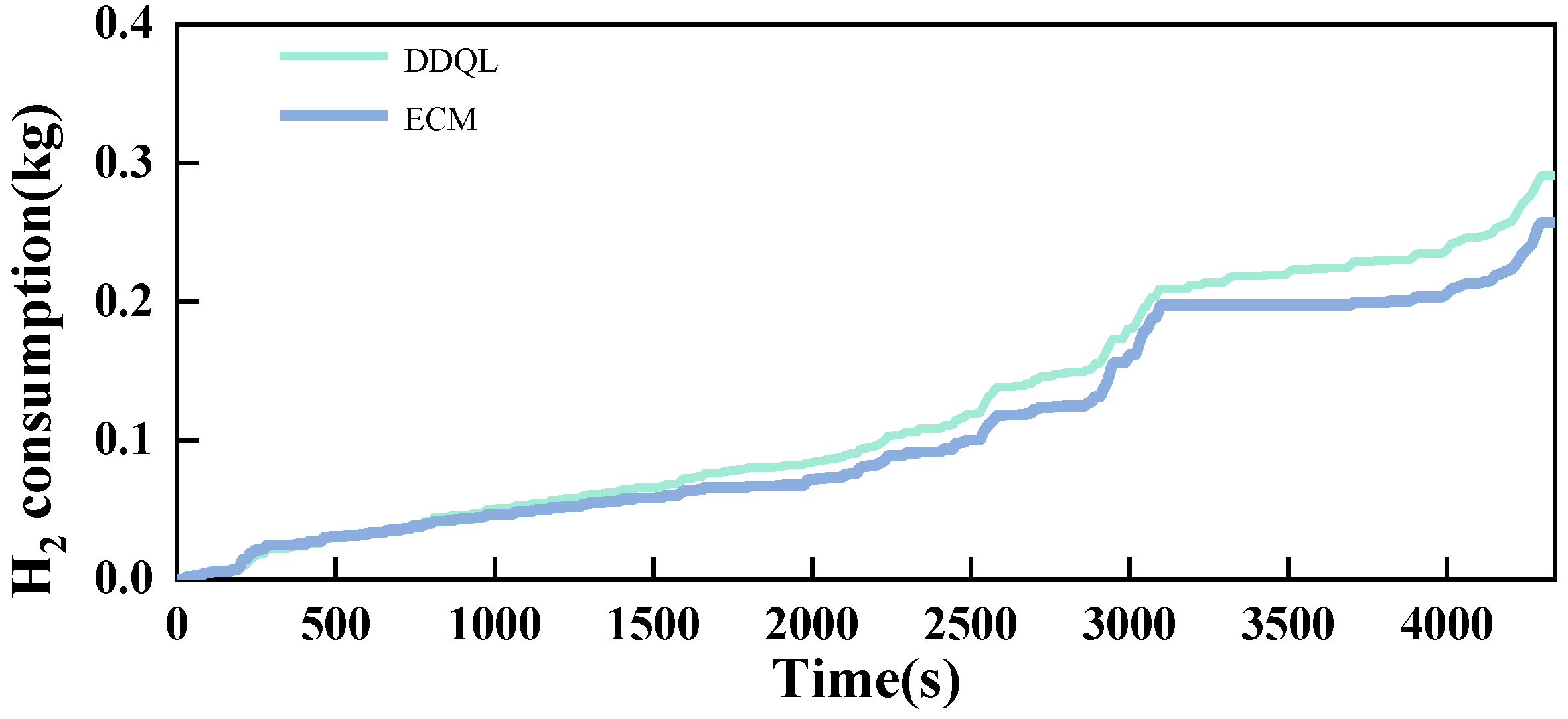
Figure 9 depicts the power distribution of ECM-based EMS under the UDDS cycle. Figure 9a shows the power distribution performance of the ECM-based EMS. From 150 to 300 s, the power demand of vehicle exhibited sharp fluctuations, with fuel cell peak output power exceeding 30 kW and significant power fluctuations between adjacent moments. In order to maintain consistency between the initial and final SOC states of LIB, fuel cells underwent drastic changes in demand power throughout the entire cycle.

On the contrary, the FCS power of DDQL-based EMS was maintained within 10 kW throughout the entire cycle, as shown in Figure 9b. Especially in the frequent variable load range from 150 to 300 s, FCS maintained high-efficiency output power around 20 kW, and the peak power was supplemented by LIB.

Based on the power distribution described above, the output efficiency of the FCS at each moment can be determined, as illustrated in Figure 10a. The efficiency of ECM-based EMS exhibited sharp fluctuation with a mean efficiency 58.59%. This occurred because it consistently fluctuated with the overall demand, prolonging the operating duration of FCS under condition of high power and low efficiency. On the contrary, the proposed strategy ensured that the FCS operated consistently within a high-efficiency range with mean efficiency 62.51%. Although the overall operating duration of FCS increased, the working time at the high-efficiency point also increased. This resulted in a 4% increase in the FCS output efficiency and a decrease in fuel consumption after completing the cycle, ultimately leading to a reduction in overall hydrogen consumption, as shown in Figure 10b,c.

4.3.2. Fuel Economy

The amount of hydrogen consumed at each second can be calculated by power, as depicted in Figure 11. From 0 to 300 s, there was an increase in power demand, leading to an increase in the output of the FCS by ECM, consequently escalating the rate of hydrogen consumption. Simultaneously, the DDQL-based EMS was adjusted to slightly enhance the output of FCS, while the remainder was supplemented by LIB. This approach minimized the operating duration at high-power and low-efficiency points, enhanced overall efficiency, and diminished hydrogen consumption over the entire cycle.

The results indicate that under UDDS operating conditions, the ECM-based EMS consumed 466.7 g/100 km of hydrogen, whereas the DDQL-based EMS consumed 449.1 g/100 km of hydrogen. Therefore, compare to ECM-based EMS, the proposed DDQL-based EMS has better fuel economy.

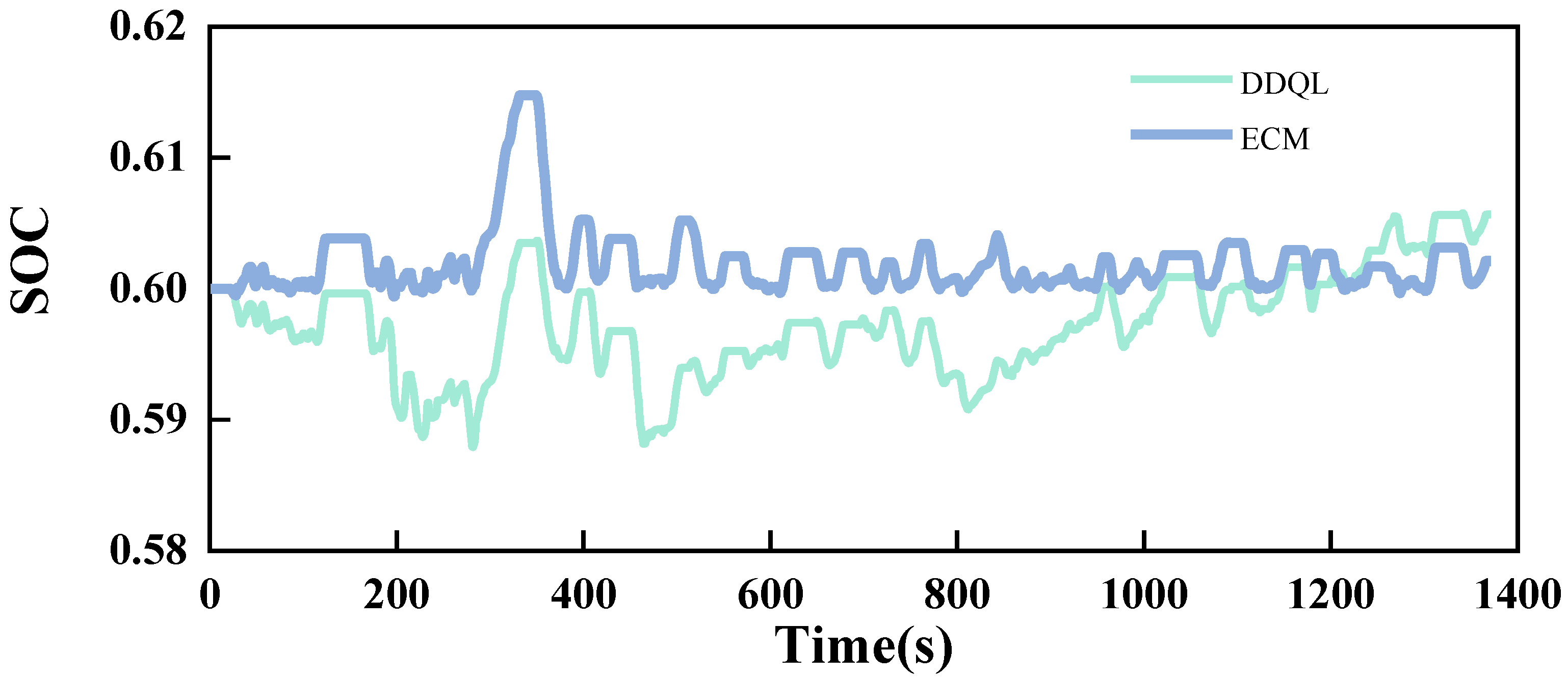
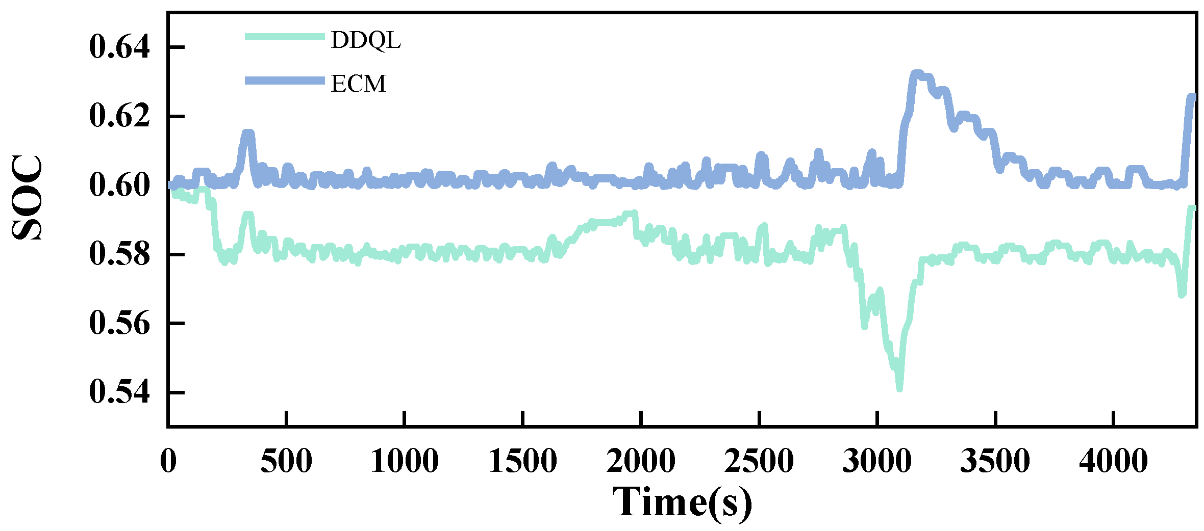
4.3.3. SOC Consistency

Figure 12 depicts the SOC trajectory of the ECM- and DDQL-based EMSs. It clearly shows that the SOC curve changed within the operational interval (0.4–0.9). The DDQL-based EMS maintained fluctuations between 0.58 and 0.6, while the ECM-based EMS maintained the SOC range within 0.6–0.62. The main reason is that ECM-based EMS primarily consumed the output power of the fuel cell, and LIB primarily served as a supplement, resulting in smaller decrease in the SOC, and the SOC in the final state was at 0.602, while the DDQL-based EMS’s final state SOC remained at 0.605.

This result indicates that both strategies can maintain the SOC stability. Also, the fluctuation range of DDQL-based EMS was wider than ECM-based EMS. This was mainly due to the fact that ECM-based EMS increased the output power of FCS to adapt to frequent changes in demand power and peak output, while LIB had fewer outputs and smoother output fluctuations. Especially in the 200 to 600 s, the fluctuation of DDQL-based EMS was larger than ECM-based EMS.

Therefore, compare to the ECM-based EMS, the proposed DDQL-based EMS can maintain the SOC consistency by allocating the power distribution properly.

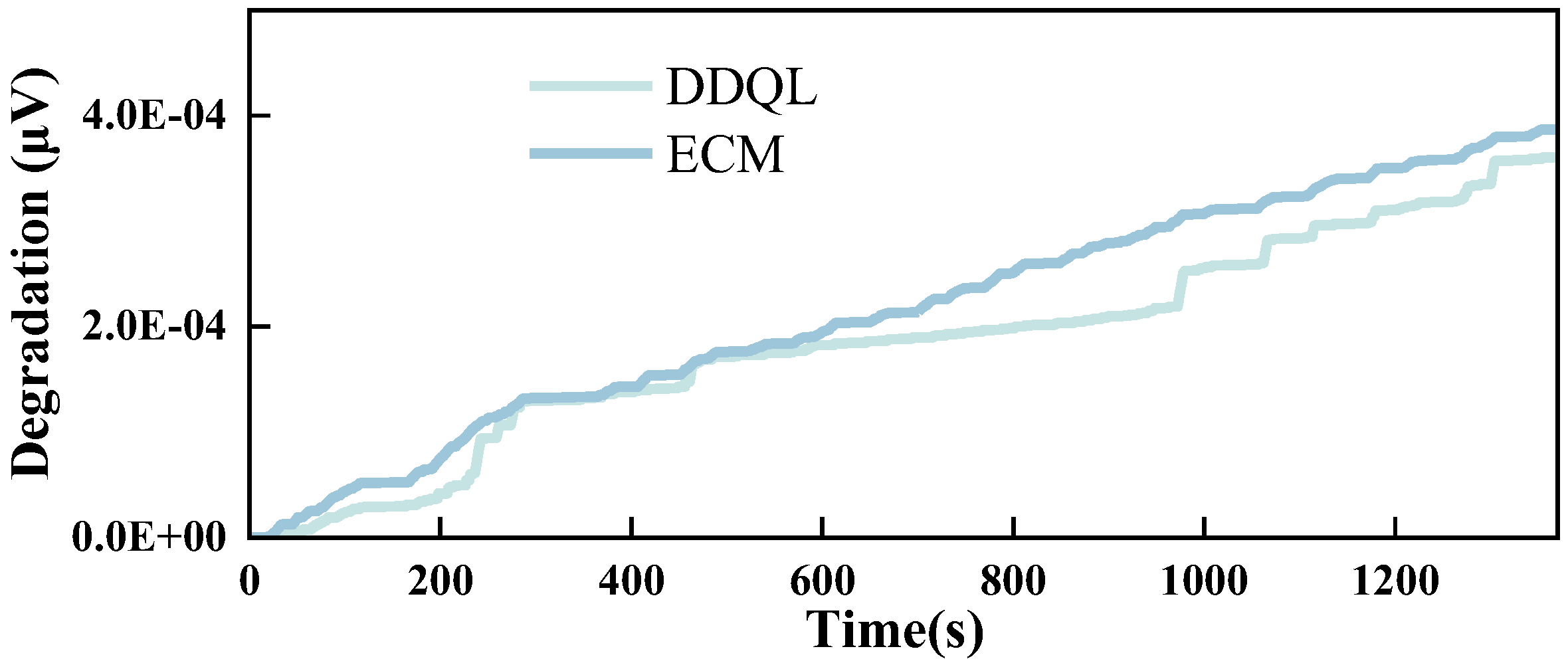
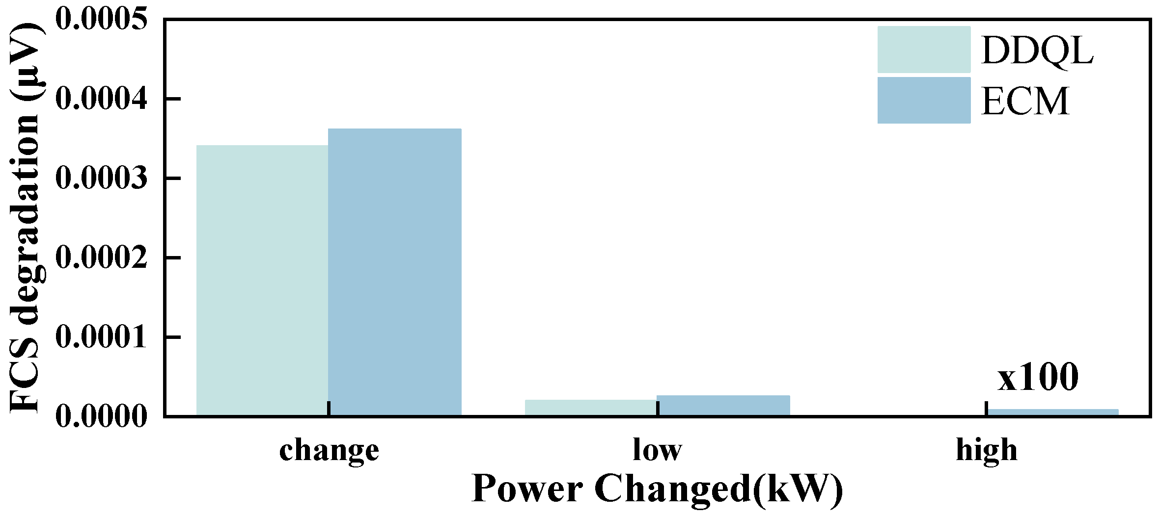
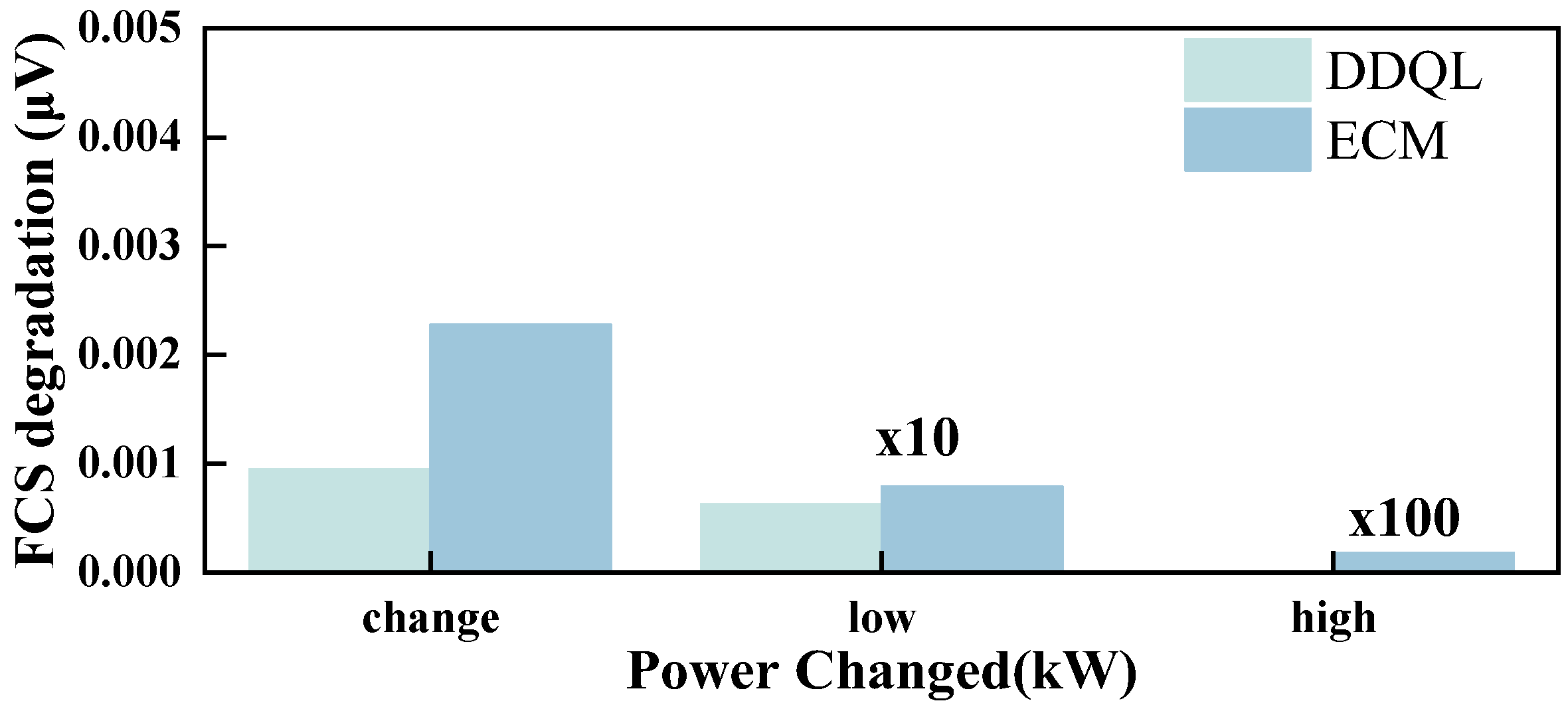
4.3.4. FCS Degradation

In the above subsection, the effectiveness of the proposed strategy in achieving better fuel economy is demonstrated. However, the durability of the FCS has not been verified. Therefore, in the following section, this paper analyzes the proposed strategy from the perspective of fuel cell durability and adds the FCS performance decay rate as an indicator. The reward function of DDQL-based EMS is calculated.

Figure 13 illustrates the trajectories of FCS performance degradation for the two strategies under the UDDS cycle. The ECM-based EMS was attenuated by 0.00036 μV, while DDQL-base EMS was attenuated by 0.0003872 μV. This is primarily attributed to the continuous adjustment of FCS under the UDDS cycle. The output power fluctuated to meet the required power as the working conditions changed, resulting in an elevation of the FCS operating point under variable load conditions, thereby exacerbating the impact of variable load conditions on the performance degradation of the FCS. Furthermore, the energy management strategy based on DDQL also reduced the operating points at high power and low power, mitigating the impact of these operating conditions on fuel cell performance, as shown in Figure 14.

4.4. The Feasibility of Both Strategies in Different Environments

To further investigate the performance of DDQL-based EMS in terms of fuel economy and battery charge sustainability, this paper compares the performance of ECM-based EMS and DDQL-based EMS under the combined cycle, as shown in Figure 7b. The initial SOC value was set to 0.6.

Figure 15, Figure 16, Figure 17, Figure 18 and Figure 19 depict each indicator of the EMS. The results indicate that under the combined cycle, the DDQL-based EMS optimally allocated the output power of FCS within the high-efficiency range. It employed LIB as auxiliary energy to diminish the operational duration of FCS at low-efficient operating points during frequent load variations. By mitigating the frequent load fluctuations of fuel cells, as illustrated in Figure 19, the adverse impact of various operating points on the voltage degradation of the FCS was minimized, thus prolonging its service life, as shown in Figure 18.

Figure 16 illustrates the hydrogen consumption throughout the entire cycle under the combined cycle. In comparison to the ECM-based EMS, the DDQL-based EMS exhibited a slight increase in hydrogen consumption. This is primarily attributed to the fact that during 3200–3800 s, the FCS power output from the ECM-based EMS was zero, with the main output sourced from LIB. The energy consumed by LIB was derived from the recovered braking energy between 2800 and 3200 s, leading to a marginally lower overall hydrogen consumption compared to DDQL-based EMS.

Meanwhile, although the output of LIB under the DDQL-based EMS fluctuated greatly during operation, their SOC was still in the high-efficiency and safe range of 0.4–0.8, and the final state SOC was 0.594, which could be well maintained around 0.6. The ECM-based EMS yielded a final SOC of 0.624, as shown in Figure 17. This is primarily attributed to the fluctuation of FCS output in response to the load variation throughout the entire cycle, while the consumption of LIB remained minimal. Consequently, there was a significant increase in SOC due to the greater energy recovery toward the end of the NEDC cycle. Compared with the initial state of 0.6, the energy management strategy based on DDQL can better maintain the consistency of SOC initial and final states.

Table 5. Comparison of hydrogen consumption and life degradation.

Cycle	DDQL			ECM
	H2 Consumption g/100 km	SOC	FCS Degradation μV	H2 Consumption g/100 km	SOC	FCS Degradation μV
UDDS	449.1	0.605	0.00036	466.7	0.602	0.0003872
Combined	627.3 g	0.594	0.001031	555.5	0.624	0.002339

compares the DDQL-based EMS to ECM-based EMS in terms of hydrogen consumption, SOC consistency, and FCS degradation under various driving cycle.

5. Conclusions

This paper presents a reinforcement learning-based energy management strategy considering fuel cell voltage degradation. The primary aim of this strategy is to reduce fuel cell voltage performance degradation, prolonging the service life of fuel cells, while ensuring the safe and stable operation of lithium batteries and maintaining consistency between their initial and final states. With these objectives in mind, a framework for energy strategy management based on deep reinforcement learning was devised according to the FCEV model, and the strategy was optimized using the DDQL algorithm. The DDQL-based EMS was trained under UDDS and tested under combined UDDS-WLTC-NEDC operating conditions. To validate the effectiveness of the proposed strategy, ECM-based EMS was used as a benchmark for comparison. The results indicate that under training conditions, the DDQL-based strategy can reduce fuel consumption while effectively maintaining the consistency of SOC between initial and final states, thereby extending the service life of fuel cells. Under verification conditions, the DDQL-based energy management strategy effectively preserved the consistency of SOC between initial and final states and reduced voltage degradation by 50% through a slight increase in fuel consumption, thereby increasing the service cycle.

In practical applications, both state variables and control variables are continuous signals. While DDQL-based EMS can handle the dimensional signals, it is challenging to output the continuous signals. Therefore, exploring intelligent RL agent capable of output continuous actions is necessary for the future research.

References

1. Sorlei, I.-S.; Bizon, N.; Thounthong, P.; Varlam, M.; Carcadea, E.; Culcer, M.; Iliescu, M.; Raceanu, M. Fuel Cell Electric Vehicles—A Brief Review of Current Topologies and Energy Management Strategies. Energies 2021, 14, 252. [Google Scholar] [CrossRef]
2. Ma, S.; Lin, M.; Lin, T.-E.; Lan, T.; Liao, X.; Maréchal, F.; Van herle, J.; Yang, Y.; Dong, C.; Wang, L. Fuel Cell-Battery Hybrid Systems for Mobility and off-Grid Applications: A Review. Renew. Sustain. Energy Rev. 2021, 135, 110119. [Google Scholar] [CrossRef]
3. Han, J.; Feng, J.; Chen, P.; Liu, Y.; Peng, X. A Review of Key Components of Hydrogen Recirculation Subsystem for Fuel Cell Vehicles. Energy Convers. Manag. X 2022, 15, 100265. [Google Scholar] [CrossRef]
4. Hua, Z.; Zheng, Z.; Pahon, E.; Péra, M.-C.; Gao, F. A Review on Lifetime Prediction of Proton Exchange Membrane Fuel Cells System. J. Power Sources 2022, 529, 231256. [Google Scholar] [CrossRef]
5. Miotti, M.; Hofer, J.; Bauer, C. Integrated Environmental and Economic Assessment of Current and Future Fuel Cell Vehicles. Int. J. Life Cycle Assess 2017, 22, 94–110. [Google Scholar] [CrossRef]
6. Zhang, Y.; Zhang, C.; Fan, R.; Huang, S.; Yang, Y.; Xu, Q. Twin Delayed Deep Deterministic Policy Gradient-Based Deep Reinforcement Learning for Energy Management of Fuel Cell Vehicle Integrating Durability Information of Powertrain. Energy Convers. Manag. 2022, 274, 116454. [Google Scholar] [CrossRef]
7. Luo, M.; Zhang, J.; Zhang, C.; Chin, C.S.; Ran, H.; Fan, M.; Du, K.; Shuai, Q. Cold Start Investigation of Fuel Cell Vehicles with Coolant Preheating Strategy. Appl. Therm. Eng. 2022, 201, 117816. [Google Scholar] [CrossRef]
8. Krithika, V.; Subramani, C. A Comprehensive Review on Choice of Hybrid Vehicles and Power Converters, Control Strategies for Hybrid Electric Vehicles. Int. J. Energy Res. 2018, 42, 1789–1812. [Google Scholar] [CrossRef]
9. Liu, S.; Du, C.; Yan, F.; Wang, J.; Li, Z.; Luo, Y. A Rule-Based Energy Management Strategy for a New BSG Hybrid Electric Vehicle. In Proceedings of the 2012 Third Global Congress on Intelligent Systems, Wuhan, China, 6–8 November 2012; IEEE: Piscataway, NJ, USA, 2012; pp. 209–212. [Google Scholar]
10. Peng, H.; Li, J.; Thul, A.; Deng, K.; Ünlübayir, C.; Löwenstein, L.; Hameyer, K. A Scalable, Causal, Adaptive Rule-Based Energy Management for Fuel Cell Hybrid Railway Vehicles Learned from Results of Dynamic Programming. eTransportation 2020, 4, 100057. [Google Scholar] [CrossRef]
11. Liu, C.; Wang, Y.; Wang, L.; Chen, Z. Load-Adaptive Real-Time Energy Management Strategy for Battery/Ultracapacitor Hybrid Energy Storage System Using Dynamic Programming Optimization. J. Power Sources 2019, 438, 227024. [Google Scholar] [CrossRef]
12. Peng, H.; Chen, Z.; Li, J.; Deng, K.; Dirkes, S.; Gottschalk, J.; Ünlübayir, C.; Thul, A.; Löwenstein, L.; Pischinger, S. Offline Optimal Energy Management Strategies Considering High Dynamics in Batteries and Constraints on Fuel Cell System Power Rate: From Analytical Derivation to Validation on Test Bench. Appl. Energy 2021, 282, 116152. [Google Scholar] [CrossRef]
13. Musardo, C.; Rizzoni, G.; Guezennec, Y.; Staccia, B. A-ECMS: An Adaptive Algorithm for Hybrid Electric Vehicle Energy Management. Eur. J. Control 2005, 11, 509–524. [Google Scholar] [CrossRef]
14. Huang, Y.; Wang, H.; Khajepour, A.; He, H.; Ji, J. Model Predictive Control Power Management Strategies for HEVs: A Review. J. Power Sources 2017, 341, 91–106. [Google Scholar] [CrossRef]
15. Xie, S.; Hu, X.; Qi, S.; Tang, X.; Lang, K.; Xin, Z.; Brighton, J. Model Predictive Energy Management for Plug-in Hybrid Electric Vehicles Considering Optimal Battery Depth of Discharge. Energy 2019, 173, 667–678. [Google Scholar] [CrossRef]
16. Zheng, Y.; He, F.; Shen, X.; Jiang, X. Energy Control Strategy of Fuel Cell Hybrid Electric Vehicle Based on Working Conditions Identification by Least Square Support Vector Machine. Energies 2020, 13, 426. [Google Scholar] [CrossRef]
17. Zhou, Y.; Ravey, A.; Péra, M.-C. Multi-Mode Predictive Energy Management for Fuel Cell Hybrid Electric Vehicles Using Markov Driving Pattern Recognizer. Appl. Energy 2020, 258, 114057. [Google Scholar] [CrossRef]
18. Reddy, N.P.; Pasdeloup, D.; Zadeh, M.K.; Skjetne, R. An Intelligent Power and Energy Management System for Fuel Cell/Battery Hybrid Electric Vehicle Using Reinforcement Learning. In Proceedings of the 2019 IEEE Transportation Electrification Conference and Expo (ITEC), Detroit, MI, USA, 19–21 June 2019; IEEE: Piscataway, NJ, USA, 2019; pp. 1–6. [Google Scholar]
19. Sun, W.; Qiu, Y.; Sun, L.; Hua, Q. Neural Network--based Learning and Estimation of Battery state--of--charge: A Comparison Study between Direct and Indirect Methodology. Int. J. Energy Res. 2020, 44, 10307–10319. [Google Scholar] [CrossRef]
20. Sun, L.; Wang, X.; Su, Z.; Hua, Q.; Lee, K.Y. Energy Management of a Fuel Cell Based Residential Cogeneration System Using Stochastic Dynamic Programming. Process Saf. Environ. Prot. 2023, 175, 272–279. [Google Scholar] [CrossRef]
21. Li, W.; Cui, H.; Nemeth, T.; Jansen, J.; Uenluebayir, C.; Wei, Z.; Zhang, L.; Wang, Z.; Ruan, J.; Dai, H. Deep Reinforcement Learning-Based Energy Management of Hybrid Battery Systems in Electric Vehicles. J. Energy Storage 2021, 36, 102355. [Google Scholar] [CrossRef]
22. Wang, Y.; Moura, S.J.; Advani, S.G.; Prasad, A.K. Power Management System for a Fuel Cell/Battery Hybrid Vehicle Incorporating Fuel Cell and Battery Degradation. Int. J. Hydrogen Energy 2019, 44, 8479–8492. [Google Scholar] [CrossRef]
23. Song, K.; Ding, Y.; Hu, X.; Xu, H.; Wang, Y.; Cao, J. Degradation Adaptive Energy Management Strategy Using Fuel Cell State-of-Health for Fuel Economy Improvement of Hybrid Electric Vehicle. Appl. Energy 2021, 285, 116413. [Google Scholar] [CrossRef]
24. Sun, H.; Fu, Z.; Tao, F.; Zhu, L.; Si, P. Data-Driven Reinforcement-Learning-Based Hierarchical Energy Management Strategy for Fuel Cell/Battery/Ultracapacitor Hybrid Electric Vehicles. J. Power Sources 2020, 455, 227964. [Google Scholar] [CrossRef]
25. Zhang, Z.; Guan, C.; Liu, Z. Real-Time Optimization Energy Management Strategy for Fuel Cell Hybrid Ships Considering Power Sources Degradation. IEEE Access 2020, 8, 87046–87059. [Google Scholar] [CrossRef]
26. Mann, R.F.; Amphlett, J.C.; Hooper, M.A.; Jensen, H.M.; Peppley, B.A.; Roberge, P.R. Development and Application of a Generalised Steady-State Electrochemical Model for a PEM Fuel Cell. J. Power Sources 2000, 86, 173–180. [Google Scholar] [CrossRef]
27. Pei, P.; Chang, Q.; Tang, T. A Quick Evaluating Method for Automotive Fuel Cell Lifetime. Int. J. Hydrogen Energy 2008, 33, 3829–3836. [Google Scholar] [CrossRef]
28. Johnson, V.H. Battery Performance Models in ADVISOR. J. Power Sources 2002, 110, 321–329. [Google Scholar] [CrossRef]
Figure 1. The structural schematic diagram of the FCEV.
Energies 17 01586 g001
Figure 2. The mechanism of the fuel cell.
Energies 17 01586 g002
Figure 3. The relationship between total power of FCS and the efficiency.
Energies 17 01586 g003
Figure 4. The diagram of a lithium-ion battery [28].
Energies 17 01586 g004
Figure 5. The relationship between the open-circuit voltage and SOC.
Energies 17 01586 g005
Figure 6. Energy management strategy framework based on the DDQL algorithm.
Energies 17 01586 g006
Figure 7. Speed curve of (a) UDDS cycle; (b) combined cycle.
Energies 17 01586 g007
Figure 8. The reward comparison of both strategies.
Energies 17 01586 g008
Figure 9. The power distribution of two strategies: (a) ECM-EMS, (b) DDQL-EMS.
Energies 17 01586 g009
Figure 10. (a) the efficiency of two strategies in UDDS (b) the efficiency distribution of two strategies, (c) the power distribution of two strategies.
Energies 17 01586 g010
Figure 11. The H2 consumption of FCS.
Energies 17 01586 g011
Figure 12. The SOC trajectory of both strategies.
Energies 17 01586 g012
Figure 13. Comparison FCS degradation for different strategies.
Energies 17 01586 g013
Figure 14. The degradation distribution of two strategies.
Energies 17 01586 g014
Figure 15. The power allocation of both strategies in the combined cycle: (a) ECM-based EMS (b) DDQL-based EMS.
Energies 17 01586 g015
Figure 16. The fuel consumption trajectory of both strategies in the combined cycle.
Energies 17 01586 g016
Figure 17. The SOC trajectory of both strategies in the combined cycle.
Energies 17 01586 g017
Figure 18. The FCS degradation trajectory of both strategies in the combined cycle.
Energies 17 01586 g018
Figure 19. The FCS degradation distribution under the different operation conditions.
Energies 17 01586 g019