Active Disturbance Rejection Control Design with Sensitivity Constraint for Drum Water Level

Abstract

The drum water level plays a crucial role in the safety and economy of heat recovery boilers. However, the control of the drum water level faces many challenges, such as external disturbances and system uncertainties. To enhance the control performance of the drum water level, a modified active disturbance rejection control (MADRC) optimized with sensitivity constraint is proposed in this paper. Firstly, the control structure of the three-element control system for the drum water level is introduced and analyzed. Based on the regular active disturbance rejection control (ADRC) structure, the structure of the MADRC is introduced and the convergence of the proposed MADRC is proven. Then a modified whale optimization algorithm (MWOA) with sensitivity constraint is applied to optimize the parameters of the MADRC. With different sensitivity constraints, the parameters of the MADRC and comparative controllers are obtained, and their control performance for tracking and disturbance rejection abilities is compared. Moreover, the ability to handle system uncertainties is analyzed. Simulation results and performance indexes show that the proposed MADRC can obtain the best tracking and disturbance rejection abilities with satisfactory robustness. The satisfactory control performance shows that the proposed MADRC has wide application potential for heat recovery boilers and other industrial processes.

1. Introduction

With more and more renewable energy sources, such as wind power and photovoltaics, integrating into the power grid, heat recovery boilers combing gas turbines with fast load response speed and environmental friendliness are playing crucial roles for the stability and safety of the power grid [1]. However, the drum water level, as the most important subsystem, is facing many challenges caused by fluctuations of the steam flow and feed water flow [2].

To improve the stability of the drum water level, the drum water level control plays the most important role, considering that the drum water level faces many external disturbances and system uncertainties [3]. To enhance the control performance of the drum water level for heat recovery boilers, different control strategies have been studied and designed. The classical proportional-integral-derivative (PID) controllers, with a simple structure and reliable control performance, have been designed widely for the drum water level [4,5]. Modified PID controllers, such as the adaptive PID controller [6] and fuzzy PID controller [7], also have been optimized to enhance the ability of a PID to handle system nonlinearity of the drum water level. However, the implementation difficulties of modified PID controllers are the main limitations of their extensive applications [8]. In addition, the fractional-order PID (FOPID) controller, as the generalization of a PID controller, with the advantage of more freedom degrees for parameter tuning, is also being tried to apply to the drum water level of heat recovery boilers [9,10]. Note that the FOPID controller is facing implementation difficulties, where the FOPID is approximated by high-order integer order transfer functions in a distributed control system (DCS). Simulation results have illustrated the improvement of the control performance of the drum water level, while rare on-site applications have been reported. A robust controller, with a small dependency on the accurate mathematical model, is also applied to the drum water level [11,12], where the worst-case condition is also considered in the process of controller design [13]. The relatively conservative control performance makes the robust controller highly adaptable to model uncertainties [14]. However, the relatively conservative control performance is the main shortcoming. A sliding mode controller has strong robustness against the variation of system parameters and disturbances, but at the same time, variable structure control technology also has a serious drawback: the jitter of the control signal. This would cause irreversible wear of the actuator and have a significant impact on the economic operation of the drum water level system [15,16]. With advantages in handling multivariable coupling and system nonlinearity, the model predictive control (MPC) controller is also structured for the drum water level system and satisfactory control performance can be obtained under the nominal operating condition [17,18]. Unfortunately, the control performance would seriously decline if operating conditions work far from the nominal operating condition. With the development of computer hardware and artificial intelligence technology, complex control algorithms, such as fuzzy controller [19], neural network controller [20] and reinforcement learning controller [21], are also proposed for the drum water level. Although satisfactory control performance can be achieved, theoretical convergence proof of these controllers is lacking.

Considering that the drum water level faces many challenges, such as external disturbances and system uncertainties, the suitable controller of the drum water level should have the following features: strong robustness, weak independence of the accurate mathematical model and strong ability to reject multi-source disturbances [22]. The active disturbance rejection control (ADRC), with the features mentioned above, is receiving more and more attention. With the online estimation and real-time compensation disturbances by extended state observer (ESO), the ADRC can track the set point and reject disturbances well. With the strong ability of ESO to estimate and compensate for the total disturbance, the ADRC has strong robustness to handle system uncertainties [23]. With comprehensive theoretical analysis and rich parameter tuning methods [24], the excellent control performance has been verified in different applications, such as applications in robotic systems [25], main steam pressure systems [26], superheater temperature systems [27], particleboard glue systems [28], aircraft anti-skid braking systems [29] and compression liquid chiller systems [30].

In fact, the ADRC also has been tried to apply to the drum water level for heat recovery boilers [31,32,33]. Considering the limitations on the upper limit of the observer bandwidth of ESO, the control performance of the drum water level is limited, and this paper proposes a modified ADRC (MADRC) to increase the upper limit of observer bandwidth inspired by Ref. [27]. Moreover, how to select the reasonable parameters of the ADRC also is a non-negligible problem. To tune the appropriate controller parameters, a modified whale optimization algorithm (MWOA) [34] with sensitivity constraint is applied to optimize the parameters of the MADRC, where the maximum sensitivity function is applied to guarantee that the controller has the specified robustness. The main contributions of this paper are summarized as follows:

(1)

An MADRC is proposed, and the convergence of the proposed MADRC is proven;

(2)

An MWOA with sensitivity constraint is applied to optimize the parameters of the MADRC, where the bandwidths of the controller and ESO can be selected with sensitivity constraint;

(3)

The effectiveness of the proposed MADRC optimized by the MWOA is verified by comparative simulations.

The rest of this paper is arranged as follows: The structure of the drum water level is introduced in Section 2. The introductions of the regular ADRC and MADRC are presented in Section 3. In addition, the convergence analysis of the MADRC is also carried out. The MWOA is applied to optimize the parameters of the MADRC, where the maximum sensitivity function is used as the robustness constraint in Section 4. Section 5 presents the comparative simulation results in the nominal condition with different sensitivity constraints and uncertain conditions. Section 6 provides some conclusions of the paper.

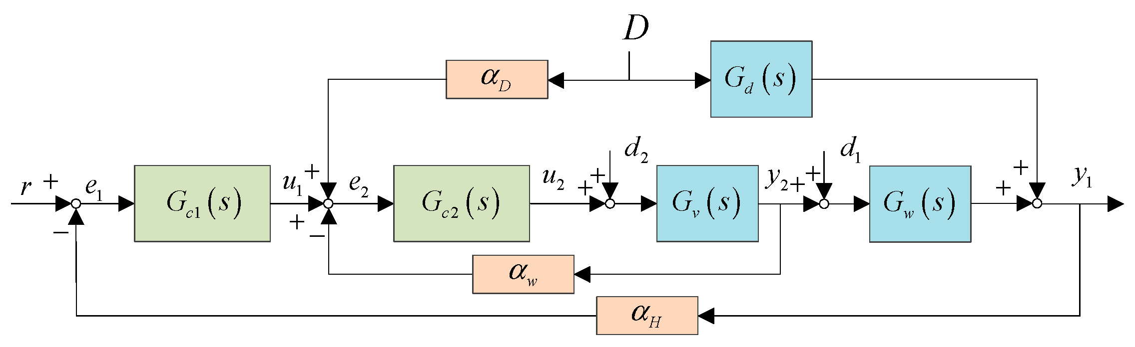
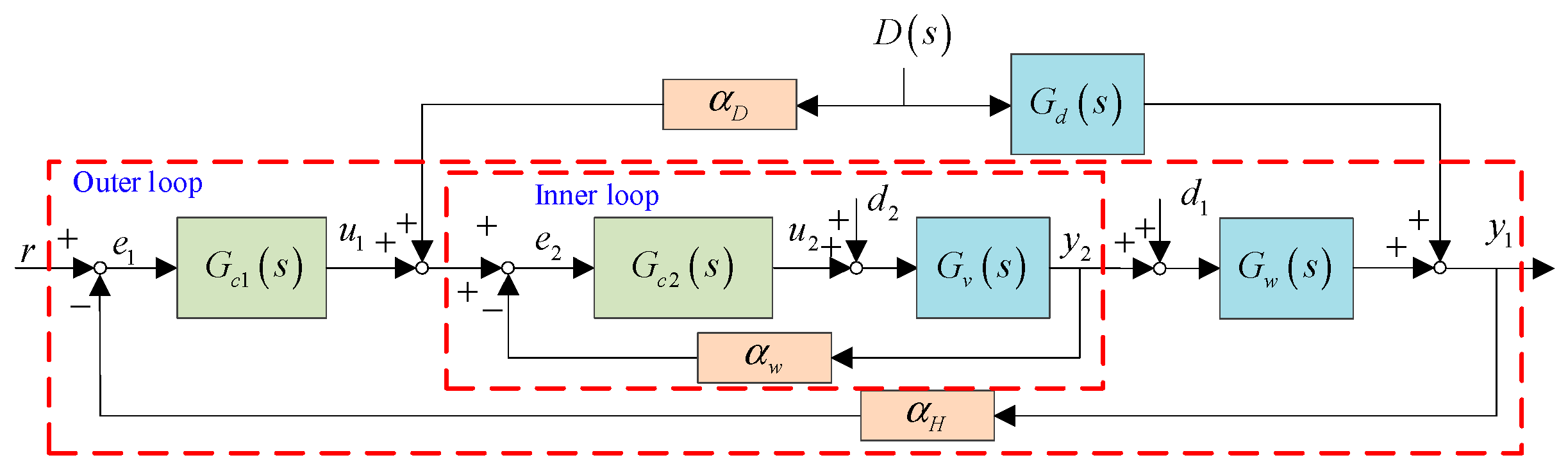
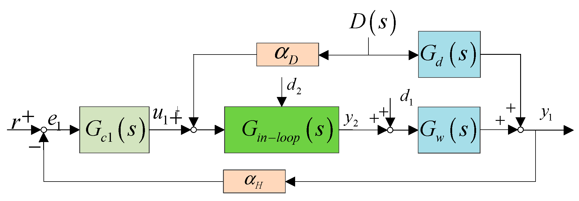
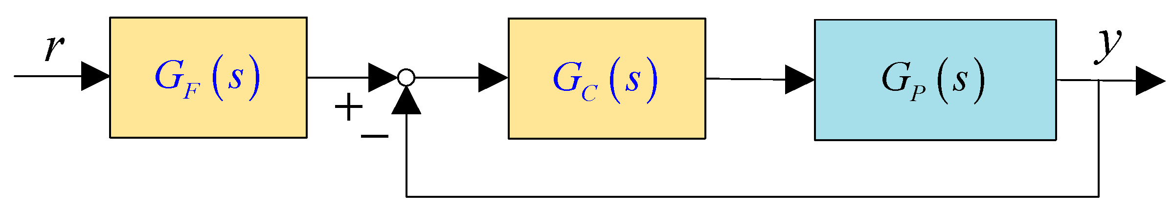
2. Control Structure of Drum Water Level and Control Objective

The operational quality of the drum water level is significant for the safety of the water circulation. The steam would carry water if the drum water level is too high. Similarly, the boiler would dry out if the drum water level is too low. Therefore, the drum water level should be controlled in a reasonable range. Strong abilities to track and disturbance rejection are critical factors for the high-quality operation of the drum water level. The classical and universal control structure of the drum water level is called the three-element system, where the control structure contains a cascade structure and a feedforward controller as presented in Figure 1. $r$, $y_1$ and $y_2$ are the set point of $y_1$, the drum water level and the feed water flow, respectively. $d_1$ and $d_2$ are the external disturbance (measurement error of drum water level etc.) and inner disturbance (steam flow disturbance etc.), respectively. $D$ is the steam flow.

The dynamic process from $y_2$ to $y_1$ is depicted by

$${\dot{y}}_1+30{\ddot{y}}_1-0.037y_2=0.$$

(1)

The dynamic process from the valve opening $u_2$ to $y_2$ is depicted by

$$5{\dot{y}}_2+y_2-20u_2=0.$$

(2)

The dynamic process from $D$ to $y_1$ is depicted by

$${\dot{y}}_1+15{\ddot{y}}_1-3.045{\dot{D}}_2+0.037D_2=0.$$

(3)

Equations (1)–(3) can be equivalent to the following transfer functions ($G_w\left(s\right)$, $G_v\left(s\right)$ and $G_d\left(s\right)$) as

$$G_w\left(s\right)=\frac{0.037}{(30s+1)s},$$

(4)

$$G_v\left(s\right)=\frac{20}{5s+1},$$

(5)

and

$$G_d\left(s\right)=\frac{3.6}{15s+1}-\frac{0.037}{s}.$$

(6)

In addition, $G_{c1}\left(s\right)$ and $G_{c2}\left(s\right)$ are the master controller and slave controller, respectively. ${\alpha }_D=0.0174$, ${\alpha }_w=0.0174$ and ${\alpha }_H=1$ are the transmission coefficients of $D\left(s\right)$, $y_2$ and $y_1$, respectively.

To ensure the high-quality operation of the drum water level, the parameters of $G_{c1}\left(s\right)$ and $G_{c2}\left(s\right)$ should be tuned reasonably and optimally. Considering that the inner loop has the fast dynamic characteristic, the PID controller can be selected as $G_{c1}\left(s\right)=k_{p1}+k_{i1}/s+k_{d1}s$.

The closed-loop of the inner loop as presented in Figure 2 can be obtained as

$$G_{in-loop}\left(s\right)=\frac{G_{c2}\left(s\right)G_v\left(s\right)}{1+G_{c2}\left(s\right)G_v\left(s\right){\alpha }_w}.$$

(7)

Then, the transfer function for the outer loop from $r$ to $y_1$ can be obtained as,

$$Y_1\left(s\right)=G_w\left(s\right)D_1\left(s\right)+G_d\left(s\right)D\left(s\right)+Y_2(s)G_w\left(s\right),$$

(8)

where

$$Y_2(s)=Y_{u_1}(s)+Y_{d_2}(s)+Y_D(s),$$

(9)

$$Y_{u_1}(s)=G_{in-loop}\left(s\right)\left(R\left(s\right)-{\alpha }_{H}Y\left(s\right)\right)G_{c1}\left(s\right),$$

(10)

$$Y_{d_2}(s)=\frac{G_{in-loop}\left(s\right)}{G_{c2}\left(s\right)}{D}_2\left(s\right),$$

(11)

$$Y_D(s)={\alpha }_D{G}_{in-loop}\left(s\right)D_2\left(s\right).$$

(12)

With the equivalent structure in Figure 3, the definition of $G_{in-loop}\left(s\right)$ and the PID of $G_{c1}\left(s\right)$, one can have the outer controlled plant as

$$G_{out-loop}(s)=G_{in-loop}\left(s\right)G_w\left(s\right)=\frac{Y_1\left(s\right)}{U_1\left(s\right)}.$$

(13)

Further,

$$G_{out-loop}(s)=\frac{0.74\left(k_{d1}{s}^2+k_{p1}s+k_{i1}\right)}{s\left(30s+1\right)\left[\left(0.348k_{d1}+5\right)s^2+\left(0.348k_{p1}+1\right)s+0.348k_{i1}\right]}.$$

(14)

To enhance the control performance of the drum water level in Figure 1, a second-order ADRC, as the master controller, can be designed for this system, considering that the relative order of $G_{out-loop}(s)$ is 2. With tuned $G_{c1}\left(s\right)$, one can have $G_{in-loop}\left(s\right)\approx 1$ as discussed in Ref. [27], and Equation (13) can be approximated as

$$G_{out-loop}(s)\approx \frac{1}{s\left(30s+1\right)}.$$

(15)

Moreover, the control signal of $u_2$ is recommended as $\left[-20,20\right]$ to protect the feed pump.

The control objective of the control structure of the drum water level can be listed as follows:

• $y_1$ tracks $r$ as fast as possible with small overshoot;
• The closed-loop system can quickly recover to the steady state when $D\left(s\right)$, $d_1$ or $d_2$ occurs;
• The closed-loop system should have a strong ability to handle system uncertainties.

To guarantee the robustness of the ADRC, i.e., the ability to handle system uncertainties, the maximum sensitivity function, a widely used indicator for controllers [35], is selected as the robustness measurement indicator. The definition of robustness constraint, the maximum sensitivity value of the maximum sensitivity function, i.e., $M_s$, can be depicted as

$$M_s=\underset{0\le \omega <\infty }{\max }\left|\frac{1}{1+{\alpha }_H{G}_{c1}\left(j\omega \right)G_{in-loop}\left(j\omega \right)}\right|,$$

(16)

where $M_s$ can be regarded as the reciprocal of the nearest distance from the Nyquist curve of the open-loop system to $\left(-1,0j\right)$ as presented in Figure 4, i.e., the reciprocal of the distance from point A to the $\left(-1,0j\right)$. The recommended range of $M_s$ is [1.2~2.0], where a larger $M_s$ means weaker robustness and vice versa [36].

The objective to optimize parameters of $G_{c1}\left(s\right)$ can be depicted by

$$\begin{gathered} \mathrm{Min} \mathrm{control} \mathrm{performance} \mathrm{of} G_{out-closedloop}\left(s\right) \mathrm{with} \mathrm{respect} \mathrm{to} \mathit{x} \\ \mathrm{Subject} \mathrm{to}: M_s\in \left[q_{-},q_{+}\right] \end{gathered}$$

(17)

where the control performance of the closed-loop $G_{out-closedloop}\left(s\right)=\frac{G_{c1}\left(s\right)G_{in-loop}\left(s\right)}{1+{\alpha }_H{G}_{c1}\left(s\right)G_{in-loop}\left(s\right)}$ can be defined as the integral of absolute error (IAE), the integral of time absolute error (ITAE), the integral of error (IE), etc.

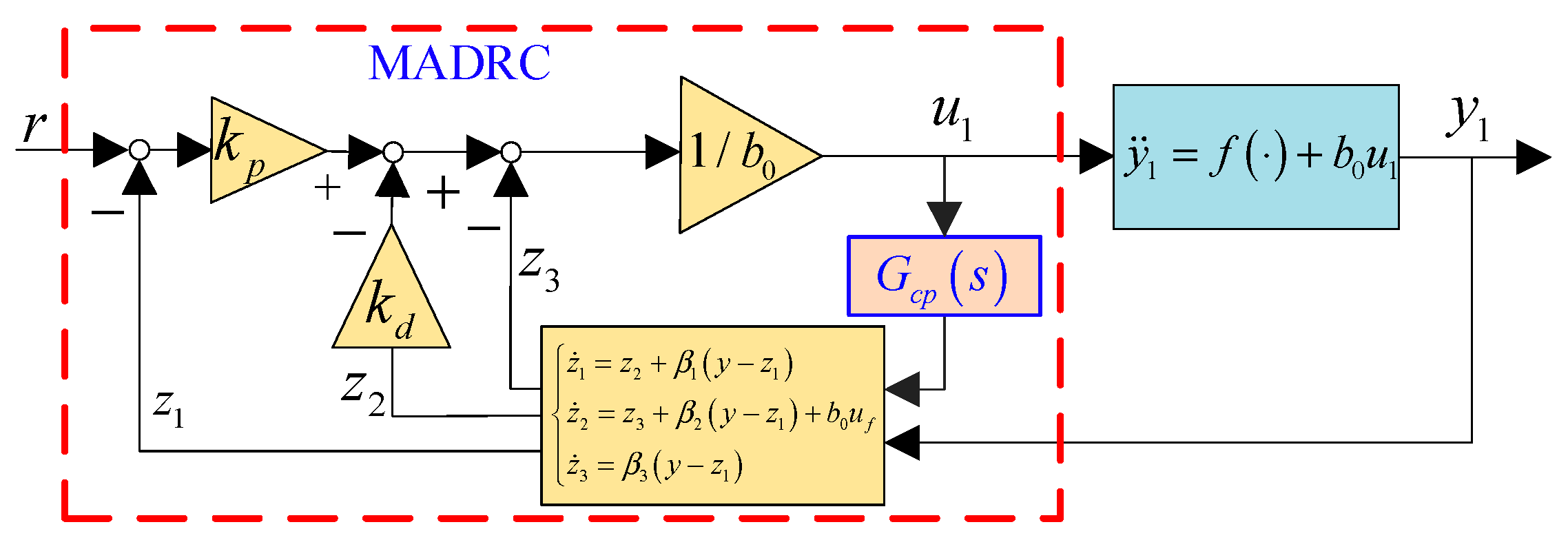
3. Modified Active Disturbance Rejection Control and Convergence Analysis

3.1. Regular Active Disturbance Rejection Control

Considering the controlled plant, $G_{out-loop}(s)$, in Equation (15) for $G_{c1}\left(s\right)$, the controlled plant can be equivalent to

$${\ddot{y}}_1=-\frac{{\dot{y}}_1}{30}+\frac{1}{30}{u}_1.$$

(18)

In order to maintain generality, Equation (18) can have the general form

$${\ddot{y}}_1=g\left(\dot{y},y,\omega ,d\right)+b{u}_1,$$

(19)

where $t$, $\omega$ and $d$ are the time variation, system uncertainties and external disturbances, respectively. In addition, $b$ is the gain of $u$ and $b=1/30$ for Equation (15). Note that Equation (15) is an approximation of Equation (14) and the accurate gain has some changes. Therefore, $b_0$, defined as the estimation of $b$, is used in Equation (19), and Equation (19) becomes

$${\ddot{y}}_1=\underset{f\left(\cdot \right)}{\underbrace{g\left(\dot{y},y,\omega ,d\right)+\left(b-b_0\right)u_1}}+b_0{u}_1,$$

(20)

where $f\left(\cdot \right)=g\left(\dot{y},y,\omega ,d\right)+\left(b-b_0\right)u_1$ is called the total disturbance of the controlled plant, and it contains external disturbances and internal uncertainties.

To estimate $f\left(\cdot \right)$, ESO is proposed for Equation (20), which is depicted by

$$\left\{\begin{array}{l}{\dot{z}}_1=z_2+{\beta }_1\left(y_1-z_1\right)\\ {\dot{z}}_2=z_3+{\beta }_2\left(y_1-z_1\right)+b_0{u}_1\\ {\dot{z}}_3={\beta }_3\left(y_1-z_1\right)\end{array}\right.,$$

(21)

where $z_1$, $z_2$ and $z_3$ are the outputs of ESO. ${\beta }_1$, ${\beta }_2$ and ${\beta }_3$ denote parameters of ESO, and the parameter-bandwidth method is proposed to simplify parameter tuning as [37]:

$$\left\{\begin{array}{l}{\beta }_1=3{\omega }_o\\ {\beta }_2=3{\omega }_o^2\\ {\beta }_3={\omega }_o^3\end{array}\right.,$$

(22)

where ${\omega }_o$ is the bandwidth of ESO. Note that $z_1$, $z_2$ and $z_3$ can track $y$, $\dot{y}$ and $f\left(\cdot \right)$ well when ${\beta }_1$, ${\beta }_2$ and ${\beta }_3$ are tuned reasonably [23].

A feedback control law is designed to obtain the control signal as

$$u_1=\frac{k_p\left(r-z_1\right)-k_p{z}_2-z_3}{b_0},$$

(23)

where $k_p$ and $k_d$ are parameters of the feedback control law, which can be decided by

$$\left\{\begin{array}{l}{k}_p={\omega }_c^2\\ k_d=2{\omega }_c\end{array}\right.,$$

(24)

where ${\omega }_c$ is the bandwidth of the feedback control law. The structure of the regular ADRC can be seen in Figure 5.

3.2. Modified Active Disturbance Rejection Control

Due to the inertial link in Equation (15), the inputs of ESO, i.e., $u_1$ and $y_1$, are un-synchronized, and this can limit the upper limit of ESO. To resolve the issue, a synchronized part, i.e., $G_{cp}\left(s\right)=\frac{1}{30s+1}$, is added to $u_1$ before $u_1$ is sent to ESO as presented in Figure 6. Thus, $u_1$, as one input of ESO, is replaced by the output, i.e., $u_f$, of $G_{cp}\left(s\right)$. ESO and the feedback control law are the same as those of the regular ADRC. Note that the parameter-bandwidth method for ${\omega }_o$ and ${\omega }_c$ is still effective for the MADRC.

The controlled plant in Equation (14) becomes,

$$Y_1(s)=\frac{0.74\left(k_{d1}{s}^2+k_{p1}s+k_{i1}\right)}{s\left[\left(0.348k_{d1}+5\right)s^2+\left(0.348k_{p1}+1\right)s+0.348k_{i1}\right]}{u}_f(s),$$

(25)

which is equivalent to

$${\ddot{y}}_1=f\left(\cdot \right)+{\tilde{b}}_0{u}_f.$$

(26)

Note that $b_0$ in the ESO and the feedback control law of the regular ADRC is replaced by ${\tilde{b}}_0$. The structure of the modified ADRC in Figure 6 is equivalent to a typical two-degrees-of-freedom structure as presented in Figure 7, where $G_P\left(s\right)$, $G_F\left(s\right)$ and $G_c\left(s\right)$ are the controlled plant, feedforward controller and feedback controller, respectively.

Without loss of generality, Equation (20) is considered, and the synchronized part becomes

$$G_{cp}(s)=\frac{1}{Ts+1}.$$

(27)

By equivalent transformation, $G_F\left(s\right)$ and $G_c\left(s\right)$ can be obtained as

$$G_F(s)=\frac{s^3+{\beta }_1{s}^2+{\beta }_{2}s+{\beta }_3}{\left(k_1{\beta }_1+k_2{\beta }_2+{\beta }_3\right)s^2+\left(k_1{\beta }_2+k_2{\beta }_3\right)s+k_1{\beta }_3},$$

(28)

and

$$G_C(s)=\frac{\frac{k_p}{{\tilde{b}}_0}\left(\left(k_p{\beta }_1+k_d{\beta }_2+{\beta }_3\right)s^2+\left(k_p{\beta }_2+k_d{\beta }_3\right)s+k_p{\beta }_3\right)}{s^3+\left({\beta }_1+k_d{G}_{cp}\left(s\right)\right)s^2+\left({\beta }_2+k_d{\beta }_1{G}_{cp}\left(s\right)+k_p{G}_{cp}\left(s\right)\right)s+{\beta }_3\left(1-G_{cp}\left(s\right)\right)}.$$

(29)

Thus, one has the following theorem of the stability analysis for the MADRC as follows:

Theorem 1.

Suppose that $f$ is bounded, and $r$ is independent of time. Based on the controlled plant in Equation (20) and the equivalent structure in Equations (28) and (29), the sufficient condition of the bounded tracking error $\left|y-r\right|$ is that all roots of $\left[k_p+k_{d}s+s^2\left(Ts+1\right)\right]\left(s^3+{\beta }_1{s}^2+{\beta }_{2}s+{\beta }_3\right)=0$ locate in the left plane.

Proof of Theorem 1.

The state space representation of the synchronized part can be obtained as

$${\dot{u}}_f=-\frac{1}{T}{u}_f+\frac{1}{T}{u}_1.$$

(30)

Considering that $r$ is set to zero, the closed-loop system becomes

$$\left\{\begin{array}{l}\ddot{y}={\tilde{b}}_0{u}_f+f\\ {\dot{u}}_f=-\frac{1}{T}{u}_f+\frac{1}{T}{u}_1\\ {\dot{z}}_1=z_2+{\beta }_1\left(y_1-z_1\right)\\ {\dot{z}}_2=z_3+{\beta }_2\left(y_1-z_1\right)+{\tilde{b}}_0{u}_f\\ {\dot{z}}_3={\beta }_3\left(y_1-z_1\right)\\ u_1=\frac{k_p\left(r-z_1\right)-k_d{z}_2-z_3}{{\tilde{b}}_0}\end{array}\right..$$

(31)

By defining the tracking error as $e_z=y-r$ and state estimation error as $e_1=y-z_1$, $e_2=\dot{y}-z_2$ and $e_3=f-z_3$, one can obtain

$${\dot{e}}_z=\dot{y}-\dot{r}=\dot{y}$$

(32)

and

$$\left\{\begin{array}{l}{\dot{e}}_1=e_2-{\beta }_1{e}_1\\ {\dot{e}}_2=e_3-{\beta }_2{e}_1\\ {\dot{e}}_3=\dot{f}-{\beta }_3{e}_1\end{array}\right..$$

(33)

Combining Equations (31)–(33), the overall closed-loop system becomes

$$\left\{\begin{array}{l}{\dot{e}}_z=\tilde{y}\\ \dot{y}=\tilde{y}\\ \dot{\tilde{y}}={\tilde{b}}_0{u}_f+f\\ {\dot{u}}_f=-\frac{1}{T}{u}_f-\frac{k_p}{{\tilde{b}}_{0}T}{e}_z+\frac{k_p}{{\tilde{b}}_{0}T}{e}_1-\frac{k_d}{{\tilde{b}}_{0}T}\tilde{y}+\frac{k_d}{{\tilde{b}}_{0}T}{e}_2-\\ {\dot{e}}_1=e_2-{\beta }_1{e}_1\\ {\dot{e}}_2=z_3-{\beta }_2{e}_1+f\\ {\dot{z}}_3={\beta }_3{e}_1\end{array}\right.\frac{1}{{\tilde{b}}_{0}T}{z}_3.$$

(34)

The characteristic equation of the closed-loop system in Equation (34) can be obtained as

$$\left[k_p+k_{d}s+s^2\left(Ts+1\right)\right]\left(s^3+{\beta }_1{s}^2+{\beta }_{2}s+{\beta }_3\right)=0.$$

(35)

When all roots of Equation (35) locate on the left plane, it can be learned the all eigenvalues of the closed-loop system in Equation (34) are located on the left plane. Considering that $f$ is bounded, $\left|e_z\right|=\left|y-r\right|$ is bounded. □

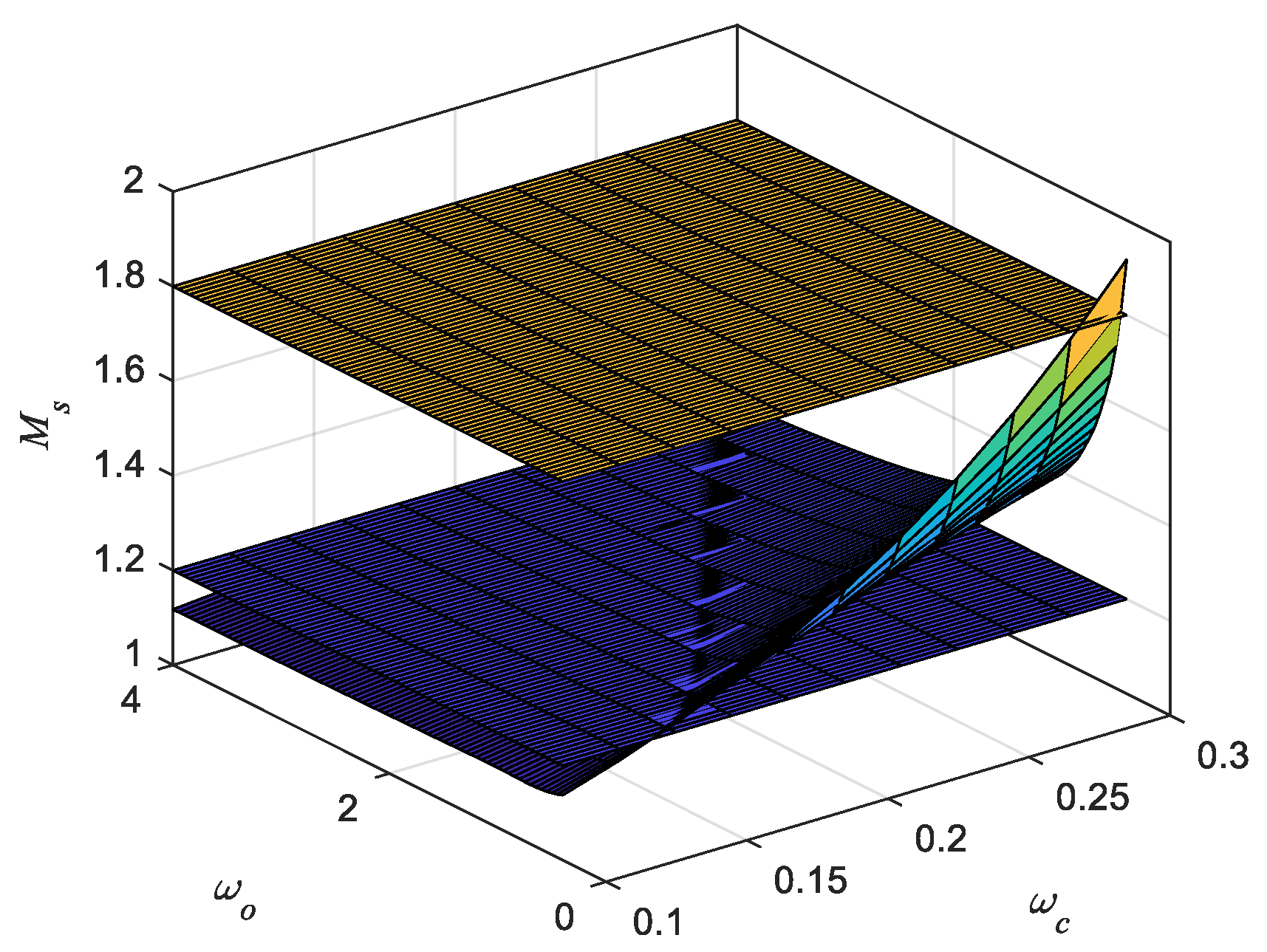
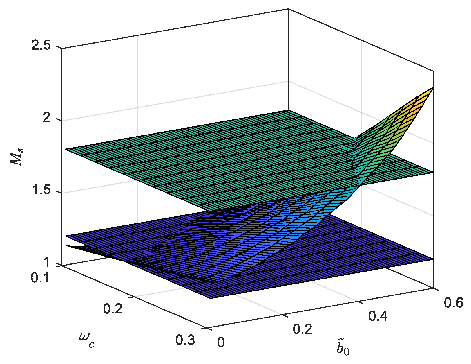
3.3. Distributions of M_s for MADRC

Theorem 1 verifies the convergence of the proposed MADRC, where the tracking error is decided by the parameters of the MADRC. To guarantee the ability to handle system uncertainties, the robustness index, $M_s$, should be a key constraint. To better analyze the influence of parameters on $M_s$, the three-dimensional distributions of $M_s$ with different {${\omega }_c$, ${\omega }_o$}, {${\omega }_c$, ${\tilde{b}}_0$} and {${\omega }_o$, ${\tilde{b}}_0$} are obtained and presented in Figure 8, Figure 9 and Figure 10, respectively.

It can be learned that the distributions of $M_s$ obviously change with different {${\omega }_c$, ${\omega }_o$}, {${\omega }_c$, ${\tilde{b}}_0$} and {${\omega }_o$, ${\tilde{b}}_0$}. This means that the parameters of the MADRC should be tuned appropriately to obtain satisfactory control performance of the drum water level for heat recovery boilers.

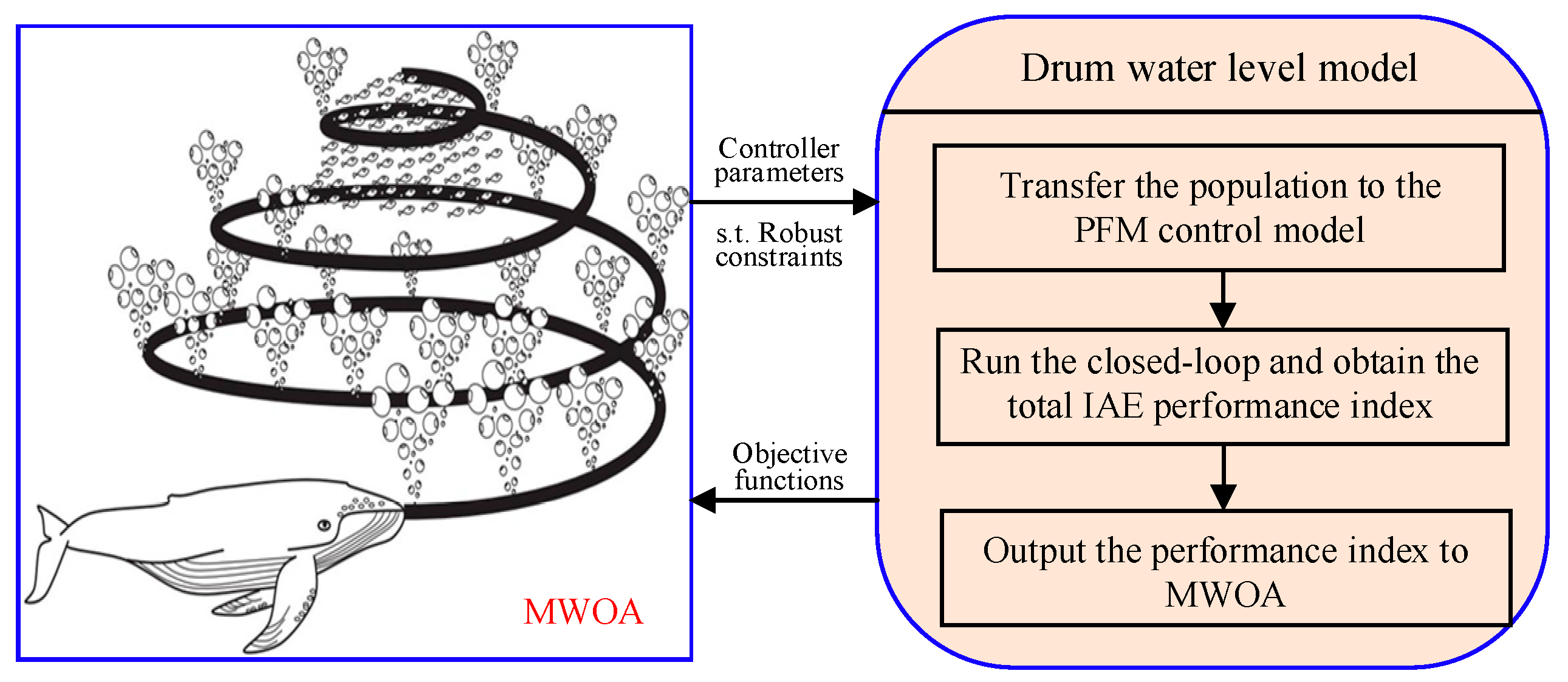
4. Modified Whale Optimization Algorithm with Sensitivity Constraint for MADRC

To optimize the parameters of the proposed MADRC, i.e., $G_{c1}\left(s\right)$, for the drum water level, MWOA is proposed to tune these parameters, considering its simplicity, efficiency and fast convergence as presented in Figure 11.

The WOA is a novel swarm intelligence optimization algorithm that mimics the predatory behavior of whales in nature [34], and the predatory behavior of whales can be mainly divided into two categories: (1) searching for food on the bubble net and (2) random search [38].

Searching for food on the bubble net: In the WOA, the position of each whale in the search space represents a solution. Assuming that the individual closest to the objective function value in the current population is the optimal whale position, based on the position information of the global optimal solution, other whale individuals in the population update their own positions by surrounding the optimal whale position. The behavior of whales surrounding prey is shown in Equation (36) as

$$x_{new}^t=x_{*}^t-A\times D,$$

(36)

where $D=\left|C\cdot x_{*}^t-x^t\right|$, $t$ is the current iteration number, $x_{*}^t$ is the global optimal whale position vector, and $x^t$ the current whale position vector.

When updating the position in a spiral, the distance between the current position and the optimal whale individual is calculated, and then the current whale swims towards the optimal individual in a spiral motion. The mathematical model is described by

$$x_{new}^t=x_{*}^t+D_p\times e^{bl}\times \cos (2\tau l),$$

(37)

where $D_p=\left|x_{*}^t-x^t\right|$, $b$ is a constant to constrain the shape of a helix, and $l\in \left[-1,1\right]$ is a random number.

Whales swim in a spiral shape towards their prey while also approaching it in a contracting manner, known as bubble-net foraging. When $\left|A\right|<1$, whales search for local optima within the enclosure and implement surround prey behavior with a probability of 0.5., and spiral renewal behavior is as follows:

$$x_{new}^t=\left\{\begin{array}{l}{x}_{*}^t-A\times D,p_1<0.5\\ x_{*}^t+D_p\times e^{bl}\times \cos (2\tau l),\hspace{1em}{p}_1\ge 0.5\end{array}\right.,$$

(38)

where $p_1$ is a random locating $\left[0,1\right]$.

Random search: When $\left|A\right|\ge 1$, whales search for optimization outside the contraction envelope and perform a random search. The algorithm randomly selects a whale individual from the current whale population as the global optimal solution, and other whales in the population gather towards it. By updating the position of the population in this way, the diversity of the whale population is enhanced, and the global search ability of the algorithm is enhanced. The mathematical model depicted by

$$x_{new}^t=x_{rand}^t-A\times D^{\prime },$$

(39)

where $D^{\prime }=\left|C\times x_{rand}^t-x^t\right|$ and $x_{rand}^t$ is a randomly selected whale position vector.

To enhance the solution accuracy and convergence speed of the WOA, the WOA is modified in the following areas:

1.

Heuristic probability $p_1$

To balance the global and local search capabilities of the WOA, the heuristic probability, i.e., $p_1$, can be calculated by

$$p_1=\left\{\begin{array}{l}0.66t_i<0.5\times \mathrm{maxIter}\\ 0.44t_i\ge 0.5\times \mathrm{maxIter}\end{array}\right.,$$

(40)

where $t_i$ and $\mathrm{maxIter}$ are the current number of iterations and the maximum number of iterations, respectively;

2.

Linear control parameter $l$

MWOA employs the linear control parameter $l$ by

$$l=\left(\frac{t}{\mathrm{maxIter}}-1\right)\times rand+1-2\times \frac{t}{\mathrm{maxIter}};$$

(41)

3.

Lévy flight strategy

The position of a whale individual can be updated by Lévy flight strategy as

$$X_{\mathrm{new}}^i=X^i+A_1\times \frac{\upsilon }{{\left|\mu \right|}^{1/\beta }}\oplus \left(X^i-C_1\times X^{\mathrm{rand}}\right),$$

(42)

where $X_{\mathrm{new}}^i$ is the updated position of $X^i$, $\oplus$ is the dot product, and $X^{\mathrm{rand}}$ is the randomly selected whale individual in the current population. In addition, $A_1$ and $C_1$ are two parameters [34];

4.

Elementary knowledge-acquisition-sharing algorithm

The position of a whale individual can be updated by the elementary knowledge-acquisition-sharing algorithm as

$$X_{\mathrm{new}}^i=\left\{\begin{array}{l}{X}^i+k_f\times \left[\left(X^{i-1}-X^{i+1}\right)+\left(X^r-X^i\right)\right]\hspace{1em}m\left(X^i\right)>m\left(X^r\right)\\ X^i+k_f\times \left[\left(X^{i-1}-X^{i+1}\right)+\left(X^i-X^r\right)\right]\hspace{1em}m\left(X^i\right)\le m\left(X^r\right)\end{array}\right.,$$

(43)

where $X^r$, $m\left(X^i\right)$ and $k_f$ are the randomly selected individuals, the fitness function of $X^i$ and knowledge factor parameters, respectively;

5.

Position update method based on correction spiral

The position of a whale individual can be updated by the position update method based on the correction spiral as

$$X_{\mathrm{new}}^i=X_{*}^i+\left(X_{*}^i-X_{worst}^i+\left|X_m^i-X^i\right|\right)e^l\cos \left(2\pi l\right),$$

(44)

where $X_{*}^i$, $X_{worst}^i$ and $X_m^i$ are the best, worst and medium whale individuals, respectively;

6.

Quadratic interpolation method

The position of a whale individual can be updated by the quadratic interpolation method as

$$X_{\mathrm{new}}^i=0.5\times \frac{\left[{\left(X^i\right)}^2-{\left(X^r\right)}^2\right]\times m\left(X_{*}^i\right)+\left[{\left(X^r\right)}^2-{\left(X_{*}^i\right)}^2\right]\times m\left(X^i\right)+\left[{\left(X_{*}^i\right)}^2-{\left(X^i\right)}^2\right]\times m\left(X^r\right)}{\left(X^i-X^r\right)\times m\left(X_{*}^i\right)+\left(X^r-X_{*}^i\right)\times m\left(X^i\right)+\left(X_{*}^i-X^i\right)\times m\left(X^r\right)}.$$

(45)

The flowsheet of the MWOA can be seen in Figure 12, where more meaning of variables can be seen in Ref. [34].

With the same sensitivity constraint, i.e., $M_s=1.5$, the WOA and MWOA are applied to optimize the parameters of the MADRC for the drum water level, and the convergence curves of the control performance, i.e., IAE, can be obtained as shown in Figure 13, where the MWOA has fast convergence. In addition, the IAE with the WOA and MWOA are 30.94 and 28.17, respectively. The solution accuracy and convergence speed of the MWOA can be verified.

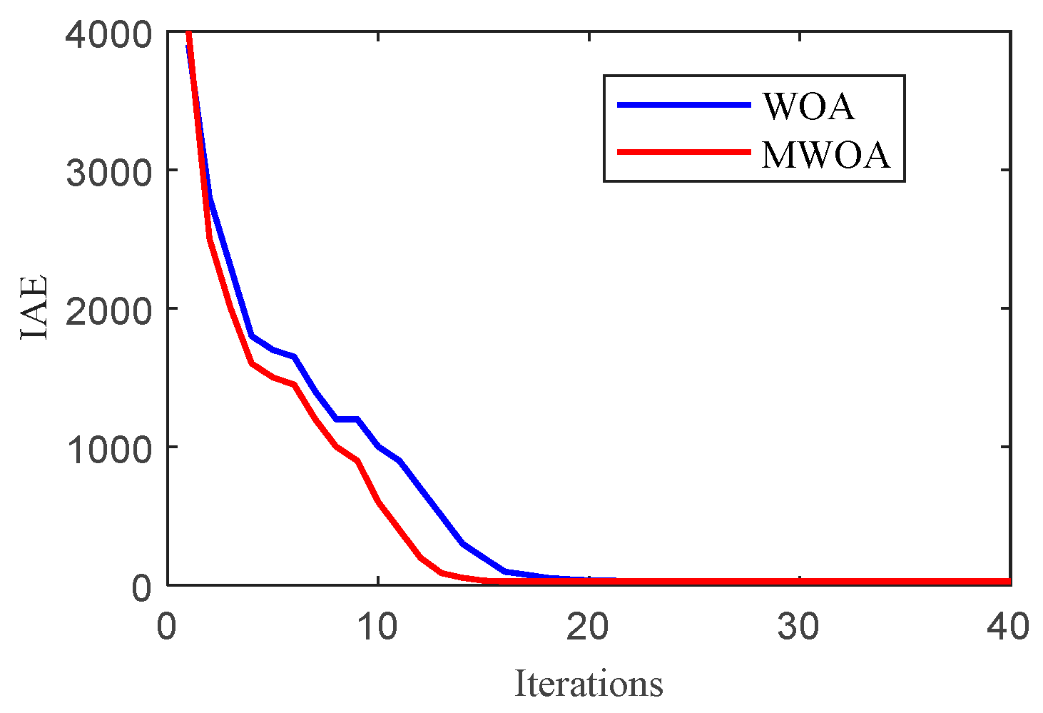
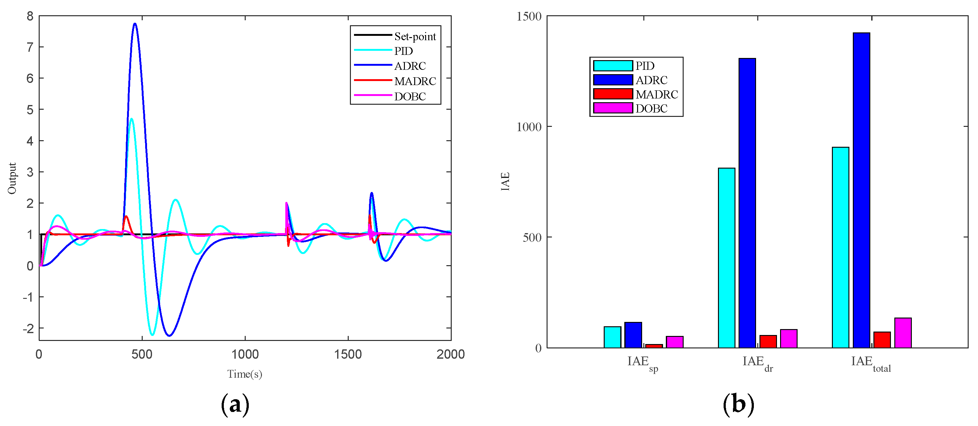
5. Simulation Illustrations

To validate the effectiveness of the proposed MADRC optimized by the MWOA, the control performance with the fixed sensitivity constraint is carried out in this scenario. Moreover, the PID, regular ADRC (“ADRC” in this paper) and disturbance observer-based control (“DOBC” in this paper) are selected as comparative controllers.

To comprehensively compare the performance of the MADRC, three scenarios are selected: (1) Scenario 1—the simulations with fixed sensitivity constraints are carried out to analyze the control performance under different constraints in this scenario; (2) Scenario 2—In this scenario, the sensitivity constraint is selected as a reasonable range to obtain better control performance; (3) Scenario 3—In this scenario, Monte Carlo simulations are carried out to compare the different controllers’ ability to handle system uncertainties.

In addition, the IAE is selected as the indicator to measure the control performance of these controllers considering that it can balance control accuracy and convergence speed well [36]. The definition of IAE can be depicted by

$$\mathrm{IAE}={\displaystyle {\int }_{t_{start}}^{t_{end}}\left|r(t)-y(t)\right|dt},$$

(46)

where $t_{start}$ and $t_{end}$ are the start time and end time of the calculation process, respectively. If $t_{start}$ and $t_{end}$ are selected as the start time and end time of the tracking process, the IAE becomes the set-point tracking performance IAE_sp. Similarly, the IAE becomes the disturbance rejection performance IAE_dr if $t_{start}$ and $t_{end}$ are selected as the start time and end time of the disturbance rejection process. The IAE becomes the total performance IAE_total if $t_{start}$ and $t_{end}$ are selected as the start time and end time of the simulation process.

5.1. Scenario 1: Fixed Sensitivity Constraint

Select a fixed sensitivity constraint, i.e., $M_s=1.2$, and the parameters of the inner controller, i.e., $G_{c2}\left(s\right)$, are given as $G_{c2}\left(s\right)=0.8+0.01/s$. Then MWOA is applied to the MADRC, PID and ADRC. The parameters of the MADRC are obtained as ${\tilde{b}}_0=0.00198$, ${\omega }_c=0.168$ and ${\omega }_o=0.996$. The parameters of the ADRC are obtained as $b_0=0.102$, ${\omega }_c=0.0172$ and ${\omega }_o=0.899$. The parameters of the PID are obtained as $k_p=0.148$, $k_i=0.00497$ and $k_d=5.489$. The parameters of the DOBC are obtained as $k_p=1.193$, $k_i=0.0272$, $k_d=107.1210$ and $Q\left(s\right)=1/{(8s+1)}^2$. The control performance under the sensitivity constraint, i.e., $M_s=1.2$, is shown in Figure 14, where the set point of $y_1$ has a step change at 10 s from 0 to 1. $d_2$, $d_1$ and $D\left(s\right)$ have a step change from 0 to 1 at 400 s, 1200 s and 1600 s, respectively, during all simulations. It can be learned that the MADRC has the smallest IAEsp, IAEdr and IAE. In addition, the overshoot of the MADRC is still the smallest.

With different sensitivity constraints, i.e., $M_s=1.4$ and $M_s=1.6$, the control performance is shown in Figure 15 and Figure 16, respectively. It can be observed that the MADRC still has the best control performance compared with the ADRC, PID and DOBC, where the MADRC has the fastest tracking performance and strongest disturbance rejection ability. Note that the output of the MADRC has severe oscillations with increasing $M_s=1.6$ and this may cause wear and tear on the actuators, which is not conducive to the long-term safe operation of the drum water level for heat recovery boilers.

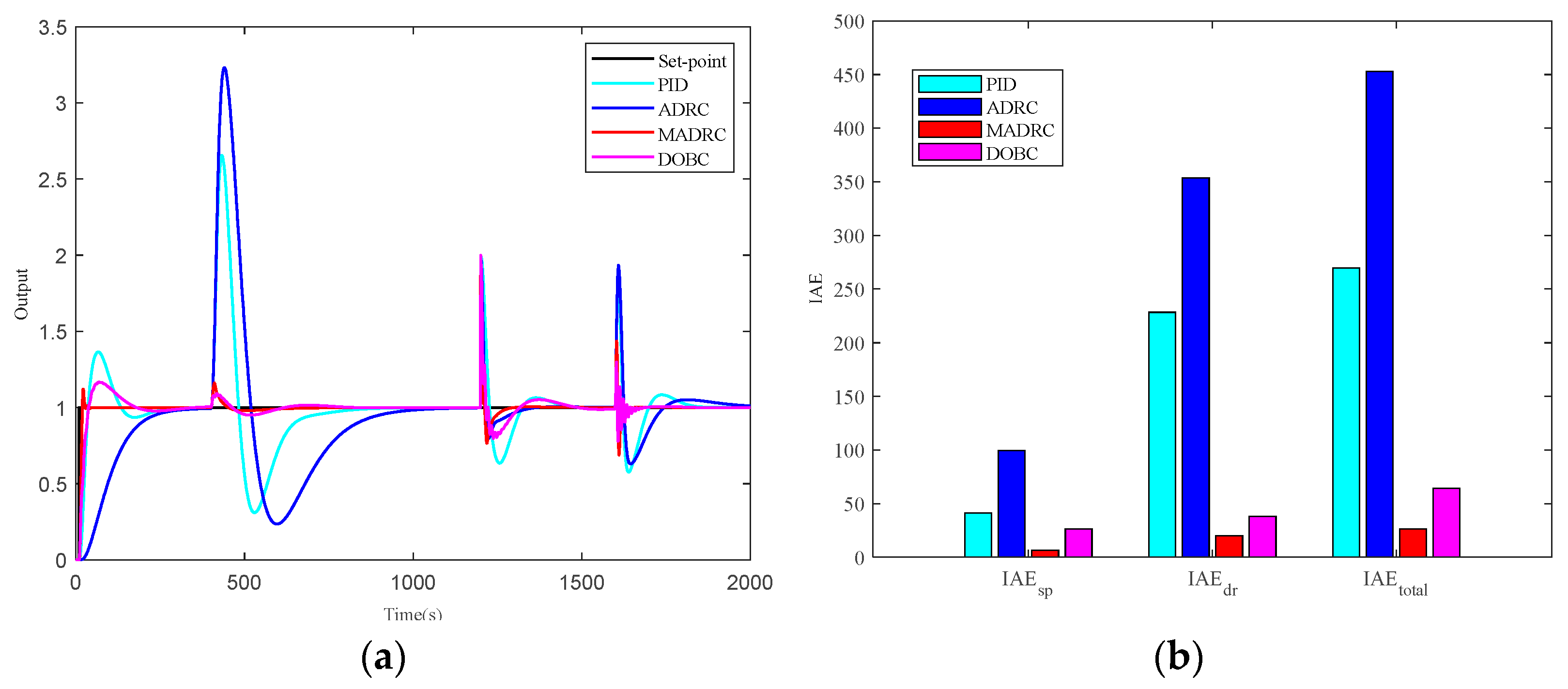
5.2. Scenario 2: Sensitivity Constraint with a Range

In this scenario, the sensitivity constraint is selected as a range, where $M_s\in \left[1.2,2.0\right]$ is selected. However, due to the severe oscillations with $M_s=1.6$ as discussed in scenario 1, $M_s$ is selected as a smaller range of $M_s\in \left[1.2,1.35\right]$ to protect actuators. With the range of the sensitivity constraint, parameters of the MADRC, PID and ADRC are optimized by the MWOA, where the parameters of the MADRC are obtained as ${\tilde{b}}_0=0.00208$, ${\omega }_c=0.214$ and ${\omega }_o=1.589$. The parameters of the ADRC are obtained as $b_0=0.0973$, ${\omega }_c=0.0493$ and ${\omega }_o=3.02$. The parameters of the PID are obtained as $k_p=2.10$, $k_i=0.0199$ and $k_d=30$. The parameters of the DOBC are obtained as $k_p=3.07$, $k_i=0.0310$, $k_d=120$ and $Q\left(s\right)=1/{(8s+1)}^2$. The control performance under a range sensitivity constraint is shown in Figure 17. It can be learned that the MADRC has the smallest IAEsp, and the MADRC has smaller IAEdr and IAE than the PID and ADRC. In addition, the overshoot of the MADRC is still the smallest. In addition, the Nyquist plots of different controllers are presented in Figure 18, where the MADRC has the smallest $M_s$, while the DOBC, ADRC and PID have a larger $M_s$.

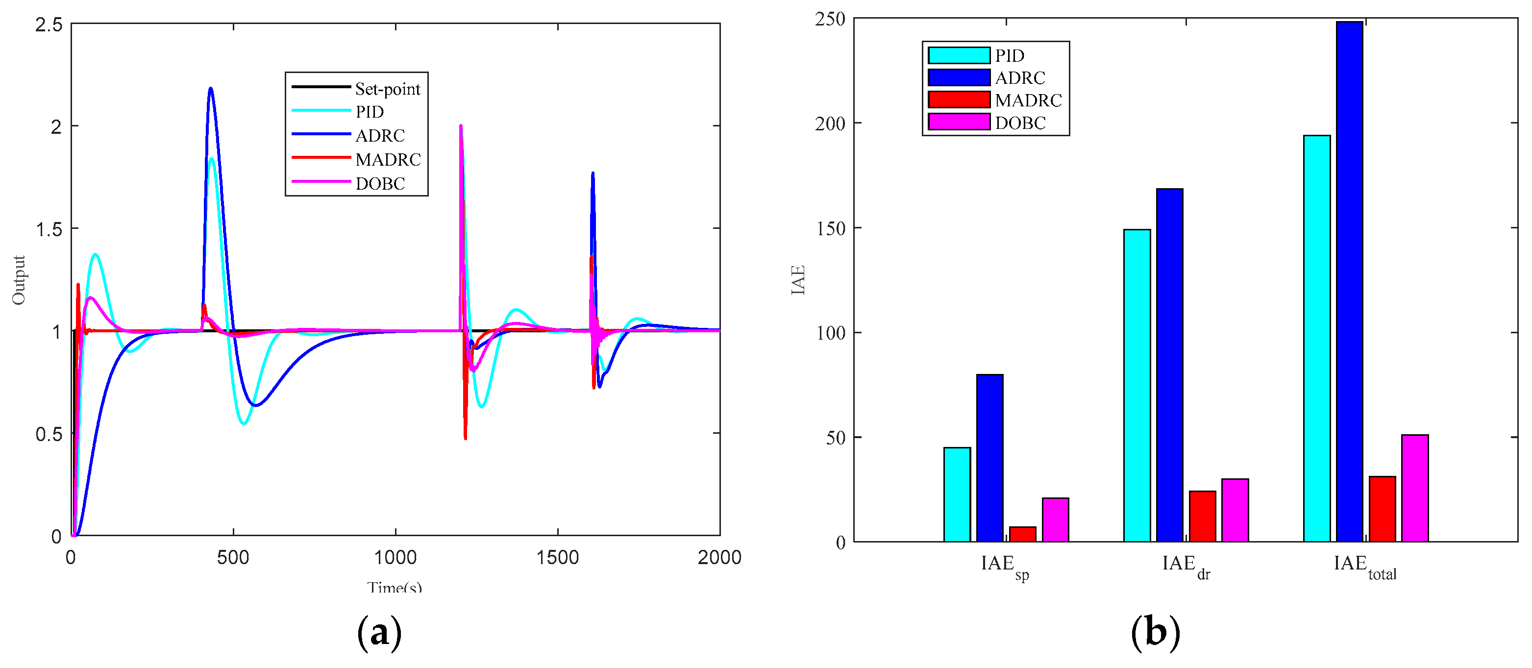
5.3. Scenario 3: Uncertain Systems

Considering that system uncertainties always exist with changing operating conditions and model simplification, to analyze the abilities of the MADRC, DOCB, ADRC and PID to handle system uncertainties for the drum water level, Monte Carlo simulations are carried out in scenario 3.

All coefficients in Figure 1 are perturbed in the [−20%, 20%] range of their original values randomly, and then simulations in Figure 14 are carried out for perturbed systems with fixed parameters. During each simulation, the IAE_sp, IAE_dr and IAE are recorded. By repeating simulations 200 times for scenarios 1 and 2, the distributions of the IAE_sp, IAE_dr and IAE are presented in Figure 19.

Commonly, the control performance is better if the controller has smaller IAE_sp, IAE_dr and IAE; similarly, the robustness is strong if the controller has a greater concentration of the IAE_sp, IAE_dr and IAE. It can be learned that the MADRC has the best control performance and strongest robustness for uncertain systems, which means that the MADRC has the strongest ability to handle system uncertainties.

Based on simulation results, the MADRC obtains obvious advantages in terms of tracking performance and disturbance rejection ability with satisfactory robustness.

6. Conclusions

This paper focuses on the controller design for the drum water level, where external disturbances and system uncertainties are the main challenges to the control of drum water level. An MADRC optimized by an MWOA with sensitivity constraint is proposed. Based on the control structure of a three-element control system for the drum water level and the regular ADRC structure, the structure of an MADRC is introduced and the convergence of the proposed MADRC is derived. Then a modified whale optimization algorithm (MWOA) with sensitivity constraint is applied to optimize the parameters of the MADRC. Simulation results and performance indexes show that the proposed MADRC can obtain the best tracking and disturbance rejection abilities with satisfactory robustness. The satisfactory control performance shows that the proposed MADRC has wide application potential for heat recovery boilers and other industrial processes.

References

1. Arpit, S.; Das, P.K. A state-of-the-art review of heat recovery steam generators and waste heat boilers. Energy Effic. 2023, 16, 99. [Google Scholar] [CrossRef]
2. Moradi, H.; Saffar-Avval, M.; Bakhtiari-Nejad, F. Sliding mode control of drum water level in an industrial boiler unit with time varying parameters: A comparison with H∞-robust control approach. J. Process Control 2013, 22, 1844–1855. [Google Scholar] [CrossRef]
3. Xiao, B.; Xie, A.; Xiao, M.; Zhou, M.; Su, S.; Xiao, Z.; Li, X. Optimal design of boiler drum water level control system. In Proceedings of the Third International Conference on Mechanical, Electronics, and Electrical and Automation Control (METMS 2023), Hangzhou, China, 17–19 February 2023. [Google Scholar] [CrossRef]
4. Thampi, M.S.P.; Raghavendra, G. Intelligent model for automating PID controller tuning for industrial water level control system. In Proceedings of the 2021 International Conference on Design Innovations for 3Cs Compute Communicate Control (ICDI3C), Bangalore, India, 10–11 June 2021. [Google Scholar] [CrossRef]
5. Liu, J.; Sun, W.; Zhang, S. Particle swarm optimization-based PID control of drum water level. Comput. Eng. App. 2009, 45, 239–241. [Google Scholar]
6. Zhao, X. Chaos optimization strategy on fuzzy adaptive PID control of boiler drum water level. In Proceedings of the Annual Conference of China-Institute-of-Communications, Guangzhou, China, 26 November 2009. [Google Scholar]
7. Liu, C.; Chen, M. Research on fuzzy PID control of boiler drum water level. J. Eng. Therm. Energy Power 2021, 36, 100–105. [Google Scholar]
8. Precup, R.E.; Nguyen, A.T.; Blazic, S. A survey on fuzzy control for mechatronics applications, Int. J. Syst. Sci. 2023, 55, 771–813. [Google Scholar] [CrossRef]
9. Elhosseini, M.A.; El-din, A.S.; Ali, H.A.; Abraham, A. Heat recovery steam generator (HRSG) three-element drum level control utilizing fractional order PID and fuzzy controllers. ISA Trans. 2022, 122, 281–293. [Google Scholar] [CrossRef]
10. Shah, P.; Agashe, S. Review of fractional PID controller. Mechatronics 2016, 38, 29–41. [Google Scholar] [CrossRef]
11. Ahooghalandari, N.; Shadi, R.; Fakharian, A. Hinfinity robust control design for three-element industrial boiler supervisory system. In Proceedings of the 2022 8th International Conference on Control, Instrumentation and Automation (ICCIA), Tehran, Iran, 2–3 March 2022. [Google Scholar] [CrossRef]
12. Moradi, H.; Bakhtiari-Nejad, F.; Saffar-Awal, M. Robust control of an industrial boiler system; a comparison between two approaches: Sliding mode control & H∞ technique. Energy Conv. Manag. 2009, 50, 1401–1410. [Google Scholar]
13. Panda, S.K.; Subudhi, B. A review on robust and adaptive control schemes for microgrid. J. Mod. Power Syst. Clean Energy 2023, 11, 1027–1040. [Google Scholar] [CrossRef]
14. Wu, Z.L.; Li, D.H.; Chen, Y.Q. Active Disturbance rejection control design based on probabilistic robustness for uncertain systems. Ind. Eng. Chem. Res. 2020, 59, 18070–18087. [Google Scholar] [CrossRef]
15. Pu, C.P.; Ren, J.; Su, J.B. The sliding mode control of the drum water level based on extended state observer. IEEE Access 2019, 7, 135942–135948. [Google Scholar] [CrossRef]
16. Aliakbari, S.; Ayati, M.; Osman, J.H.S.; Sam, Y.M. Second-order sliding mode fault-tolerant control of heat recovery steam generator boiler in combined cycle power plants. Appl. Therm. Eng. 2013, 50, 1326–1338. [Google Scholar] [CrossRef]
17. Li, B.; Guo, F.; Jia, W.; Zhao, Q. Application research on grey generalized prediction control in boiler drum water level. Comput. Meas. Control 2010, 18, 370–406. [Google Scholar]
18. Sun, L.F.; Li, J.C.; Zhao, X. Predictive control of drum water level based on ant colony optimization algorithm. In Proceedings of the 29th Chinese Control Conference, Beijing, China, 29–31 July 2010. [Google Scholar]
19. Urrea, C.; Paez, F. Design and comparison of strategies for level control in a nonlinear tank. Processes 2021, 9, 735. [Google Scholar] [CrossRef]
20. Quan, Y.L.; Yang, X.H. A method for alarming water level of boiler drum on nuclear power plant based on BP neural network. In Proceedings of the 2014 10th International Conference on Natural Computation (ICNC), Xiamen, China, 19–21 August 2014. [Google Scholar]
21. Panjapornpon, C.; Chinchalongporn, P.; Bardeeniz, S.; Makkayatorn, R.; Wongpunnawat, W. Reinforcement learning control with deep deterministic policy gradient algorithm for multivariable ph process. Processes 2022, 10, 2514. [Google Scholar] [CrossRef]
22. Wu, Z.L.; Gao, Z.Q.; Li, D.H.; Chen, Y.Q.; Liu, Y.H. On transitioning from PID to ADRC in thermal power plants. Control Theory Technol. 2021, 19, 3–18. [Google Scholar] [CrossRef]
23. Xue, W.C.; Huang, Y. Performance analysis of active disturbance rejection tracking control for a class of uncertain LTI systems. ISA Trans. 2015, 58, 133–154. [Google Scholar] [CrossRef]
24. Gao, B.W.; Zheng, L.T.; Shen, W.; Zhang, W. A summary of parameter tuning of active disturbance rejection controller. Recent. Adv. Electr. Electron. Eng. 2023, 16, 180–196. [Google Scholar]
25. Fareh, R.; Khadraoui, S.; Abdallah, M.Y.; Baziyad, M.; Bettayeb, M. Active disturbance rejection control for robotic systems: A review. Mechatronics 2021, 80, 102671. [Google Scholar] [CrossRef]
26. Wu, Z.L.; Li, D.H.; Liu, Y.H.; Chen, Y.Q. Performance analysis of improved ADRCs for a class of high-order processes with verification on main steam pressure control. IEEE Trans. Ind. Electron. 2023, 70, 6180–6190. [Google Scholar] [CrossRef]
27. Wu, Z.L.; He, T.; Li, D.H.; Xue, Y.L.; Sun, L.; Sun, L.M. Superheated steam temperature control based on modified active disturbance rejection control. Control Eng. Pract. 2019, 83, 83–97. [Google Scholar] [CrossRef]
28. Wang, P.Y.; Zhang, C.R.; Zhu, L.K.; Wang, C.C. The research of improved active disturbance rejection control algorithm for particleboard glue system based on neural network state observer. Algorithms 2020, 12, 259. [Google Scholar] [CrossRef]
29. Xu, F.R.; Chen, M.Q.; Liang, X.L.; Liu, W.S. PSO optimized active disturbance rejection control for aircraft anti-skid braking system. Algorithms 2022, 15, 158. [Google Scholar] [CrossRef]
30. Wu, Z.L.; Liu, Y.H.; Li, D.H.; Chen, Y.Q. Multivariable active disturbance rejection control for compression liquid chiller system. Energy 2023, 262, 125344. [Google Scholar] [CrossRef]
31. Pu, C.; Zhu, Y.; Su, J. Drum water level control based on improved ADRC. Algorithms 2019, 12, 132. [Google Scholar] [CrossRef]
32. Wang, D.; Li, H.Y.; Xie, X.Y.; Liu, D.Y. Boiler drum water level control based on linear active disturbance rejection and gray correlation compensation. Control Eng. Appl. Inform. 2020, 22, 42–49. [Google Scholar]
33. Hu, C.M.; Ren, J. Study and application of LADRC for drum water-level cascade three-element control. Electr. Power 2014, 47, 28–31. [Google Scholar]
34. Sun, Y.J.; Wang, X.L.; Chen, Y.H.; Liu, Z.J. A modified whale optimization algorithm for large-scale global optimization problems. Expert Syst. Appl. 2018, 114, 563–577. [Google Scholar] [CrossRef]
35. Astrom, K.J.; Panagopoulos, H.; Hagglund, T. Design of PI controllers based on non-convex optimization. Automatica 1998, 34, 585–601. [Google Scholar] [CrossRef]
36. Wu, Z.L.; Li, D.H.; Xue, Y.L. A new PID controller design with constraints on relative delay margin for first-order plus dead-time systems. Processes 2019, 7, 713. [Google Scholar] [CrossRef]
37. Gao, Z.Q. Scaling and bandwidth-parameterization based controller tuning. In Proceedings of the American Control Conference, Denver, CO, USA, 4–6 June 2003. [Google Scholar] [CrossRef]
38. Mirjalili, S.; Lewis, A. The whale optimization algorithm. Adv. Eng. Softw. 2016, 95, 51–67. [Google Scholar] [CrossRef]
Figure 1. The control structure of the drum water level.
Energies 17 01438 g001
Figure 2. The inner loop and outer loop are divided into a three-element system.
Energies 17 01438 g002
Figure 3. The equivalent structure of the drum water level in Figure 1.
Energies 17 01438 g003
Figure 4. Graph understanding of the maximum sensitivity function.
Energies 17 01438 g004
Figure 5. The structure of the regular ADRC.
Energies 17 01438 g005
Figure 6. The structure of the modified ADRC.
Energies 17 01438 g006
Figure 7. The equivalent structure of the modified ADRC.
Energies 17 01438 g007
Figure 8. Distributions of M s with different ω c and ω o .
Energies 17 01438 g008
Figure 9. Distributions of M s with different ω c and b ˜ 0 .
Energies 17 01438 g009
Figure 10. Distributions of M s with different ω o and b ˜ 0 .
Energies 17 01438 g010
Figure 11. The diagrammatic sketch of MWOA applying to the drum water level.
Energies 17 01438 g011
Figure 12. The flowsheet of MWOA.
Energies 17 01438 g012
Figure 13. The convergence curves of IAE with WOA and MWOA ( M s = 1.5 ).
Energies 17 01438 g013
Figure 14. The control performance under the sensitivity constraint, i.e., M s = 1.2 . (a) The outputs with different controllers; (b) the control performance indexes with different controllers.
Energies 17 01438 g014
Figure 15. The control performance under the sensitivity constraint, i.e., M s = 1.4 . (a) The outputs with different controllers; (b) the control performance indexes with different controllers.
Energies 17 01438 g015
Figure 16. The control performance under the sensitivity constraint, i.e., M s = 1.6 . (a) The outputs with different controllers; (b) the control performance indexes with different controllers.
Energies 17 01438 g016
Figure 17. The control performance under the sensitivity constraint, i.e., M s 1.2 , 2.0 . (a) The outputs with different controllers; (b) the control performance indexes with different controllers.
Energies 17 01438 g017
Figure 18. The Nyquist plots of different controllers for scenario 2.
Energies 17 01438 g018
Figure 19. The distributions of IAEsp and IAEdr in Monte Carlo simulations. (a) M s = 1.2 ; (b) M s = 1.4 ; (c) M s = 1.6 ; (d) scenario 2.
Energies 17 01438 g019
Disclaimer/Publisher’s Note: The statements, opinions and data contained in all publications are solely those of the individual author(s) and contributor(s) and not of MDPI and/or the editor(s). MDPI and/or the editor(s) disclaim responsibility for any injury to people or property resulting from any ideas, methods, instructions or products referred to in the content.