Abstract
Metering anomalies not only mean huge economic losses but also indicate the faults of equipment and power lines, especially within the substation. As a result, metering anomaly diagnosis is becoming one of the most important missions in smart grids. However, due to the insufficient and imbalanced anomaly cases, identifying the anomalies in smart meter data accurately and efficiently remains challenging. Existing methods usually employ few-shot learning models in computer vision directly, which requires the rich experience of human experts and sufficient abnormal cases for training. It blocks model generalizing to various application scenarios. To address these shortcomings, we propose a novel framework for metering anomaly diagnosis based on few-shot learning, named FSMAD. Firstly, we design a fault data injection model to emulate anomalies, so that no abnormal samples are required in the training phase. Secondly, we provide a learnable variable transformation to reveal inherent relationships among various smart meter data and help FSMAD extract more efficient features. Finally, the deeper metric network is equipped to support FSMAD in obtaining powerful comparison capability. Extensive experiments on a real-world dataset demonstrate the advantages of our FSMAD over state-of-the-art methods.
1. Introduction
Electricity has become an integral part of people’s lives. Due to the growing demand for electricity, it is urgent to construct a safe, reliable, cost-effective, and environmentally friendly smart grid. Substations, as a crucial component of the smart grid, play an irreplaceable role in power generation, transmission, and distribution. Therefore, status monitoring and fault diagnosis of substations is a crucial objective of the smart grid [1,2].
Smart meters, along with communication networks and database systems, constitute the Advanced Metering Infrastructure (AMI), which plays an important role in the smart grid [3]. Particularly, any fault of the meters in the substation can lead to huge economic losses. Meanwhile, the Smart Meter (SM) data also reflect the status of the substation. Any data anomaly is directly related to the failure of substation equipment or power transmission lines [1]. Hence, the implementation of anomaly diagnosis of SM data can support the rapid location of faults and analyze the causes.
Traditionally, fault diagnosis mainly relies on expert systems [4], which use domain knowledge, expert experience, and simple machine learning methods to establish a set of indicators and parameters to identify faults [5,6]. In recent years, more and more researchers have applied artificial intelligence to the study of metering anomaly diagnosis, mainly including machine learning methods [7] and deep learning methods [8]. There are also some studies that use a combination of domain knowledge and deep learning to address the generalization performance of models [9,10]. However, due to the large number and wide distribution of smart meters, the characteristics of SM data vary widely, and metering anomaly diagnosis still faces the following challenges:
- The number of labelled samples is limited and cannot meet the training requirements of the diagnostic model;
- The distribution of anomaly categories is extremely imbalanced, resulting in the metering anomaly diagnostic model being easily overfitted;
- The traditional expert experience is not fully adapted to new application scenarios.
To address the above challenges, this article proposes a novel Few-Shot Learning-based Metering Anomaly Diagnosis (FSMAD) method. First, a set of fault data injection models (FDI) are established to simulate abnormal data by transforming normal data. This can greatly alleviate the problem of the scarcity of anomaly samples. Second, we design a mechanism to mine the physical dependencies between different variables of SM data, exceeding the limitation of experts’ experience and learning higher-quality features. Finally, we adopt a few-shot learning strategy to train the comparison ability of the model and avoid the abnormal sample imbalance problem. In summary, the main contributions of this paper specifically include:
- We present a framework FSMAD for diagnosing anomalies in power metering based on few-shot learning. For extreme situations, we establish fault data injection models to generate anomaly data. It allows us to optimize the model without any real abnormal samples and achieve a satisfying performance.
- We offer a physical dependency learning method for SM data variables. It aims to learn inherent physical relationship among variables to overcome the experience of human experts.
- We conduct comprehensive studies using real electricity metering datasets. The results of the experiment demonstrate that our metering anomaly diagnostic approach has outstanding performance.
The rest of the paper is organized as follows. Section 2 describes the related work associated with metering anomaly diagnosis. Section 3 briefly explains the power metering principles and anomalies. Section 4 presents a detailed framework and optimization algorithm of our FSMAD. Extensive experiments are conducted in Section 5 to evaluate the effectiveness of our framework. Finally, Section 6 summarizes the paper.
2. Related Work
2.1. Anomaly Diagnosis Methods
Metering anomaly diagnosis is used to accurately classify abnormal metering data, which belongs to the typical multi-classification task. For different application scenarios, a variety of different diagnostic techniques have been proposed, which have roughly gone through three stages of development: (1) expert systems; (2) machine learning; and (3) deep learning.
The expert system is an important branch of artificial intelligence. It aims to emulate the decision-making ability of human experts and solve complex problems. Expert systems are primarily composed of domain knowledge, expert experience, and reasoning techniques [11]. Yang et al. developed a method for automatically diagnosing and localizing metering anomalies by calculating indicators such as bus power imbalance, main transformer power loss, and contact line loss based on accumulated expert experience [12]. Jiang et al. developed an expert system for grid fault diagnosis. This system establishes the relationship between fault outputs and system components offline before reasoning online for confirmation [13]. Xue et al. utilized a combination of fuzzy Petri nets and expert systems to diagnose faults in power information systems, leading to improved diagnostic efficiency [4]. However, the rules of the expert system are formulated by human experts, and its effectiveness largely depends on the subjective knowledge and experience of the experts. In addition, it is also influenced by geography, weather, and time, so there are some difficulties in implementation [14].
With the advancement of data mining technology, an increasing number of machine learning methods are being applied for fault diagnosis. Wu et al. employed an improved k-means clustering algorithm [15]. The algorithm calculates the distance of the sample to the center of each anomaly cluster to determine the category of anomaly. Zhou et al. applied decision trees for meter state detection and proposed a fault diagnosis model based on tree group [16]. Since a decision tree is easy to implement, the model is well-suited for classifying anomalies in large-scale data. However, the decision tree is more sensitive to the training data, and the generalization of the model is weak. Bernat et al. compared various supervised learning methods [17]. Through a large number of experiments, researchers found that supervised learning algorithms usually show good performance when the features are of high quality. Traditional machine learning methods are unable to generate distinctive features, and the performance of fault diagnosis is limited by the quality of the features. However, feature modeling is a highly complex task, and the effectiveness of manual modeling cannot meet the demands of extensive data analysis.
Recently, due to deep learning’s ability to automatically learn the representation from raw data [18,19], it has dramatically improved the efficiency of feature modeling. As a result, it has been widely applied in fault diagnosis. Initially, a large number of studies utilized deep learning approaches directly in Computer Vision (CV) and Natural Language Processing (NLP). For example, Wen et al. converted raw signals into images and utilized image classification for fault diagnosis [20]. Shao et al. [21] and Wu et al. [22] employed auto-encoder, one-dimensional convolution, and recurrent networks for sample classification, respectively. However, the performance of these approaches is limited because the industrial signal is different from the image or language sequence. They are unable to reveal knowledge directly from the raw SM data, which means they cannot guarantee the quality of features extracted from limited samples.
To address the above problem, Zhou et al. proposed a smart meter fault diagnosis model based on an enhanced capsule network by utilizing the historical fault information of smart meters [14]. Ren et al. proposed a feature information characterization method based on fault knowledge, and then utilized recurrent neural networks to build a secondary equipment fault location model [23]. Morais et al. examined the temporal characteristics of power data and multiple sources of data [24]. They developed a diagnostic framework that utilized convolution networks and recurrent networks to identify faults. Kou et al. assembled recurrent networks and decision trees using Adaboost to improve the effectiveness of fault diagnosis [25]. Ref. [10] leverages the domain knowledge of electric energy metering to convert the SM data into classical indicators. By incorporating domain knowledge into the neural network, the performance of anomaly detection was enhanced. However, the analysis presented in the paper reveals that these metrics based on domain knowledge still cannot reliably distinguish all anomalous samples, posing a risk of failure in certain application scenarios. Therefore, deep neural networks must be able to discover the inherent dependencies among various types of data and learn more effective “indicators” from massive datasets.
2.2. Few-Shot Learning
The problem of few-shot learning was first introduced by Li et al. [26]. The objective of few-shot learning is to equip artificial intelligence with the capacity to learn from a limited number of samples, similar to how humans are able to.
The Siamese Network was initially employed for one-shot image recognition by Koch et al. [27]. It increases the input volume through generating sample pairs in a random manner. Furthermore, it solely acquires the ability to differentiate between samples with distinct identities, rather than providing a comprehensive description of a category’s characteristics. Thus, it is better suited for small datasets with labeled data. Subsequently, numerous associated techniques are proposed. Some of these methods enhance the metric of feature vectors, including Matching Networks [28], Relation Networks [29], and Prototypical Networks [30]. Another component enhances the loss function of the model by incorporating contrast loss [31] and triplet loss [32].
Meta-learning is another adaptive learning approach addressing the issue of few-shot learning [33]. It emphasizes learning capability rather than the learning process itself [34]. In realistic applications, it only requires some incremental training to adapt to new tasks [35]. The model-agnostic meta-learning is a representative work [36]. However, most meta-learning methods rely on fine-tuning mechanisms [37] to learn an optimal optimization strategy [36]. Consequently, these methods exhibit sensitivity to minimal sample quantities during the testing stage, leading to suboptimal performance on one-shot tasks. Moreover, employing an intricate neural network demands extended training times, resulting in higher computational costs.
Due to the requirements of few-shot learning being limited, the methods mentioned above are applied to fault diagnosis widely in various areas. Zhang et al. [38] applied the Model-Agnostic Meta-Learning (MAML) to diagnose bearing faults; Wang et al. [39] utilized the Siamese Network to classify transmission line faults. Yu et al. [40] improved the relation network to detect power grid defect. Additionally, Xu et al. [41] implemented the relation network to distinguish valve faults.
However, the research mentioned above is closely coupled with the application area. And, a large amount of domain knowledge is implemented to improve the original few-shot learning model. Hence, these methods cannot be directly applied to metrology-anomaly diagnosis. Further, the data analyzed by these methods are basically a single-variable time series, while SM data are a multi-variable time series. It is necessary to reasonably represent the physical dependencies among variables.
3. Principle of Power Metering and Anomaly
3.1. Principle of Power Metering
Smart meters are the most essential equipment for the smart grid to measure the electricity consumption, as they are responsible for recording the electricity consumption of customers or regions. The meters in the substation belong to high-voltage metering, recording the instantaneous voltage, current, power, and power factor of the relevant power lines.
According to the various wiring modes, they can be categorized into two types: three-phase three-wire and three-phase four-wire. In this paper, we primarily introduce our approach using a three-phase four-wire system as an example. The relationship between voltages and currents is shown in Figure 1a. For a single-phase situation, the active power can be computed by the following equation:
where V and I denote the single-phase voltage and current, respectively, and φ is the phase difference between them. The relationship between active power (P), apparent power (S), and reactive power (Q) is shown in the power triangle in Figure 1b.
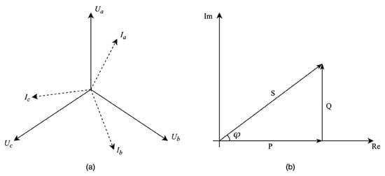
Figure 1.
The principle of power metering. (a) The relationship between voltages and currents for three-phase four-wire. (b) The relationship between active power, apparent power, and reactive power for single phase.
The corresponding three-phase total active power is calculated as follows, where cosφ denotes the power factor of the corresponding phase and φA is the angle between VA and IA:
3.2. Description of Metering Anomaly
The types of metering anomalies are diverse and vary slightly depending on the application scenario [1,42]. Ref. [43] categorized the types of anomalies into meter faults, power usage anomalies and transformer faults according to the location where the anomaly occurs. Ref. [44] categorized the types of anomalies into hardware faults, electricity anomalies and data anomalies according to hardware devices and electrical parameters. Ref. [9] analyzed the types of anomalies from the level of electricity consumption. We summarize the anomaly types by analyzing the abnormal SM data as follows:
(1) Loss of Voltage (LV): The current of a phase line is greater than the starting current set by the meter, but the voltage is lower than a critical voltage, and lasts for a period of time.
(2) Loss of Current (LC): Three-phase voltage is greater than the critical voltage, three-phase current in any phase is less than the starting current, and the other phases of the line load current is normal.
(3) Current Unbalance (CU): This mainly manifested in the three-phase when the current imbalance is too large, affecting the metering accuracy of the meter. Among them, the three-phase current unbalance is defined as follows [9]:
(4) Voltage Unbalance (VU): This means over or under voltage. The magnitude of the three-phase voltage exceeds the critical voltage, but there is a variation in the magnitude of one of the phases, leading to an imbalance in the three-phase voltage. The definition of three-phase voltage unbalance is as follows [9]:
(5) False Connection (FC): This includes: (a) Phase Disorder occurs when the currents are paired with incorrect voltages. (b) Phase Inversion happens when the phase of the voltage or current is directly reversed. This results in a change in the phase difference between voltage and current from φ to (π − φ). Consequently, the smart meter will detect a negative active power on that line and a reduced total active power [9].
(6) Factor Fault (FF): This indicates that there is a significant phase difference between the voltage and current. Typically, it is expected that the power factor in the substation should be close to one.
Although there are clear definitions for each type of abnormality, in practice it is not possible to accurately determine whether a section of SM data is normal or abnormal, and which specific type of abnormality it is based on these definitions. There are two main reasons for this:
- SM data can be interfered with by external noise when measuring the relevant electrical parameters, resulting in abnormal data.
- The data of a specific working condition are more similar to some of the abnormalities, such as current imbalance.
Therefore, it must be analyzed comprehensively from the physical relationship between the electrical parameters, as well as the change rule in time, otherwise it is easy to lead to misjudgment.
4. Method
In this paper, the metering anomaly diagnosis model is set up using the SM data shown in Table 1. X is a collection of time series of length T, denoted as X = {Xit=1,…,T | i = 1, …, N}, Xi∈RC×T. C is the number of variables. In particular, C equals 14; refer to Table 1. Y = {Yi|i = 1, …, N} are the corresponding labels. The unit of t is 15 min.

Table 1.
Electrical magnitudes of three-phase four-wire.
4.1. Framework
The overall architecture of the FSMAD model proposed in this article is presented in Figure 2. It consists of four components: Fault Data Injection (FDI) model, Variable Relation Network (VRN), Multi-Receptive Convolution Network (MRCNet), and MetricNet. Firstly, FSMAD employs the FDI model to manipulate the regular data and simulate the anomaly to train the neural networks. Secondly, VRN offers a learnable nonlinear transformation to extract the inherent correlation among variables in SM data. Meanwhile, the MRCNet utilizes convolution networks that incorporate multi-scale receptive fields to effectively capture temporal patterns. The diagnosis of the metering anomaly is ultimately accomplished through measuring the “distance” between pairs of features using a metric network. Further, we define whether two samples that are from the same class as a binary classification problem.
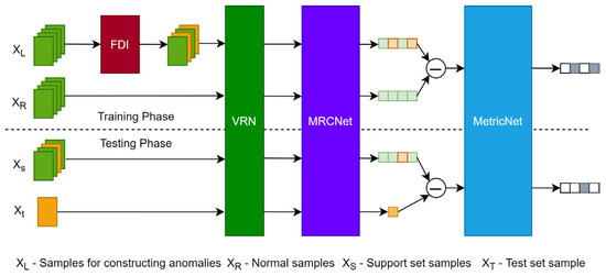
Figure 2.
The framework of FSMAD.
In the training phase, FSMAD only requires normal samples and splits into two equal parts: XL and XR. The part samples of XL are selected randomly and feed to the FDI module to simulate abnormal samples. All of the XR are kept normal. Then, FL and FR form the feature pairs, which is determined via MetricNet to be of the same class. In the testing phase, one sample from each category is randomly selected to form the support set, which is compared with the test sample, and the most similar support sample is output as the diagnosis result.
The FSMAD framework offers several advantages. (1) The model can be trained without any real anomaly samples. (2) The model is independent of domain knowledge. (3) The framework focuses on accurately comparing samples rather than understanding the anomalies themselves. This enables case-driven diagnosis and makes single-sample anomaly diagnosis possible. Finally, benefiting from the loose coupling among modules within FSMAD, the proposed framework can integrate any other time series network as the feature extractor.
4.2. FDI Model
In practice, cases of metering anomalies are very rare in smart grids. Therefore, in order to optimize diagnosis model, the mainstream approach is to construct simulated datasets [45,46]. In the CV or NLP, data augmentation [47,48] is another way to address this issue. In the field of time series, some researchers have also proposed corresponding data augment methods [49]. However, these methods are not suitable for metering anomaly diagnosis because they do not generate anomaly data that aligns with the principles of power metering. Therefore, we refer to the literature [45,46] and design a set of FDI models to generate metering anomaly data based on the principle of electricity measurement.
Any fault in the power metering process will lead to partial or total metering anomalies in the SM data, and the phenomena observed at the data level will follow the description in Section 3.2. Therefore, we propose the FDI model based on the relevant definitions as shown in Equation (5) and Table 2.
where, ph is randomly chosen from three-phase (A,B,C), abs() represents the absolute function, and t is time stamp. α(t), β(t), and γ(t) are random series which correspond to various FDIs. Their definitions refer to a certain FDI, which are provided in Table 2.
Table 2.
The definition of FDI model.
It is worth noting that the samples generated using the FDI model are only utilized for model training purposes in this paper.
4.3. Variable Relation Network
Currently, a prevalent approach to applying deep learning to industrial anomaly diagnosis involves integrating domain knowledge into the design and training of neural networks. However, the SM data contains 14 variables, which makes it challenging to develop effective data transformations based on domain knowledge. The transformations described in [9,10] still rely on the expertise of human experts. The generalization performance is limited in small sample situations. Therefore, this paper proposes a variable relationship network, as shown in Figure 3. It employs a data-driven approach to reveal the inherent relationships among variables and helps the feature network extract the optimal features.
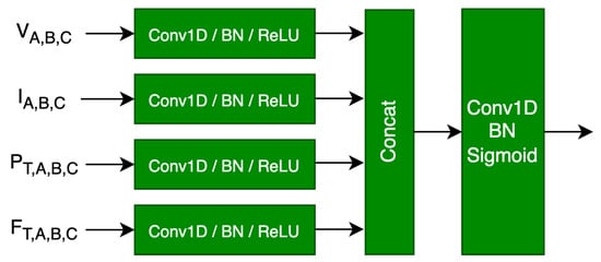
Figure 3.
The architecture of VRN.
Figure 3 illustrates the variable relationship network, which comprises a two-stage convolution. The first phase consists of four concurrent convolutional modules that process four primary categories of data: voltage, current, power, and power factor. Every convolution module comprises a one-dimensional convolutional layer, Batch Normalization (BN), and a ReLU activation layer. The convolution kernel size is 1, and the number of filters is 32. The outputs of the four convolution modules are then concatenated along the channel. The second stage of VRN consists of a one-dimensional convolutional layer, BN, and a sigmoid activation layer with a convolutional kernel size of 1 and 64 filters.
For VRN, the input is and the specific processing flow is as follows:
where XV, XI, XP, and XF represent voltage, current, power and power factor in the input SM data, respectively.
4.4. Multi-Receptive Convolution Network
The Multi-Receptive Convolution Network (MRCNet) analyzes the samples in the time domain and extracts their temporal features. The network structure of the MRCNet is illustrated in the left part of Figure 4. It consists of three convolutional modules and a Fully Connected layer (FC). Each convolution module comprises a one-dimensional convolution layer, a BN layer, a ReLU activation layer, and a max pooling layer. Specifically, the number of filters of each convolution layer is 64. The max pooling layer has a kernel size of 2.
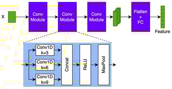
Figure 4.
The architecture of MRCNet.
The lth convolution module of the MRCNet takes an input . The specific processing flow is shown as follows:
where L represents the length of the input sequence of the lth convolution module, and d denotes the number of channels, .
Prior to producing feature vectors, the convolution module’s output is flattened through the utilization of a global average pooling layer. Afterwards, the feature vectors are transformed using a fully connected layer to make them sparser and improve their discriminability. In this case, the FC layer output dimension is 2048.
4.5. MetricNet
The MetricNet, as shown in the right part of Figure 4, consists of three consecutive fully connected layers that compute the similarity between the feature vectors of the support sample and the test sample. Before calculating the similarity, the support and test samples’ feature vectors are subtracted, and the absolute values of the differences are taken. With 512, 128, and 1 neuron, the three fully connected layers simulate a higher order “distance” function.
It is essentially a binary classification problem to determine whether the support and test samples belong to the same class. As a result, a sigmoid function is used to process the metric layer output, which represents the similarity between the support and test samples. The output of the sigmoid function is a probability value that falls within the range of 0 to 1. This probability indicates the likelihood that the sample pair belongs to the same class. The sigmoid output approaches 1 for samples that are highly similar and approaches 0 for samples that belong to different classes.
We use Binary Cross-Entropy loss (BCE) as the loss function for the FSMAD, specifically:
where yi represents the label of the ith feature pair, identifying whether the features of two samples are from the same category, 0 represents the same category, and 1 represents different categories. si is the “distance” between pairs of samples output by the metric layer, between 0 and 1.
4.6. Algorithm for Training
The key to model training is to ensure that the FSMAD acquires sufficient ability for comparison. However, as this paper has a limited number of real-world cases of metering anomalies, only the normal samples from the dataset are utilized during the training phase. The necessary anomaly samples are then generated using the FDI model.
The FSMAD is trained with Adam [50]. The training algorithm is presented by Algorithm 1. The key points of this algorithm are as follows:
- During training, a data batch will be split into two equal parts. In the first part, 50% of the samples will be randomly chosen to be manipulated as abnormal samples using the FDI model. The second part retains regular samples. The batch is composed of two parts that form sample pairs. Each pair is associated with a label, where 1 indicates the same class and 0 indicates a different class.
- The learning rate scheduling strategy involves reducing the rate by 50% after every 50 epochs.
- To mitigate overfitting, L2 regularization is applied to restrict the training process of the model using the specified parameter value of 5 × 10⁻⁴. It worth mentioning that we chose an empirical value of this parameter. In practice, it could be optimized by experiments.
| Algorithm 1 Mini-batch training of FSMAD |
| Require: = training inputs |
| Require: = labels for labeled inputs, fixed as 0 |
| Require: = false data injection model |
| Require: = VRN with trainable parameters |
| Require: = MRCNet with trainable parameters |
| Require: = MetricNet with trainable parameters |
|
5. Experiments and Results
5.1. Dataset
All data are extracted from a real AMI system. This dataset contains 504 three-phase four-wire smart meters, where there are 382 normal and 122 various abnormal meters that have been inspected in-field manually or labeled by a skillful expert. The duration of the data for each meter is 15 days, with a sampling interval of 15 min. We divided the samples by days, each containing 96 data points.
Some meters have missing data due to communication problems. The strategy for handling missing data was as follows: if a sample had less than five consecutive missing data points, we used the KNNImputer in Scikit-Learn [51] to input the missing values. However, if a sample has more than five consecutive missing data points, we found that the KNNImputer may recover incorrect data and therefore have to abandon the sample. Finally, we collect 7421 samples. Detailed information about the dataset is provided in Table 3.
Table 3.
Description of dataset.
The SM data used in this paper are the raw data collected via the smart meter; except for the voltage, the rest of the SM data are between 0 and 1, so we simply use the three-phase four-wire rated voltage (57.7 v) to normalize the voltage data.
5.2. Baseline
In this study, the FSMAD is evaluated against six baseline methods, encompassing both time series classification techniques and few-shot learning algorithms. It is important to note that all these methods are applied to preprocessed data to ensure a comprehensive and unbiased comparison.
- SVM: The kernel is set as the Radial Basis Function (RBF), and the penalty parameter is 0.01. Due to normal and abnormal imbalance, we give them proper weight according to the proportion of each category.
- XGBoost [52]: We set the number of trees to be 1000, the maximum depth of the tree to be 11, the weight of the smallest sub-node to be 10, and the learning rate to be 0.01.
- TCN [53]: is a generic architecture for time series modelling, based on dilated convolutional networks to model long-term dependencies of time series. We directly quote the official code and parameters.
- InceptionTime [54]: is a neural network model with a residual network architecture and three different sizes of receptive fields. We directly quote the official code and parameters.
- Siamese Network [27]: A shared network is used to extract the features of sample pairs, and the learnable L1 distance is used to judge whether the sample pairs are from the same class. We reproduce the method, mainly using 1D convolution instead of 2D convolution in the original paper, and the rest of the parameters are consistent with the paper.
- Relation Network [29]: Compared with the twin network, a more powerful relation network is used to evaluate whether the sample pairs are similar. We reproduce the method, mainly using one-dimensional convolution instead of the two-dimensional convolution in the original paper, and the rest of the parameters are consistent with the paper.
The SVM and XGBoost algorithms are implemented in the scikit-learn library [51]. The input features for the SVM and XGBoost models are generated through the utilization of Truncated Singular Value Decomposition (TruncatedSVD) on the sample data. The feature dimension was set to 32.
5.3. Evaluation Protocol and Metrics
5.3.1. Evaluation Protocol
For classification methods, we divided the data in Table 3 into equal proportions based on categories, with 30% allocated for training and 70% for testing.
For few-shot learning methods, we randomly select 2000 samples from the normal data for training and the rest for testing. The details are presented as follows:
- Training phase: Abnormal samples are simulated using the FDI model in 2000 normal samples.
- Test phase: One sample per class is randomly selected as a fixed support set, and the rest of the samples are all used as the test set.
5.3.2. Evaluation Metrics
We adopt the accuracy, AUC (Area Under ROC Curve) and F1 score as evaluation metrics. The results of all experiments are averaged from three independent trials using different random seeds.
Firstly, the diagnosis of metering anomalies can be considered as a multi-class classification problem. Hence, in this paper, we employ classification accuracy as a basic metric to evaluate the model’s performance.
Secondly, due to the imbalance of categories in the dataset, we also use AUC (Area Under ROC Curve) to evaluate the performance of the model. The AUC represents the relationship between the false positive rate and the true positive rate.
Lastly, we use the F1 score to comprehensively evaluate the model’s precision and recall. The F1 score is the harmonic mean of them. It thus symmetrically represents both precision and recall in one metric.
Finally, the F1 score is utilized to comprehensively evaluate the model’s capability in distinguishing between positive and negative samples. The F1 score represents the balanced combination of precision and recall. It represents both precision and recall in one metric in a balanced manner.
In this paper, we employed Scikit-Learn [54] to calculate above metrics.
5.4. Results and Discussion
FSMAD outperforms other baseline methods in all three metrics (as depicted in Figure 5) and the specific results can be found in Table 4. Benefiting from the physical dependence learning mechanism between the variables of the SM data, FSMAD demonstrates exceptional comparative performance even with zero abnormal cases in the training stage.
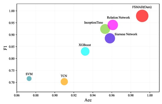
Figure 5.
Model performance comparison (The horizontal coordinates of the circle in the figure are Acc, the vertical coordinates are F1, and the diameter of the circle is the AUC of the model).
Table 4.
Performance comparison of our proposed FSMAD and baseline methods.
5.4.1. Main Results
The detailed performance of FSMAD and other baseline models is presented in Table 4. From the results in the table, it clearly demonstrates that the FSMAD proposed in this paper achieves outstanding results in the three metrics of Acc, AUC, and F1. The classification accuracy exhibits a notable enhancement of 3.1% when compared to the highest-performing relation network. The comparison results demonstrate the efficacy of VRN and more complex metric networks. Furthermore, it has been proven that the FDI-based electrical anomaly data improvement approach may effectively resolve the problem of insufficient anomaly situations.
The confusion matrix shown in Figure 6 further demonstrates that FSMAD uses contrastive learning to solve the category imbalance problem well and does not show any significant degradation in performance for categories with fewer samples in the test.
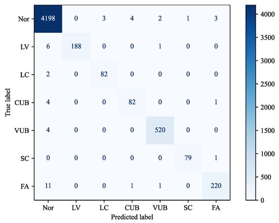
Figure 6.
Confusion matrix of FSMAD.
5.4.2. Component Study
(1) Performance of modules
As stated in Section 4, FSMAD uses the VRN and MetricNet to enhance the model’s feature extraction and comparison capabilities. In order to verify the effect of each module, this experiment utilizes the full FSMAD as a baseline, removes the modules one by one, and compares their performance. The specific experimental results are shown in Figure 7. As VRN and MetricNet are gradually removed, all three metrics degrade synchronously and significantly. Specifically, after all the previously described modules are removed, the performance of FSMAD declines to the same level as the Siamese Network.
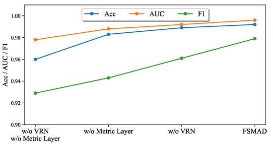
Figure 7.
Performance of FSMAF modules.
(2) Study of VRN
To analyze the performance of the VRN, we verify its effectiveness in improving the diagnosis of power metering anomalies by comparing the performance before and after the addition of a VRN, based on four deep learning-based baseline models. The results in Table 5 show that the performance of all four baseline models significantly improved by adding the VRN. In particular, the accuracy increased from 2.0% to 6.5%, respectively.
Table 5.
Performance of VRN.
In addition, we employed t-SNE [55] to visualize both the raw meter data and the features extracted using FSMAD, as shown in Figure 8. In Figure 8a, the t-SNE exhibit of the raw SM data demonstrates a complete overlap between the normal and abnormal category samples, which indicates very poor separability. Figure 8b illustrates the separability of the features extracted using FSMAD without VRN. The separability of the samples has markedly enhanced in comparison to the raw data. However, there are still some samples that overlapped, particularly those marked by the blue boxes in Figure 8b. Figure 8c illustrates the distinctiveness of the features obtained using full FSMAD. It can be noticed that almost all samples are clearly distinguishable. By comparing Figure 8b,c, the efficacy of the VRN is clearly demonstrated.
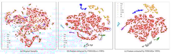
Figure 8.
t-SNE visualization of original samples and features extracted using FSMAD. (w means with, w/o means without).
Additionally, we conducted a comparison between the VRN and the domain knowledge-based data transformations mentioned in [11] utilizing a Siamese Network. Table 6 clearly demonstrates that applying domain knowledge to guide data transformation can significantly enhance the diagnostic performance of the Siamese Network. However, it still trails behind the effect of VRN in general. The primary rationale behind this is that VRN has the ability to construct a more comprehensive and precise correlation between data variables compared to conventional domain knowledge, thus enabling a more efficient approach to data transformation.
Table 6.
Comparing VRN with conventional domain knowledge.
(3) Study of MetricNet
To validate the enhanced FSMAD comparison capability of MetricNet, we conducted a comparison of the diagnostic performance for metering anomalies using one to four layers of MLPs and cosine distances. The results shown in Table 7 demonstrate that deeper MetricNet generally leads to better performance. However, once MetricNet reaches four layers of MLPs, a slight performance decline begins to occur. The three-layer MLP structure of MetricNet, as utilized in this paper, is deemed to be the optimal design.
Table 7.
Comparison of various metric approaches.
5.4.3. Parameter Study
(1) Number of training samples
Figure 9 presents the classification performance of FSMAD with different numbers of training samples. As can be seen from the results in the figure, the FSMAD proposed in this paper is still able to achieve 96% accuracy even with 500 samples. As the number of training samples increases, all three metrics improve rapidly, particularly AUC and F1. When the number of samples reaches 2000, the performance no longer shows significant improvement. However, in practical applications, we believe that having more training samples is helpful in improving the generalization performance of FSMAD.
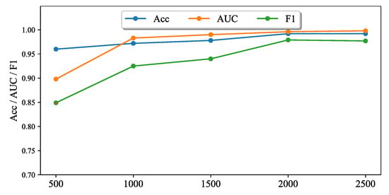
Figure 9.
Effect of number of training samples.
(2) Number of shots
All previous information about the performance of FSMAD is based on the one-shot task. In Table 8, we further present experimental results for the 5-shot, 10-shot, and 20-shot scenarios. As the number of shots increases, the improvement in the Acc, AUC, and F1 score is limited. Compared to the one-shot task, the 20-shot task achieved improvements of 0.2%, 0.1%, and 0.4% in the Acc, AUC and F1 score, respectively. It indicates that FSMAD exhibits a very strong ability for few-shot learning and generalization performance.
Table 8.
Effect of number of shots.
5.4.4. Convergence Analysis
In the FSMAD model, the epoch serves as a parameter that regulates the number of training iterations. In our experimental setup, an epoch is operationally defined as a single forward pass and backward pass comprising 1000 iterations. Consistent with the primary experiment, we maintained similar configurations. The investigation involved manipulating epoch values within the range of 0 to 100, with an incremental step size of 1. Figure 10 presents the results in terms of accuracy and training loss. It can be seen that as the epoch value increases, the training loss decreases, and the accuracy increases quickly. However, beyond a certain threshold, both the training loss and accuracy gradually converge. Throughout the entire training stage, the FSMAD does not experience overfitting. Nevertheless, it is observed that additional epochs do not yield further enhancements in performance.
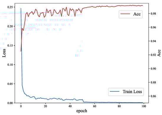
Figure 10.
Convergence Analysis.
6. Conclusions
Massively deployed smart meters are not only essential for power metering but are also gradually becoming important sensors for monitoring the power grid. Therefore, analyzing power metering data has become an important trend in smart grid. To address the problems of insufficient and unbalanced metering anomaly cases, this paper concentrates on diagnosing metering anomalies using few-shot learning. Firstly, we propose a multivariate time series few-shot learning framework and design a method to learn the physical dependencies among data variables. It leads to freedom from the domain knowledge. Second, a set of fault data injection models for smart meter data is established. It allows our FSMAD to be trained without any real-world anomaly cases. Finally, we conducted a large number of experiments using real-world smart meter data. The results demonstrate that our framework identified metering anomaly effectively and outperformed state-of-the-art methods by a significant margin. In the future, we would like to explore the detection and diagnosis of unknown anomalies and improve the model’s ability to adapt to new scenarios.
Author Contributions
Conceptualization, J.S. and F.W.; methodology, J.S. and C.W.; validation, W.Z. and P.G.; resources, X.D.; writing—original draft preparation, J.S. and C.W.; writing—review and editing, F.W.; supervision, J.S. All authors have read and agreed to the published version of the manuscript.
Funding
This research was funded by State Grid Zhejiang Marketing Service Center and Technology Project: Research on Key Technologies of on-line monitoring and anomaly recognition of the electric energy metering device (grant number: 5211YF230002).
Data Availability Statement
Data are contained within the article.
Conflicts of Interest
The authors declare no conflicts of interest.
References
- Elbouchikhi, E.; Zia, M.F.; Benbouzid, M.; El Hani, S. Overview of Signal Processing and Machine Learning for Smart Grid Condition Monitoring. Electronics 2021, 10, 2725. [Google Scholar] [CrossRef]
- He, J.; Luo, G.; Cheng, M.; Liu, Y.; Tan, Y.; Li, M. Small Sample Smart Substation Power Equipment Component Detection Based on Deep Transfer Learning. Proc. CSEE 2020, 40, 5506–5519. [Google Scholar] [CrossRef]
- Mohassel, R.; Fung, A.; Mohammadi, F.; Raahemifar, K. A survey on Advanced Metering Infrastructure. Int. J. Electr. Power Energy Syst. 2014, 63, 473–484. [Google Scholar] [CrossRef]
- Xue, Z.; Sun, Y.; Dong, Z.C.; Fang, Y.J. Fault diagnosis method of power consumption information acquisition system based on fuzzy Petri nets. Electr. Meas. Instrum. 2019, 56, 64–69. [Google Scholar]
- Wang, Y.; Chen, Q.; Hong, T.; Kang, C. Review of smart meter data analytics: Applications, methodologies, and challenges. IEEE Trans. Smart Grid 2019, 10, 3125–3148. [Google Scholar] [CrossRef]
- Cook, A.; Mısırlı, G.; Fan, Z. Anomaly Detection for IoT Time-Series Data: A Survey. IEEE Internet Things J. 2020, 7, 6481–6494. [Google Scholar] [CrossRef]
- Luo, G.; Yao, C.; Liu, Y.; Tan, Y.; He, J. Entropy SVM–Based Recognition of Transient Surges in HVDC Transmissions. Entropy 2018, 20, 421. [Google Scholar] [CrossRef]
- Guo, M.; Yang, N.; Chen, W. Deep-learningbased fault classification using Hilbert-Huang transform and convolutional neural network in power distribution systems. IEEE Sens. J. 2019, 19, 6905–6913. [Google Scholar] [CrossRef]
- Lu, X.; Zhou, Y.; Wang, Z.; Yi, Y.; Feng, L.; Wang, F. Knowledge Embedded Semi-Supervised Deep Learning for Detecting Non-Technical Losses in the Smart Grid. Energies 2019, 12, 3452. [Google Scholar] [CrossRef]
- Li, J.; Wang, F. Non-Technical Loss Detection in Power Grids with Statistical Profile Images Based on Semi-Supervised Learning. Sensors 2020, 20, 236. [Google Scholar] [CrossRef]
- Pandit, M. Expert system-a review article. Int. J. Eng. Sci. Res. Technol. 2013, 2, 1583–1585. [Google Scholar]
- Yang, J.; Xin, M.; Ou, J.; Wang, J.; Song, Q. Automatic diagnosis and rapid location of abnormal metering point of substation based on metrological automation system. Power Syst. Big Data 2017, 20, 68–71. [Google Scholar] [CrossRef]
- Jiang, X.; Wang, D.; Ning, Y.; Zhang, C. Query Method for Optimal Diagnosis of Power System Faults. High Volt. Eng. 2017, 43, 1311–1316. [Google Scholar] [CrossRef]
- Zhou, J.; Wu, Z.; Wang, Q.; Yu, Z. Fault Diagnosis Method of Smart Meters Based on DBN-CapsNet. Electronics 2022, 11, 1603. [Google Scholar] [CrossRef]
- Wu, R.; Zhang, A.; Tian, X.; Zhang, T. Anomaly detection algorithm based on improved K-means for electric power data. J. East China Norm. Univ. (Nat. Sci.) 2020, 4, 79–87. [Google Scholar] [CrossRef]
- Zhou, F.; Cheng, Y.Y.; Du, J.; Feng, L.; Xiao, J.; Zhang, J.M. Construction of Multidimensional Electric Energy Meter Abnormal Diagnosis Model Based on Decision Tree Group. In Proceedings of the 2019 IEEE 8th Joint International Information Technology and Artificial Intelligence Conference (ITAIC), Chongqing, China, 24–26 May 2019; pp. 24–26. [Google Scholar]
- Coma-Puig, B.; Carmona, J.; Gavaldà, R.; Alcoverro, S.; Martin, V. Fraud detection in energy consumption: A supervised approach. In Proceedings of the IEEE International Conference on Data Science and Advanced Analytics (DSAA), Montreal, QC, Canada, 17–19 October 2016; pp. 120–129. [Google Scholar] [CrossRef]
- Schmidhuber, J. Deep learning in neural networks: An overview. Neural Netw. 2015, 61, 85–117. [Google Scholar] [CrossRef]
- LeCun, Y.; Bengio, Y.; Hinton, G. Deep learning. Nature 2015, 521, 436–444. [Google Scholar] [CrossRef]
- Wen, L.; Li, X.; Gao, L.; Zhang, Y. A New Convolutional Neural Network-Based Data-Driven Fault Diagnosis Method. IEEE Trans. Ind. Electron 2018, 65, 5990–5998. [Google Scholar] [CrossRef]
- Shao, H.; Jiang, H.; Lin, Y.; Li, X. A novel method for intelligent fault diagnosis of rolling bearings using ensemble deep auto-encoders. Mech. Syst. Signal Process. 2018, 102, 278–297. [Google Scholar] [CrossRef]
- Wu, N.; Wang, Z. Bearing Fault Diagnosis Based on the Combination of One-Dimensional CNN and Bi-LSTM. Modul. Mach. Tool Autom. Manuf. Tech. 2021, 571, 38–41. [Google Scholar] [CrossRef]
- Ren, B.; Zheng, Y.; Wang, Y.; Sheng, S.; Li, J.; Zhang, H.; Zheng, C. Fault Location of Secondary Equipment in Smart Substation Based on Deep Learning. Power Syst. Technol. 2021, 45, 713–721. [Google Scholar] [CrossRef]
- Morais, J.; Pires, Y.; Cardoso, C.; Klautau, A. A framework for evaluating automatic classification of underlying causes of disturbances and its application to short-circuit faults. IEEE Trans. Power Deliv. 2010, 25, 2083–2094. [Google Scholar] [CrossRef]
- Kou, Y.; Cui, G.; Fan, J.; Chen, X.; Li, W. Machine learning based models for fault detection in automatic meter reading systems. In Proceedings of the 2017 International Conference on Security, Pattern Analysis, and Cybernetics (SPAC), Shenzhen, China, 15–17 December 2017; pp. 684–689. [Google Scholar] [CrossRef]
- Li, F.; Fergus, R.; Perona, P. One-shot learning of object categories. IEEE Trans. Pattern Anal. Mach. Intell. 2006, 28, 594–611. [Google Scholar]
- Koch, G.; Zemel, R.; Salakhutdinov, R. Siamese neural networks for one-shot image recognition. In Proceedings of the 32nd International Conference on Machine Learning, Lille, France, 6–11 July 2015; Volume 2. [Google Scholar]
- Vinyals, O.; Blundell, C.; Lillicrap, T.; Wierstra, D. Matching networks for one shot learning. In Advances in Neural Information Processing Systems; MIT Press: Cambridge, MA, USA, 2016; pp. 3630–3638. [Google Scholar]
- Sung, F.; Yang, Y.; Zhang, L.; Xiang, T.; Torr, P.H.; Hospedales, T.M. Learning to compare: Relation network for few-shot learning. In Proceedings of the IEEE Conference on Computer Vision and Pattern Recognition, Salt Lake City, UT, USA, 18–23 June 2018; pp. 1199–1208. [Google Scholar]
- Snell, J.; Swersky, K.; Zemel, R. Prototypical networks for few-shot learning. In Advances in Neural Information Processing Systems; MIT Press: Cambridge, MA, USA, 2017; Volume 30. [Google Scholar]
- Sumit, C.; Hadsell, R.; LeCun, Y. Learning a similarity metric discriminatively, with application to face verification. In Proceedings of the 2005 IEEE Computer Society Conference on Computer Vision and Pattern Recognition (CVPR’05), San Diego, CA, USA, 20–25 June 2005. [Google Scholar]
- Schroff, F.; Kalenichenko, D.; Philbin, J. Facenet: A unified embedding for face recognition and clustering. In Proceedings of the IEEE Conference on Computer Vision and Pattern Recognition, Boston, MA, USA, 7–12 June 2015; pp. 815–823. [Google Scholar]
- Wang, Y.X.; Hebert, M. Learning from small sample sets by combining unsupervised meta-training with CNNs. In Advances in Neural Information Processing Systems; MIT Press: Cambridge, MA, USA, 2016; pp. 244–252. [Google Scholar]
- Vilalta, R.; Drissi, Y. A perspective view and survey of meta-learning. Artif. Intell. Rev. 2002, 18, 77–95. [Google Scholar] [CrossRef]
- Rajendran, J.; Irpan, A.; Jang, E. Meta-learning requires meta-augmentation. Adv. Neural Inf. Process. Syst. 2020, 33, 5705–5715. [Google Scholar]
- Finn, C.; Abbeel, P.; Levine, S. Model-agnostic meta-learning for fast adaptation of deep networks. Int. Conf. Mach. Learn. 2017, 70, 1126–1135. [Google Scholar]
- Ravi, S.; Larochelle, H. Optimization as a model for few-shot learning. In Proceedings of the International Conference on Learning Representations (ICLR), Toulon, France, 24–26 April 2017. [Google Scholar]
- Zhang, S.; Ye, F.; Wang, B.; Habetler, T.G. Few-shot bearing fault diagnosis based on model-agnostic meta-learning. IEEE Trans. Ind. Appl. 2021, 57, 4754–4764. [Google Scholar] [CrossRef]
- Wang, Y.; Yan, J.; Ye, X.; Jing, Q.; Wang, J.; Geng, Y. Few-Shot Transfer Learning With Attention Mechanism for High-Voltage Circuit Breaker Fault Diagnosis. IEEE Trans. Ind. Appl. 2022, 58, 3353–3360. [Google Scholar] [CrossRef]
- Yu, X.; Ju, X.; Wang, Y.; Qi, H. A metric learning network based on attention mechanism for Power grid defect identification. J. Phys. Conf. Ser. 2020, 1693, 012146. [Google Scholar] [CrossRef]
- Xue, L.; Jiang, A.; Zheng, X.; Qi, Y.; He, L.; Wang, Y. Few-Shot Fault Diagnosis Based on an Attention-Weighted Relation Network. Entropy 2024, 26, 22. [Google Scholar] [CrossRef]
- Akbar, S.; Vaimann, T.; Asad, B.; Kallaste, A.; Sardar, M.U.; Kudelina, K. State-of-the-Art Techniques for Fault Diagnosis in Electrical Machines: Advancements and Future Directions. Energies 2023, 16, 6345. [Google Scholar] [CrossRef]
- Fan, J.; Chen, X.; Zhou, Y. An Intelligent Analytical Method of Abnormal Metering Device Based on Power Consumption Information Collection System. Electr. Meas. Instrum. 2013, 50, 4–9. [Google Scholar]
- Wang, X.; Wu, Y.; Zhang, Y. Method of smart meter online monitoring based on data mining. Electr. Meas. Instrum. 2016, 53, 65–69. [Google Scholar]
- Jokar, P.; Arianpoo, N.; Leung, V.C.M. Electricity Theft Detection in AMI Using Customers’ Consumption Patterns. IEEE Trans. Smart Grid 2016, 7, 216–226. [Google Scholar] [CrossRef]
- Zanetti, M.; Jamhour, E.; Pellenz, M.; Penna, M.; Zambenedetti, V.; Chueiri, I. A Tunable Fraud Detection System for Advanced Metering Infrastructure Using Short-Lived Patterns. IEEE Trans. Smart Grid 2019, 10, 830–840. [Google Scholar] [CrossRef]
- Benaim, S.; Wolf, L. One-shot unsupervised cross domain translation. In Advances in Neural Information Processing Systems (NIPS); MIT Press: Cambridge, MA, USA, 2018; pp. 2104–2114. [Google Scholar]
- Zhang, Y.; Tang, H.; Jia, K. Fine-grained visual categorization using meta-learning optimization with sample selection of auxiliary data. In Proceeding of the 15th European Conference on European Conference on Computer Vision (ECCV), Munich, Germany, 8–14 September 2018; pp. 233–248. [Google Scholar]
- Wen, Q.; Sun, L.; Song, X.; Gao, J.; Wang, X.; Xu, H. Time Series Data Augmentation for Deep Learning: A Survey. In Proceeding of the Thirtieth International Joint Conference on Artificial Intelligence (IJCAI-21), Montreal, QC, Canada, 19–27 August 2021; pp. 4653–4660. [Google Scholar]
- Kingma, D.; Ba, J. Adam: A Method for Stochastic Optimization. arXiv 2014, arXiv:1412.6980. [Google Scholar]
- Pedregosa, F.; Varoquaux, G.; Gramfort, A.; Michel, V.; Thirion, B.; Grisel, O.; Blondel, M.; Prettenhofer, P.; Weiss, R.; Dubourg, V.; et al. Scikit-learn: Machine learning in Python. J. Mach. Learn. Res. 2011, 12, 2825–2830. [Google Scholar]
- Chen, T.; Guestrin, C. XGBoost: A Scalable Tree Boosting System. In Proceeding of the 22nd ACM SIGKDD Conference on Knowledge Discovery and Data Mining, San Francisco, CA, USA, 13–17 August 2016. [Google Scholar]
- Bai, S.; Kolter, J.Z.; Koltun, V. An Empirical Evaluation of Generic Convolutional and Recurrent Networks for Sequence Modeling. arXiv 2018, arXiv:1803.01271. [Google Scholar]
- Ismail Fawaz, H.; Lucas, B.; Forestier, G.; Pelletier, C.; Schmidt, D.F.; Weber, J.; Webb, G.I.; Idoumghar, L.; Muller, P.; Petitjean, F. InceptionTime: Finding AlexNet for time series classification. Data Min. Knowl. Discov. 2019, 34, 1936–1962. [Google Scholar] [CrossRef]
- Van der Maaten, L.; Hinton, G. Visualizing data using t-SNE. J. Mach. Learn. Res. 2008, 9, 2579–2605. [Google Scholar]
Disclaimer/Publisher’s Note: The statements, opinions and data contained in all publications are solely those of the individual author(s) and contributor(s) and not of MDPI and/or the editor(s). MDPI and/or the editor(s) disclaim responsibility for any injury to people or property resulting from any ideas, methods, instructions or products referred to in the content. |
© 2024 by the authors. Licensee MDPI, Basel, Switzerland. This article is an open access article distributed under the terms and conditions of the Creative Commons Attribution (CC BY) license (https://creativecommons.org/licenses/by/4.0/).