
Data-Driven Management Systems for Wave-Powered Renewable Energy Communities


Abstract
1. Introduction
- The implementation of the long short-term memory neural network (LSTM-NN) for energy forecasting, surpassing traditional persistence forecasting methods by capturing intricate temporal dependencies in the data, thus elevating energy prediction accuracy and reliability.
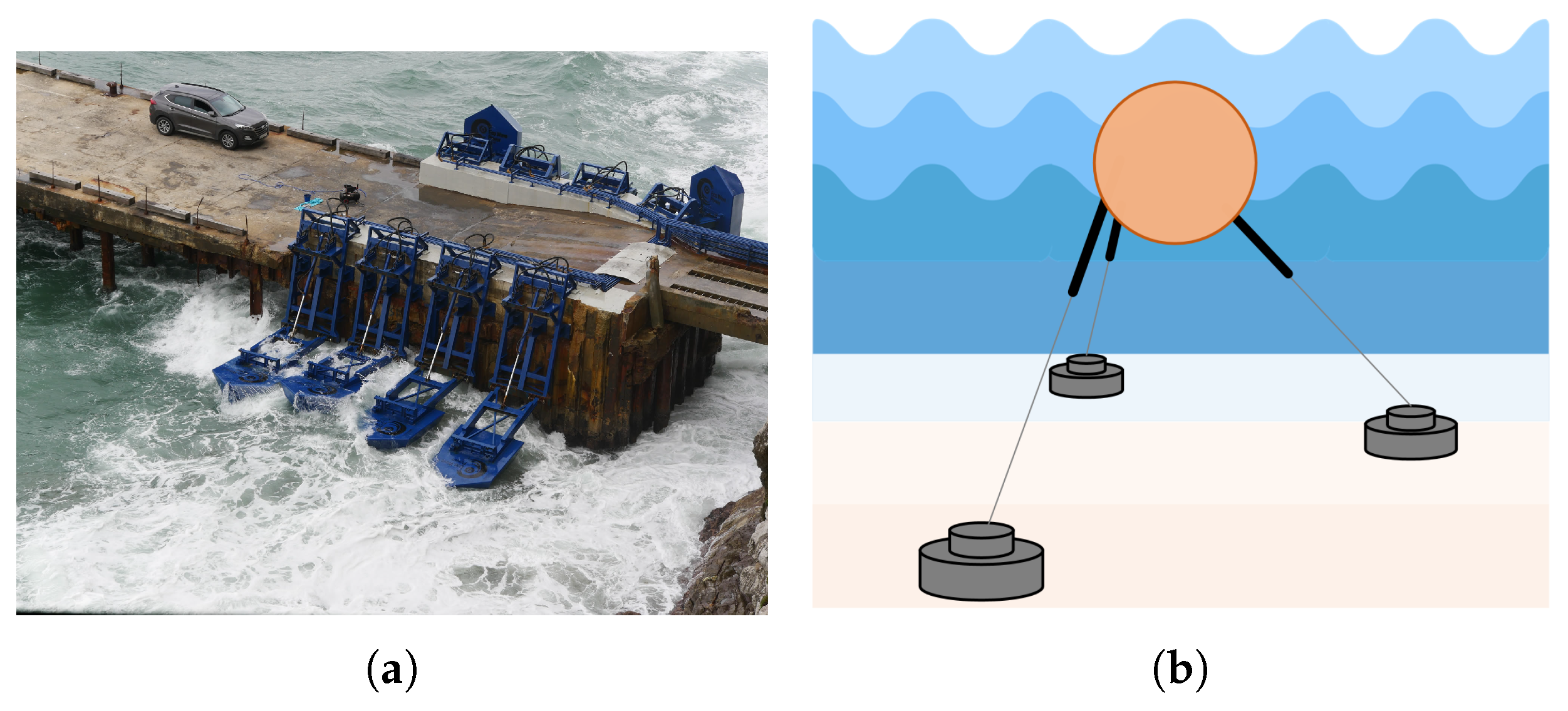
- Modification of a fully submerged three-tether buoy WEC hydrodynamic model, enabling real-time power output prediction using forecasted wave peak height, wave peak time period, and wave direction.
- Development of an intelligent REC EMS service that concurrently forecasts energy consumption, wave parameters, and WEC power output through a real-data-driven approach, while showcasing system versatility by functioning effectively even without an energy storage system (ESS), relying solely on super capacitor (SC) and WEC, illustrating its adaptability and resilience.
2. Long Short-Term Memory Neural Network
| Algorithm 1 Long short-term memory (LSTM). |
| Require: Time-Series Data |
| Ensure: RMSE of the forecasted data |
|
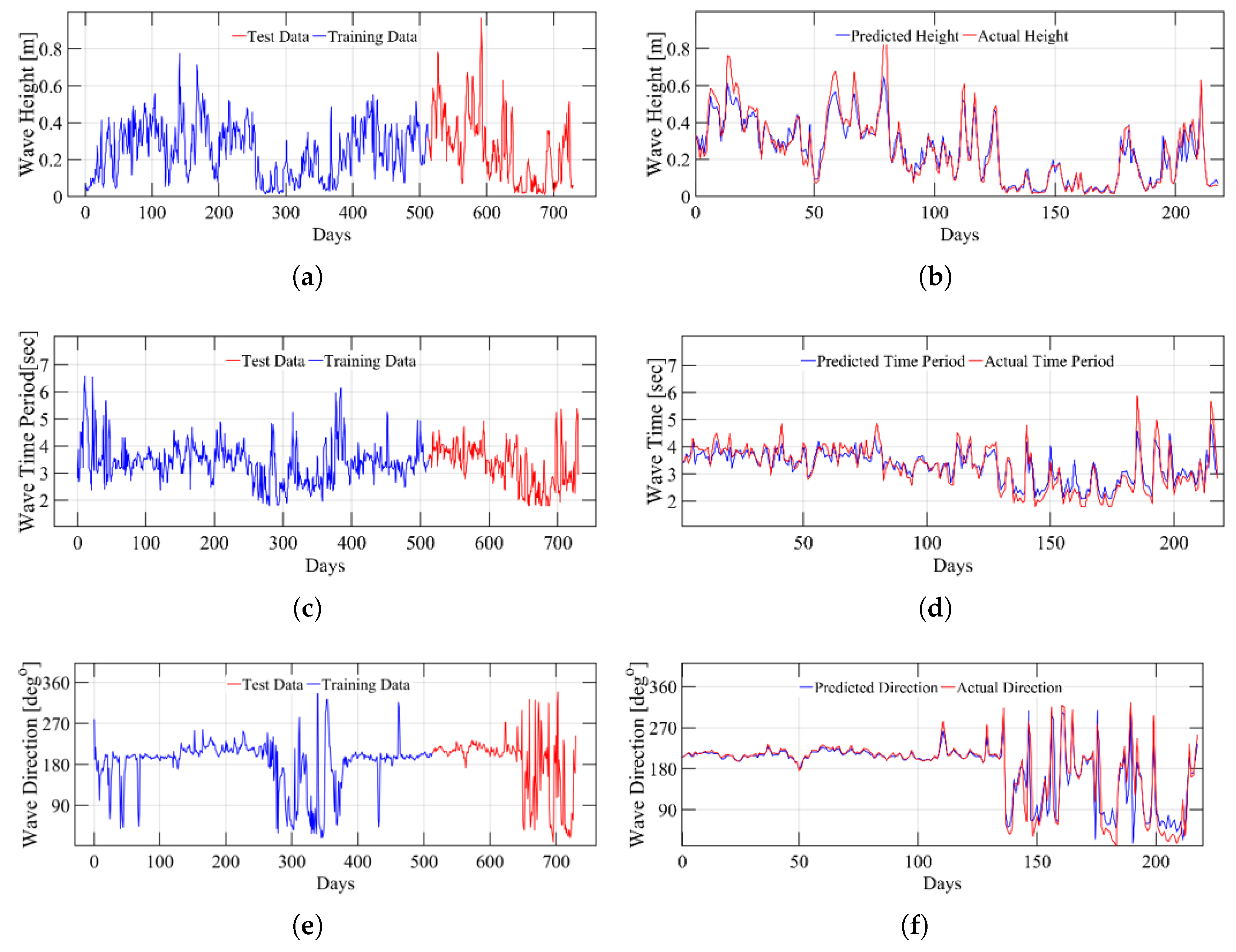
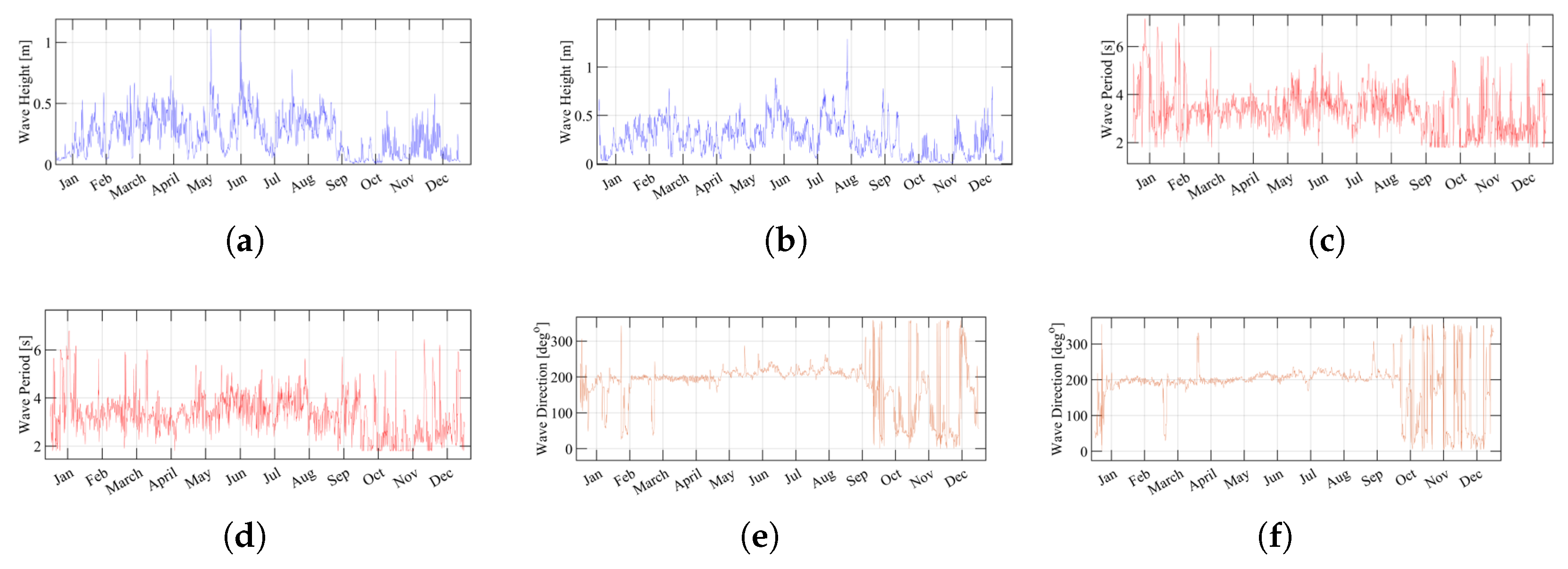
2.1. Model Training and Validation of Waves Data
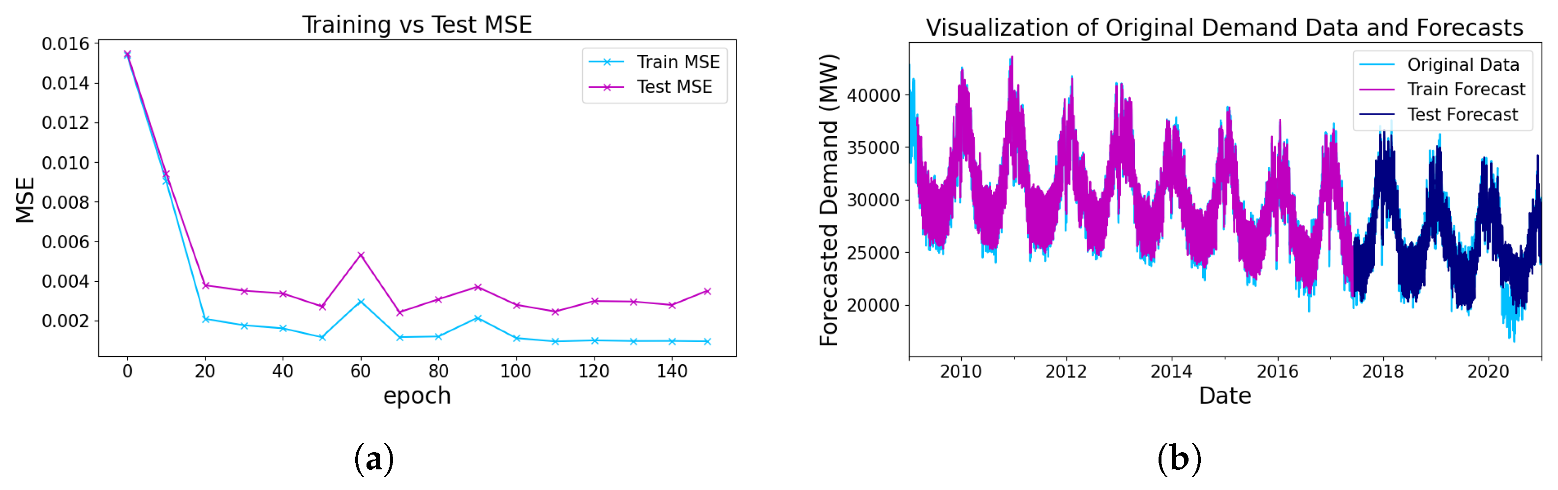
2.2. Model Training and Validation of Energy Consumption Data
2.2.1. Many to One Time-Series-Based Energy Demand Forecasting
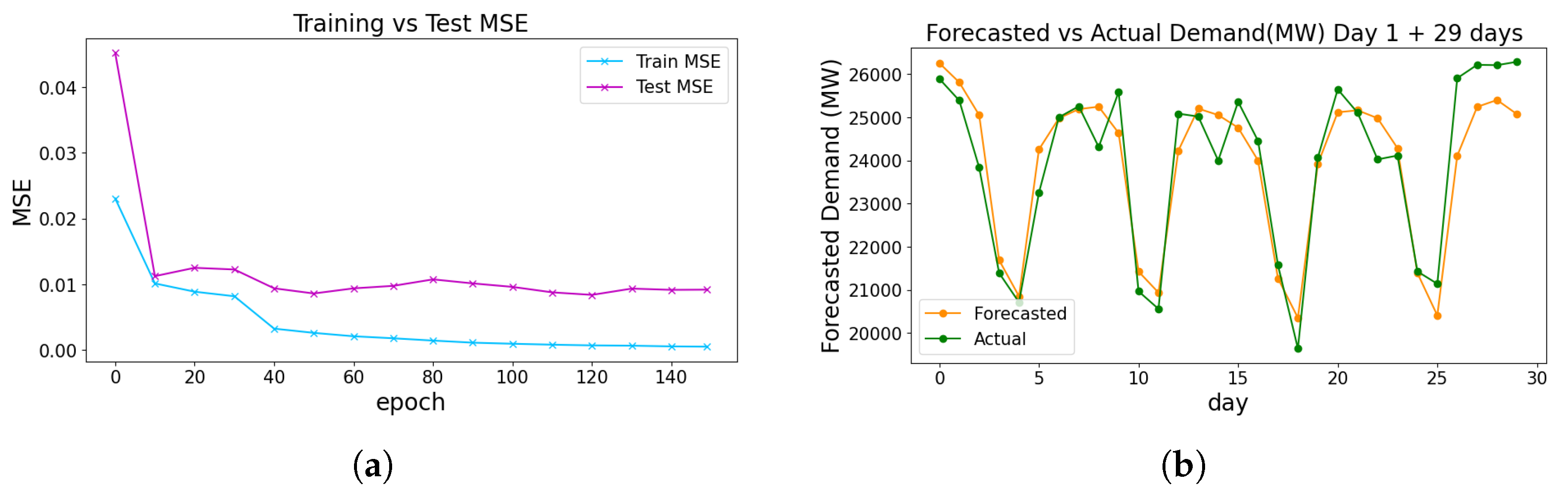
2.2.2. Many to Many Time-Series-Based Energy Demand Forecasting
3. Wave Energy Converter Power Calculation Model
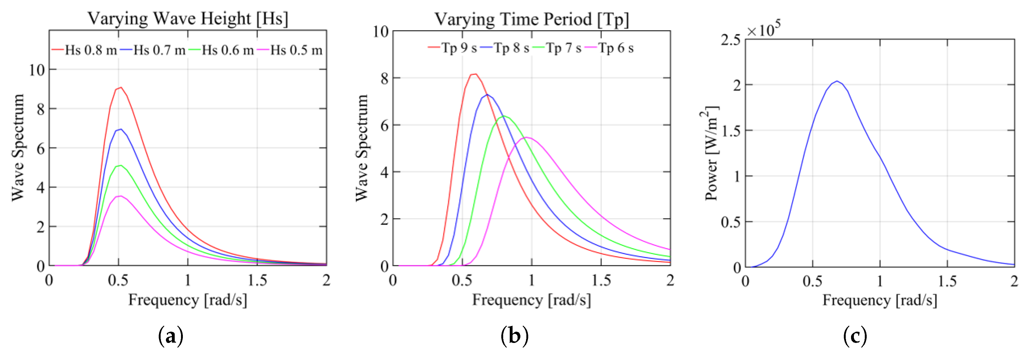
3.1. Wave Spectrum and Power Density
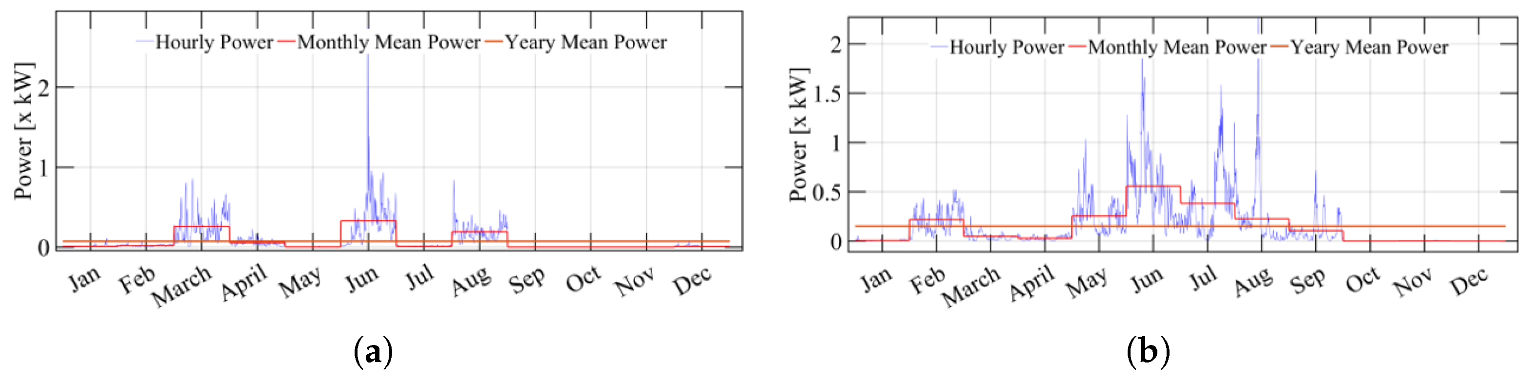
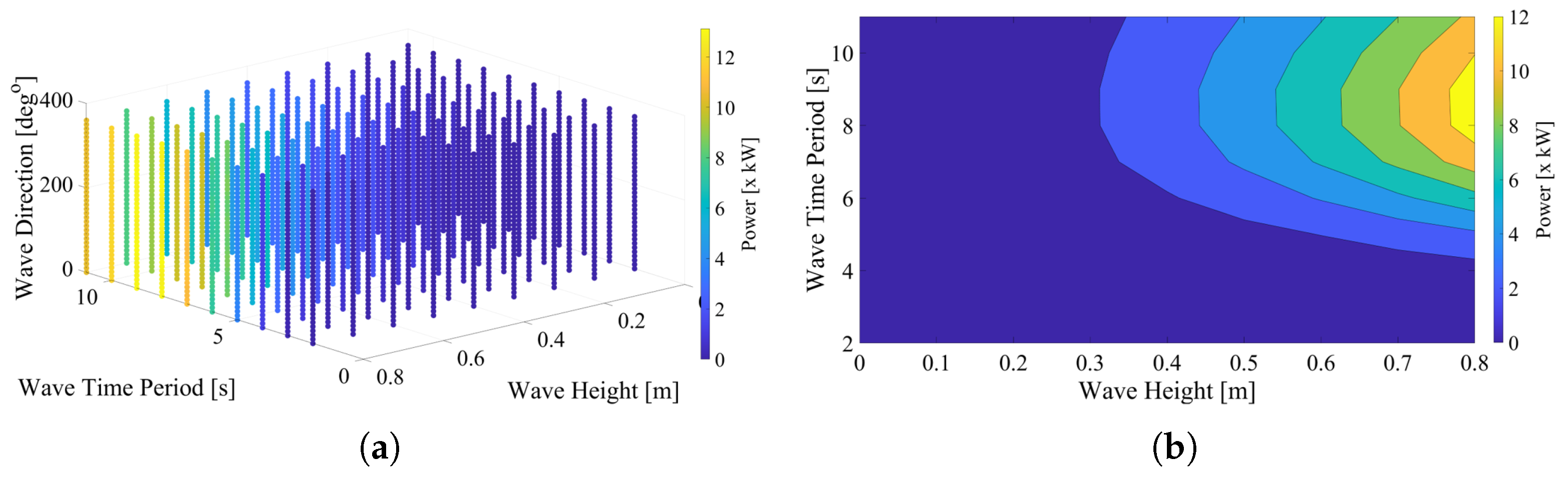
3.2. Power Array
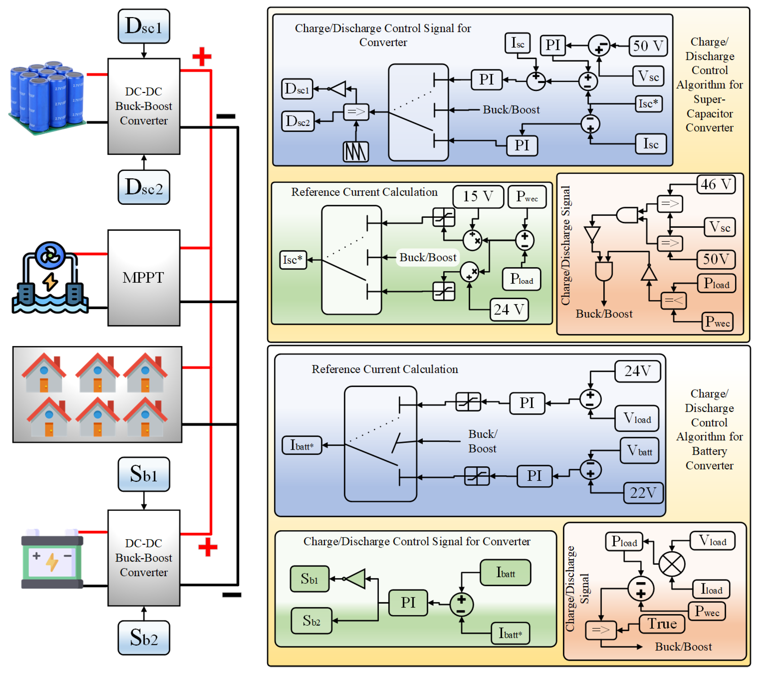
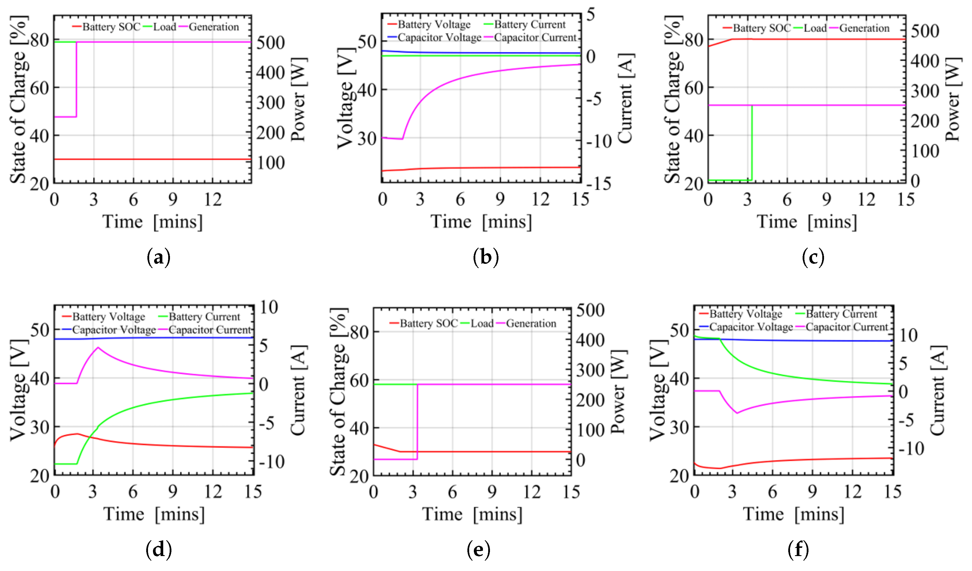
4. The Energy Management Strategy
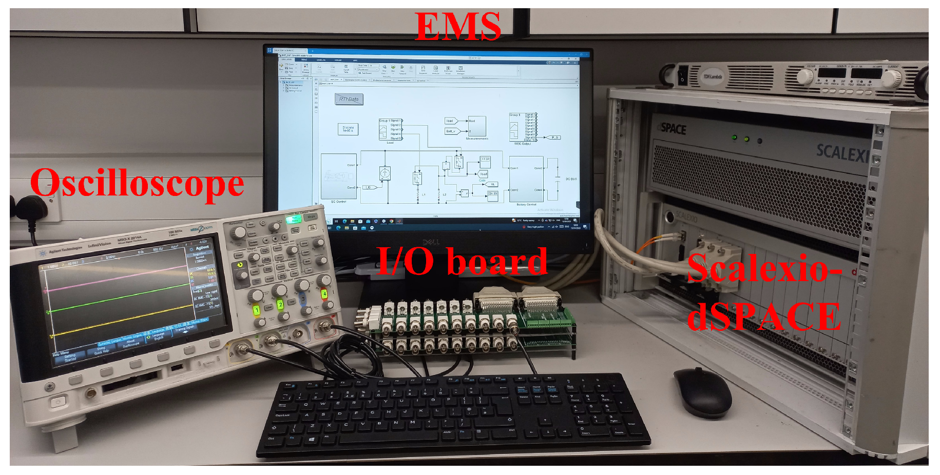
5. Case Study Specification
6. Experimental Results and Discussion
7. Conclusions
8. Future Work
Author Contributions
Funding
Institutional Review Board Statement
Informed Consent Statement
Data Availability Statement
Acknowledgments
Conflicts of Interest
Abbreviations
| ANN | artificial neural networks |
| ARIM | autoregressive integrated models |
| ARMAM | autoregressive moving average models |
| EMS | energy management system |
| ESS | energy storage system |
| EWMA | exponential weighted moving average |
| HIL | hardware-in-the-Loop |
| LCOE | levelised cost of energy |
| LSTM | long short-term memory |
| LSTM-NN | song short-term memory neural network |
| MSE | mean square error |
| ML | machine learning |
| ML-NN | multilayer neural network |
| MPPT | maximum power point tracking |
| NN | neural network |
| RBF | radial basis function |
| RB-NN | radial basis neural network |
| RECs | renewable energy communities |
| RES | renewable energy source |
| RMSE | root mean square error |
| R-NN | recurrent neural network |
| SC | super capacitor |
| SGP | system-generated power |
| SOC | state of charge |
| SSP | system-stored power |
| WEC | wave energy converter |
References
- Renewables 2021. IEA, 2021. Available online: https://www.iea.org/reports/renewables-2021 (accessed on 15 December 2022).
- Neshat, M.; Mirjalili, S.; Sergiienko, N.Y.; Esmaeilzadeh, S.; Amini, E.; Heydari, A.; Garcia, D.A. Layout optimisation of offshore wave energy converters using a novel multi-swarm cooperative algorithm with backtracking strategy: A case study from coasts of Australia. Energy 2022, 239, 122463. [Google Scholar] [CrossRef]
- Alirahmi, S.M.; Dabbagh, S.R.; Ahmadi, P.; Wongwises, S. Multi-objective design optimization of a multi-generation energy system based on geothermal and solar energy. Energy Convers. Manag. 2020, 205, 112426. [Google Scholar] [CrossRef]
- Neary, V.S.; Kobos, P.H.; Jenne, D.S.; Yu, Y.H. Levelized Cost of Energy for Marine Energy Conversion (Mec) Technologies; Technical Report; Sandia National Lab. (SNL-NM): Albuquerque, NM, USA, 2016. [Google Scholar]
- Kalogeri, C.; Galanis, G.; Spyrou, C.; Diamantis, D.; Baladima, F.; Koukoula, M.; Kallos, G. Assessing the European offshore wind and wave energy resource for combined exploitation. Renew. Energy 2017, 101, 244–264. [Google Scholar] [CrossRef]
- Fusco, F.; Nolan, G.; Ringwood, J.V. Variability reduction through optimal combination of wind/wave resources—An Irish case study. Energy 2010, 35, 314–325. [Google Scholar] [CrossRef]
- Point Absorber. Available online: https://www.oceansofenergy.blue/technology (accessed on 10 April 2023).
- Oscillating Water Column (OWC). Available online: https://www.ocean-energy-systems.org/technology/owc/ (accessed on 10 April 2023).
- Wave Energy-Attenuator. Available online: https://www.renewableuk.com/page/WaveEnergyAttenuator (accessed on 10 April 2023).
- World Intellectual Property Organization. Peniche, Portugal: Turning the Tide with Wave Energy. 2020. Available online: https://www.wipo.int/ip-outreach/en/ipday/2020/case-studies/peniche.html (accessed on 16 April 2023).
- Power, E.W. Eco Wave Power’s Gibraltar Wave Energy Power Station. 2023. Available online: https://www.ecowavepower.com/projects/gibraltar/ (accessed on 16 April 2023).
- Technology, P. Pelamis Wave Power’s Agucadoura Wave Farm, Portugal. 2023. Available online: https://www.power-technology.com/projects/pelamis (accessed on 16 April 2023).
- Offshore Energy. OE Buoy Arrives in Hawaii. 2020. Available online: https://www.offshore-energy.biz/oe-buoy-arrives-in-hawaii/ (accessed on 16 April 2023).
- Kumar, N.K.; Savitha, R.; Al Mamun, A. Regional ocean wave height prediction using sequential learning neural networks. Ocean Eng. 2017, 129, 605–612. [Google Scholar] [CrossRef]
- Law, Y.; Santo, H.; Lim, K.; Chan, E. Deterministic wave prediction for unidirectional sea-states in real-time using Artificial Neural Network. Ocean Eng. 2020, 195, 106722. [Google Scholar] [CrossRef]
- Abed-Elmdoust, A.; Kerachian, R. Wave height prediction using the rough set theory. Ocean Eng. 2012, 54, 244–250. [Google Scholar] [CrossRef]
- Ali, M.; Prasad, R. Significant wave height forecasting via an extreme learning machine model integrated with improved complete ensemble empirical mode decomposition. Renew. Sustain. Energy Rev. 2019, 104, 281–295. [Google Scholar] [CrossRef]
- Agrawal, J.; Deo, M. On-line wave prediction. Mar. Struct. 2002, 15, 57–74. [Google Scholar] [CrossRef]
- De Matos, J.G.; e Silva, F.S.; Ribeiro, L.A.d.S. Power control in AC isolated microgrids with renewable energy sources and energy storage systems. IEEE Trans. Ind. Electron. 2014, 62, 3490–3498. [Google Scholar] [CrossRef]
- Vasquez, J.C.; Guerrero, J.M.; Savaghebi, M.; Eloy-Garcia, J.; Teodorescu, R. Modeling, analysis, and design of stationary-reference-frame droop-controlled parallel three-phase voltage source inverters. IEEE Trans. Ind. Electron. 2012, 60, 1271–1280. [Google Scholar] [CrossRef]
- Elrayyah, A.; Cingoz, F.; Sozer, Y. Construction of nonlinear droop relations to optimize islanded microgrid operation. IEEE Trans. Ind. Appl. 2015, 51, 3404–3413. [Google Scholar] [CrossRef]
- Meng, L.; Sanseverino, E.R.; Luna, A.; Dragicevic, T.; Vasquez, J.C.; Guerrero, J.M. Microgrid supervisory controllers and energy management systems: A literature review. Renew. Sustain. Energy Rev. 2016, 60, 1263–1273. [Google Scholar] [CrossRef]
- Sui, Q.; Zhang, R.; Wu, C.; Wei, F.; Lin, X.; Li, Z. Stochastic scheduling of an electric vessel-based energy management system in pelagic clustering islands. Appl. Energy 2020, 259, 114155. [Google Scholar] [CrossRef]
- Teimourzadeh Baboli, P.; Shahparasti, M.; Parsa Moghaddam, M.; Haghifam, M.R.; Mohamadian, M. Energy management and operation modelling of hybrid AC–DC microgrid. Iet Gener. Transm. Distrib. 2014, 8, 1700–1711. [Google Scholar] [CrossRef]
- Kakigano, H.; Miura, Y.; Ise, T. Distribution voltage control for DC microgrids using fuzzy control and gain-scheduling technique. IEEE Trans. Power Electron. 2012, 28, 2246–2258. [Google Scholar] [CrossRef]
- Iqbal, S.; Mehran, K. A Day-Ahead Energy Management for Multi MicroGrid System to Optimize the Energy Storage Charge and Grid Dependency—A Comparative Analysis. Energies 2022, 15, 4062. [Google Scholar] [CrossRef]
- Olivares, D.E.; Cañizares, C.A.; Kazerani, M. A centralized energy management system for isolated microgrids. IEEE Trans. Smart Grid 2014, 5, 1864–1875. [Google Scholar] [CrossRef]
- Luna, A.C.; Meng, L.; Diaz, N.L.; Graells, M.; Vasquez, J.C.; Guerrero, J.M. Online energy management systems for microgrids: Experimental validation and assessment framework. IEEE Trans. Power Electron. 2017, 33, 2201–2215. [Google Scholar] [CrossRef]
- Malysz, P.; Sirouspour, S.; Emadi, A. An optimal energy storage control strategy for grid-connected microgrids. IEEE Trans. Smart Grid 2014, 5, 1785–1796. [Google Scholar] [CrossRef]
- Chen, Y.K.; Wu, Y.C.; Song, C.C.; Chen, Y.S. Design and implementation of energy management system with fuzzy control for DC microgrid systems. IEEE Trans. Power Electron. 2012, 28, 1563–1570. [Google Scholar] [CrossRef]
- Pamulapati, T.; Cavus, M.; Odigwe, I.; Allahham, A.; Walker, S.; Giaouris, D. A Review of Microgrid Energy Management Strategies from the Energy Trilemma Perspective. Energies 2022, 16, 289. [Google Scholar] [CrossRef]
- Tumeran, N.L.; Yusoff, S.H.; Gunawan, T.S.; Hanifah, M.S.A.; Zabidi, S.A.; Pranggono, B.; Yunus, M.S.F.M.; Sapihie, S.N.M.; Halbouni, A.H. Model Predictive Control Based Energy Management System Literature Assessment for RES Integration. Energies 2023, 16, 3362. [Google Scholar] [CrossRef]
- Peres, D.; Iuppa, C.; Cavallaro, L.; Cancelliere, A.; Foti, E. Significant wave height record extension by neural networks and reanalysis wind data. Ocean Model. 2015, 94, 128–140. [Google Scholar] [CrossRef]
- Durán-Rosal, A.M.; Hervás-Martínez, C.; Tallón-Ballesteros, A.J.; Martínez-Estudillo, A.; Salcedo-Sanz, S. Massive missing data reconstruction in ocean buoys with evolutionary product unit neural networks. Ocean Eng. 2016, 117, 292–301. [Google Scholar] [CrossRef]
- National Grid Electricity System Operator Data Library. Available online: https://www.nationalgrideso.com/data-library (accessed on 15 December 2022).
- Neshat, M.; Alexander, B.; Sergiienko, N.; Wagner, M. A new insight into the position optimization of wave energy converters by a hybrid local search. arXiv 2019, arXiv:1904.09599. [Google Scholar]
- Meta Ocean. Available online: http://https://metaoceanhub.com/ (accessed on 15 December 2022).


| Parameter | Value (Waves) | Value (Load) |
|---|---|---|
| Observation | 710 Days [n] | 60 Days [n] |
| Train Set | 70 [%] | 70 [%] |
| Test Set | 30 [%] | 30 [%] |
| LSTM Neurons | 128 [n] | 128 [n] |
| Batch Size | 32 [n] | 64 [n] |
| Epochs | 70 [n] | 150 [n] |
| Data Type | Persistence Forecast | LSTM Forecast | ||
|---|---|---|---|---|
| MSE | RMSE | MSE | RMSE | |
| Wave Height (m) | 0.0607 | 0.0567 | 0.00725 | 0.00672 |
| Wave Peak Time Period (s) | 0.148 | 0.137 | 0.0159 | 0.0166 |
| Wave Direction (°) | 6.99 | 1.03 | 0.433 | 0.273 |
| Parameter | Value |
|---|---|
| Number of Buoy | 8 n |
| Max. Spring PTO | 55,000 |
| Min. Spring PTO | 1 |
| Max. Damping PTO | 400,000 |
| Min. Damping PTO | 50,000 |
| Environmental Dimension | sqrt(20,000) |
| Water Density | 1025 kg/m3 |
| Acceleration of Gravity | 9.80665 m/s2 |
| Water Depth | 30 m |
| Submerge Depth | 3 m |
| Buoy Mass | 3.7568 × 10⁵ kg |
| Buoy Volume | 523.5988 m3 |
| Buoy Tether Angle | 0.9553 rad |
| Buoy Radius | 5 m |
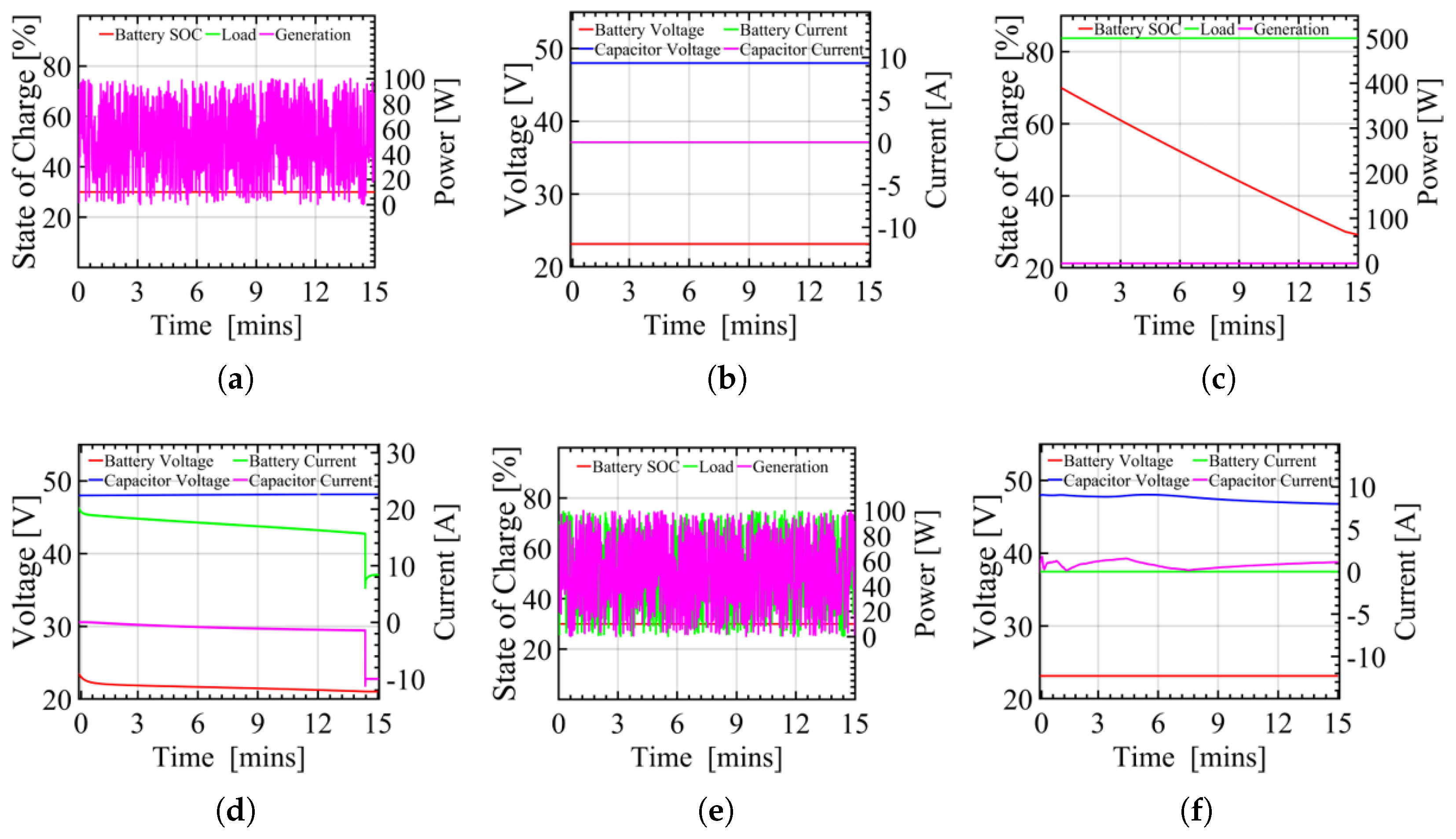
| Case | WEC Output (W) | Load Power Dammed (W) | SC F (V) | ESS V (Ahr) | SOC (%) |
|---|---|---|---|---|---|
| I | 0–100 | 0–100 | 10 (48) | 24 (10) | 30 |
| II | 0 | 500 | 10 (48) | 24 (10) | 70 |
| III | 0–100 | 0–100 | 10 (48) | 24 (10) | 30 |
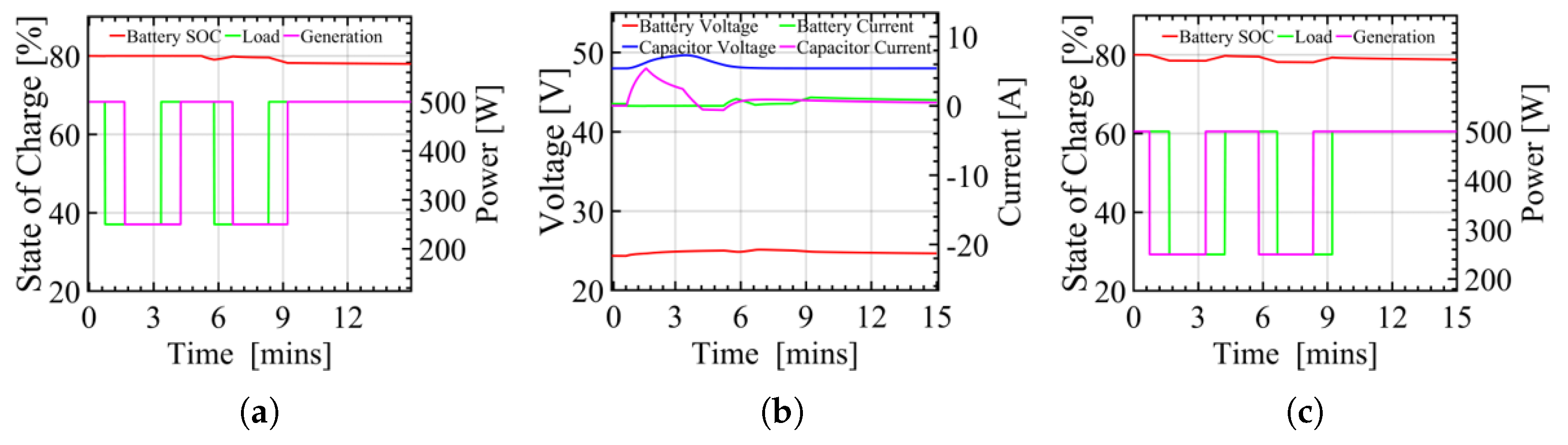
| IV | 250–500 | 250–500 | 10 (48) | 24 (10) | 80 |
| V | 250–500 | 500–250 | 10 (48) | 24 (10) | 80 |
| VI | 0–100 | 0–100 | 10 (48) | 24 (10) | 30 |
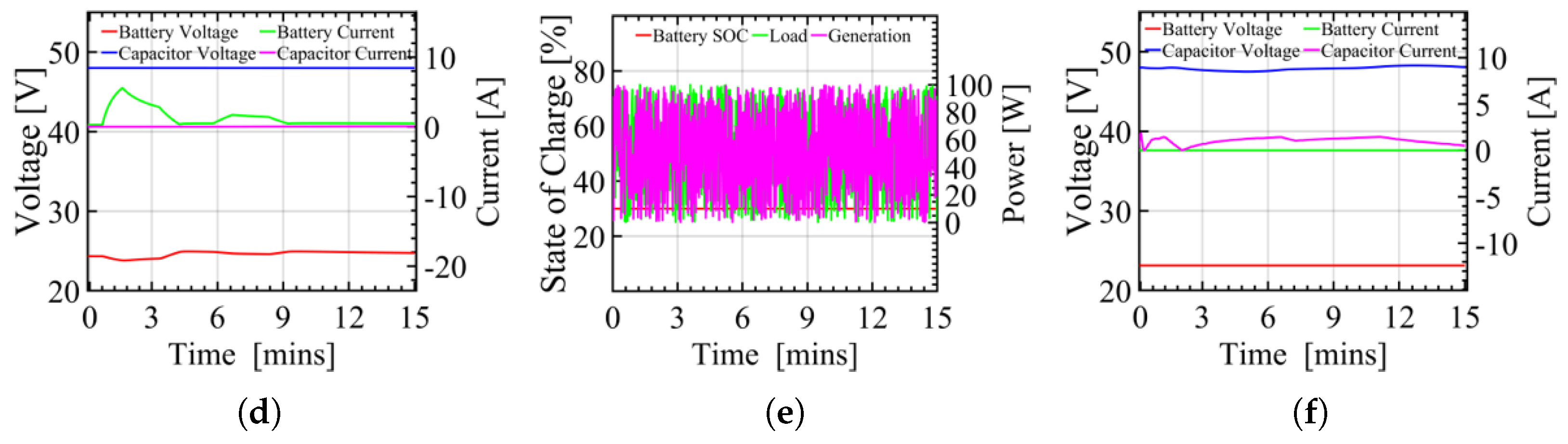
| VII | 500 | 250–500 | 10 (48) | 24 (10) | 30 |
| VIII | 250–500 | 500 | 10 (48) | 24 (10) | 77 |
| IX | 0–250 | 250 | 10 (48) | 24 (10) | 35 |
Disclaimer/Publisher’s Note: The statements, opinions and data contained in all publications are solely those of the individual author(s) and contributor(s) and not of MDPI and/or the editor(s). MDPI and/or the editor(s) disclaim responsibility for any injury to people or property resulting from any ideas, methods, instructions or products referred to in the content. |
© 2024 by the authors. Licensee MDPI, Basel, Switzerland. This article is an open access article distributed under the terms and conditions of the Creative Commons Attribution (CC BY) license (https://creativecommons.org/licenses/by/4.0/).
Share and Cite
Iqbal, S.; Mehran, K. Data-Driven Management Systems for Wave-Powered Renewable Energy Communities. Energies 2024, 17, 1197. https://doi.org/10.3390/en17051197
Iqbal S, Mehran K. Data-Driven Management Systems for Wave-Powered Renewable Energy Communities. Energies. 2024; 17(5):1197. https://doi.org/10.3390/en17051197
Chicago/Turabian StyleIqbal, Saqib, and Kamyar Mehran. 2024. "Data-Driven Management Systems for Wave-Powered Renewable Energy Communities" Energies 17, no. 5: 1197. https://doi.org/10.3390/en17051197
APA StyleIqbal, S., & Mehran, K. (2024). Data-Driven Management Systems for Wave-Powered Renewable Energy Communities. Energies, 17(5), 1197. https://doi.org/10.3390/en17051197