
Numerical Simulation of Vertical Well Depressurization with Different Deployments of Radial Laterals in Class 1-Type Hydrate Reservoir

 , ,
, ,
Abstract
1. Introduction
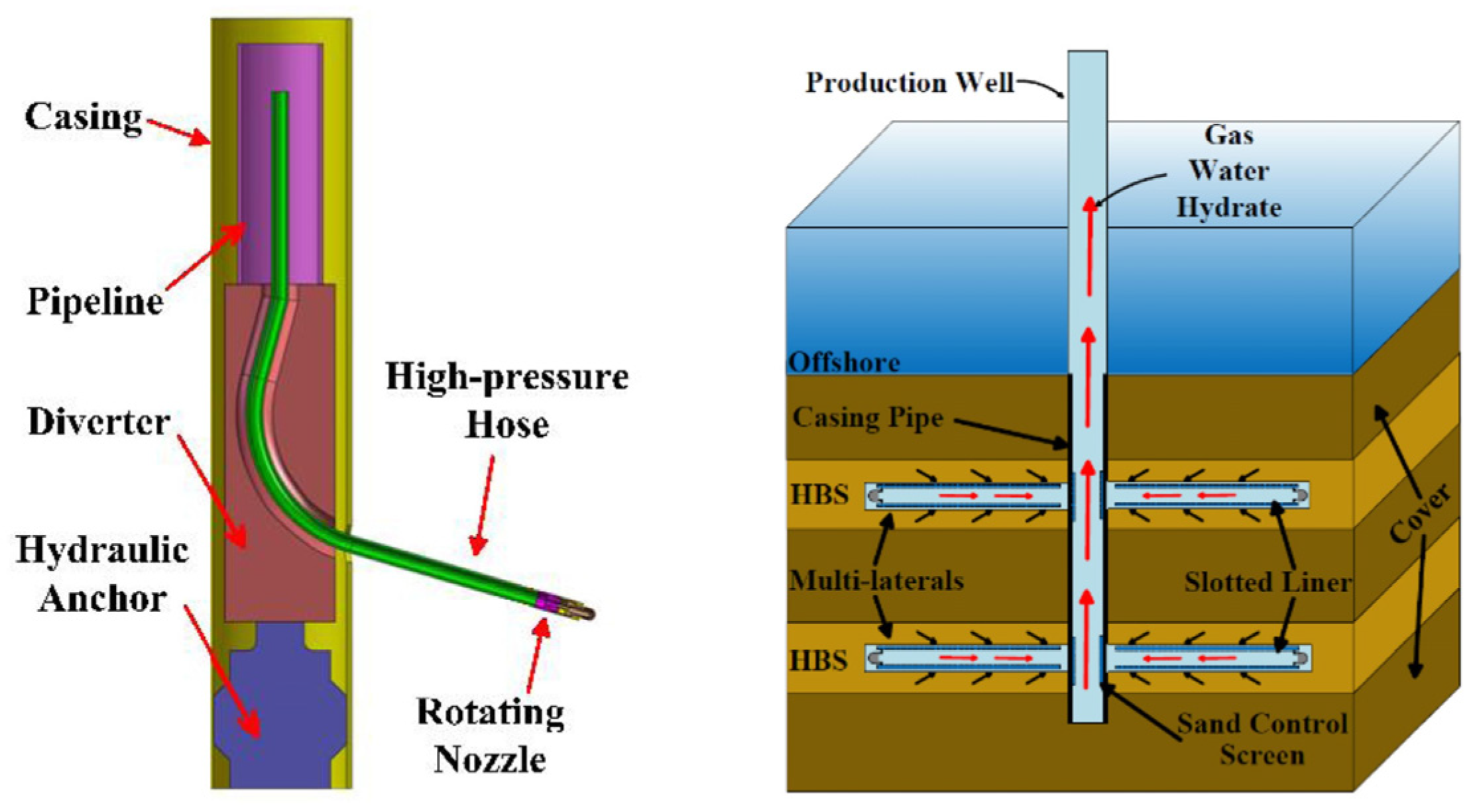
2. Radial Jet Drilling
3. Methodology
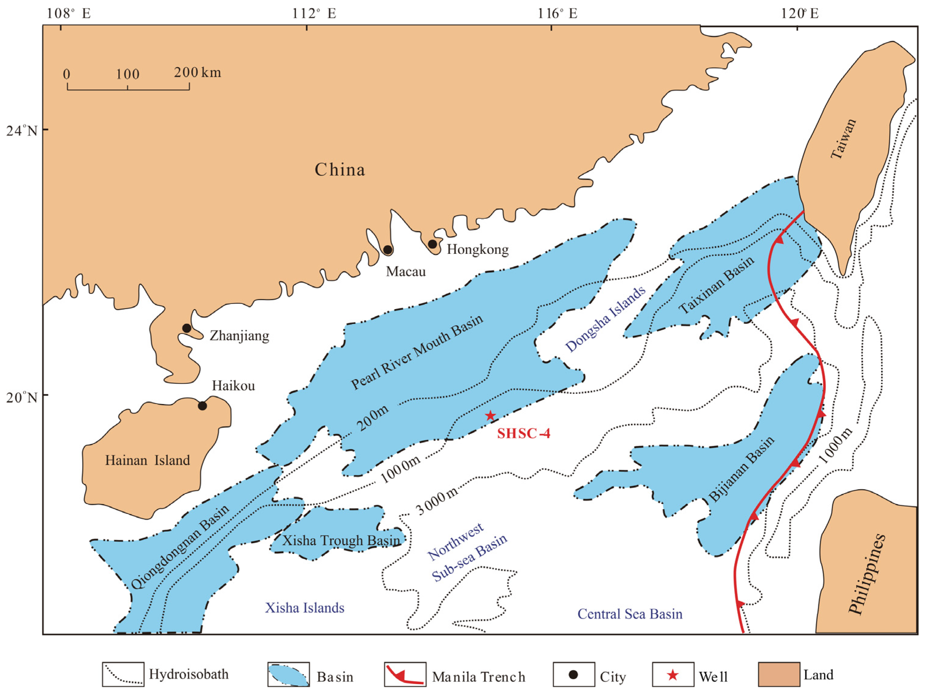
3.1. Geological Background
3.2. Simulation Code
- 1.
- Phases and components
- 2.
- Mass balance
- 3.
- Energy balance
- 4.
- Phase changes
- 5.
- Stress
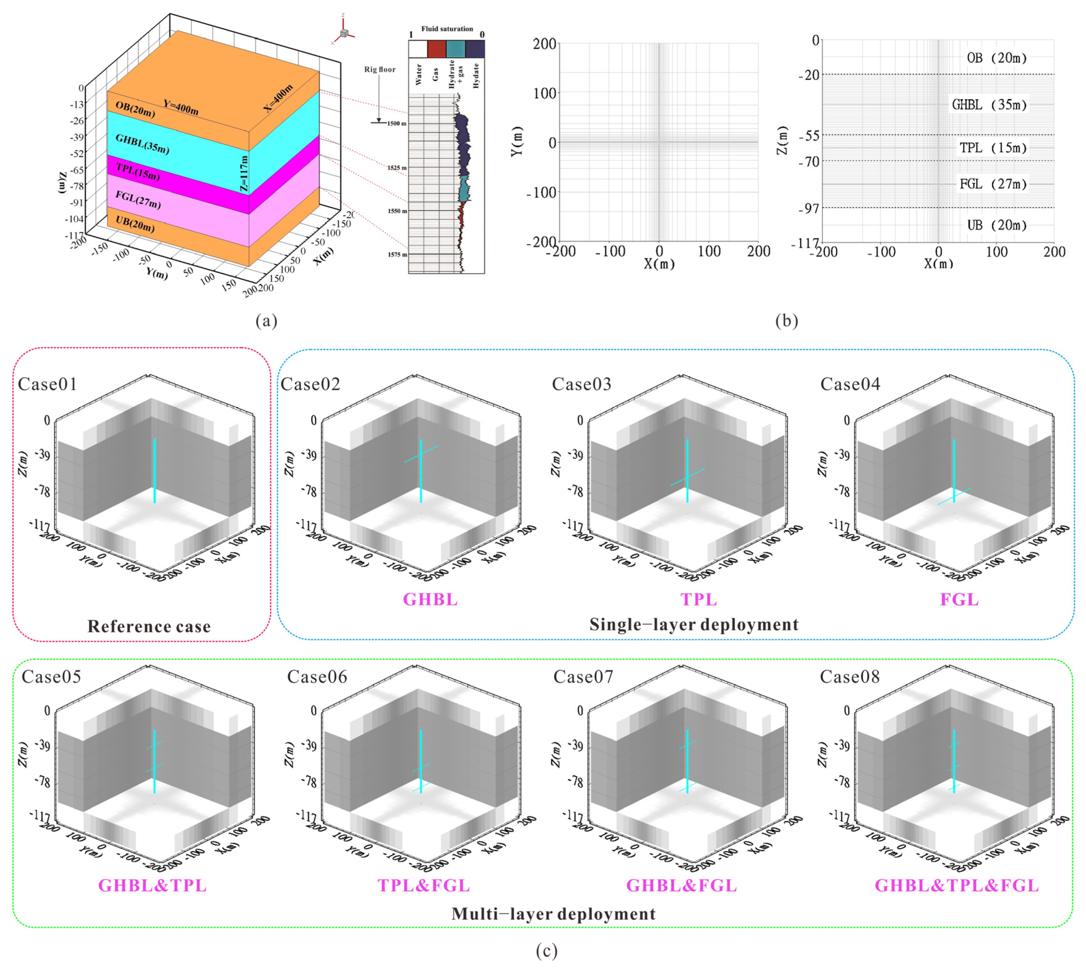
3.3. Model Construction and Case Design
3.4. Initial and Boundary Conditions
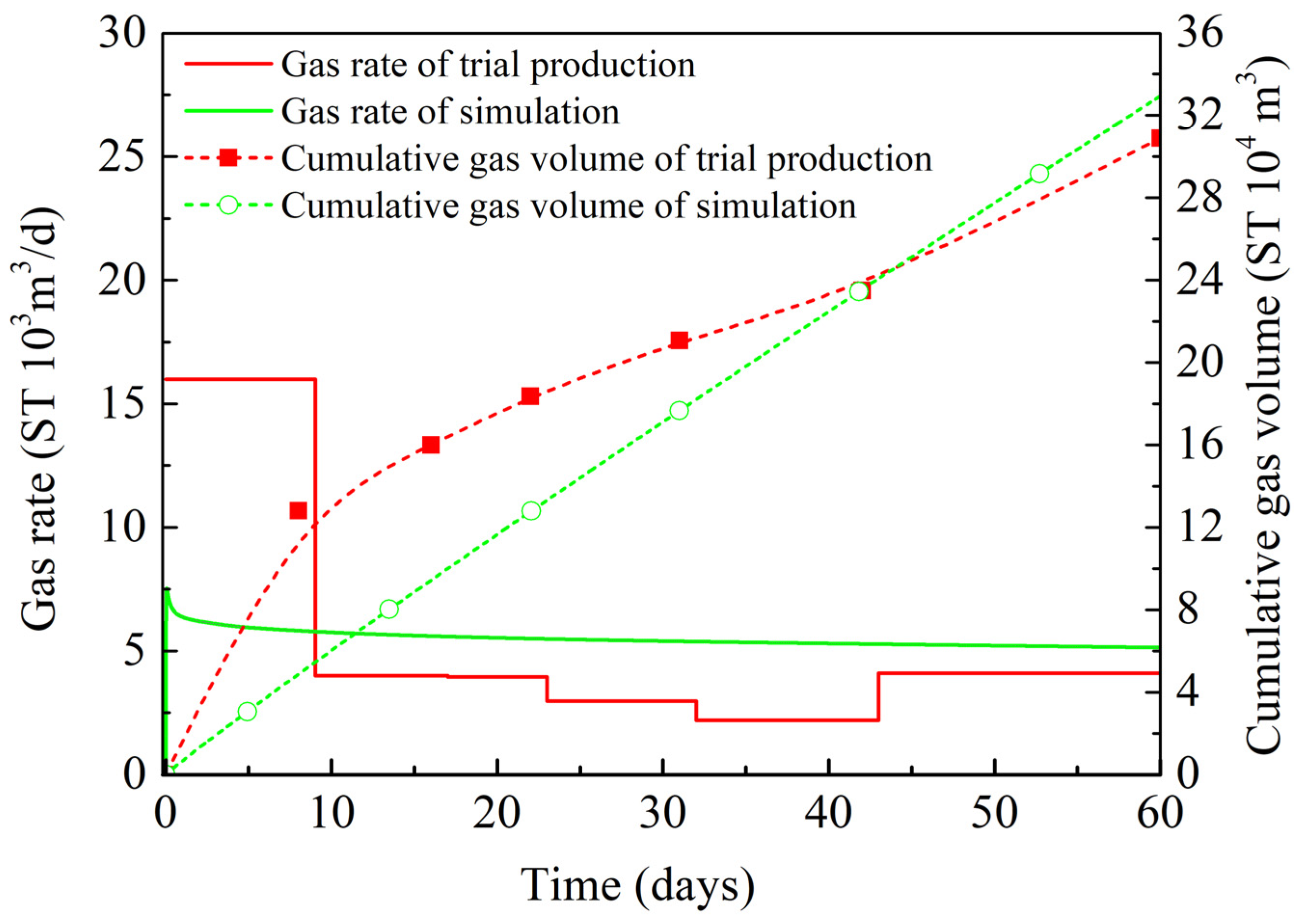
3.5. Model Validation
4. Results and Discussion
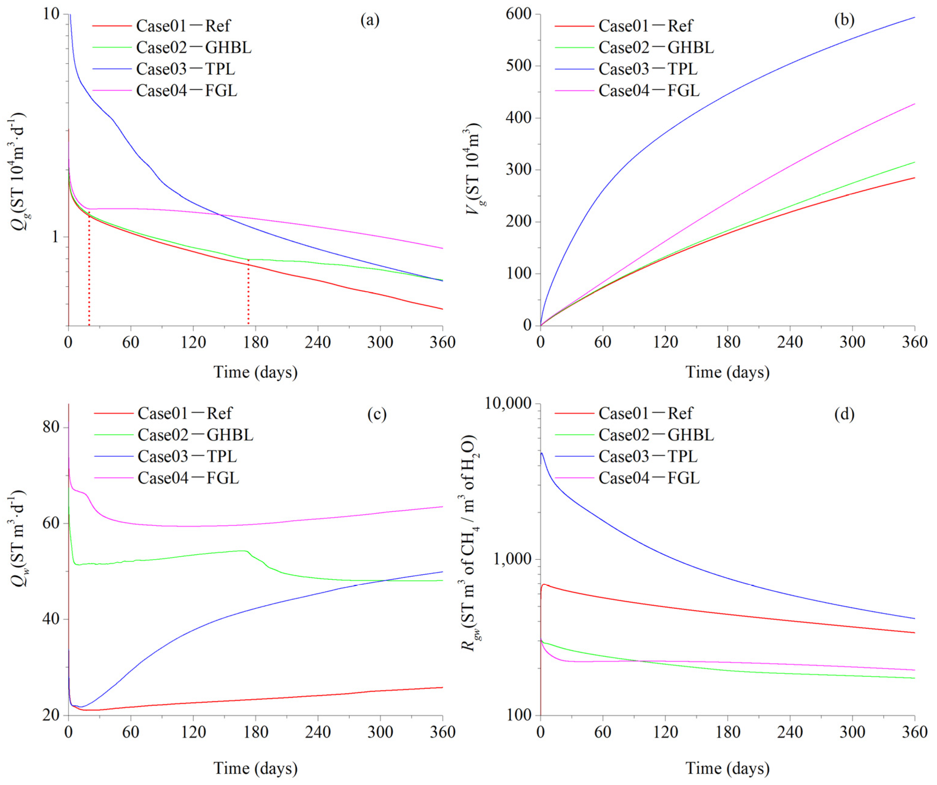
4.1. Single-Layer Deployment
4.1.1. Gas and Water Production
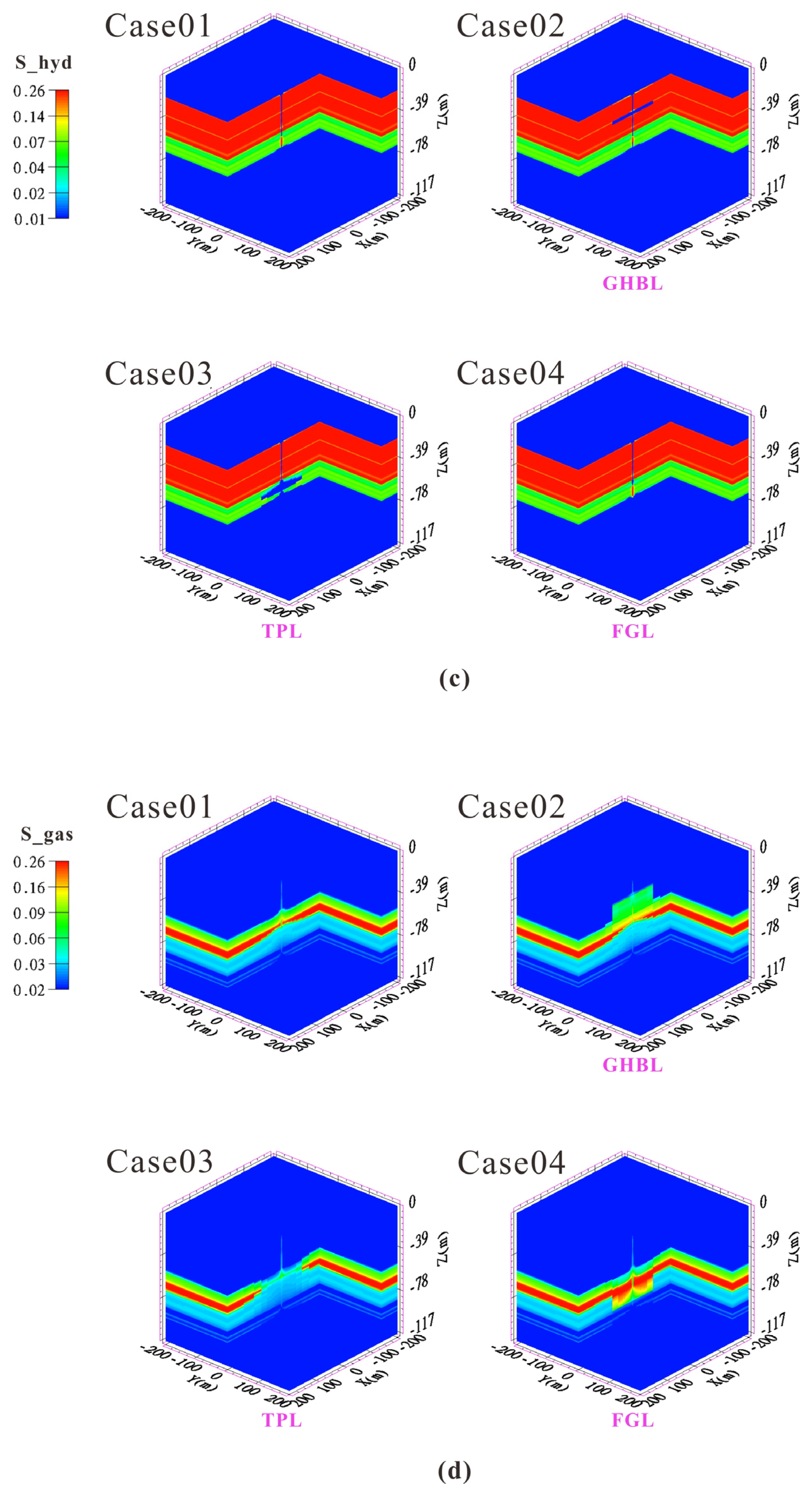
4.1.2. Spatial Distribution of Physical Properties
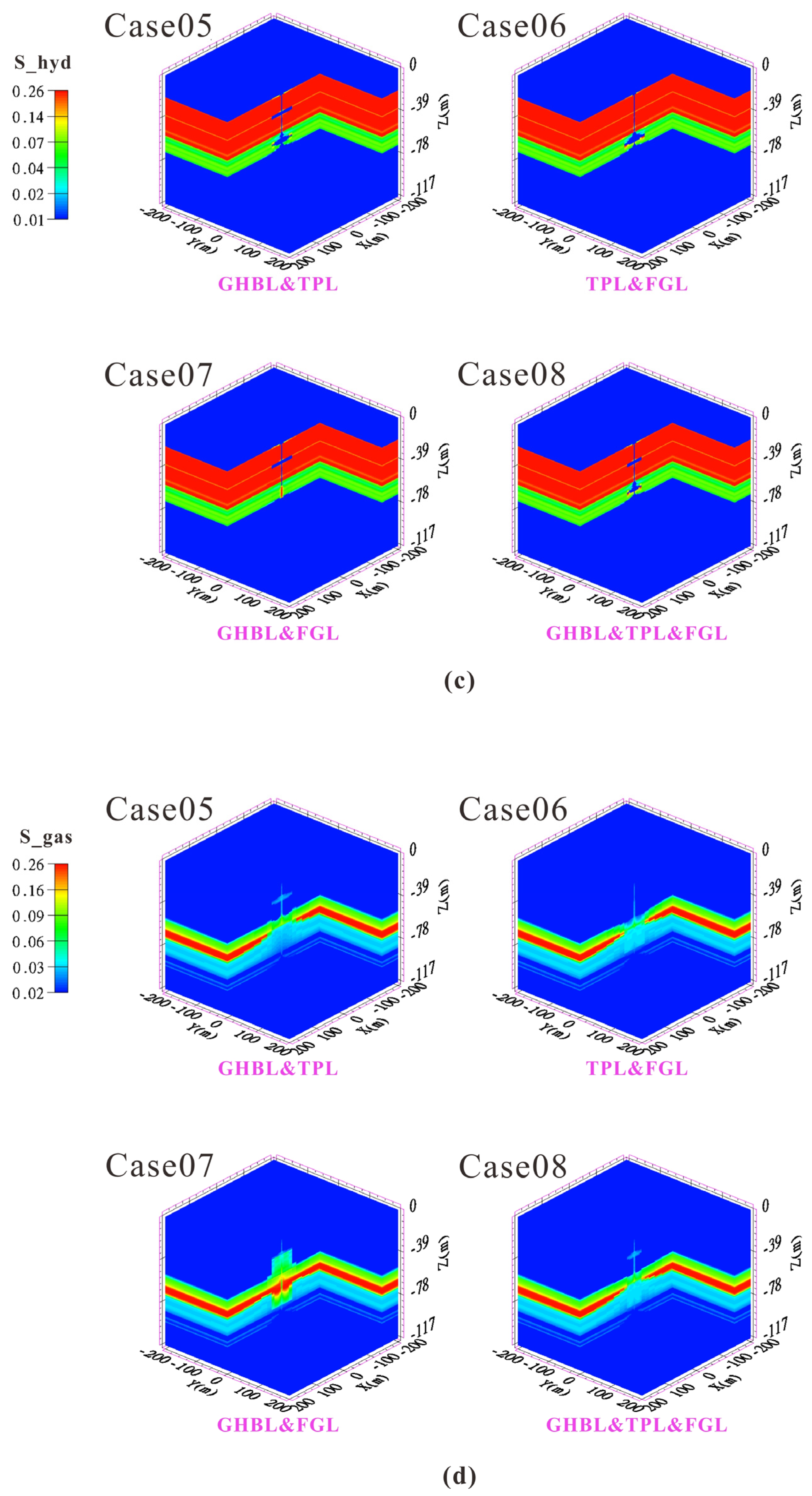
4.2. Multi-Layer Deployment
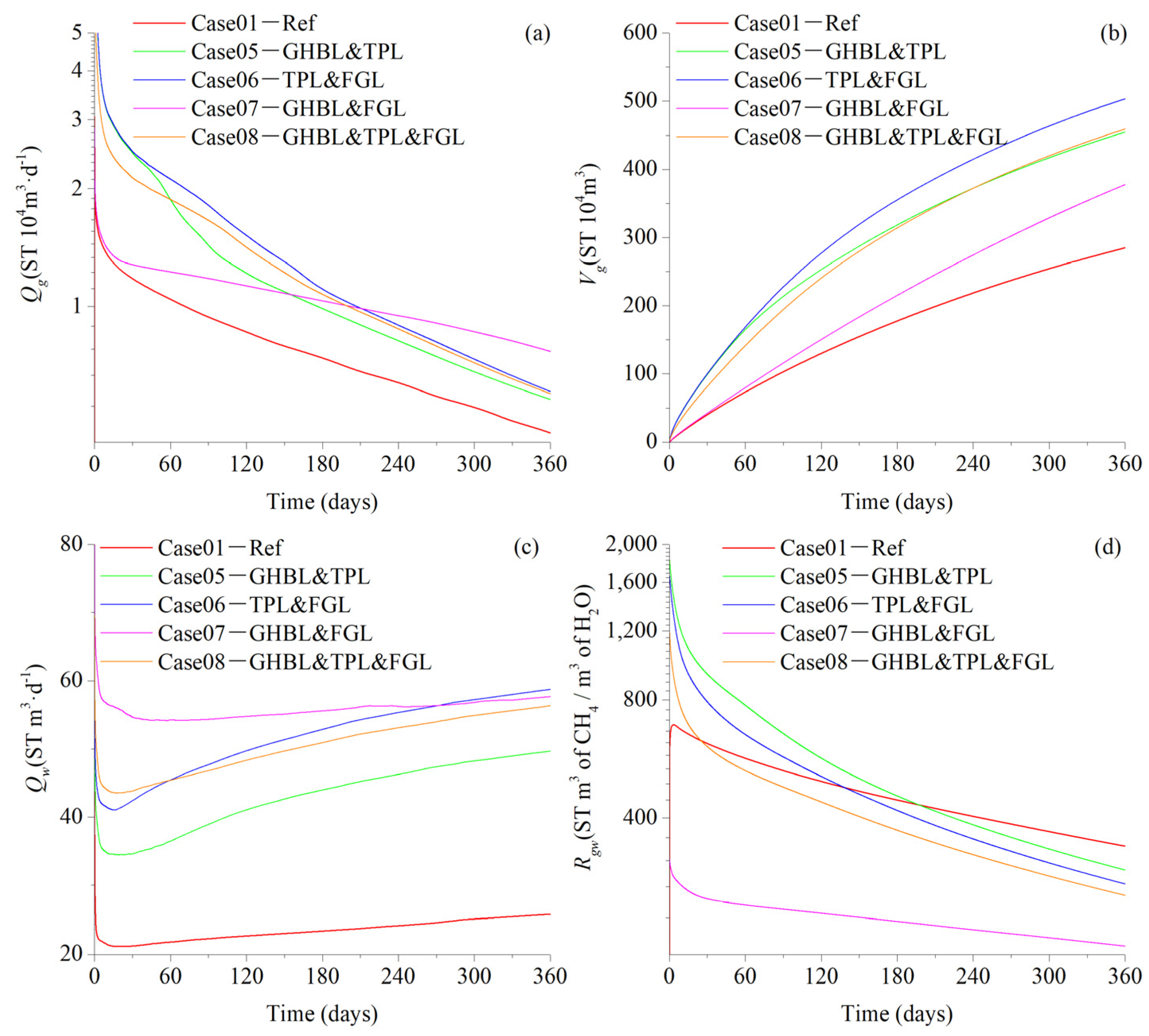
4.2.1. Gas and Water Production
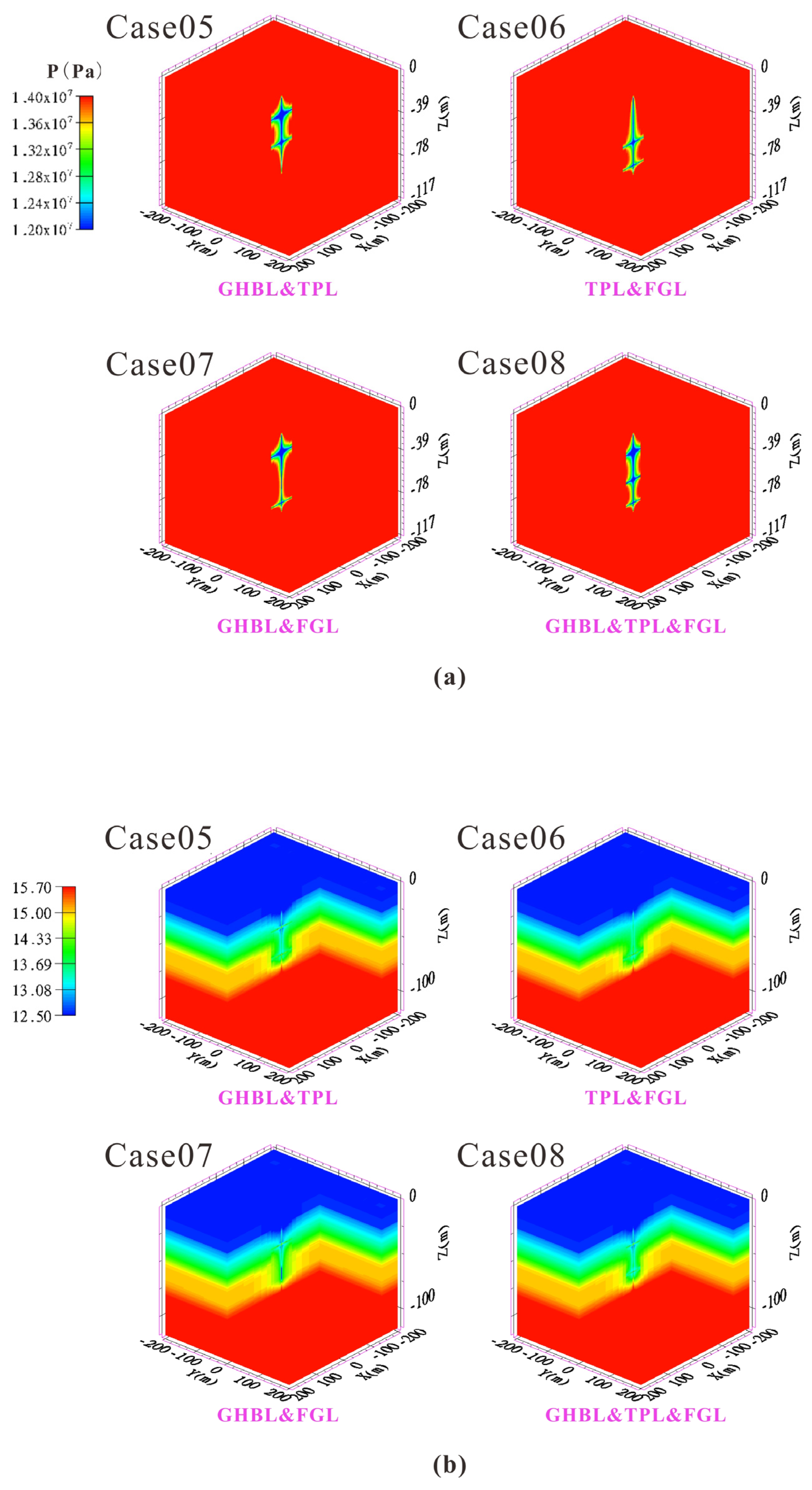
4.2.2. Spatial Distribution of Physical Properties
4.3. Comparisons of Production Performances
5. Conclusions
Author Contributions
Funding
Data Availability Statement
Conflicts of Interest
Nomenclature
| Symbols | Abbreviations | ||
| L | open hole completion length (m) | OB | overburden layer |
| n | quantity of lateral | UB | underburden layer |
| l | lateral length (m) | GHBL | gas hydrate-bearing layer |
| x, y, z | cartesian coordinates (m) | TPL | Three-phase layer |
| Qg | gas production rates at well (m3/d) | FGL | free gas layer |
| Qw | water production rates at well (m3/d) | NGH | natural gas hydrate |
| Vg | cumulative gas production at well (m3/d) | RJD | Radial jet drilling |
| Rgw | ratio of cumulative gas to cumulative gas (ST m3 of CH4/m3 of H2O) | ||
| mass accumulation of component κ, (kg/m3) | |||
| mass flux of component κ, kg/(m2·s) | |||
| sink/source of component κ, kg/(m3·s) | |||
| energy accumulation (J/m3) | |||
| energy flux, J/(m2·s) | |||
| sink/source of heat, J/(m3·s) | |||
| volume (m3) | |||
| surface area (m2) | |||
| t | times (s) | ||
| φ | porosity | ||
| Sβ | saturation of phase β | ||
| ρβ | density of phase β | ||
| mass fraction of component κ in phase β | |||
| k | permeability (m2) | ||
| krβ | relative permeability of phase β | ||
| viscosity of phase β, (Pa·s) | |||
| pressure of phase β, (Pa) | |||
| g | gravity acceleration (m/s2) | ||
| b | Klinkenberg factor (Pa) | ||
| medium tortuosity of phase β | |||
| molecular diffusion coefficient of component κ in phase β, (m2/s) | |||
| ρR | density of rock grain (kg/m3) | ||
| specific heat of rock grain, J/(kg·°C) | |||
| T | temperature (°C) | ||
| internal energy of phase β, (J/kg) | |||
| λ | average thermal conductivity, W/(m·K) | ||
| specific enthalpy of phase β, (J/kg) | |||
| mass diffusion of component κ in phase β, kg/(m2·s) | |||
| hydrate density, (kg/m3) | |||
| hydrate saturation | |||
| specific enthalpy of hydrate dissociation/formation, J/kg | |||
| mass change of hydrate component under kinetic dissociation, kg | |||
| hydration number | |||
| gradient operator | |||
| β | phase, β = A, G, H, I is aqueous, gas, hydrate and ice, respectively | ||
| κ | component, κ = w, m, i, h is water, methane, salt, and hydrate, respectively | ||
| T | phase equilibrium temperature (K) | ||
| e1 | regression parameter | ||
| e2 | regression parameter | ||
| available porosity for fluids | |||
| relative magnitude of | |||
| solid saturation | |||
| porosity adjustment factor | |||
| pore compressibility expansivity | |||
| pore thermal expansivity | |||
| Pcap | capillary pressure (Pa) | ||
| P0 | entry pressure of capillary pressure model (Pa) | ||
| S* | saturation for capillary pressure model | ||
| SmxA | maximum reference aqueous saturation of capillary | ||
| SirA | irreducible saturation of aqueous phase | ||
| SirG | irreducible saturation of gas phase | ||
| nA | permeability reduction exponent for aqueous phase | ||
| nG | permeability reduction exponent for gas phase | ||
| λ | parameter of capillary pressure model | ||
References
- Sloan, E.D. Fundamental principles and applications of natural gas hydrates. Nature 2003, 426, 353–359. [Google Scholar] [CrossRef]
- Boswell, R. Is gas hydrate energy within reach? Science 2009, 325, 957–958. [Google Scholar] [CrossRef]
- Chong, Z.R.; Yang, S.H.B.; Babu, P.; Linga, P.; Li, X.S. Review of natural gas hydrates as an energy resource: Prospects and challenges. Appl. Energy 2016, 162, 1633–1652. [Google Scholar] [CrossRef]
- Boswell, R.; Collett, T.S. Current perspectives on gas hydrate resources. Energy Environ. Sci. 2011, 4, 1206–1215. [Google Scholar] [CrossRef]
- Yamamoto, K.; Terao, Y.; Fujii, T.; Ikawa, T.; Seki, M.; Matsuzawa, M.; Kanno, T. Operational Overview of the First Offshore Production Test of Methane Hydrates in the Eastern Nankai Trough. In Proceedings of the Offshore Technology Conference, Houston, TX, USA, 7 May 2014. [Google Scholar]
- Yamamoto, K.; Wang, X.X.; Tamaki, M.; Suzuki, K. The second offshore production of methane hydrate in the Nankai Trough and gas production behavior from a heterogeneous methane hydrate reservoir. RSC Adv. 2019, 9, 25987–26013. [Google Scholar] [CrossRef]
- Li, J.F.; Ye, J.L.; Qin, X.W.; Qiu, H.J.; Wu, N.Y.; Lu, H.L.; Xie, W.W.; Lu, J.A.; Peng, F.; Xu, Z.Q.; et al. The first offshore natural gas hydrate production test in South China Sea. China Geol. 2018, 1, 5–16. [Google Scholar] [CrossRef]
- Ye, J.L.; Qin, X.W.; Xie, W.W.; Lu, H.L.; Ma, B.J.; Qiu, H.J.; Liang, J.Q.; Lu, J.A.; Kuang, Z.G.; Lu, C.; et al. The second natural gas hydrate production test in the South China Sea. China Geol. 2020, 3, 197–209. [Google Scholar] [CrossRef]
- Cinelli, S.D.; Kamel, A.H. Novel technique to drill horizontal laterals revitalizes aging field. In Proceedings of the SPE/IADC Drilling Conference and Exhibition, Amsterdam, The Netherlands, 5–7 March 2013. [Google Scholar]
- Mahmood, M.N.; Guo, B. Productivity comparison of radial lateral wells and horizontal snake wells applied to marine gas hydrate reservoir development. Petroleum 2021, 7, 407–413. [Google Scholar] [CrossRef]
- Kamel, A.H. Radial Jet Drilling: A Technical Review. In Proceedings of the SPE Middle East Oil & Gas Show and Conference, Manama, Kingdom of Bahrain, 8 March 2017. [Google Scholar]
- Kamel, A.H. A technical review of radial jet drilling. J. Pet. Gas Eng. 2017, 8, 79–89. [Google Scholar]
- Huang, Z.; Huang, Z.W. Review of Radial Jet Drilling and the key issues to be applied in new geo-energy exploitation. Energy Procedia 2019, 158, 5969–5974. [Google Scholar] [CrossRef]
- Li, G.S.; Tian, S.C.; Zhang, Y.Q. Research progress on key technologies of natural gas hydrate exploitation by cavitation jet drilling of radial wells. Pet. Sci. Bulletin 2020, 5, 349–365. [Google Scholar]
- Zhang, P.P.; Tian, S.C.; Zhang, Y.Q.; Li, G.S.; Zhang, W.H.; Khan, W.A.; Ma, L.Y. Numerical simulation of gas recovery from natural gas hydrate using multi-branch wells: A three-dimensional model. Energy 2020, 220, 119549. [Google Scholar] [CrossRef]
- Zhang, P.P.; Tian, S.C.; Zhang, Y.Q.; Li, G.S.; Wu, X.Y.; Wang, Y.H. Production simulation of natural gas hydrate using radial well depressurization. Pet. Sci. Bull. 2021, 3, 417–428. [Google Scholar]
- Zhang, Y.Q.; Wu, X.Y.; Hu, X.; Zhang, B.; Lu, J.S.; Zhang, P.P.; Li, G.S.; Tian, S.C.; Li, X.M. Visualization and investigation of the erosion process for natural gas hydrate using water jet through experiments and simulation. Energy Rep. 2022, 8, 202–216. [Google Scholar] [CrossRef]
- Zhang, P.P.; Zhang, Y.Q.; Wang, W.; Wang, T.Y.; Tian, S.C. Experimental study on natural gas hydrate extraction with radial well depressurization. Pet. Sci. Bull. 2022, 03, 382–393. [Google Scholar]
- Hui, C.Y.; Zhang, Y.Q.; Zhang, P.P.; Wu, X.Y.; Huang, H.C.; Li, G.S. A study of natural gas hydrate reservoir stimulation by combining radial well fracturing and depressurization. In Proceedings of the ARMA US Rock Mechanics/Geomechanics Symposium, Santa Fe, NM, USA, 26–29 June 2022. [Google Scholar]
- Hui, C.Y.; Zhang, Y.Q.; Zhang, P.P.; Wu, X.Y.; Li, G.S.; Huang, H.C. Numerical simulation of natural gas hydrate productivity based on radial well fracturing combined with the depressurization method. Nat. Gas Ind. 2022, 42, 152–164. [Google Scholar]
- Li, G.S.; Huang, Z.W.; Li, J.B. Study of radial jet drilling key issues. Pet. Drill. Tech. 2017, 45, 1–9. [Google Scholar]
- Yang, D.; Gao, Q.Y.; Zhu, Y.J.; Zhang, X.Q.; Zheng, B.D.; Wu, X.C. Research and application of radial hydraulic jet drilling technology in oil and gas wells. Well Test. 2017, 26, 67–69. [Google Scholar]
- Song, X.Z.; Shi, Y.; Li, G.S.; Yang, R.Y.; Wang, G.S.; Zheng, R.; Li, J.C.; Lyu, Z.H. Numerical simulation of heat extraction performance in enhanced geothermal system with multilateral wells. Appl. Energy 2018, 218, 325–337. [Google Scholar] [CrossRef]
- Zhang, W.; Liang, J.Q.; Lu, J.A.; Wei, J.G.; Su, P.B.; Fang, Y.X.; Guo, Y.Q.; Yang, S.X.; Zang, G.X. Accumulation features and mechanisms of high saturation natural gas hydrate in shenhu area, northern south china sea. Pet. Explor. Dev. 2017, 44, 708–719. [Google Scholar] [CrossRef]
- Moridis, G.J.; Kowalsky, M.B.; Pruess, K. TOUGH+ Hydrate V1.0 User’s Manual; Report LBNL-0149E; Lawrence Berkeley National Laboratory: Berkeley, CA, USA, 2008. [Google Scholar]
- Su, Z.; Moridis, G.J.; Zhang, K.N.; Wu, N.Y. A huff-and-puff production of gas hydrate deposits in Shenhu area of South China Sea through a vertical well. J. Pet. Sci. Eng. 2012, 86–87, 54–61. [Google Scholar] [CrossRef]
- Yin, Z.Y.; Moridis, G.J.; Chong, Z.R.; Linga, P. Effectiveness of multi-stage cooling processes in improving the CH4-hydrate saturation uniformity in sandy laboratory samples. Appl. Energy 2019, 250, 729–747. [Google Scholar] [CrossRef]
- Zhang, K.N.; Moridis, G.J.; Wu, Y.S.; Pruess, K. A domain decompositionapproach for large-scale simulations of flow processes in hydrate-bearing geologic media. In Proceedings of the 6th International Conference on Gas Hydrates, Vancouver, BC, Canada, 6–10 July 2008; ICGH: Vancouver, BC, Canada, 2009. [Google Scholar]
- Kowalsky, M.B.; Moridis, G.J. Comparison of kinetic and equilibrium reaction models in simulating gas hydrate behavior in porous media. Energy Convers. Manag. 2007, 48, 1850–1863. [Google Scholar] [CrossRef]
- Li, G.; Li, X.S.; Zhang, K.N.; Li, B.; Zhang, Y. Effects of Impermeable Boundaries on Gas Production from Hydrate Accumulations in the Shenhu Area of the South China Sea. Energies 2013, 6, 4078–4096. [Google Scholar] [CrossRef]
- Yu, T.; Guan, G.Q.; Wang, D.Y.; Song, Y.C.; Abudula, A. Numerical investigation on the long-term gas production behavior at the 2017 Shenhu methane hydrate production-site. Appl. Energy 2021, 285, 116466. [Google Scholar] [CrossRef]
- Sun, J.X.; Zhang, L.; Ning, F.L.; Lei, H.W.; Liu, T.L.; Hu, G.W.; Lu, H.L.; Lu, J.A.; Liu, C.L.; Jiang, G.S.; et al. Production potential and stability of hydrate-bearing sediments at the site GMGS3-W19 in the South China Sea: A preliminary feasibility study. Mar. Pet. Geol. 2017, 86, 447–473. [Google Scholar] [CrossRef]
- Yuan, Y.L.; Xu, T.F.; Xin, X.X.; Xia, Y.L. Multiphase Flow Behavior of Layered Methane Hydrate Reservoir Induced by Gas Production. Geofluids 2017, 2017, 1–15. [Google Scholar] [CrossRef]
- Sun, J.X.; Ning, F.L.; Li, S.; Zhang, K.; Liu, T.L.; Zhang, L.; Jiang, G.S.; Wu, N.Y. Numerical simulation of gas production from hydrate-bearing sediments in the Shenhu area by depressurising: The effect of burden permeability. J. Unconv. Oil Gas Resour. 2015, 12, 23–33. [Google Scholar] [CrossRef]
- Feng, Y.C.; Chen, L.; Suzuki, A.; Kogawa, T.; Okajima, J.; Komiya, A.; Maruyama, S. Enhancement of gas production from methane hydrate reservoirs by the combination of hydraulic fracturing and depressurization method. Energy Convers. Manag. 2019, 184, 194–204. [Google Scholar] [CrossRef]
- Moridis, G.J.; Reagan, M.T.; Kim, S.J.; Seol, Y.; Zhang, K. Evaluation of the Gas Production Potential of Marine Hydrate Deposits in the Ulleung Basin of the Korean East Sea. SPE J. 2007, 14, 759–781. [Google Scholar] [CrossRef]
- Sun, Y.H.; Ma, X.L.; Guo, W.; Jia, R.; Li, B. Numerical simulation of the short- and long-term production behavior of the first offshore gas hydrate production test in the South China Sea. J. Pet. Sci. Eng. 2019, 181, 106196. [Google Scholar] [CrossRef]
- Ma, X.L.; Sun, Y.H.; Liu, B.C.; Guo, W.; Jia, R.; Li, B.; Li, S.L. Numerical study of depressurization and hot water injection for gas hydrate production in China’s first offshore test site. J. Pet. Sci. Eng. 2020, 83, 103530. [Google Scholar] [CrossRef]
- Cao, X.X.; Sun, J.X.; Qin, F.F.; Ning, F.L.; Mao, P.X.; Gu, Y.H.; Li, Y.L.; Zhang, H.; Yu, Y.J.; Wu, N.Y. Numerical analysis on gas production performance by using a multilateral well system at the first offshore hydrate production test site in the Shenhu area. Energy 2023, 270, 126690. [Google Scholar] [CrossRef]
- Qin, X.W.; Liang, Q.Y.; Ye, J.L.; Yang, L.; Qiu, H.J.; Xie, W.W.; Liang, J.Q.; Lu, J.A.; Lu, C.; Lu, H.L.; et al. The response of temperature and pressure of hydrate reservoirs in the first gas hydrate production test in South China Sea. Appl. Energy 2020, 278, 115649. [Google Scholar] [CrossRef]


| Groups | Case | Main Parameters of Radial Laterals | |||
|---|---|---|---|---|---|
| n | l (m) | L (m) | Deployment Location | ||
| Single vertical well | Case 01 | - | - | - | - |
| Single-layer deployment | Case 02 | 2 | 75 | 150 | GHBL |
| Case 03 | 2 | 75 | 150 | TPL | |
| Case 04 | 2 | 75 | 150 | FGL | |
| Multi-layer deployment | Case 05 | 4 | 37.5 | 150 | GHBL & TPL |
| Case 06 | 4 | 37.5 | 150 | TPL & FGL | |
| Case 07 | 4 | 37.5 | 150 | GHBL & FGL | |
| Case 08 | 6 | 25 | 150 | GHBL & TPL & FGL | |
| Parameter | Value & Unit |
|---|---|
| OB and UB thickness | 20 m |
| GHBL thickness | 35 m |
| TPL thickness | 15 m |
| FGL thickness | 27 m |
| OB and UB permeability | 2.0 mD |
| GHBL permeability | 2.9 mD |
| TPL permeability | 1.5 mD |
| FGL permeability | 7.4 mD |
| Vertical wellbore length | 70 m, in accordance with the model’s −21 m to −91 m |
| Vertical wellbore radius | 0.1 m |
| Radial laterals radius [10] | 50 mm |
| Salinity | 3.5% |
| GHBL and TPL hydrate saturation | Reference from logging curve (Figure 3a) |
| FGL gas saturation | Reference from logging curve (Figure 3a) |
| OB and UB porosity | 0.30 |
| GHBL porosity | 0.35 |
| TPL porosity | 0.33 |
| FGL porosity | 0.32 |
| Grain density | 2600 kg/m3 |
| Geothermal gradient | 43.653 °C/km |
| Grain specific heat | 1000 J·kg−1·K−1 |
| Gas composition | 100% CH4 |
| Dry thermal conductivity | 1.0 W·m−1·K−1 |
| Wet thermal conductivity | 3.1 W·m−1·K−1 |
| Capillary pressure model [37,38,39] | , |
| SmxA | 1 |
| λ | 0.45 |
| P0 | 104 Pa |
| Relative permeability model [37,38,39] | KrA = [(SA − SirA)/(1 − SirA)]nA, KrG = [(SG − SirG)/(1 − SirA)]nG |
| nA | 3.5 |
| nG | 2.5 |
| SirG | 0.03 |
| SirA | 0.30 |
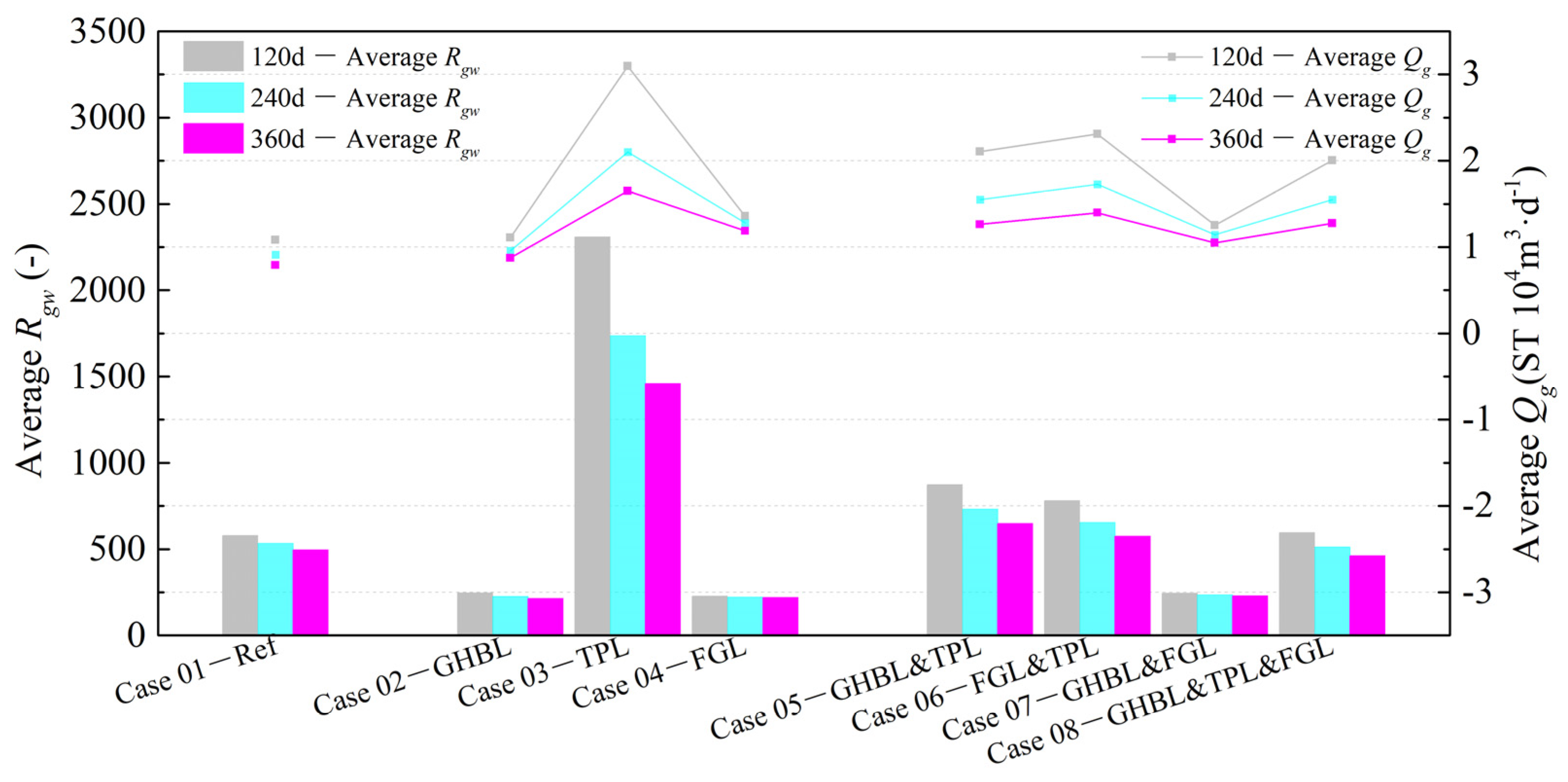
| Case | Deployment Location | Wellbore Contact Area (m2) | Average Qg (104 m3/d) | Vg (104 m3) | Compared to the Reference Case |
|---|---|---|---|---|---|
| Case 03 | GHBL | 91.10 | 1.65 | 594.10 | 208.53% |
| Case 04 | TPL | 91.10 | 1.19 | 427.50 | 150.05% |
| Case 02 | FGL | 91.10 | 0.87 | 314.80 | 110.49% |
| Case 01 (reference case) | - | 43.98 | 0.79 | 284.90 | 100.00% |
| Case | Deployment Location | Wellbore Contact Area (m2) | Average Qg (104 m3/d) | Vg (104 m3) | Compared to the Reference Case |
|---|---|---|---|---|---|
| Case 06 | TPL & FGL | 91.10 | 1.40 | 503.30 | 176.66% |
| Case 08 | GHBL & TPL & FGL | 91.10 | 1.28 | 459.00 | 161.11% |
| Case 05 | GHBL & TPL | 91.10 | 1.26 | 454.50 | 159.53% |
| Case 07 | GHBL & FGL | 91.10 | 1.05 | 377.60 | 132.54% |
| Case 01 (reference case) | - | 43.98 | 0.79 | 284.90 | 100.00% |
Disclaimer/Publisher’s Note: The statements, opinions and data contained in all publications are solely those of the individual author(s) and contributor(s) and not of MDPI and/or the editor(s). MDPI and/or the editor(s) disclaim responsibility for any injury to people or property resulting from any ideas, methods, instructions or products referred to in the content. |
© 2024 by the authors. Licensee MDPI, Basel, Switzerland. This article is an open access article distributed under the terms and conditions of the Creative Commons Attribution (CC BY) license (https://creativecommons.org/licenses/by/4.0/).
Share and Cite
Wan, T.; Yu, M.; Lu, H.; Chen, Z.; Li, Z.; Tian, L.; Li, K.; Huang, N.; Wang, J. Numerical Simulation of Vertical Well Depressurization with Different Deployments of Radial Laterals in Class 1-Type Hydrate Reservoir. Energies 2024, 17, 1139. https://doi.org/10.3390/en17051139
Wan T, Yu M, Lu H, Chen Z, Li Z, Tian L, Li K, Huang N, Wang J. Numerical Simulation of Vertical Well Depressurization with Different Deployments of Radial Laterals in Class 1-Type Hydrate Reservoir. Energies. 2024; 17(5):1139. https://doi.org/10.3390/en17051139
Chicago/Turabian StyleWan, Tinghui, Miao Yu, Hongfeng Lu, Zongheng Chen, Zhanzhao Li, Lieyu Tian, Keliang Li, Ning Huang, and Jingli Wang. 2024. "Numerical Simulation of Vertical Well Depressurization with Different Deployments of Radial Laterals in Class 1-Type Hydrate Reservoir" Energies 17, no. 5: 1139. https://doi.org/10.3390/en17051139
APA StyleWan, T., Yu, M., Lu, H., Chen, Z., Li, Z., Tian, L., Li, K., Huang, N., & Wang, J. (2024). Numerical Simulation of Vertical Well Depressurization with Different Deployments of Radial Laterals in Class 1-Type Hydrate Reservoir. Energies, 17(5), 1139. https://doi.org/10.3390/en17051139